Dynamics and spectral theory of quasi-periodic Schrödinger-type operators

1. Introduction

Quasi-periodic Schrödinger-type operators naturally arise in solid state physics, describing the influence of an external magnetic field on the electrons of a crystal. In the late 1970s, numerical studies for the most prominent model, the almost Mathieu operator (AMO), produced the first example of a fractal in physics known as “Hofstadter’s butterfly” [84], marking the starting point for the ongoing strong interest in such operators in both mathematics (several of B. Simon’s problems [154, 156]) and physics (e.g. Graphene, quantum Hall effect).

Whereas research in the first three decades was focused mainly on unraveling the unusual properties of the AMO and operators with similar structure of potential, in recent years a combination of techniques from dynamical systems with those from spectral theory has allowed for a more “global,” model-independent point of view. Intriguing phenomena first encountered for the AMO, notably the appearance of criticality corresponding to purely singular continuous (sc) spectrum for a measure theoretically typical realization of the phase, could be tested for prevalence in general models.

The intention of this article is to survey the theory of quasi-periodic Schrödinger-type operators attaining this “global” view-point with an emphasis on dynamical aspects of the spectral theory of such operators. For a more “traditional” review centered about the AMO we refer to e.g. [89].

2. Set up

Fix $d,\nu\in\mathbb{N}$. A quasi-periodic $\nu$-frequency, matrix valued Schrödinger-type operator (on the line) is a family of self-adjoint, bounded operators on $\mathit{l}^{2}(\mathbb{Z},\mathbb{C}^{d})$ indexed by points $\theta\in\mathbb{T}^{\nu}:=\mathbb{R}^{\nu}/\mathbb{Z}^{\nu}$ of the form

(2.1) $$[H_{\alpha,\theta}\psi]_{n}:=C(T_{\alpha}^{n-1}\theta)^{*}\psi_{n-1}+C(T_{\alpha}^{n}\theta)\psi_{n+1}+V(T_{\alpha}^{n}\theta)\psi_{n}~{}\mbox{.}$$

Here, for every realization of $\theta$, $H_{\theta}$ is generated by evaluating two matrix-valued sampling functions $C,V\in\mathcal{C}(\mathbb{T}^{\nu},M_{d}(\mathbb{C}))$, $V=V^{*}$, along the rotational trajectory induced by $(T_{\alpha}\theta)_{j}=\theta_{j}+\alpha_{j}$, $1\leq j\leq\nu$, where $\alpha\in\mathbb{T}^{\nu}$ is fixed with incommensurate components. $\theta$ is commonly called the phase, whereas $\alpha$ is referred to as the frequency.

We emphasize that $C(\theta)$ in (2.1) is not assumed to be invertible, in fact we call (2.1) singular if $\det C(\theta)=0$ for some $\theta\in\mathbb{T}^{\nu}$, and non-singular otherwise. For reasons of ergodicity we do however require that

(2.2) $$\log|\det C(.)|\in L^{1}(\mathbb{T}^{\nu})~{}\mbox{. }$$

Here, $\mathbb{T}^{\nu}$ is understood to be equipped with its Haar probability measure subsequently denoted by $\mathrm{d}^{\nu}\theta$ (or $|.|$ as a set function).

Presently, most results are known for $d=\nu=1$, which will also be the main focus of this article. The most widely studied special case arises when $d=1$ and $C\equiv 1$,

(2.3) $$[H_{\alpha,\theta}\psi]_{n}=\psi_{n-1}+\psi_{n+1}+V(T_{\alpha}^{n}\theta)\psi_{n}~{}\mbox{, }\psi\in\mathit{l}^{2}(\mathbb{Z},\mathbb{C})~{}\mbox{,}$$

which is commonly known as quasi-periodic Schrödinger operator. Probably because the most prominent quasi-periodic operator, the AMO where $V(\theta)=2\lambda\cos(2\pi\theta)$, $\lambda>0$, falls into this class, the majority of articles in the literature have focused on the special case (2.3).

From a physics point of view, however, the situation when $C\not\equiv 1$ or even has zeros is absolutely natural and cannot be excluded (cf. Sec. 2.1). To explicitly distinguish (2.3) from the general case (2.1), we shall from here on refer to the latter as (matrix-valued) Jacobi operator.

One of the contributions we hope to make with this review article, is to present a consistent picture for the general Jacobi case. Therefore, whenever the proof of a statement, originally in the literature for Schrödinger operators, has an obvious extension to the Jacobi case, we will give its Jacobi formulation. In some situations however, in particular when dealing with singular Jacobi operators, such extensions are not immediate and not in the literature, in which case we will state the theorems in their presently available Schrödinger form. In theses cases the authors hope to spark the interest in the reader to work on appropriate theorems applying to (singular) Jacobi operators.

Finally, we mention that at times we will contrast results for Schrödinger operators on $\mathbb{Z}$ with their analogue on higher dimensional lattices, $\mathbb{Z}^{N}$ for $N>1$, where the first two terms in (2.3) are correspondingly replaced by the $N$-dimensional discrete Laplacian. As the latter however do not lend themselves to the dynamical description central to this article, we will not describe the methods for their study here. An excellent reference for the Green’s function methods suitable for quasi-periodic operators on higher dimensional lattices is e.g. [36].

2.1. Origin in physics

In physics, quasi-periodic Jacobi operators arise as effective Hamiltonians in a tight-binding description of a crystal subject to a weak external magnetic field. In particular, the case $d=\nu=1$ describes the effects for a two dimensional crystalline layer with $\alpha\in\mathbb{T}$ corresponding to the magnetic flux per unit cell exerted perpendicular to the lattice plane. Assuming a Bloch-wave like solution in one direction of the lattice plane, the conducting properties in the transversal direction are governed by (2.1). In this context, $\theta$ is the quasi-momentum of the Bloch-wave, and the functions $C,V$, in applications trigonometric polynomials, reflect the lattice geometry and the allowed electron hopping between lattice sites.

Even though the derivation of such models reaches back to the first half of the twentieth century [140, 130, 82], quasi-periodic Jacobi operators gained new relevance in relation with the integer quantum Hall effect as pointed out by Thouless et al [165, 26]. We will comment on specific models, in particular the AMO (or Harper’s model in physics literature), in Sec. 9.

An important origin for Jacobi operators with $d>1$ is Aubry-André duality [1, 24]. Considering (2.1) for $d=\nu=1$, its dual is given by

(2.4) $$[\widehat{H}_{\alpha,\theta}\psi]_{n} := \mathrm{e}^{-2\pi i(\theta+\alpha n)}\left(\mathcal{F}^{-1}\overline{C}~{}\ast~{}\psi\right)_{n}$$

$$+(\mathcal{F}^{-1}C~{}\ast~{}\left(\mathrm{e}^{2\pi i(\theta+\alpha m)}\psi_{m}\right)_{m\in\mathbb{Z}})_{n}+(\mathcal{F}^{-1}V~{}\ast~{}\psi)_{n}~{}\mbox{,}$$

where $\mathcal{F}:\mathit{l}^{2}(\mathbb{Z})\to L^{2}(\mathbb{T})$ denotes the Fourier transform. If $C,V$ are trigonometric polynomials, the operator (2.4) can be recast in the form (2.1) where $d>1$ is the maximal degree of $C,V$ and the base dynamics is given by $(T_{\alpha})^{d}$. In this case the $M_{d}(\mathbb{C})$-valued sampling functions take the form,

(2.5) $$V(\theta) = \begin{pmatrix}v(T_{\alpha}^{d-1}\theta)&\overline{c_{1}(T^{d-2}\theta)}&\dots&\overline{c_{d-1}(\theta)}\\ c_{1}(T^{d-2}\theta)&\ddots&\ddots&\vdots\\ \vdots&\ddots&v(T_{\alpha}\theta)&\overline{c_{1}(\theta)}\\ c_{d-1}(\theta)&\dots&c_{1}(\theta)&v(\theta)\end{pmatrix}~{}\mbox{,}$$

(2.6) $$C(\theta) = \begin{pmatrix}c_{d}(T_{\alpha}^{d-1}\theta)&c_{d-1}(T_{\alpha}^{d-1}\theta)&\dots&c_{1}(T_{\alpha}^{d-1}\theta)\\ 0&\ddots&\ddots&\vdots\\ \vdots&\ddots&c_{d}(T_{\alpha}\theta)&c_{d-1}(T_{\alpha}\theta)\\ 0&\dots&0&c_{d}(\theta)\end{pmatrix}~{}\mbox{,}$$

where

(2.7) $$c_{j}(\theta)=\overline{a_{j}}\mathrm{e}^{-2\pi i\theta}+a_{-j}\mathrm{e}^{2\pi i(\theta+j\alpha)}+\overline{b_{j}}~{}\mbox{, }1\leq j\leq d~{}\mbox{,}$$

(2.8) $$v(\theta)=2\Re(a_{0}\mathrm{e}^{2\pi i\theta})+b_{0}~{}\mbox{,}$$

for $V(\theta)=\sum_{\lvert j\rvert\leq d}b_{j}\mathrm{e}^{2\pi i\theta j}$ and $C(\theta)=\sum_{\lvert j\rvert\leq d}a_{j}\mathrm{e}^{2\pi i\theta j}$.

From a spectral theoretic point of view, the duality amounts to the generalized Fourier-transform,

(2.9) $$(\mathcal{U}\psi)(\eta,m):=\sum_{n\in\mathbb{Z}}\int_{\mathbb{T}}\mathrm{d}\theta\mathrm{e}^{2\pi im\theta}\mathrm{e}^{2\pi in(m\alpha+\eta)}\psi(\theta,n)~{}\mbox{,}$$

defined on the enlarged space $\int_{\mathbb{T}}^{\oplus}\mathit{l}^{2}(\mathbb{Z})\mathrm{d}\theta$, mediating a unitary equivalence between the two decomposable operators with action on the fibers given by, respectively, $H_{\alpha,\theta}$ and $\widehat{H}_{\alpha,\theta}$ [45]. Some spectral theoretic consequences of this unitary are given in Sec. 3.2; an alternative dynamical approach to Aubry-André duality will be discussed in Sec. 6.

3. Basic spectral properties

3.1. Underlying structure

Letting $S$ denote the left shift on $\mathit{l}^{2}(\mathbb{Z},\mathbb{C}^{d})$, the finite difference nature of (2.1) implies the covariance relation

(3.1) $$H_{\alpha,T_{\alpha}\theta}=SH_{\alpha,\theta}S^{-1}~{}\mbox{,}$$

whence all operators along the same rotational trajectory are unitarily equivalent. This underlying structure together with the properties of the base dynamics $T_{\alpha}$ leads to collective spectral behavior of the family of operators (2.1) as indexed by the phase.

Ergodicity of $T_{\alpha}$ for incommensurate $\alpha$ makes (2.1) an example of an ergodic operator thus the spectrum $\sigma(H_{\alpha,\theta})$ [137] as well as its Lebesgue components [123, 112], $\sigma_{\gamma}(H_{\alpha,\theta})$, $\gamma\in\{ac,sc,pp\}$, are for $\mu$-a.e. $\theta$ given by fixed compact sets, $\Sigma(\alpha)$ and $\Sigma_{\gamma}(\alpha)$, respectively.

At this point we find it appropriate to mention two other heavily studied types of ergodic operators, the (discrete) Anderson model (or, more generally, (discrete) random Schrödinger operators) and Fibonacci Hamiltonians (or more generally, Schrödinger operators with dynamically defined potentials). Aside from ergodicity, however, most features as well as the techniques to study quasi-periodic models are very different from the aforementioned. In this article, we focus on the quasi-periodic case. In particular the dynamical systems approach to (2.1) is either not particularly fruitful, as for random operators, or sufficiently different, as for Fibonacci Hamiltonians. For surveys of the Anderson model we refer to [60, 89], for Fibonacci Hamiltonians to [53].

Unique ergodicity of $T_{\alpha}$ implies minimality, allowing for an approximation argument based on (3.1) and the continuity of $C,V$, which shows $\sigma(H_{\alpha,\theta})$ to be independent of $\theta$, for all $\theta\in\mathbb{T}^{\nu}$. Moreover, the discrete spectrum of $H_{\alpha,\theta}$ is empty for all $\theta\in\mathbb{T}^{\nu}$ [151]. A more involved argument even proves constancy in $\theta$ of the absolutely continuous (ac) spectrum for a general minimal transformation $T$ [127]. We mention that for uniquely ergodic $T$ and Schrödinger operators with $d=1$, Kotani proved phase insensitivity of the ac spectrum using different means [120]; while Kotani’s result in [120] is stated for continuous Schrödinger operators, it is easy to see that his proof extends to the discrete setup with $d=1$ discussed here.

We emphasize that the everywhere independence of the ac spectrum of the phase does not carry over to the singular continuous (sc) or pure point (pp) component. A well known example is given by the supercritical AMO ($\lambda>1$) where the spectrum is purely sc for a dense $G_{\delta}$-set of phases [87] and purely point outside this residual set [88], see also Theorem 3.6 and Sec. 9. A famous conjecture, usually attributed to Simon, however proposes phase insensitivity of the singular spectrum, $\sigma_{sing}(H_{\alpha,\theta}):=\sigma_{sc}(H_{\alpha,\theta})\cup\sigma_{pp}(H_{\alpha,\theta})$, i.e.

Conjecture 3.1 (Simon).

For all $d,v\in\mathbb{N}$ and all $\theta\in\mathbb{T}^{\nu}$, $\sigma_{sing}(H_{\alpha,\theta})$ is constant in $\theta$.

Conjecture 3.1 was first verified for the AMO for Diophantine $\alpha$ [4]; as a consequence of Avila proving the almost reducibility conjecture (ARC), it is now known more generally for $d=\nu=1$ and all non-singular Jacobi operators with analytic sampling functions $C,V$ and all irrational $\alpha$. We shall elaborate more on the ARC in Sec. 6.

For singular Jacobi operators, $d=1$, and arbitrary $\nu$, Conjecture 3.1 is in fact an immediate corollary to the following fact, which is interesting in its own right:

Theorem 3.1 ([61]).

For $d=1$, $\nu\in\mathbb{N}$ consider a singular Jacobi operator. Then for all $\theta\in\mathbb{T}^{\nu}$ one has $\sigma_{ac}(H_{\alpha,\theta})=\emptyset$.

Theorem 3.1 is another consequence of the minimality of $T_{\alpha}$ which, as $C$ is continuous, allows to a realize a given singular Jacobi operator for every $\theta$ as a trace-class perturbation of an infinite direct sum of finite-dimensional Jacobi blocks.

From here on, if not specifically stated for a given result, the discussion will pertain to short-range ($d=1$), 1-frequency quasi-periodic Jacobi operators.

3.2. Signatures of collective spectral properties

Collectivity of spectral properties is expressed through the density of states (DOS) measure, defined by the spectral average

(3.2) $$n(\alpha;B)=\int_{\mathbb{T}^{\nu}}\mu_{\alpha,\theta}(B)\mathrm{d}^{\nu}\theta~{}\mbox{.}$$

for a Borel set $B\subseteq\mathbb{R}$. Here, $\mu_{\alpha,\theta}$ is the spectral measure associated with $H_{\alpha,\theta}$ and the $\mathit{l}^{2}(\mathbb{Z})$ standard-basis vector $\delta_{0}$; in particular, $\mathrm{supp}(\mathrm{d}n(\alpha))=\Sigma(\alpha)$ [24]. The definition (3.2) has an extension to $d>1$, see e.g. [119].

The cumulative distribution $N(\alpha,E)$ of the DOS, commonly called integrated density of states (IDS), is known to be continuous [111, 24, 58], even $\log$-Hölder continuous [47]. These statements hold true for arbitrary $d,\nu\in\mathbb{N}$; a proof for the modulus of continuity for $d>1$ can be found in [81]. Recently, Klein and Bourgain [39] gave a deterministic proof of $\log$-Hölder continuity of the IDS which also extends to continuum Schrödinger operators in dimensions one, two, and three. Note that above modulus of continuity cannot be improved in general: optimality was shown by Craig [46] and Pöschel [141], see also [122] for a recent extension.

We mention that an alternative perspective on the IDS, particularly suitable for dynamical considerations, comes through the rotation number [111]. This dynamical route will arise naturally from the matrix cocycles associated with (2.4) (see Sec. 4.1) and will be discussed in Sec. 6.

Based on the spectral average (3.2) and the origin of quasi-periodic operators in physics (Sec. 2.1), it is natural to consider the direct integral operator $\mathcal{H}_{\alpha}:=\int_{\mathbb{T}}^{\oplus}H_{\alpha,\theta}\mathrm{d}\theta$, mentioned before in context with Aubry-André duality. It is easy to see that the spectrum of $\mathcal{H}_{\alpha}$ amounts to the union spectrum (see e.g. [102]),

(3.3) $$S_{+}(\alpha):=\cup_{\theta}\sigma(\alpha,\theta)~{}\mbox{.}$$

Related to the latter, one also introduces the intersection spectrum,

(3.4) $$S_{-}(\alpha):=\cap_{\theta}\sigma(\alpha,\theta)~{}\mbox{.}$$

From Sec. 3.1, irrationality of $\alpha$ implies $S_{+}(\alpha)=\Sigma(\alpha)$. The sets $S_{\pm}$ allow to approach quasi-periodic operators from periodic operators, approximating $\alpha$ by a sequence of rationals $(\frac{p_{n}}{q_{n}})$. Indeed $S_{\pm}$, first introduced by Avron, v. Mouche, and Simon [25], played an important role in proving the Aubry-André conjecture on the measure of the spectrum of the AMO (see Sec. 9).

As rational frequency approximation is indispensable for numerics, existence of the limits $S_{\pm}(\frac{p_{n}}{q_{n}})$ as $\frac{p_{n}}{q_{n}}\to\alpha$ is crucial. Questions of this form have a long history, particularly in context with the Aubry-André conjecture; for a detailed survey including a list with references, see [102]. Results for general $C,V$ are much more sparse and depend on the regularity of the sampling functions and the topology underlying the limit.

Existence of limits in a set-wise sense modulo sets of zero Lebesgue measure is known in the analytic category, thereby allowing to recover the spectrum as well as its ac component through periodic approximation. Letting $\chi_{B}$ denote the characteristic function of a Borel set $B$ and $(\frac{p_{n}}{q_{n}})$ be the sequence of continued fraction approximants for a fixed irrational $\alpha\in\mathbb{T}$, one has:

Theorem 3.2 ([102]).

Consider a non-singular Jacobi operator with $C,V$ analytic. Let $\alpha$ be a fixed irrational, then

(3.5) $$\chi_{S_{+}(p_{n}/q_{n})}(E)\to\chi_{\Sigma(\alpha)}(E)~{}\mbox{, }\chi_{S_{-}(p_{n}/q_{n})}(E)\to\chi_{\Sigma_{ac}(\alpha)}(E)~{}\mbox{,}$$

for Lebesgue a.e. $E$, in particular, $|S_{+}(p_{n}/q_{n})|\to|\Sigma(\alpha)|$ and $|S_{-}(p_{n}/q_{n})|\to|\Sigma_{ac}(\alpha)|$ as $\frac{p_{n}}{q_{n}}\to\alpha$.

Underlying Theorem 3.2 are some basic properties of $S_{+}$, notably:

• the invariance of $S_{+}(\alpha)$ under Aubry-André duality for every $\alpha$ rational or irrational [24, 102]. This property complements the invariance of the DOS measure under Aubry duality for irrational frequency, a simple consequence of the unitary (2.9) [75, 102].

• continuity of $S_{+}(.)$ in the Hausdorff metric [24]

Both (a) and (b) only require continuity of $C,V$; moreover, if $C,V\in\mathcal{C}^{\gamma}(\mathbb{T})$, $\gamma>0$ the modulus of continuity for (b) can be determined as $\frac{\gamma}{1+\gamma}$ [103, 25].

For Schrödinger operators with $V\in\mathcal{C}^{\gamma}(\mathbb{T})$, $\gamma>1/2$, continuity of $S_{+}$ in the sense of (3.5) was also proven upon restricting $S_{+}$ to the the set of positive Lyapunov exponent [103], see Theorem 7.5.

Addressing $S_{-}$, on the other hand, requires a detailed description of the set of zero Lyapunov exponent, which so far is only available for analytic sampling functions, cf. Sec 6.

Based on a KAM scheme and relying on the spectral dichotomy described in Theorem 6.4, Avila and Krikorian analyze the joint dependence of $S_{\pm}$ on the potential and the frequency. To this end, we say that for $\kappa,r>0$, $\alpha\in\mathbb{T}$ satisfies the Diophantine condition $DC(\kappa,r)$ if

(3.6) $$|||q\alpha-p|||>\kappa|q|^{-r}~{}\mbox{, }(p,q)\in\mathbb{Z}^{2}\setminus\{(0,0)\}~{}\mbox{.}$$

Here, $|||x|||:=\inf_{n\in\mathbb{Z}}|x-n|$. It is well known that $\cup_{\kappa>0}DC(\kappa,r)$ has full measure provided $r>1$.

Theorem 3.3 ([10]).

Let $\kappa,r>0$. The maps

(3.7) $$(\alpha,V)\mapsto|\Sigma(\alpha)|~{}\mbox{, }(\alpha,V)\mapsto|\Sigma_{ac}(\alpha)|~{}\mbox{,}$$

defined for quasi-periodic Schrödinger operators on $DC(\kappa,r)\times\mathcal{C}^{\omega}(\mathbb{T})$ are continuous.

We mention that the statement of the theorem appears in an unpublished version of the article of same title [5] which is available on Avila’s webpage. Several other interesting conclusions about the continuity of various components of the spectrum, partly also valid for $V\in\mathcal{C}^{\infty}(\mathbb{T})$, can be found in Sec. 1.2 of [10].

3.3. Arithmetic conditions and singular continuous spectrum

As mentioned earlier, quasi-periodic operators provide physical examples for the appearance of purely singular continuous spectrum. While the critical ($\lambda=1$) AMO is the most well-known example for this intriguing phenomenon, more generally one can prove for quasi-periodic Schrödinger operators with continuous potentials:

Theorem 3.4 ([3]; [35]).

Let $d=1$ and $\nu\in\mathbb{N}$ arbitrary. There is a dense $G_{\delta}$ set $\mathcal{SC}\subset\mathcal{C}(\mathbb{T}^{\nu})$ such that for every $V\in\mathcal{SC}$ and a.e. $\theta\in\mathbb{T}^{\nu}$, the quasi-periodic Schrödinger operator $H_{\alpha,\theta}$ has purely sc spectrum.

The question of typicality of quasi-periodic Schrödinger operators with singular continuous spectrum has more recently been revisited for $V$ in the analytic category (“Avila’s global theory”). We describe these results in detail in Sec. 8 but emphasize at this point that Avila’s analysis uses a different notion of typicality (“prevalence,”) which is measure-theoretical instead of topological as in Theorem 3.4.

Appearance of eigenvalues in Theorem 3.4 is precluded by constructing Baire generic $V\in\mathcal{C}(\mathbb{T})$ which are “close to periodic,” so called Gordon-potentials. The latter name gives reference to a Lemma of A. Gordon [74] which provides a lower bound for the solutions to the Schrödinger equation for operators sufficiently close to periodic, whence precluding eigenvectors.

Gordon’s Lemma also implies that the spectral properties of quasi-periodic operators depend sensitively on the arithmetic properties of the frequency: $\alpha\in\mathbb{T}$ is called $f$-Liouville if $\liminf_{n\to\infty}\frac{|||\alpha-\frac{p_{n}}{q_{n}}|||}{f(q_{n})}<1$, for $f$ decaying sufficiently fast at infinity. Usually a particular $f$ is chosen when defining Liouville numbers, but it is more convenient for us to use this more general definition here. For every $f>0$, $f$-Liouville numbers form a dense $G_{\delta}$. Following we use the convention that the point spectrum is the set of eigenvalues, whence the pure point spectrum $\sigma_{pp}$ is its closure.

Theorem 3.5 ([24]; [74]).

Let $C,C^{-1},V\in\mathcal{C}(\mathbb{T},M_{d}(\mathbb{C}))$, $d\in\mathbb{N}$.There exists a rate $f$ such that for every $f$-Liouville $\alpha$, $H_{\alpha,\theta}$ has empty point spectrum for all $\theta\in\mathbb{T}$.

Notice that for singular operators one can never exclude eigenvalues for all $\theta$ due to possible appearance of finite Jacobi blocks for $\theta$ in the set

(3.8) $$\mathfrak{S}(C):=\cup_{n\in\mathbb{Z}}T_{\alpha}^{n}((\det C)^{-1}(\{0\}))~{}\mbox{.}$$

We remark that the original formulation of Theorem 3.5 is for $d=1,C\equiv 1$ but the proof extends straightforwardly to the conditions of Theorem 3.5. The theorem also holds for $\nu>1$, with an appropriate definition of $f$-Liouville. Theorem 3.5 for singular Jacobi operators and a.e. $\theta$ cannot be obtained as an immediate adaptation of the classical proof. For $d=1$ it was proven in [117].

In addition to conditions on the frequency, arithmetic conditions on the phase are also in general necessary: Consider a quasi-periodic Schrödinger operator with potential $V\in\mathcal{C}(\mathbb{T}^{\nu})$, which is reflection symmetric about some point, expressed by $V(R\theta)=V(\theta)$, $\theta\in\mathbb{T}^{\nu}$. For $f\to\infty$, define the set of $f$-resonances, $\mathcal{R}(f):=\{\theta:\liminf_{n\to\infty}\frac{|||T_{\alpha}^{2k}\theta-R\theta|||}{f(k)}<1\}$. As before, given $\alpha\in\mathbb{T}^{\nu}$ incommensurate, for each fixed $f>0$, $\mathcal{R}(f)$ forms a dense $G_{\delta}$. Assuming existence of an $\mathit{l}^{2}$-eigenvector $\psi$, $f$-resonances lead to an almost even potential, which would imply that $\psi$ is i.o. close to being even or odd; the later of course contradicts the decay of $\psi$, whence precludes existence of any $\mathit{l}^{2}$-eigenvectors.

Theorem 3.6 ([87]).

Let $V\in\mathcal{C}(\mathbb{T}^{\nu})$ and $\alpha\in\mathbb{T}^{\nu}$ incommensurate. There exists $f=f(V)>0$ such that the Schrödinger operator $H_{\alpha,\theta}$ has empty point spectrum for all $\theta\in\mathcal{R}(f)$.

Theorem 3.6 extends without much change to the case of non-singular Jacobi operators with an appropriate symmetry of $C$. For singular Jacobi operators and $d=1$, the result was established in [117].

4. Dynamical Formulation

4.1. Jacobi cocycles

Given $\theta$, $E$ is called a generalized eigenvalue of $H_{\alpha,\theta}$ if the finite difference equation

(4.1) $$H_{\alpha,\theta}\psi=E\psi~{}\mbox{, over }(\mathbb{C}^{d})^{\mathbb{Z}}~{}\mbox{,}$$

admits a nontrivial solution with $\|\psi(n)\|\leq C(1+|n|)^{\kappa}$ for some $C,\kappa>0$, correspondingly called a generalized eigenvector. Denoting the set of generalized eigenvalues of $H_{\alpha,\theta}$ by $\mathcal{E}_{g}(H_{\alpha,\theta})$, it is well known that:

Theorem 4.1 ([148]; [28]; [152]).

Let $d,\nu\in\mathbb{N}$ arbitrary. Given $\theta$,

(4.2) $$\sigma(H_{\alpha,\theta})=\overline{\mathcal{E}_{g}(H_{\alpha,\theta})}~{}\mbox{.}$$

We mention that Theorem 4.1 holds more generally for a wide-class of self-adjoint operators, see [114] for more recent extensions and a list of references. A proof along the lines of [152] but specifically for discrete Schrödinger operators can be found e.g. in [113].

Theorem 4.1 opens the door to a dynamical description of the spectral properties of (2.1), studying the asymptotics of solutions to (4.1). For $\nu,N\in\mathbb{N}$, the appropriate dynamical system is given by a matrix cocycle, a map defined on $\mathbb{T}^{\nu}\times\mathbb{C}^{N}$ by $(\alpha,D)(\theta,v):=(T_{\alpha}\theta,D(\theta)v)$, where $D:\mathbb{T}^{\nu}\to M_{N}(\mathbb{C})$ is measurable with $\log_{+}\|D(.)\|\in L^{1}(\mathbb{T}^{\nu})$ and $\alpha\in\mathbb{T}^{\nu}$ is fixed. In the context of Jacobi operators, $N=2d$, see also (4.4). We denote by $D_{n}(\alpha,\theta)$ the $n$th iterate of $(\alpha,D)$ on the fibers. A continuous cocycle $(\alpha,D)$ is called singular if $\det D(\theta)=0$ for some $\theta\in\mathbb{T}^{\nu}$.

Cocycles are a suitable dynamical framework which capture the transfer matrix formalism for finite difference operators: Considering

(4.3) $$B^{E}(\theta):=\begin{pmatrix}C(\theta)^{-1}(E-V(\theta))&-C(\theta)^{-1}C(T_{\alpha}^{-1}\theta)^{*}\\ I_{d}&0_{d}\end{pmatrix}~{}\mbox{,}$$

$(\alpha,B^{E})$ iteratively generates solutions to (4.1) by $B_{n}^{E}(\alpha,\theta)(\begin{smallmatrix}\psi_{0}\\ \psi_{-1}\end{smallmatrix})=(\begin{smallmatrix}\psi_{n}\\ \psi_{n-1}\end{smallmatrix})$. The choice of the transfer matrix (4.3) is not unique, e.g. following [139, 52],

(4.4) $$\widetilde{B}^{E}(\theta):=\begin{pmatrix}C(\theta)^{-1}(E-V(\theta))&-C(\theta)^{-1}\\ C(\theta)^{*}&0_{d}\end{pmatrix}~{}\in Sp(d,\mathbb{C})~{}\mbox{,}$$

yields a complex symplectic (this assumes $E\in\mathbb{R}$) and unimodular cocycle which relates to (4.1) through $\widetilde{B}_{n}^{E}(\alpha,\theta)(\begin{smallmatrix}\psi_{0}\\ C(T_{\alpha}^{-1}\theta)^{*}\psi_{-1}\end{smallmatrix})=(\begin{smallmatrix}\psi_{n}\\ C(T_{\alpha}^{n-1}\theta)^{*}\psi_{n-1}\end{smallmatrix})$.

As $C(\theta)$ is in general not invertible for all $\theta$, singular and non-singular Jacobi operators can be treated on equal footing considering cocycles inheriting the regularity of $C,V$ (which however are singular in general): Based on (4.3) and Cramer’s rule let [133, 63]

(4.5) $$A^{E}(\theta)=\begin{pmatrix}\mathrm{adj}(C(\theta))(E-V(\theta))&-\mathrm{adj}(C(\theta))C(T_{\alpha}^{-1}\theta)^{*}\\ \det C(\theta)I_{d}&0_{d}\end{pmatrix}~{}\mbox{,}$$

where $\mathrm{adj}(M)$ is the adjugate of $M\in M_{d}(\mathbb{C})$ with the convention that $\mathrm{adj}(M)=1$ if $d=1$. Similar to (4.5) one defines $\widetilde{A}^{E}(\theta)$ associated with (4.4). Thus, whereas Schrödinger operators can be described in terms of continuous $SL(2,\mathbb{R})$ cocycles, for Jacobi operators consideration of possibly singular cocycles is unavoidable. $A^{E}$ and $\widetilde{A}^{E}$ are called Jacobi cocycles (and Schrödinger cocycle, if $C\equiv 1$ and $d=1$).

The asymptotics of a matrix cocycle is described by the Theorem of Oseledets-Ruelle [136, 145]: An $M_{N}(\mathbb{C})$-cocycle $(\alpha,D)$ with $\alpha\in\mathbb{T}^{\nu}$ incommensurate, induces the invariant filtration $\{0\}=V_{s+1}\subset V_{s}(\theta)\subset V_{s-1}(\theta)\subset\dots\subset V_{1}=\mathbb{C}^{N}$ for some $1\leq s\leq N$, such that $\frac{1}{n}\log\|D_{n}(\theta)v\|\to\lambda_{j}$ for $v\in V_{j}(\theta)\setminus V_{j+1}(\theta)$, a.e. $\theta$, and $1\leq j\leq s$. Note that if $(\alpha,D)$ is a singular cocycle, one has $\ker D(\theta)\subseteq V_{1}(\theta)$ in above filtration.

The numbers $\lambda_{j}$ repeated according to their multiplicity are called the Lyapunov exponents, $-\infty\leq L_{N}(\alpha,D)\leq\dots\leq L_{1}(\alpha,D)$ of the cocycle $(\alpha,D)$. Since, $\sum_{k=1}^{N}L_{k}(\alpha,D)=\int_{\mathbb{T}^{\nu}}\log|\det D(\theta)|\mathrm{d}^{\nu}\theta$, for $N=2$ the Lyapunov spectrum is completely described by the top Lyapunov exponent,

(4.6) $$L(\alpha,D):=L_{1}(\alpha)=\lim_{n\to+\infty}\frac{1}{n}\int_{\mathbb{T}^{\nu}}\log\|D_{n}(\alpha,\theta)\|\mathrm{d}^{\nu}\theta~{}\mbox{,}$$

in which case we simply refer to it as the Lyapunov exponent of the $M_{2}(\mathbb{C})$-cocycle $(\alpha,D)$.

Existence of the various $a.e.$ limits relies on Kingman’s sub-additive ergodic theorem. In view of rational frequency approximation, note that (4.6) is well-defined for all $\alpha\in\mathbb{T}^{\nu}$. Terminology-wise, as $(\alpha,B^{E})$ directly relates to the generalized eigenvalue problem (4.1), one usually refers to its LEs as the LEs of a given quasi-periodic Jacobi operator.

Note that $(\alpha,A^{E})$ and $(\alpha,\widetilde{A}^{E})$ are measurably conjugate, in particular their Lyapunov spectra agree and

(4.7) $$L_{j}(\alpha,B^{E}) = L_{j}(\alpha,A^{E})-\int_{\mathbb{T}^{\nu}}\log|\det C(\theta)|\mathrm{d}^{\nu}\theta=L_{j}(\alpha,\widetilde{B}^{E})~{}\mbox{.}$$

Here, two cocycles $(\alpha,D)$ and $(\alpha,\widetilde{D})$ are called measurably conjugate if

(4.8) $$M(T_{\alpha}\theta)^{-1}D(\theta)M(\theta)=\widetilde{D}(\theta)~{}\mbox{ a.e.}$$

for some $M:\mathbb{T}^{\nu}\to M_{d}(\mathbb{C})$ measurable with $\log\|M(.)\|,\log|\det M(.)\|\in L^{1}(\mathbb{T}^{\nu})$. This conjugacy together with the symplectic structure of $\widetilde{B}^{E}$ also implies that the LEs of a Jacobi operator counting multiplicity occur in positive-negative pairs. Observe that for non-singular Jacobi operators, all of the relevant cocycles are related by a conjugacy inheriting the regularity of $C,V$.

An important relation of the Lyapunov spectrum to the spectral properties of a quasi-periodic Jacobi operators is given by Thouless’ formula [163],

(4.9) $$\gamma_{+}=\int\log|E-E^{\prime}|\mathrm{d}n(\alpha,E^{\prime})-\frac{1}{d}\int_{\mathbb{T}^{\nu}}\log|\det C(\theta)|\mathrm{d}^{\nu}\theta~{}\mbox{,}$$

Here, $\gamma_{+}$ is the sum of all non-negative LEs of $(\alpha,B^{E})$ counting multiplicity. For $d=1$, (4.9) was established rigorously for ergodic Schrödinger operators in [24, 47]. An adaptation of the proof of [47] for Jacobi operators with $d=1$ can be found e.g. in [162], respectively in [119] for $d>1$. A more dynamical approach for the special case of Jacobi operators with $d>1$ originating as dual operators to quasi-periodic Schrödinger operators (cf (2.4)) was given in [81].

4.2. Growth of transfer matrices

Theorem 4.1 precludes exponential growth of $\|B_{n}^{E}(\alpha,\theta)\|$ for all $\theta\in\mathbb{T}$ whenever $E\in\Sigma(\alpha)$. In fact, one may characterize the spectrum by the absence of such exponential growth:

To formulate this precisely, given $N\in\mathbb{N}$, a continuous $M_{N}(\mathbb{C})$-cocycle $(\alpha,D)$ is said to induce a dominated splitting (write $(\alpha,D)\in\mathcal{DS}$) if it admits a continuous, invariant splitting of $\mathbb{C}^{N}=E_{\theta}^{(1)}\oplus\dots\oplus E_{\theta}^{(s)}$ for some $2\leq s\leq N$, such that for some $M\in\mathbb{N}$ and uniformly in $\theta$ one has $\|D_{M}(\alpha,\theta)w_{j}\|>\|D_{M}(\alpha,\theta)w_{j-1}\|$, for all $w_{j}\in E_{\theta}^{(j)}$ with $\|w_{j}\|=1$ and $2\leq j\leq s$. $\mathcal{DS}$ specializes to uniform hyperbolicity ($\mathcal{UH}$) when considering unimodular continuous matrix cocycles.

Theorem 4.2 ([110]; [133]).

Let $d=1$ and $\nu\in\mathbb{N}$. $E\in\Sigma(\alpha)$ if and only if $(\alpha,A^{E})\not\in\mathcal{DS}$. An analogous statement holds when $A^{E}$ is replaced by $\widetilde{A}^{E}$.

Johnson proved Theorem 4.2 for Schrödinger operators with $\mathcal{DS}$ replaced by $\mathcal{UH}$; a more recent, streamlined version of Johnson’s proof can be found in [175]. An extension to Schrödinger operators with $d>1$ was established in [81]. With a focus on singular Jacobi operators where correspondingly the notion $\mathcal{DS}$ becomes necessary, Theorem 4.2 was obtained in [133]. In either case, the invariant subspaces are parametrized by the Weyl m-functions; for details we refer to e.g. Theorem 2.8 in [81] for long-range Schrödinger, and Eq. (4.7)-(4.8) in [133] for singular Jacobi operators (d=1).

An important strategy to prove presence of a $\mathcal{DS}$ is to establish existence of an invariant cone field, which also underlies the proof of Theorem 4.2 in [133]. Detection in terms of invariant cone fields in particular implies that both $\mathcal{DS}$ and $\mathcal{UH}$ are open properties. A useful formulation of a cone field criterion suitable for $M_{N}(\mathbb{C})$-cocycles can be found e.g. in [13].

Complementing Theorem 4.2, $\Sigma_{ac}(\alpha)$ may also be described in terms of the growth of transfer matrices; based on Theorem 3.1 it suffices to consider non-singular Jacobi operators.

Given a non-singular Jacobi operator, for $\theta\in\mathbb{T}^{\nu}$ consider the sets

(4.10) $$\mathcal{A}_{\pm}(\theta):=\{E:\liminf_{n\to\pm\infty}\frac{1}{|n|}\sum_{j=1}^{|n|}\|B_{j}^{E}(\alpha,\theta)\|^{2}<\infty\}~{}\mbox{.}$$

In [127], Last and Simon show that for all $\theta$, if $\mu$ is any spectral measure of $H_{\alpha,\theta}$, then $\mathcal{A}_{+}(\theta)\cup\mathcal{A}_{-}(\theta)$ forms an essential support of $\mu_{ac}$ and $\mu_{sing}$ is supported on the complement.

Related to above characterization of $\Sigma_{ac}(\alpha)$, it is natural to conjecture that (at least for a.e. $\theta$), all generalized eigenfunctions of $H_{\alpha,\theta}$ are bounded, for a.e. $E$ w.r.t. to the absolutely continuous component of spectral measures.

For general uniquely ergodic base-dynamics, this long-standing conjecture, sometimes called the Schrödinger conjecture, has recently been disproved by Avila [14]. In the quasi-periodic case with analytic sampling functions, the KAM scheme of [11] on the other hand implies that the Schrödinger conjecture is true (cf. Sec. 6, Theorem 6.4). Addressing the Schrödinger conjecture for quasi-periodic operators with lower regularities of the sampling functions still remains an open problem.

4.3. Parameter complexification & uniform domination

4.3.1. Energy complexification - Kotani theory

Theorem 4.2 characterizes the spectrum as a subset of the boundary of $\mathcal{DS}$. As mentioned earlier, $\mathcal{DS}$ and $\mathcal{UH}$ are stable properties accompanied by very regular dynamics, most notably continuity, even real analyticity of the LE [146]. It is thus only natural to analyze $\Sigma(\alpha)$, approaching it from within $\mathcal{DS}$ by complexifying the energy.

From a dynamical point of view, Kotani theory [118, 153] examines the limiting behavior of the invariant sections of $(\alpha,A^{E})$ as $\Im E\to 0+$. We mention that while it is common to use the term Kotani theory, the discrete version was developed the discrete version for $d=1$ was developed by Simon [153].

Being parametrized in terms of Weyl m-functions, existence of those limits rely on boundary values of Herglotz functions, consequently the derived statements are valid for Lebesgue a.e. $E$ and typically concern the set

(4.11) $$\Sigma_{0}:=\{E:L(\alpha,B^{E})=0\}~{}\mbox{,}$$

shown to be essential support of $\Sigma_{ac}(\alpha)$ for any non-singular Jacobi operator. Kotani theory applies more generally to ergodic Schrödinger-type operators, both continuous and discrete, in particular the statements hold for all $\nu\in\mathbb{N}$. A detailed survey of Kotani theory and its spectral theoretic consequences for $d=1$ is given in [49]. Adaptations of the proofs to ergodic Jacobi operators and $d=1$ can be found e.g. in [162]. [119] develops Kotani theory for $d>1$, proving that there is no odd multiplicity ac spectrum and the ac spectrum of multiplicity 2$j$ is supported on the set where exactly $2j$ of the LEs (counting multiplicity) equal zero. Extensions to unitary operators are discussed in [157] from the perspective of orthogonal polynomials on the unit circle.

For non-singular Jacobi operators and Lebesgue a.e. $E\in\Sigma_{0}$, the invariant sections possess limits in $L^{2}(\mathbb{T})$ as $\Im E\to 0+$. In fact, $(\alpha,A^{E})$ is $L^{2}$-conjugate to a real (not necessarily constant) rotation which gives a precise formulation of the heuristics that solutions of (4.1) for $E\in\Sigma_{ac}(\alpha)$ are determined by two Bloch waves propagating in opposite directions. A non-dynamical version of this result was proven for ergodic Schrödinger operators by Deift and Simon [55]; the here presented dynamical formulation e.g. appears in [5]. A dynamical proof covering the Jacobi case is supplied in [20].

It is an important question if such $L^{2}$-conjugacies lift to higher regularities depending on the sampling functions $C,V$. A $\mathcal{C}^{r}$ cocycle $(\alpha,A)$ with values in $SL(2,\mathbb{R})$, $r\in\mathbb{N}\cup\{0,\infty,\omega\}$, is called rotation-reducible if there exists $M\in\mathcal{C}^{r}(\mathbb{R}/2\mathbb{Z},SL(2,\mathbb{R}))$ such that for all $\theta\in\mathbb{T}$

(4.12) $$M(T_{\alpha}\theta)^{-1}A(\theta)M(\theta)\in SO(2,\mathbb{R})~{}\mbox{.}$$

For later purposes, we emphasize that the definition of rotation-reducibility in (4.12) does not require a conjugacy to a constant rotation, the latter of which is usually called “reducibility.” Of course, for Diophantine $\alpha$ the two notions are equivalent by solution of a cohomological equation; as we will later be interested in statements for all irrational $\alpha$ (e.g. Theorem 6.4), we clearly make this distinction.

Rotation-reducibility will be addressed in Sec. 6 using KAM techniques. Since above mentioned $L^{2}$-conjugacy to rotations often serves as a crucial starting point in this context, the following sheds a light on the basic property underlying Kotani theory:

Theorem 4.3 ([12]).

Let $A_{t}\in\mathcal{C}^{0}(\mathbb{T},SL(2,\mathbb{R}))$ be a monotonic one-parameter family which is $\mathcal{C}^{2+\epsilon}$ in the parameter $t$. Then, for Lebesgue a.e. $t$ with $L(\alpha,A_{t})=0$, $(\alpha,A_{t})$ is $L^{2}$-conjugate to (a not-necessarily constant) rotation.

We remark that the statement of Theorem 4.3 is proven more generally for cocycles where the base dynamics is given by a homeomorphism on a compact metric space.

Here, a parameter family $A_{t}$ is called monotonic if the argument of $t\mapsto A_{t}(x)\cdot v$ is positive for all $x\in\mathbb{T}$ and $v\in\mathbb{R}^{2}\setminus\{0\}$. As argued in [12], monotonicity in the parameter $t$ implies $\mathcal{UH}$ once $t$ is complexified. In view of non-singular Jacobi operators, observe that even though $\widetilde{B}^{E}(x)$ is not monotonic itself, its second iterate $\widetilde{B}_{2}^{E}(x)$ is. We also mention that to apply Theorem 4.3 for Jacobi operators, by a standard unitary one may always assume $C$ to be real-valued.

For Jacobi operators with $d>1$, despite Kotani theory in its spectral theoretic formulation having been developed in [119], a dynamical description of $\Sigma_{ac}(\alpha)$ is open.

4.3.2. Phase complexification

If the sampling functions $C,V$ are analytic, one may complexify the phase $\theta$, considering $A^{E}_{y}(\theta):=A^{E}(\theta+iy)$ for fixed energy $E\in\mathbb{R}$. Phase-complexification was originally proposed by Herman [83] and Sorets-Spencer [160] to prove lower bounds on the LE for Schrödinger operators (see Sec. 7.1).

In Avila’s work on the global theory of one-frequency Schrödinger operators [8] (see also Sec. 8), it became clear that phase-complexification can be employed to give an even finer description of the spectral properties of quasi-periodic Jacobi operators beyond what is known from Kotani theory. The approach is based on the behavior of the function $y\mapsto L(\alpha,A_{y}^{E})$ in a neighborhood of $y=0$.

The crucial property here is that for a every analytic cocycle $(\alpha,D)$, either $L(\alpha,D_{y})=-\infty$ for all $y$ or $y\mapsto L(\alpha,D_{y})$ is convex and piecewise linear with right-derivatives satisfying,

(4.13) $$\omega(\alpha,D_{y}):=\frac{1}{2\pi}D_{+}L(\alpha,D_{y})\in\frac{1}{2}\mathbb{Z}~{}\mbox{.}$$

$\omega(\alpha,D_{y})$ is called the acceleration of the cocycle, first introduced for $SL(2,\mathbb{C})$ cocycles, where it was shown to take only integer values (“quantization of the acceleration”) [8]. For singular cocycles, (4.13) appears in [105, 132], giving a criterion when the acceleration still remains integer valued, the latter of which being relevant for Jacobi operators. For higher dimensional cocycles, an appropriate generalization of quantization of the acceleration was obtained in [13].

In [13], the signature of $\mathcal{DS}$ is shown to be regularity of the cocycle, where $(\alpha,D)$ is called regular if $y\mapsto L(\alpha,D_{y})$ is affine in a neighborhood of $y=0$:

Theorem 4.4 ([13]).

Let $\alpha$ be irrational. If $L_{1}(\alpha,D)>L_{2}(\alpha,D)$, $(\alpha,D)\in\mathcal{DS}$ if and only if it is regular. In particular, if $L(\alpha,D)>-\infty$, $(\alpha,D_{y})\in\mathcal{DS}$ for $0<|y|$ sufficiently small.

In [13], Theorem 4.4 is established for higher dimensional cocycles, in which case existence of gaps in the Lyapunov spectrum and an appropriate notion of regularity forms a necessary and sufficient criterion for domination.

Applied to Jacobi operators and taking into account Theorem 4.2, the spectrum is partitioned into three mutually disjoint regimes according to the behavior of the complexfied LE,

(4.14) $$L(E;y):=L(\alpha,A_{y}^{E})-\int_{\mathbb{T}}\log|c(\theta)|\mathrm{d}\mu(\theta)\geq 0~{}\mbox{.}$$

Observe that $L(E;y)$ is even in the parameter $y$ and $L(E;y=0)=L(\alpha,B^{E})$.

For non-singular Jacobi operators, one hence distinguishes [20, 8] between

1. supercritical energies, characterized by positive Lyapunov exponent (and thereby non-uniform domination)

2. subcritical energies, characterized by the complexified Lyapunov exponent vanishing in some neighborhood of $y=0$ (leading to almost-reducibility [16, 17], see also Sec. 6)

3. critical energies, characterized as being neither of the two above.

We mention that the terminology was inspired by the AMO, where the three regimes are uniform over the spectrum, corresponding to the supercritical ($\lambda>1$), subcritical ($\lambda<1$), and critical $(\lambda=1$) AMO [8].

Supercritical behavior is associated with Anderson localization (see Sec. 7.2), whereas the subcritical regime supports only ac spectrum (see Sec. 6). Criticality gives rise to singular (sc+(possibly) pp) spectrum, see Sec. 6, Theorem 6.4. For singular Jacobi operators, even though the notion of supercriticality still makes sense, distinguishing between subcritical and critical behavior does not provide additional insights due to absence of ac spectrum in the critical case (Theorem 3.1).

5. Continuity of the Lyapunov exponent

As mentioned earlier, presence of $\mathcal{DS}$ implies continuous, even real analytic dependence of $L(\alpha,D)$ on $(\alpha,D)\in\mathbb{R}\times\mathcal{C}(\mathbb{T},M_{2}(\mathbb{C}))$ [146]. Since spectral theory however concerns the boundary of $\mathcal{DS}$, questions of continuity are delicate.

While the LE is trivially upper-semicontinuous, lower-semicontinuity in general fails. First, continuous dependence on the frequency a priori excludes rational values, see e.g. [8] for a simple example of discontinuous behavior of the LE at rational $\alpha$. A natural example is also provided by the almost Mathieu operator [121]. Second, questions of continuity in the matrix valued function depend strongly on the degree of regularity.

We also mention that for higher dimensional cocycles $N>1$, upper semicontinuity of the top LE generalizes to upper-semicontinuity of the maps $(\alpha,D)\mapsto\sum_{k=1}^{r}L_{k}(\alpha,D)$, for all $1\leq r\leq N$.

In the continuous category, Furman [68] showed that for fixed irrational $\alpha$, the top LE for a continuous $GL_{N}(\mathbb{C})$-cocycle $(\alpha,D)$ is discontinuous whenever the convergence of $\frac{1}{n}\log\|D_{n}(\alpha,\theta)\|\to L_{1}(\alpha,D)$ is non-uniform in $\theta$. The result is proven for base dynamics given by any uniquely ergodic, continuous homeomorphism $T$ on a compact metric space.

More generally, Bochi and Viana proved that for ergodic $T$, absence of $\mathcal{DS}$ and a non-trivial Lyapunov spectrum implies discontinuity of the Lyapunov exponents in the matrix-valued function [34]. This extended an earlier result obtained for $N=2$ in [33].

Discontinuous behavior of the LE in the continuous category is in strong contrast to the situation for analytic cocycles. Since analyticity is most natural in view of physical models for quasi-periodic Jacobi operators, questions of the continuity of the LE in the analytic category have a long history. The available results fall in one of two classes: 1. results on joint continuity in both frequency and matrix-valued function at any given irrational $\alpha$, and 2. a quantitative study of the modulus of continuity in the matrix valued function for fixed frequency. The second group of results depends on a quantitative description of the convergence in the subadditive ergodic theorem (“large deviation theorem”), whence imposing a Diophantine condition on $\alpha$ becomes necessary.

Among the first group, the most comprehensive result for $\nu=1$ was obtained in [13] for analytic $M_{N}(\mathbb{C})$-cocycles:

Theorem 5.1 ([13]; [104] for $N=2$).

For $1\leq k\leq N$, the Lyapunov exponents $\mathbb{R}\times\mathcal{C}^{\omega}(\mathbb{T},M_{N}(\mathbb{C}))\ni(\alpha,D)\mapsto L_{k}(\alpha,D)$ are continuous at any $(\alpha^{\prime},D^{\prime})$ with $\alpha^{\prime}\in\mathbb{R}\setminus\mathbb{Q}$.

The proof of Theorem 5.1 is based on phase-complexification and Theorem 4.4 (established also in [13]), which yields $\mathcal{DS}$ accompanied by continuity of the Lyapunov exponents off the real axis Convexity of $y\mapsto\sum_{j=1}^{k}L_{j}(\alpha,D_{y})$ implies that continuity persists when $y\to 0+$. Using a different strategy, related to the second group of continuity results mentioned above, Theorem 5.1 was preceded by a result for analytic $SL(2,\mathbb{R})$-cocycles [41]. This result had later been refined by Bourgain, to prove joint continuity for analytic $GL_{2}(\mathbb{C})$-cocycles over rotations on $\mathbb{T}^{\nu}$ with $\nu\geq 2$ [37].

We stress that all the results in this first group in particular allow for rational approximations of $\alpha$, which is crucial for both practical (e.g. numerics) as well as theoretical considerations; for instance, Avila’s global theory [8] (see also Sec. 8) depends crucially on rational frequency approximation.

The second group of continuity results, quantify the modulus of continuity in the matrix valued function for positive LE and a fixed frequency, satisfying a strong Diophantine condition of the form $|||n\alpha|||\geq\frac{C}{n(\log n)^{r}}$ for some $r>1$. The strategy is based on two main ingredients, the Avalanche Principle and a suitable large-deviation theorem.

The Avalanche Principle is a deterministic statement which allows to decompose large matrix products into smaller blocks, provided some largeness condition is met. Formulated by Goldstein and Schlag for $SL(2,\mathbb{C})$ matrices [71], a version suitable for $GL_{N}(\mathbb{C})$ can be found in [62]. We mention that similar ideas had been effectively used in [174], which later also inspired the work in [169] on discontinuity of the LE for smooth cocycles (see below). The large-deviation theorem quantifies the measure of the set $\{\theta~{}:~{}|\frac{1}{n}\log\|D_{n}(\alpha,\theta)\|-L(\alpha,D)|\geq\delta\}$, outside of which the Avalanche Principle applies.

The most comprehensive analysis so far has been carried out for $GL_{N}(\mathbb{C})$-cocycles by P. Duarte and S. Klein [62], proving that if the Lyapunov spectrum has gaps, the gap pattern is locally stable and sums of Lyapunov exponents reflecting this gap pattern are Hölder continuous in the cocycle. The gap pattern in the Lyapunov-spectrum is the multi-dimensional analogue of the hypothesis of positivity of the LE for $d=1$ mentioned above. In particular, if all Lyapunov exponents are distinct, all Lyapunov exponents are Hölder continuous, a result which had been shown earlier in [147]. The techniques also lend themselves to $\mathbb{T}^{\nu}$ and $\nu\geq 2$, resulting however in a modulus of continuity weaker than Hölder. Finally, we note that by Thouless’ formula (4.9), Hölder continuity of $\gamma_{+}$ implies Hölder continuity of the IDS, thereby improving on its general $\log$-Hölder continuity in the regime where $\gamma_{+}>0$ (cf. Sec. 3.2).

Most of the work in this second group of results has been done for Schrödinger like or more generally non-singular cocycles. Comparatively less is known for singular cocycles. For singular $M_{2}(\mathbb{C})$-cocycles, a large deviation theorem was obtained in [101] under the constraint that $\det D(\theta)$ does not vanish identically. For singular Jacobi cocycles with analytic $C,V$, K. Tao later proved Hölder-continuity of the LE in the energy [166]. Recently, large deviation estimates covering not only the norm of the transfer matrices of a singular Jacobi operator but also its matrix elements have been proven in [30]. Moreover, Hölder continuity of the IDS for singular, analytic quasi-periodic Jacobi operators on the set of positive LE and Diophantine frequency has recently been proven in [168].

For higher-dimensional tori, a modulus of continuity on the matrix-valued function was obtained in [167], however under certain restrictions on the zero-set of the determinant of $D$ in addition to requiring that $\det D\not\equiv 0$.

Since the LE is continuous in the analytic, and discontinuous in the continuous category, it is a natural question whether the LE is continuous for intermediate regularities. Only recently this question has been answered negatively even if $D\in\mathcal{C}^{\infty}$! For singular cocycles, [104] shows that if $\det D(\theta)$ is “small and flat” on a sufficiently large set (which is impossible for analytic functions), the LE is discontinuous at $D$ in $\mathcal{C}^{k}$ for $k\in\mathbb{N}\cup\{\infty\}$.

A much more delicate argument by Y. Wang and J. You [169], provides an example for discontinuity of the LE within the $SL(2,\mathbb{R})$, even within Schrödinger cocycles, in all $\mathcal{C}^{k}$ for $k\in\mathbb{N}\cup\{\infty\}$. As in [104], Wang and You’s examples also rely on a lack of transversality on a “large set” which is possible in $\mathcal{C}^{k}$ but not in $\mathcal{C}^{\omega}$.

Even though the examples in [169] were spectacular and surprising, one subtlety in these examples for discontinuity is that they require $\alpha$ to be a fixed irrational of bounded type, i.e. having a continued fraction expansion with bounded elements. The latter set includes the golden mean and is known to form a set of zero Lebesgue measure. This still leaves open the question whether continuous behavior of the LE at least for Schrödinger cocycles with $V\in\mathcal{C}^{k}$ is possible if $\alpha$ is not of bounded type. In this context we mention that for Schrödinger operators with Gevrey potentials, continuity of the LE in the energy is known if the potential satisfies a transversality condition and $\alpha$ is strongly Diophantine [115]. Finally, the discontinuity construction in [169] has been modified to yield an even stronger statement: positivity of the Lyapunov exponent is not an open condition in $C^{k}$ [170].

We also mention that while above examples for discontinuity are constructed in the Schrödinger cocycle, it is still an open question whether for a fixed potential of regularity lower than analytic, the LE is continuous or discontinuous in the energy.

6. Rotation-reducibility

The connection between rotation-reducibility and absolutely continuous spectrum has been mentioned earlier in Sec 4.3.1. From (4.10), it is clear that showing rotation-reducibility (in at least the continuous category) for a positive measure set $\mathcal{S}$ of energies, implies that the spectrum is ac on $\mathcal{S}$. KAM theory provides a strategy for establishing rotation-reducibility, at least for cocycles of sufficient regularity. Most of the present section will be mainly concerned with Schrödinger operators with analytic $V$, even though some results appropriately generalize to non-singular Jacobi operators with smooth sampling functions.

As common, we will use the terminology “$D$ is reducible,” if $D$ is rotation-reducible to a constant; as mentioned earlier (see the comments after (4.12)), it will however later be important to distinguish this special case from general rotation-reducibility defined in (4.12).

Following, let $(\alpha,D)$ be a matrix cocycle, $D\in\mathbb{C}^{\omega}(\mathbb{T}^{\nu},SL(2,\mathbb{R}))$, which is homotopic to the identity. Obviously Schrödinger cocycles are homotopic to the identity. Nonsingular Jacobi operators also fall into this class, see [20] for the necessary reductions. KAM schemes for cocycles non-homotopic to a constant have recently been developed by Avila and Krikorian in [12].

In its simplest form, KAM theory allows to prove statements of the form, “if $D$ is a small perturbation of a constant $A\in SO(2,\mathbb{R})$, then $D$ is reducible to $R_{\rho}$.” Here, $\rho$ is the fibered rotation number of $D$, defined via a continuous lift $\tilde{F}:\mathbb{T}^{\nu}\times\mathbb{R}\to\mathbb{T}^{\nu}\times\mathbb{R}$ of the map $(\theta,v)\mapsto(\theta+\alpha,\frac{D(\theta)v}{\|D(\theta)v\|})$ on $\mathbb{T}^{\nu}\times S^{1}$. Naturally, any such lift $\tilde{F}$ can be written as $\tilde{F}(\theta,x)=(\theta+\alpha,x+f(\theta,x))$, for some continuous $f$ satisfying $f(\theta,x+1)=f(\theta,x)$. The fibered rotation number $\rho(\alpha,D)$ is then defined by the limit,

(6.1) $$\rho(\alpha,D):=\lim_{n\to\pm\infty}\frac{1}{n}\sum_{k=0}^{n-1}f(\tilde{F}^{k}(\theta,x)~{}(\mathrm{mod}1))\in\mathbb{T}~{}\mbox{,}$$

which is independent of the lift and converges uniformly in $(\theta,x)$ to a constant with continuous dependence on the cocycle [111, 83, 57]. It is important to note that small divisor problems in the KAM strategy will in general impose arithmetic conditions on both $\alpha$ and $\rho$.

In the context of Schrödinger cocycles, KAM naturally applies to the small potential regime, viewed as a perturbation of the pure Laplacian ($V\equiv 0$), whose Schrödinger cocycle is trivially a constant rotation for all $E\in\Sigma$ except at boundary points. For Schrödinger cocycles the rotation number is related to the IDS by

$$N(\alpha,E)=1-2\rho(\alpha,E)~{}\mbox{,}$$

in particular $\rho(\alpha,E)$ increases in $E$ with values in $[-1/2,0]$. Moreover, by the gap-labeling theorem [111, 57], see also [27] for various generalizations, $N(\alpha,E)$ is constant on the connected components of $\Sigma^{c}$ with values in $\alpha\cdot\mathbb{Z}^{\nu}+\mathbb{Z}$. For non-singular Jacobi operators a proof of the gap-labelling theorem can be found in [57].

Usage of KAM theory for Schrödinger operators in the small potential regime goes back to Dinaburg and Sinai [59], later extended by Moser and Pöschel [134]. The works of [59, 134] show that for $\alpha$ Diophantine and $\rho(\alpha,E)$ either Diophantine or rational w.r.t. $\alpha$, there exists a positive measure set of rotation numbers such that if $V$ is small enough in $\mathcal{C}^{\omega}$, the system is reducible. It is important to note that the smallness criterion on $V$ depended on the rotation number, thereby preventing full measure statements.

It was Eliasson in [65] who first proved reducibility for a full measure set of rotation numbers:

Theorem 6.1 ([65]).

Let $\alpha\in\mathbb{T}^{d}$ Diophantine and $V:\mathbb{T}^{d}\to\mathbb{R}$ analytic on the strip of width $\delta$. There exist $\epsilon=\epsilon(\delta,\alpha)$ such that for $\|V\|_{\delta}<\epsilon$ and Lebesgue a.e. $E$, the corresponding Schrödinger cocycle is analytically reducible. Moreover, the spectrum of $H_{\alpha,\theta}$ is purely ac for a.e. $\theta$.

Here, $\|V\|_{\delta}:=\sup_{|\operatorname{Im}(z)|\leq\delta}|V(z)|$. The full measure condition on $E$ is characterized by $\rho(\alpha,E)$ being Diophantine or rational w.r.t. $\alpha$, but the smallness criterion quantifying the “Eliasson perturbative regime” is independent of the rotation number! Eliasson also studies the remaining zero measure set of energies not covered by Theorem 6.1, for which he proves at most linear growth of the norms of the transfer matrices. We mention that Theorem 6.1 was proven in [65] for continuous Schrödinger operators, but the argument carries over to the discrete case, some details of which can be found in [77] (see also [4], Appendix A).

Since the smallness condition on $V$ depends on $\alpha$, Theorem 6.1 is an example of a perturbative result. A non-perturbative analogue of Theorem 6.1 was established in [42] for $\nu=1$ with $V$ of the form, $V(\theta)=\lambda f(\theta)$, $f\in\mathcal{C}^{\omega}(\mathbb{T})$; we denote the associated Schrödinger operator by $H_{\lambda;\alpha,\theta}$. The approach is based on the correspondence between localization of the dual operator to $H_{\lambda;\alpha,\theta}$, given by

(6.2) $$[\widehat{H}_{\lambda;\alpha,\theta}\psi]_{n}=\lambda\left(f\ast\psi\right)_{n}+2\cos(2\pi(\theta+n\alpha))\psi_{n}~{}\mbox{,}$$

and reducibility in $\mathcal{C}^{\omega}$: If for some $\theta$ and $E$, $\widehat{H}_{\lambda;\alpha,\theta}$ admits a generalized eigenfunction $u\in\mathit{l}^{1}$, then $(\alpha,A^{E})$ is reducible in $\mathcal{C}$ to a constant rotation by $\theta$. Establishing exponential decay of $u$ correspondingly yields a conjugacy in $\mathcal{C}^{\omega}$.

Extending the non-perturbative proof of Anderson localization for the AMO [88] (see also Sec. 7.2 and 9), Bourgain and Jitomirskaya developed a strategy to prove localization for the long-range operator in (6.2), resulting in:

Theorem 6.2 ([42]).

Let $H_{\lambda;\alpha,\theta}$ be a quasi-periodic Schrödinger operator with $\alpha$ Diophantine, $V(\theta)=\lambda f(\theta)$, $\lambda\in\mathbb{R}$, and $f:\mathbb{T}\to\mathbb{R}$ analytic. There exists $0<\lambda_{0}=\lambda_{0}(f)$ (independent of $\alpha$) such that if $|\lambda|<\lambda_{0}$, $H_{\lambda;\alpha,\theta}$ has purely ac spectrum for a.e. $\theta$.

We mention that, relying on Theorem 6.2, Puig [143] removed the frequency dependence of the smallness condition in Theorem 6.1 for $\nu=1$. It is important to note though that in the multifrequency case $\nu\geq 2$, non-perturbative results of the kind of Theorem 6.2 are in general impossible, see e.g. the earlier review paper [89].

As mentioned Theorem 6.2 explores the duality-based correspondence between localization and reducibility. This “qualitative duality” however faces certain a priori limitations: By Eliasson, reducibility is excluded outside a zero-measure set of energies, whereas localization fails outside a dense $G_{\delta}$-set of resonant phases (cf. Theorem 3.6). In particular, these restrictions allow to only prove statements about ac spectrum valid for Lebesgue a.e. phase.

These limitations were removed in [4] by developing a quantitative version of duality based on the dual concepts of almost reducibility and almost localization. As before, the results in [4] require $\alpha$ to be Diophantine.

A cocycle is called almost reducible it the closure of its conjugacy class contains a constant. Put differently, almost reducible cocycles are analytically conjugate to a cocycle in Eliasson’s perturbative regime. In particular, establishing almost reducibility entails all the dynamical and spectral conclusions valid in this regime. We note that Eliasson’s perturbative regime is known to not be invariant under conjugacy. The idea of reducing non-perturbative (global) to perturbative (local) results originated from an earlier work by Avila and Krikorian [5] (cf. Theorem 6.4 below).

It is shown in [4] that almost reducibility of $H_{\alpha,\theta}$ is implied by almost localization of its dual operator, (6.2). Here, a generalized eigenfunction $\psi$ of $\widehat{H}_{\alpha,\theta}$ is called almost localized if it decays exponentially away from a sparse set of resonances. It should be noted that the cosine potential in (6.2) implies that these resonances are energy independent, which is crucial for the approach in [4].

Using ideas from the non-perturbative analysis in [42], [4] proves that for $\lambda_{0}$ as in Theorem 6.2 and $|\lambda|<\lambda_{0}$, the dual operator of $H_{\lambda;\alpha,\theta}$ presents almost localization for all $E\in\Sigma$ and all $\theta\in\mathbb{T}$. The latter thus yields:

Theorem 6.3 ([4]).

Under the conditions of Theorem 6.2 and for the same value of $\lambda_{0}=\lambda_{0}(v)$, one has for all $|\lambda|<\lambda_{0}$ that:

• $H_{\lambda;\alpha,\theta}$ has purely ac spectrum for all $\theta\in\mathbb{T}$

• Conjecture 3.1 on the constancy of singular spectrum holds true

• The IDS is $\frac{1}{2}$-Hölder continuous

Moreover, there exist a set $\mathcal{V}\subseteq\mathcal{C}^{\omega}(\mathbb{T})$ of infinite codimension such that for all $v\not\in\mathcal{V}$ and all but countably many $|\lambda|<\lambda_{0}$, all gaps of the spectrum are open.

We remark that $\lambda_{0}$ determined based on Theorem 6.3 yields the optimal result $\lambda_{0}=1$ for the AMO ($v(\theta)=2\cos(2\pi\theta)$). For the regime of couplings in Theorem 6.3, it is the tight dynamical bounds in [4] establishing almost reducibility which imply $\frac{1}{2}$-Hölder continuity of the IDS (Lipschitz at reducible energies). We also mention that $\frac{1}{2}$-Hölder continuity of the IDS in Eliasson’s perturbative regime had been proven independently in [77].

Supported by facts known for the AMO, this $\frac{1}{2}$-Hölder continuity is optimal in several ways: For the AMO, square-root singularities occur at the boundaries of the gaps of the spectrum, see e.g. [143]; moreover, for fixed $|\lambda|>0$ and Baire-generic $\alpha$, the IDS of the AMO is not Hölder. Finally, for the critical AMO, even mild Diophantine conditions are not enough to guarantee Hölder continuity of the IDS [36].

From a global perspective, the spectrum may thus be partitioned into three regimes according to the dynamics of $(\alpha,A^{E})$: 1. positive LE of the Jacobi operator, therefore non-uniform domination ($\mathcal{NDS}$), 2. almost reducibility ($\Sigma_{ar}$), and 3. neither of the above ($\Sigma_{crit}$). From [4], if $\alpha$ is Diophantine, the spectrum is purely ac on $\Sigma_{ar}$ for all phases. That the same conclusion also holds for non-Diophantine $\alpha$ is more delicate, and was first proven in [16] for exponentially Liouville $\alpha$ and a.e. $\theta$, later extended to cover all irrational $\alpha$ and all $\theta\in\mathbb{T}$ in [17].

Since almost reducibility implies subexponential growth of $\|A_{n}^{E}(\theta)\|$ uniformly in $\theta$ across a band $|\operatorname{Im}\theta|<\epsilon$, almost reducibility implies subcritical behavior in the sense of Sec. 4.3.2. The converse statement that subcriticality implies almost reducibility, is known as the almost reducibility conjecture (ARC), first formulated in [4].

The ARC was first verified for the AMO [6, 4]. In general, a proof of the ARC is announced by Avila in [8], to appear in [17]. This extends the earlier result from [16], where the conjecture has been proven for exponentially Liouvillean $\alpha$. In summary, above partitioning of the spectrum into $\mathcal{NDS}$, $\Sigma_{ar}$, and $\Sigma_{crit}$ thus agrees with the partitioning into, respectively, supercritical, subcritical, and critical energies introduced in the end of Sec. 4.3.2, establishing a full correspondence between spectral/dynamical and analytical properties.

Whereas subcritical behavior is a signature of ac spectrum, the works of Avila, Krikorian, and Fayad [5, 11] show that the spectrum is purely singular (sc+pp) on $\Sigma_{crit}$. The statement, which holds more generally for non-singular Jacobi operators [20], is based on the following spectral dichotomy, implying that $|\Sigma_{crit}|=0$:

Theorem 6.4 ([5], [11]).

Consider a non-singular Jacobi operator with analytic sampling functions and $\alpha$ irrational. Then, Lebesgue a.e. $E\in\Sigma(\alpha)$ is either rotation-reducible or belongs to $\mathcal{NDS}$.

Theorem 6.4 was first proven for $\alpha$ satisfying a recurrent Diophantine condition [5], and later extended in [11] to all irrational $\alpha$. By Theorem 4.2, Theorem 6.4 follows by showing reducibility (to constants for Diophantine $\alpha$) for Lebesgue a.e. $E$ with $L(\alpha,B^{E})=0$. The approach in [5, 11] reduces global reducibility results to local (i.e. perturbative) ones, which is possible using a clever renormalization scheme, associating cocycles with $\mathbb{Z}^{2}$-actions. The crucial input here comes from Kotani theory, which ensures that for Lebesgue a.e. $E$ with $L(\alpha,B^{E})=0$ the cocycle is $L^{2}$-reducible (see Sec. 4.3). A differentiable rigidity theorem also established in [5, 11] then ensures that if an analytic $SL(2,\mathbb{R})$ cocycle is $L^{2}$-reducible, it is already so in $\mathcal{C}^{\omega}$. We mention that for $\alpha$ recurrent Diophantine, [5] obtains Theorem 6.4 also for $\mathcal{C}^{\infty}$ sampling functions. Finally, in the more general context of Theorem 4.3, the differentiable rigidity theorem has recently been generalized to also hold for $SL(2,\mathbb{R})$-cocycles of class $\mathcal{C}^{r}$, $r\in\{\infty,\omega\}$, which are non-homotopic to a constant (see Theorem 1.8 in [12]).

We emphasize that while Theorem 6.4 implies that all spectral measures are purely singular on $\Sigma_{crit}$, the critical energy conjecture claims absence of point spectrum on $\Sigma_{crit}$, thereby:

Conjecture 6.1 (Critical energy conjecture (CEC) [20]).

Let $\alpha$ be irrational. For a non-singular, quasi-periodic Jacobi operator with analytic sampling functions, the spectrum on $\Sigma_{crit}$ is purely sc for all $\theta\in\mathbb{T}$. For singular Jacobi operators, the same holds true for the set $\{E:L(E)=0\}$ and a.e. $\theta\in\mathbb{T}$.

For singular Jacobi operators, exclusion of a zero measure set of phases in the CEC is indeed necessary, as zeros in $C$ may lead to finite Jacobi blocks [20].

Establishing the CEC would yield the long sought-after direct criterion for detecting presence of singular continuous spectrum for quasi-periodic Jacobi operators, at least if the sampling functions are analytic. In [20] the CEC for a.e. $\theta\in\mathbb{T}$, has recently been proven for extended Harper’s model, a quasi-periodic Jacobi operator generalizing the AMO (see Sec. 9).

Finally, we mention that the CEC can be considered a special case of a problem posed by Damanik in [49]), asking to prove or disprove that for ergodic Schrödinger operators, the set of zero LE does not contain any eigenvalues.

7. Super-critical regime and localization

7.1. Positivity of the Lyapunov Exponent

In physics literature positivity of $L(\alpha,B^{E})$ is often taken as an implicit definition of localization, and the Lyapunov exponent is often called the inverse localization length. If $L(\alpha,B^{E})>0$ for all $E\in\mathbb{R},$ there is no absolutely continuous component in the spectrum for all $\theta$ (see e.g. [48] for this result known as the Pastur-Ishii theorem). Positivity of the Lyapunov exponent, however, does not imply localization or exponential decay of eigenfunctions (in particular, not for Liouville frequency (Theorem 3.5) nor for the resonant $\theta\in\mathbb{T}^{\nu}$ specified in Theorem 3.6).

Non-perturbative methods to prove localization, at least in their original form, stem to a large extent from estimates involving the Lyapunov exponent and exploiting its positivity. The model considered in many results on positivity is a quasi-periodic Schrödinger operator with potential given by $V(\theta)=\lambda f(\theta)$ and coupling constant $\lambda\in\mathbb{R}$, in which context, the general theme is that $L(\alpha,B^{E})>0$ for sufficiently large $\lambda$.

This subject has a rich history. A first proof was given by Herman [83] for a Schrödinger operator with $V$ given by a trigonometric polynomial, exploiting the subharmonicity of $\frac{1}{n}\log\|A_{n}^{E}(\alpha,\theta)\|$ in the complexified phase $\theta$. Herman’s lower bound was in terms of the highest order coefficient of the trigonometric polynomial and therefore did not easily extend to the real analytic case. Subsequent proofs, however, were also based on subharmonicity.

Sorets-Spencer [160] proved that for non-constant real analytic $f$ on $\mathbb{T}$ one has $L(\alpha,B^{E})>\frac{1}{2}\log|\lambda|$ for $|\lambda|>\lambda_{0}(f)$ and all irrational $\alpha$. Another proof was given in [38], where this was also extended to the multi-frequency case ($\nu>1$) with, however, the estimate on $\lambda_{0}$ also depending on the Diophantine condition on $\alpha$. Finally, Bourgain [37] proved continuity of the Lyapunov exponent in $\alpha$ at every incommensurate $\alpha$ (for $\nu>1$; for $\nu=1$ this was previously established in [41], see Sec. 5), which led to the following final statement:

Theorem 7.1 ([37]).

Consider a quasi-periodic Schrödinger operator $H_{\alpha,\theta}$ with $V(\theta)=\lambda f(\theta)$, where $f$ is a non-constant real analytic function on $\mathbb{T}^{\nu}$ and $\alpha\in\mathbb{T}^{\nu}$ is incommensurate. Then, there exists $\lambda_{0}=\lambda_{0}(f)>0$ such that if $|\lambda|>\lambda_{0}$ one has $L(\alpha,B^{E})>\frac{1}{2}\log|\lambda|$ for all $E\in\mathbb{R}$ and all incommensurate $\alpha$.

The main idea in the proof of Theorem 7.1 is to use real analyticity of $f$ to achieve that $(E-V(\theta))$ in the Schrödinger cocycle is bounded away from zero, at least outside a set of controllably small measure. Here, real analyticity enters through the Lojasciewicz’ inequality which allows to estimate $|\{\theta\in\mathbb{T}^{\nu}~{}:~{}|E-f(\theta)|<\delta\}|<\delta^{c}$ for $c=c(f)$ independent of $E$.

For $\nu=1$, the argument is even simplified based on the discreteness of the of zero set for non-constant complex analytic functions in one variable. Complexifying the phase implies existence of $y_{0}>0$ such that $(E-V(\theta+iy_{0}))$ is bounded away from zero uniformly in $(\theta,E)$, which in turn yields Theorem 7.1 for the complexified LE at $y_{0}>0$. While Bourgain’s proof of Theorem 7.1 uses harmonic measure estimates to extract from this the positivity at $y=0$ (see also [36], Ch. 3), Zhang [176] and Duarte-Klein [63] realized that the argument can be considerably simplified using convexity of the complexified LE.

Using this approach, Duarte-Klein extended Theorem 7.1 for $\nu=1$ to matrix-valued, singular Jacobi operators:

Theorem 7.2 ([63]).

Consider a matrix-valued quasi-periodic Jacobi operator ($d\in\mathbb{N}$, $\nu=1$ in (2.1)) with $V(\theta)=\lambda D(\theta)$, $\lambda\in\mathbb{R}$, $D\in\mathcal{C}^{\omega}(\mathbb{T},M_{d}(\mathbb{C}))$ real symmetric, and $C\in\mathcal{C}^{\omega}(\mathbb{T},M_{d}(\mathbb{C}))$. Assume moreover that

(7.1) $$\det C(\theta)\not\equiv 0~{}\mbox{, }D(\theta)~{}\mbox{has no constant eigenvalues.}$$

There exist $0<\lambda_{0}=\lambda_{0}(C,D)$ and $\gamma=\gamma(C,D)$ such that if $|\lambda|>\lambda_{0}$, one has positivity of the $d$ largest Lyapunov exponents of the Jacobi operator with

(7.2) $$L_{k}(\alpha,B^{E})\geq\log|\lambda|-\gamma~{}\mbox{,}$$

for all $E\in\mathbb{R}$ and $1\leq k\leq d$.

In [63], the transversality condition (7.1) is shown to be measure theoretically generic (or prevalent). We mention that, preceding Theorem 7.2, some partial results for quasi-periodic long-range Schrödinger operators ($C\equiv I_{d}$) with diagonal matrix $V$ had been obtained earlier in [70].

Similar to the situation in Sec. 5 - 6, results on positivity for regularities of the sampling functions lower than analytic are much more sparse. In [116] ([115] for $\nu=1$), S. Klein extended Theorem 7.1 to $f$ given by a Gevrey function on $\mathbb{T}^{\nu}$ and strongly Diophantine $\alpha\in\mathbb{T}^{\nu}$. Here, $f$ is assumed to satisfy a transversality condition, which requires a non-vanishing derivative of some order at each point. The transversality condition allows to prove a Lojasiewicz-type estimate for multivariable smooth functions (Theorem 5.1 in [116]). In contrast to Theorem 7.1, $\lambda_{0}$ obtained in [116] depends on both $f$ as well as the constants in the Diophantine condition on $\alpha$.

In the perturbative setting, i.e. with results holding for $|\lambda|>\lambda_{0}(f,\alpha)$ or for $\alpha$ in a set of measure going to zero as $\lambda\to\infty$, positive Lyapunov exponents are known for $\nu=1$ and $f\in C^{2}$ with $f$ of $\cos$-type (in a certain sense) [159, 67]. Removing the $\cos$-type condition in the smooth category has been a subject of significant efforts and presents a serious challenge in non-uniformly-hyperbolic dynamics.

Positivity of the Lyapunov exponents for energies outside a set of small (going to zero superpolynomially fast as $\lambda\to\infty$) measure holds for general ergodic operators by a result of Spencer [161] (recently improved to even a superexponential rate by Spencer and Shamis [150], under an additional assumption that holds for higherdimensional skew-shifts but not shifts). There are several results with energy exclusion specific for quasiperiodic potentials [32, 43], but while they also establish some further properties, the measure of the excluded set there is polynomially small, so as far as establishing positive Lyapunov exponents they don’t go beyond [161].

In addition to the above described methods to prove positivity of the Lyapunov exponents, we mention two alternative approaches.

Firstly, for Jacobi operators with $C,V$ given by trigonometric polynomials, combining invariance of the DOS (see Sec. 3.2) with Thouless’ formula (4.9) allows to extract lower bounds for the Lyapunov exponents. This strategy has been successfully applied for the AMO and extended Harper’s model [131], as well as more generally for a Schrödinger operator with $V$ given by a linear combination of cosine terms [81].

Secondly, even though there are no closed expressions for the LE in general, the Herman-Avila-Bochi formula [83, 2] provides insight for the class of non-uniformly hyperbolic cocycles of the form $(T,AR_{\phi})$. Here, $A:X\to SL(2,\mathbb{R})$ is measurable on a compact space $X$ with $\log\|A(.)\|\in L^{1}(X,\mathrm{d}\mu)$, $R_{\phi}$ is a rotation by $\phi$, and $T$ is an ergodic transformation on $X$ for some underlying probability measure $\mu$. In this case, the Herman-Avila-Bochi formula asserts that

(7.3) $$\int_{\mathbb{T}}L(T,AR_{\phi})\mathrm{d}\phi=\int_{X}\log\dfrac{\|A(x)\|+\|A(x)\|^{-1}}{2}\mathrm{d}\mu(x)~{}\mbox{.}$$

Zhang used (7.3) to prove lower bounds for the Lyapunov exponent of analytic quasi-periodic Schrödinger and Szegő cocycles [176]. For the Schrödinger case the results in [176] recovered Theorem 7.1 for $\nu=1$.

We mention that from a more general point of view, Avila proved that for a quasi-periodic Schrödinger operator, the set of $V\in\mathcal{C}(\mathbb{T}^{\nu})$ giving rise to positive LE for a dense subset of $E\in\mathbb{R}$ is topologically generic. Moreover, topological genericity is shown to be complemented by measure-theoretical prevalence [9].

Finally, the a.e. positivity of the Lyapunov exponents also holds for discontinuous $f,$ for any $\lambda$ (and general continuous dynamics) [51]. For monotone $f$ it can even be minorated uniformly for $\lambda>\lambda(f)$ (see Theorem 7.8).

7.2. Corollaries of positive Lyapunov exponents

Besides absence of absolutely continuous spectrum, guaranteed as a consequence of positive Lyapunov exponents for general ergodic operators, in the specific situation of quasiperiodic operators, positive Lyapunov exponents have a range of further powerful corollaries, especially for analytic $V.$ The theory has been mostly developed for Schrödinger operators, but a few results have been extended to the Jacobi case (which is usually non-trivial in case singularities are involved). We will comment on the Jacobi extensions after formulating theorems that combine Schrödinger results. Moreover, we will first formulate the results whose proof currently require analyticity of the potential, and afterwards will list those that are either known to hold more generally or for more specific less regular $V.$

Positivity of Lyapunov exponents was first used as the main input incorporating all the “largeness” of the coupling, in the proof of localization for the super-critical almost Mathieu operator [86]. Prior to that localization results have been perturbative, the strongest result being [66], for general Gevrey class potentials.

The method in [86] while so far the only one available allowing precise arithmetic conditions (see Section 9) also works in certain other situations, e.g. for the extended Harper’s model [90] or monotone potentials [91]. However, it does not extend easily to the multi-frequency or even general analytic potentials.

A robust method for the proof of localization for analytic potentials was developed by Bourgain-Goldstein [38] which allowed them to obtain a measure-theoretic version of the localization result for the general real analytic as well as the multi-frequency case. Note, that essentially no results were previously available for the multifrequency case, even perturbative.

Theorem 7.3.

Let $V$ be non-constant, real analytic on $\mathbb{T}^{\nu}$ and $H_{\alpha,\theta}$ given by (2.3). Suppose that for a full measure set of $\alpha\in\mathbb{T}^{\nu}$, $L(\alpha,E)>0$ for all $E\in[E_{1},E_{2}]$. Then, for almost every $\alpha\in\mathbb{T}^{\nu}$, the spectrum of $H_{\alpha,\theta}$ in $[E_{1},E_{2}]$ is purely point with exponentially decaying eigenfunctions, for almost every $\theta\in\mathbb{T}^{\nu}$.

We mention for completeness that [38] in fact establishes that for every fixed $\theta\in\mathbb{T}^{\nu}$, $H_{\alpha,\theta}$ exhibits spectral localization for almost every $\alpha\in\mathbb{T}^{\nu}$ (depending in $\theta$), which implies above formulation by Fubini.

Combining this with Theorem 7.1, Bourgain [37] obtained that for $\lambda>\lambda(v),$ $H_{\alpha,\theta}$ as above satisfies Anderson localization for a.e. $\alpha.$ Moreover, as follows then from [40], $H_{\alpha,\theta}$ is also dynamically localized. Theorem 7.3 extends to potentials belonging to certain Gevrey classes [115]. One very important ingredient of this method is the theory of semi-algebraic sets that allows one to obtain polynomial algebraic complexity bounds for certain “exceptional” sets. Combined with measure estimates coming from the large deviation analysis of ${1\over n}\ln||M_{n}(\theta)||$ (using subharmonic function theory and involving approximate Lyapunov exponents; see also Sec. 5), this theory provides necessary information on the geometric structure of those exceptional sets. Such algebraic complexity bounds also exist for the almost Mathieu operator and are actually sharp albeit trivial in this case due to the specific nature of the cosine.

Let $\frac{p_{n}}{q_{n}}$ be the approximants of $\alpha\in{\mathbb{R}}\setminus{\mathbb{Q}}$. Let

(7.4) $$\beta=\beta(\alpha)=\limsup_{n\to\infty}\frac{\ln q_{n+1}}{q_{n}}.$$

Some further corollaries of positive Lyapunov exponents for analytic sampling functions $V$ and $\nu=1$ are summarized in the following theorem

Theorem 7.4.

If $V$ is analytic and $L(E,\alpha)>0$ for all $\alpha\in{\mathbb{R}}\backslash{\mathbb{Q}}$ and all $E\in\mathbb{R}$, then

1. For any $\theta$ the spectral measure is of full spectral dimension if and only if $\beta(\alpha)=\infty$[108]

2. For a.e. $\alpha$ the spectrum is a Cantor set [73]

3. For $\alpha$ satisfying a strong Diophantine condition, the integrated density of states (and the Lyapunov exponent as a function of energy) is Hölder continuous [71] and absolutely continuous [72] (see Section 5)

4. Under the above condition on $\alpha$ the spectrum is homogeneous in the Carleson sense [50]

5. For Diophantine $\alpha$, spectral gaps are almost Lipshitz (i.e. a logarithmic correction) continuous in frequency [93]

6. For $\alpha$ satisfying a strong Diophantine condition, there is an almost optimal (up to a logarithmic correction) separation of eigenvalues of finite cutoffs outside sets of small measure for frequencies outside small sets. [31]

(3),(6) have also been proved for Jacobi matrices [168, 31] and (2) was extended to $d>1$ [62], see Section 5. All the statements can be made local in the energy and the frequency in a natural way. Full spectral dimensionality is defined through the the boundary behavior of the Borel transform of the spectral measure. It implies a range of properties, in particular, packing dimension one and quasiballistic quantum dynamics, see Theorem 7.6.

Some weaker statements are available for $\nu>1$ [71] or $V$ belonging to certain Gevrey classes [115]. The Hölder exponent can be estimated by $\frac{1}{2k}-\epsilon$ for $f$ being in a small $C^{\infty}$ neighborhood of a trigonometric polynomial of degree $k$ [72, 168], with an estimate becoming almost precise ($\frac{1}{2}-\epsilon$) for the almost Mathieu case (where a precise result is actually available but through the analysis of the dual regime, see Theorem 6.3 and note that, by duality, for the almost Mathieu the result follows for all non-critical couplings).

A Diophantine-type condition is certainly necessary for statements (3),(6) [36]. It is also expected to be necessary for statement (4) and for statement (5) (with only 1/2-Hölder regularity holding in general). It is not entirely clear whether it is necessary for the Cantor spectrum.

While analyticity is important at least for continuity of the Lyapunov exponents, there are a number of corollaries of positive Lyapunov exponents for potentials with much less regularity.

Theorem 7.5.

If $V$ is $C^{\gamma}$ and $L(E,\alpha)>0$ for all $\alpha\in{\mathbb{R}}\backslash{\mathbb{Q}},E,$ then

1. For all $\theta$ the spectral measures have zero Hausdorff dimension ([96])

2. For $\gamma>1/2,$ the set $S_{+}$ defined in (3.3) is continuous in frequency [103]

3. For all $\alpha,\theta$ the lower (and for Diophantine $\alpha$ and all $\theta$ the upper) spreading rate associated with the slowest spreading portion of the wave packet is equal to zero [107]

4. If, in addition, Lyapunov exponents are continuous in energy (in particular, for all analytic $V$) then for all $\alpha,\theta$ the lower transport exponents are equal to zero [107]

5. If the Lyapunov exponents are continuous in energy, then for Diophantine $\alpha$ and all $\theta$ the upper transport exponents are equal to zero [107]

Here, the upper and lower transport exponents refer to roughly the upper and lower (in time) power-law growth rates of the moments of the position operator. Lower exponent being zero corresponds to a very slow growth along a sequence of scales and upper being zero corresponds to “almost” dynamical localization (as far as power laws of growth are concerned), coexisting in some cases with singular continuous spectrum.

The first part was proved in [96] for trigonometric polynomials, but can be extended using the method of [107] to the $C^{\gamma}$ setting. The fact that positive Lyapunov exponents imply zero dimensionality for a.e. phase for general ergodic potentials was shown by Simon [158] using potential theory. “All $\theta$” is the more delicate part here. For the Diophantine case some results also hold for the shifts of higher-dimensional tori, which is significantly more subtle [79]

Some important previous results regarding the second part are [96, 93]. (4) and (5) were originally shown for trigonometric polynomials in [54]. The fact that a Diophantine condition is needed in (4) is illustrated by the following

Theorem 7.6.

If $V$ is $C^{\gamma}$ then for Liouville $\alpha$ and all $\theta$ the upper transport exponent and the packing dimension of the spectral measure is equal to one.

Thus for Liouville $\alpha$ there is a very slow growth at some scales and almost ballistic growth at others. This result is quantitative, providing an estimate on the packing dimension/upper transport exponent dependent on the certain rate or growth of denominators of rational approximants to $\alpha,$ the quantity $\beta(\alpha),$ (see (7.4)).

7.2.1. Localization-type results for non-analytic potentials

The first results on localization for quasiperiodic potentials [159] and [67] were KAM type. They were aimed at the almost Mathieu operator but did not use the analyticity, focusing instead on the $\cos$-type structure. The required smoothness is then only $C^{2}$ with results being perturbative but otherwise resembling those for the analytic case. Recently this model was approached by purely dynamical methods in [171, 172]. We summarize the results that do not require energy exclusion in

Theorem 7.7.

Assume $\alpha$ is Diophantine and $V=\lambda f$ such that $f\in C^{2}$ and has exactly two non-degenerate extrema. Then for $\lambda>\lambda(\alpha,f)$:

1. for all $E,$ Lyapunov exponents $L(E)>(1-\epsilon)\log\lambda.$ [171]

2. the Lyapunov exponent is continuous in energy; moreover, the Lyapunov exponent and the integrated density of states are at least sub-Hölder continuous [171]

3. the spectrum is a Cantor set [159, 172]

4. for a.e. such $\alpha$ there is localization for a.e. $\theta.$[159, 67].

In this case none of the proofs exploit positivity of the Lyapunov exponents, establishing instead certain technical statements from which both such positivity and the other results follow. The method of [171, 172] is based on the careful analysis of stable and unstable directions and inductive classification of their intersections in the associated cocycle dynamics. It is further developing the ideas of [174], see also Sec. 5. It should be noted that the proof of Cantor spectrum in [73] uses the “follow the resonances” idea of Sinai’s approach [159]. The methods of [159, 67] have proved to be difficult to generalize to non-$\cos$-type functions. It is not yet clear whether the method of [171, 172] can be extended with less difficulties.

As resonances both lead to the Cantor spectrum and create obstacles for localization, the latter should be more manageable when the resonances are minimized. This is in the foundation of

Theorem 7.8.

[91] Assume $V=\lambda f$ is a monotone Lipshitz function with a Lipshitz inverse. Then for Diophantine $\alpha$,

1. The integrated density of states is Lipshitz continuous

2. The Lyapunov exponent is uniformly bounded from below for all $E$ for $\lambda>\lambda(f)$ (depending only on the Lipshitz constants)

3. Positive Lyapunov exponent on a set of nonzero spectral measure implies Anderson localization on this set.

4. The corresponding eigenfunctions are uniformly localized on a set where the Lyapunov exponent is uniformly bounded from below.

A Diophantine condition is clearly necessary, since for Liouville $\alpha$ a Gordon-type argument leads to singular-continuous spectrum. The proof of (3),(4) uses the strategy of [86], which is actually somewhat simplified in this case. Theorem 7.8 leads to the following

Corollary 7.1.

[91] For all $\alpha$ and $V=\lambda f$ as in Theorem 7.8,

1. For $\lambda>\lambda(f)$ and all $\theta$ operator $H_{\lambda;\alpha,\theta}$ exhibits uniform spectral and uniform dynamical localization

2. For all $\lambda>0$ and a.e. $\theta$ $H_{\lambda;\alpha,\theta}$ has pure point spectrum with exponentially decaying eigenfunctions.

Therefore, besides analytic $V$, localization has been established, for $C^{2}$ $\cos$-type potentials (perturbatively) and, for all monotone potentials with a bi-Lipshitz condition, for all non-zero couplings.

8. Avila’s global theory

In his “Global theory of one-frequency Schrödinger operators” [8], A. Avila answers the question whether the spectral properties of the AMO, with its key-feature, appearance of a “critical phase ($\lambda=1$),” at the transition point between localization (“insulator-like phase,” $\lambda>1$) and purely ac spectrum (“metallic phase,” $\lambda<1$), is typical among quasi-periodic Schrödinger operators with $V\in\mathcal{C}^{\omega}(\mathbb{T};\mathbb{R})$ and $d=\nu=1$.

To this end, Avila decomposes the spectrum into supercritical ($\Sigma_{+}$), subcritical ($\Sigma_{sub}$), and critical ($\Sigma_{crit}$) energies, which provides a suitable dynamical framework which generalizes the “insulator, metallic, and critical phase” exhibited by the AMO. As outlined in Sec. 4.3, the three regimes are quantified by the (phase)-complexified LE, (4.14). In particular, $\Sigma_{crit}$ explicitly identifies the contributions from purely singular spectrum in the set of zero Lyapunov exponent (see Theorem 6.4).

While it was precisely the presence of $\Sigma_{crit}$ which attracted vast interest in the AMO, Avila’s global theory shows that the behavior exhibited by the AMO is radically atypical:

Theorem 8.1 (“Prevalence of acriticality,” [8]).

Let $\alpha\in\mathbb{R}\setminus\mathbb{Q}$. For prevalent $V\in\mathcal{C}^{\omega}(\mathbb{T};\mathbb{R})$ one has $\Sigma_{crit}=\emptyset$ and there exist $a_{1}<b_{1}<a_{2}<b_{2}<\dots<a_{n}<b_{n}$ with $\Sigma\subseteq\cup_{j=1}^{n}[a_{j},b_{j}]$ such that energies alternate between subcritical and supercritical behavior along the sequence $\{\Sigma\cap[a_{j},b_{j}]\}_{1\leq j\leq n}$.

Here, prevalence is a notion of measure-theoretical typicality in $\mathcal{C}^{\omega}(\mathbb{T};\mathbb{R})$: Fixing an exponentially decaying function $\epsilon:\mathbb{N}\to\mathbb{R}_{+}$, a property is prevalent if it holds a.e. with respect to all shifts of the compactly supported measure $\mu_{\epsilon}$ obtained by push-forward of the normalized Lebesgue product measure on $\mathbb{D}^{\mathbb{N}}$ under the embedding, $(t_{n})\mapsto\mathrm{Re}\{\sum_{n\in\mathbb{N}}\epsilon(n)t_{n}\mathrm{e}^{2\pi inx}\}\in\mathcal{C}^{\omega}(\mathbb{T};\mathbb{R})$.

The technical key ingredients in the proof of Theorem 8.1, both established in [8] are “quantization of the acceleration” (see Sec. 4.3.2) and Theorem 4.4 in its original form for $SL(2,\mathbb{C})$ cocycles, the latter of which allows to detect $\mathcal{UH}$ for positive LE through regularity of the cocycle. Immediate important corollaries are:

• $\Sigma_{sub}$ is open (in $\Sigma$), a consequence of both quantization and upper semicontinuity of the acceleration; this complements openness of $\Sigma_{+}$ implied by continuity of the LE.

• More generally, acritical behavior is stable with respect to perturbations in $\alpha$ and $V$; $\Sigma_{+}$ and $\Sigma_{sub}$ depend continuously in the Hausdorff metric on the perturbations.

• A dynamical dichotomy: for all $E\in\mathbb{R}$, $\exists y_{0}>0$ such that for all $0<|y|\leq y_{0}$ either $L(E;y)=0$ or $(\alpha,A_{y}^{E})\in\mathcal{UH}$  .

The spectrum can thus be stratified into nested closed sets with strata corresponding to values of fixed acceleration, $\omega(\alpha,A_{y=0}^{E})=n\in\mathbb{N}\cup\{0\}$. More generally, allowing for a variation of both the energy and the potential, the same stratification exhibits $\mathcal{C}^{\omega}$-dependence of the LE when restricted to the strata:

Theorem 8.2 ([8]).

Let $\alpha\in\mathbb{R}\setminus\mathbb{Q}$ and $V_{\lambda}$ in $\mathcal{C}^{\omega}(\mathbb{T};\mathbb{R})$ be a real analytic parameter family with $\lambda$ ranging in a real analytic manifold $\Lambda$. Then, $L(\alpha,A^{E;\lambda})$ is a $\mathcal{C}^{\omega}$-stratified function of both $\lambda$ and $E$.

This $\mathcal{C}^{\omega}$-dependence of the LE is a consequence of the dynamical dichotomy in (Giii): For $(E,\lambda)$ such that $\omega(\alpha,A_{y=0}^{E;\lambda})=n>0$ and $y_{0}>0$ as in (Giii), one has

(8.1) $$L(\alpha,A^{E;\lambda})=L(\alpha,A_{y_{0}}^{E;\lambda})-2\pi y_{0}n~{}\mbox{,}$$

which, since $(\alpha,A_{y_{0}}^{E;\lambda})\in\mathcal{UH}$, depends analytically on $(E,\lambda)$. Thus, if $(E,\lambda)$ is critical with $\omega(\alpha,A_{y=0}^{E;\lambda})=n$ (“$E$ is critical of degree $n$”), then $(E,\lambda)$ is contained in the zero set of a $\mathcal{C}^{\omega}$ function, given by the right-hand side of (8.1). Avila further shows that each of these countably many $\mathcal{C}^{\omega}$-functions are submersions locally about critical behavior. This leads to the following structural characterization of the locus of criticality:

Theorem 8.3 ([Avila_2009]).

Let $\alpha\in\mathbb{R}\setminus\mathbb{Q}$ and $\delta>0$. The set of potentials and energies $(V,E)$ such that $E$ is critical is contained in a countable union of codimension-one analytic submanifolds of $\mathcal{C}_{\delta}^{\omega}(\mathbb{T};\mathbb{R})\times\mathbb{R}$.

While Theorem 8.3 already implies that for prevalent $V$, $\Sigma_{crit}$ can be at most countable, [8] subsequently goes on to prove that given $V\in\mathcal{C}^{\omega}(\mathbb{T};\mathbb{R})$, criticality with energies of degree at most $n$ can be “destroyed” by a small typical perturbation by trigonometric polynomials of sufficiently large degree. These perturbations yield critical energies of degree at most $n-1$, which, upon iteration, yields Theorem 8.1.

9. Explicit models

It is fair to say that the development of the spectral theory of quasiperiodic operators have been largely centered around and driven by several explicit models, all coming from physics.

In this section we will present the highlights of the current state-of-the-art for the following three models: almost Mathieu operator, extended Harper’s and the Maryland model. (Another popular model, the Fibonacci operator, is described in detail in [53]). Even though the almost Mathieu operator is a particular case of the extended Harper’s model, the corresponding results are often more detailed/complete so we present them separately. Those models all demonstrate interesting dependence on the arithmetics of parameters (often even when the final results turn out to be independent of such arithmetics the proofs have to be different in different regions) and have traditionally been approached in a perturbative way: through KAM-type schemes in the regime of large couplings/ reducibility (which, being a KAM-type scheme, only works for Diophantine frequencies) or through perturbation of periodic operators (Liouville frequency). Even when the KAM arguments have been replaced by the non-perturbative ones allowing to treat more or even all couplings, frequencies that are neither far from nor close enough to rationals presented a challenge as for them there was nothing left to perturb about. A remarkable relatively recent development concerning the explicit models is that very precise results have become possible: not only many facts have been established for a.e. frequencies and phases, but in many cases it has become possible to go deeper in the arithmetics and either establish precise arithmetic transitions or even obtain results for all values of parameters.

9.1. The almost Mathieu operator

The AMO ($V(\theta)=2\lambda\cos(2\pi\theta)$) is the central quasi-periodic model mainly due to being the first of its kind that is coming from physics and attracting continued interest there. It first appeared in the work of Peierls [140] and arises as related, in two different ways, to a two-dimensional electron subject to a perpendicular magnetic field [82, 144], see Section 2.1. It plays a central role in the Thouless et al theory of the integer quantum Hall effect [165]. Also, even though the simplest possible analytic potential, it seems to represent most of the nontrivial properties expected to be encountered in the more general case. On the other hand it has a very special feature: the duality transform (2.4) maps $H_{\lambda;\alpha,\theta}$ to $H_{1/\lambda;\alpha,\theta},$ hence $\lambda=1$ is the self-dual (also called critical) point. The development of the rigorous theory of this model (and of general quasiperiodic operators along with it) was strongly motivated by the numerical study of Hofstadter in 1976, the famous Hofstadter’s butterfly [84], and was guided for a long time by two conjectures formulated by Aubry and André in [1] and heavily popularized in several of B. Simon’s articles in the early 80s. The more detailed history up to 2007 is presented in [89, 126]. Here we present the situation with the current knowledge, giving slightly more detail concerning results since 2007. While a number of statements of previously formulated more general theorems apply to this operator family, we concentrate here only on the ones that are (currently) almost Mathieu specific. We will start with the results where the arithmetic nature of $\alpha$ does not play a role in the formulation (although it does, in rather remarkable ways, in the proofs). For statements with a long history we include the references to the most major (not all!) partial results, with the work where a corresponding theorem was proved as stated listed last.

Theorem 9.1.

For all irrational $\alpha$ we have

1. The measure of the spectrum of $H_{\lambda;\alpha,\theta}$ is equal to $|4-2|\lambda||$ for all $\theta,\lambda$ [124, 125, 93, 5].

2. For all $\lambda$ and all $E$ in the spectrum of $H_{\lambda;\alpha,\theta}$ the Lyapunov exponent is equal to $\max\{\ln|\lambda|,0\}$ [41].

3. For all $\lambda\not=0,$ the spectrum of $H_{\lambda;\alpha,\theta}$ is a Cantor set. [142, 19]

4. For all $\lambda<1$ (the sub-critical case) and all $\theta$ the spectrum is absolutely continuous. [124, 86, 6].

It is remarkable that with prior work establishing (1),(3),(4) for a.e. $\alpha$ (and/or $\theta$), the final challenge remained to settle the cases of the remaining measure zero set of parameters. Those were formulated as correspondingly problems 5, 4, and 6 in [156] and resolved, each in a rather intricate way, in, correspondingly, [5, 19, 6]. Additional partial advances on part (4) include [18, 4]

For the supercritical case, $\lambda>1,$ the arithmetic nature of the frequency $\alpha$ and phase $\theta$ start playing a crucial role not only for the proofs but also for the results. Recall that $\beta(\alpha)$ is given by (7.4). For any $\alpha,\theta$ we also define $\delta(\alpha,\theta)\in[0,\infty]$ as

(9.1) $$\delta=\delta(\alpha,\theta)=\limsup_{n\to\infty}\dfrac{-\ln|||2\theta+n\alpha|||}{|n|}~{}\mbox{.}$$

We have

Theorem 9.2.

1. For any $\alpha$ and $1<\lambda<e^{\beta},$ the spectrum is purely singular continuous, for all $\theta.$ [22]

2. For any $\alpha$ and $\lambda>e^{\beta},$ the spectrum is pure point for a.e. $\theta$ [22]

3. For any $\theta$ and $1<\lambda<e^{\delta},$ the spectrum is purely singular continuous, for all $\alpha.$[99]

4. For any $\theta$ and $\lambda>e^{\delta},$ the spectrum is pure point for a.e. $\alpha$ [99]

5. For $\lambda>e^{\beta},$ the spectrum is singular continuous for a certain (arithmetically defined) dense $G_{\delta}$ of $\theta.$ [87]

The fact that for a.e. $\theta$ the spectral transition in frequency happens at $\lambda=e^{\beta}$ and for a.e. $\alpha$ at $\lambda=e^{\delta},$ was first conjectured in [85]. Part (1), for sufficiently large $\beta,$ was first established in [74, 24]. Part (2), for $\beta=0$ was proved in [86]. This was extended to $\beta<9/16\log\lambda$ in [19] and that argument was pushed to its technical limit, leading to the result for $\beta<2/3\log\lambda,$ in [129]. The existence of a dense collection of eigenvalues was proved in [173] for $\beta<\log\lambda-C.$ The final localization result [22] does not use a direct localization argument but relies instead on the almost reducibility theorem [16] and duality, leading to the sharp statement (but losing the precise control on the phases). See also [92] where a simple alternative way to argue completeness in the duality argument was presented. However, it turns out that a.e. in (2) and (4) can be described in an arithmetic way. For any $\alpha$, we say that phase $\theta\in(0,1)$ is Diophantine with respect to $\alpha$ (or $\alpha$-Diophantine) if there exist $\kappa>0$ and $\nu>0$ such that

(9.2) $$|||2\theta-k\alpha|||>\frac{\kappa}{|k|^{\nu}},$$

for any $k\in\mathbb{Z}\backslash\{0\}$.

Clearly, for any irrational number $\alpha$, the set of phases which are Diophantine with respect to $\alpha$ is of full Lebesgue measure. Then

Theorem 9.3.

1. For any $\alpha$ and $\lambda>e^{\beta}$ the spectrum is pure point for $\alpha$-Diophantine $\theta$ [98]

2. For any $\theta$ and $\lambda>e^{\delta}$ the spectrum is pure point for Diophantine $\alpha$ [99]

We note that the proof of (1) in [98] extends the argument of [19] adding an effective new idea on how to treat the resonant points. Thus there are sharp criteria that describe the spectral transition in both phase and frequency.

In both [98] and [99] the proof is constructive and in fact provides also sharp lower bounds, thus a precise exponential asymptotics of the eigenfunctions and transfer-matrices. We say that $\phi$ is a generalized eigenfunction of $H$ with generalized eigenvalue $E$, if

(9.3) $$H\phi=E\phi,\text{ and }|\phi(k)|\leq C(1+|k|).$$

For a generalized eigenfunction $\phi$ let $U(k)=\left(\begin{array}[]{c}\phi(k)\\ \phi({k-1})\end{array}\right)$.

Theorem 9.4.

[98, 99] In the entire regime of Theorem 9.2, (2) or Theorem 9.3, (2), there exist explicit functions $f(n),g(n)$ depending only on $\alpha$ in the former and on $\alpha,\theta$ in the latter case, so that if $E$ is a generalized eigenvalue of $H_{\lambda,\alpha,\theta}$ and $\phi$ is the generalized eigenfunction, then for any $\varepsilon>0$, there exists $K$ such that for any $|k|\geq K$, $U(k)$ and $A_{k}$ satisfy

(9.4) $$f(|k|)e^{-\varepsilon|k|}\leq||U(k)||\leq f(|k|)e^{\varepsilon|k|},$$

and

(9.5) $$g(|k|)e^{-\varepsilon|k|}\leq||A_{k}||\leq g(|k|)e^{\varepsilon|k|}.$$

Therefore it provides a precise description of the non-Lyapunov behavior in this case, leading to some surprising phenomena such as e.g. exponentially strong tangencies between expanding and contracting directions at resonant points. The generalized eigenfunctions in the singular continuous regime can also be analyzed, leading to nontrivial bounds on quantum dynamics and, for example,

Theorem 9.5.

[100]

• if $|\lambda|=e^{\beta(\alpha)}$, then all spectral measures are zero packing dimensional .

• if $e^{\frac{1}{2}\beta(\alpha)}<|\lambda|<e^{\beta(\alpha)}$, then for any $\varepsilon>0$, all spectral measurs are $2(1-\frac{\ln|\lambda|}{\beta(\alpha)})+\varepsilon$ packing singular.

This should be contrasted with the fact that spectral measures are $(1-\frac{C\ln|\lambda|}{\beta(\alpha)})-\varepsilon$ packing continuous [108] and of zero Hausdorff dimension [158, 96].

The full arithmetic spectral transition conjecture [85] is that for all irrational $\alpha$ and all $\theta$ the transition happens at $\lambda=e^{\beta+\delta}.$ This is currently still out of reach. It should be noted this is likely specific to the almost Mathieu operator, while (1),(2) of Theorem 9.2 and even (1) of Theorem 9.3 are expected to be much more universal if $\log\lambda$ is replaced by the Lyapunov exponent.

Theorems 9.2,9.3 still leave the values of $\alpha$ with $\lambda=e^{\beta}$ undescribed. It is expected that for them the answer will depend on finer properties of the approximants. In particular, some such $\alpha$’s have pure point spectrum, while some others purely singular continuous [21, 109].

Almost Mathieu operators also exhibit very strong dynamical localization in the supercritical regime

Theorem 9.6.

For $\lambda>1$ and $\alpha$ with $\beta(\alpha)$ sufficiently small there is exponential dynamical localization (or the expected overlap decays exponentially (in space)) [94] . Moreover, for Diophantine $\alpha$ the coefficient is precisely equal to $\log\lambda.$ [95]

A similar property (even just the existence of the exponent, not even speaking of a precise computation) has not yet been established for other quasiperiodic models (aside from the monotone potentials).

Another question on which a recent progress has been made is the Dry Ten Martini conjecture, which says that for all $\lambda$ and all irrational $\alpha$ there is an open gap at each energy with the integrated density of states $N(\alpha,E)\in{\mathbb{Z}}+\alpha{\mathbb{Z}}\mod 1.$ (those are the only possible gaps according to the gap labelling theorem, see Sec. 6). The word ”dry” refers to the fact that it is strictly stronger than proving that the gaps are dense in the spectrum which is known as the Ten Martini Conjecture (see Theorem 9.1, part 2). The martinis offer was made by Mark Kac and popularized by Barry Simon (the original non-dry conjecture is due to Mark Azbel). The Dry Ten Martini was previously established for Liouville $\alpha$ [44] and for Diophantine $\alpha$ and non-critical $\lambda$ [4], leaving again the gap in the methods between Diophantine and Liouville. Establishing it for all vs a.e. $\alpha$ and all $\lambda$ would prove the visually obvious fact that the Hofstadter butterfly has wings, which would lead to various interesting corollaries, particularly related to the Quantum Hall effect. A recent result is

Theorem 9.7.

[23] For all irrational $\alpha$ and $\lambda\not=0$ the Dry Ten Martini Conjecture holds, except for possibly the case of $|\lambda|=1$ and $\beta(\alpha)=0.$

The spectral theory of the critical case $\lambda=1$ has been described for all but countably many values of parameters. First, it follows from (1) of Theorem 9.1 that there is no absolutely continuous spectrum for any $\alpha,\theta,$ thus the question boils down to the absence of eigenvalues.

Theorem 9.8.

If $\alpha$ is irrational and $\theta\notin{\mathbb{Z}}\alpha+{\mathbb{Z}}$ the spectrum of $H_{1,\alpha,\theta}$ is purely singular continuous [7, 20].

Moreover, the eigenvalues, if any, cannot belong to $\ell^{1}$ [56]. For $\alpha$ that are well approximated by the rationals absence of eigenvalues is known for all $\theta$ (see Theorem 9.2).

Despite so many studies and the well recognized importance of the critical almost Mathieu operator it is still not very well understood, with most results proved either indirectly or by approximation from the non-critical cases. In particular, the open problems for this case include

1. The Dry Ten Martini problem

2. Spectral decomposition for $\alpha$-rational phases

3. Hausdorff (or other) dimension of the spectrum/spectral measures

All these questions are currently unsolved for a.e. $\alpha$. In particular, Hausdorff dimension has only been computed for a measure zero set of parameters [125, 128, 149]

9.2. The extended Harper model

The extended Harper’s model is a model from solid state physics defined by the operator $H_{\lambda;\alpha,\theta}$ given by (2.1) with

(9.6) $$C(\theta)=C_{\lambda}(\theta):=\lambda_{1}\mathrm{e}^{-2\pi i(\theta+\frac{\alpha}{2})}+\lambda_{2}+\lambda_{3}\mathrm{e}^{2\pi i(\theta+\frac{\alpha}{2})}~{}\mbox{,}~{}V(\theta):=2\cos(2\pi\theta)~{}\mbox{,}$$

where $\lambda=(\lambda_{1},\lambda_{2},\lambda_{3})\in\mathbb{R}^{3}$ denotes the coupling parameter of the model.

It arises in physics as described in Section 2.1. The almost Mathieu operator is a particular case with $\lambda_{1}=\lambda_{3}=0.$ The extended Harper’s model was originally proposed by D. J. Thouless in 1983 in context with the integer quantum Hall effect [164]. As for certain physically relevant values of $\lambda$ the corresponding Jacobi operator is singular, this model has been the main motivator in the development of the general theory of (singular) Jacobi operators.

The parameter space of the extended Harpers model is naturally partitioned into the three regions I-III depicted in Fig. 1, with regions I and II being dual to each other and the union of region III and line L2 being self-dual (and most difficult to treat, with controversies even in Physics literature).

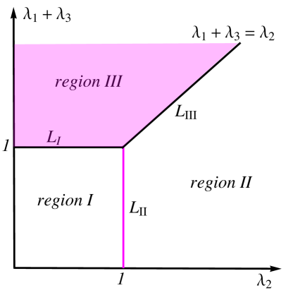
Figure 1. Partitioning of the space of coupling constants $\lambda=(\lambda_{1},\lambda_{2},\lambda_{3})$ for extended Harper’s model. The interesting self-dual regime is colored in red.

The Lyapunov exponents of this model have been determined exactly for all values of parameters:

Theorem 9.9.

[104] Fix an irrational frequency $\alpha$. Then the Lyapunov exponent on the spectrum is zero within both region II and III. In region I it is given by the formula,

(9.7) $$\begin{cases}\log\left(\dfrac{1+\sqrt{1-4\lambda_{1}\lambda_{3}}}{2\lambda_{1}}\right)&\mbox{, if}~{}\lambda_{1}\geq\lambda_{3},~{}\lambda_{2}\leq\lambda_{3}+\lambda_{1}~{}\mbox{,}\\ \log\left(\dfrac{1+\sqrt{1-4\lambda_{1}\lambda_{3}}}{2\lambda_{3}}\right)&\mbox{, if}~{}\lambda_{3}\geq\lambda_{1},~{}\lambda_{2}\leq\lambda_{3}+\lambda_{1}~{}\mbox{,}\\ \log\left(\dfrac{1+\sqrt{1-4\lambda_{1}\lambda_{3}}}{\lambda_{2}+\sqrt{\lambda_{2}^{2}-4\lambda_{1}\lambda_{3}}}\right)&~{}\mbox{, if}~{}\lambda_{2}\geq\lambda_{3}+\lambda_{1}~{}\mbox{.}\end{cases}$$

Computation of the LE for extended Harper’s model was possible using complexification of the phase together with the analytic properties of the complexified LE, $L(E;y)$, see (4.14). The strategy dubbed “method of almost constant cocycles,” relies on the observation that the Jacobi cocycles in the limit $y\to\infty$ are close to a constant cocycle inducing a $\mathcal{DS}$. Since this method allowed to compute the complexified LE, it immediately implied a complete description of the spectral properties in the sense of Avila’s global theory. We mention that these ideas can be used more generally for Jacobi operators with sampling functions given by trigonometric polynomials, e.g. [135] employs it to obtain sufficient criteria for sub-critical behavior for a generalized almost Mathieu operator with potential given by a linear combination of cosines.

Like for the almost Mathieu operator, the spectral theory can now be described fully for all $\lambda$ and almost all $\alpha,\theta:$

Theorem 9.10.

For all Diophantine $\alpha$ for Region I, and for all irrational $\alpha$ for regions II, III, Fig. 2 represents the Lebesgue decomposition of the spectrum of $H_{\theta;\lambda,\alpha}$ for a.e. $\theta$.

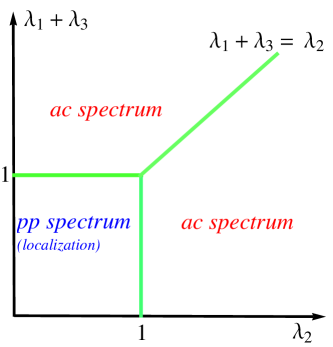
(a) $\lambda_{1}\neq\lambda_{3}$

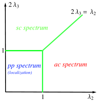
(b) $\lambda_{1}=\lambda_{3}$

Figure 2. Spectral theory of extended Harper’s model. Green indicates (purely) singular continuous spectrum. The spectral properties of extended Harper’s model crucially depend on the symmetry of NNN interaction. Particularly noteworthy is the collapse in the self-dual regime, from purely absolutely continuous spectrum for $\lambda_{1}\neq\lambda_{3}$ to purely singular continuous spectrum once $\lambda_{1}=\lambda_{3}$. Anderson localization in region I had been proven before in [90].

The result for the region I is due to [90], and for the region II,III to [106, 20]. For Liouville $\alpha$ in region I the spectrum is singular continuous [117], but the precise arithmetic transition, like for the almost Mathieu operator, has not yet been explored.

As for the measure of the spectrum, it has been determined as of this writing in the non-self-dual region only. More precisely, let $a\leq b\leq c$ be the ordering of $1,\lambda_{2},\lambda_{1}+\lambda_{3}.$ We have

Theorem 9.11.

[78] For almost all $alpha,$ measure of the spectrum in regions I,II is equal to $4(c-b).$

The Cantor nature of the spectrum has been determined for Diophantine $\alpha$ in regions I, II, moreover:

Theorem 9.12.

[80] For any $\lambda\in I,II,$ if $\beta(\alpha)=0,$ the dry ten martini holds.

The situation so far proves difficult for the remaining parameters.

9.3. The Maryland model

The Maryland model is given by

(9.8) $$(h_{\lambda,\alpha,\theta}u)_{n}=u_{n+1}+u_{n-1}+\lambda\tan\pi(\theta+n\alpha)u_{n}.$$

It was proposed by Grempel, Fishman, and Prange [76] as a model stemming from the study of quantum chaos. In physics it became quite popular as an exactly solvable example of the family of incommensurate models, e.g. [29, 69], with spectral transitions governed by arithmetics. It was dubbed the Maryland model by B. Simon [155, 48] who cited it as a textbook example of dealing with small divisors. Already in the early 80s the spectral theory of the Maryland model has been described for almost all values of $\alpha,\theta$ with arithmetic conditions on $\alpha$ [155, 138]. The region of the transition has been however difficult to handle. Recently, the Maryland model has become the first one for which the spectral decomposition has been determined for all parameters. Define an index $\delta(\alpha,\theta)\in[-\infty,\infty]$,

(9.9) $$\delta(\alpha,\theta)=\limsup_{n\rightarrow\infty}\frac{\ln||q_{n}(\theta-1/2)||_{\mathbb{R}/\mathbb{Z}}+\ln q_{n+1}}{q_{n}},$$

where $||x||_{\mathbb{R}/\mathbb{Z}}=\min_{\ell\in\mathbb{Z}}|x-\ell|$. Let $\gamma_{\lambda}(e)$ be the Lyapunov exponent. remarkably, it is an explicit function, namely the solution of

(9.10) $$4\cosh\gamma_{\lambda}(e)=\sqrt{(2+e)^{2}+\lambda^{2}}+\sqrt{(2-e)^{2}+\lambda^{2}},$$

Let $\sigma_{pp}(h)$, $\sigma_{sc}(h)$ and $\sigma_{ac}(h)$ be the pure point spectrum, singular continuous spectrum, and absolutely continuous spectrum of $h,$ respectively. Assume $\alpha\in\mathbb{R}\backslash\mathbb{Q}$ (otherwise the spectrum is purely absolutely continuous), $\lambda>0$ (otherwise use $h_{\lambda,\alpha,\theta}=h_{-\lambda,-\alpha,-\theta}$) and $\theta\notin 1/2+\alpha\mathbb{Z}+\mathbb{Z}$ (so the potential is well defined).

Theorem 9.13.

[97] For all $\alpha,\lambda,\theta$ as above , we have

1. $\sigma_{sc}(h_{\lambda,\alpha,\theta})=\overline{\{e:\gamma_{\lambda}(e)<\delta(\alpha,\theta)\}}$

2. $\sigma_{pp}(h_{\lambda,\alpha,\theta})=\{e:\gamma_{\lambda}(e)\geq\delta(\alpha,\theta)\}$

3. $\sigma_{ac}(h_{\lambda,\alpha,\theta})=\emptyset.$

The proof is achieved through a new Gordon-type method, that allows to handle singular potentials in a sharp way, as well as a new technique for handling the cohomological equation in the regime of very small denominators.

References

- [1] S. Aubry, G. André, Analyticity breaking and Anderson localization in incommensurate lattices, Ann. Israel Phys. Soc. 3, 133-164 (1980).
- [2] A. Avila and J. Bochi, A formula with some applications to the theory of Lyapunov exponent, Israel J. Math. 131 (2002), 125ミ37.
- [3] A. Avila, D. Damanik, Generic singular spectrum for ergodic Schrödinger operators, Duke Math. J. 130 (2005), 393 - 400.
- [4] A. Avila, S. Jitomirskaya, Almost localization and almost reducibility, Journal of the European Mathematical Society 12 (2010), 93-131.
- [5] A. Avila, R. Krikorian, Reducibility and non-uniform hyperbolicity for quasiperiodic Schrödinger cocycles, Annals of Mathematics 164, 911-940 (2006).
- [6] A. Avila, Absolutely continuous spectrum for the almost Mathieu operator with subcritical coupling, 2008. Preprint available on arXiv:0810.2965v1.
- [7] A. Avila, On point spectrum with critical coupling Preprint available on www.impa.br/ avila/.
- [8] A. Avila, Global theory of one-frequency Schrödinger operators, Acta Math. 215, 1-54 (2015).
- [9] A. Avila, Density of positive Lyapunov exponents for cocycles, Journal of the American Mathematical Society 24 (2011), 999-1014.
- [10] A. Avila, R. Krikorian, Reducibility and non-uniform hyperbolicity for quasiperiodic Schrödinger cocycles, an extended preprint of [5] (2006), available under http://w3.impa.br/avila/
- [11] A. Avila, B. Fayad, R. Krikorian, A KAM scheme for SL(2,) cocycles with Liouvillian frequencies, Geometric and Functional Analysis 21, 1001-1019 (2011).
- [12] A. Avila, R. Krikorian, Monotonic Cocycles, Inventiones math. 202 (1), 271 - 331 (2015).
- [13] A. Avila, S. Jitomirskaya, C. Sadel, Complex one-frequency cocycles, JEMS 16 (9), 1915 - 1935 (2014).
- [14] A. Avila, On the Kotani-Last and Schrödinger conjectures, Journal of the AMS 28, 579-616 (2015).
- [15] A. Avila, Lyapunov exponents, KAM and the spectral dichotomy for one-frequency Schrödinger operators, in preparation.
- [16] A. Avila, Almost reducibility and absolute continuity I, 2011. Preprint available on arXiv:1006.0704v1.
- [17] A. Avila, Almost reducibility and absolute continuity II, in preparation.
- [18] A. Avila, D. Damanik, Absolute continuity of the integrated density of states for the almost Mathieu operator with non-critical coupling, Inventiones 172, 439-453 (2008)
- [19] A. Avila, S. Jitomirskaya, The ten Martini problem, Annals of Mathematics 170, 303-342 (2009).
- [20] A. Avila, S. Jitomirskaya, C. A. Marx, On the spectral theory of Extended Harper’s Model, in preparation (2015).
- [21] A. Avila, S. Jitomirskaya, Q. Zhou, Second phase transition line, preprint.
- [22] A. Avila, J. You, Q. Zhou, Sharp Phase Transitions for the almost Mathieu operator, preprint (2015). Preprint available under arXiv:1512.03124
- [23] A. Avila, J. You, Q. Zhou. Dry ten Martini problem in the non-critical case. In preparation.
- [24] J. Avron, B. Simon, Almost periodic Schrödinger operators. II. The integrated density of states., Duke Math. J. 50 (1983), 369 – 391.
- [25] J. Avron, P. H. M. v. Mouche, and B. Simon, On the Measure of the Spectrum for the Almost Mathieu Operator, Commun. Math. Phys. 132, 103-118 (1990).
- [26] J. Avron, D. Osadchy and R. Seiler, A topological look at the Quantum Hall Effect, Phys. Today 56, 8 (2003), 38 - 42.
- [27] J. Bellissard, The Gap Labelling Theorem: the case of automatic sequences in Quantum and non-commutative analysis (Kyoto, 1992), pp. 179-181, Math. Phys. Stud., 16, Kluwer Acad. Publ., Dordrecht, (1993).
- [28] Y. M. Berezanskii, Expansions in Eigenfunctions of Self-Adjoint Operators, Americ. Math. Soc., Providence (1968).
- [29] M. Berry. Incommensurability in an exactly-soluble quantal and classical model for a kicked rotator. Physica D, 10:369–378, 1984.
- [30] I. Binder and M. Voda, An estimate on the number of eigenvalues of a quasiperiodic Jacobi matrix of size contained in an interval of size , Journal of Spectral Theory 3 (2013), 1 - 45.
- [31] I. Binder and M. Voda, On Optimal Separation of Eigenvalues for a Quasiperiodic Jacobi Matrix, Commun. Math. Phys. 325, 1063–1106 (2014).
- [32] K. Bjerklov, Positive Lyapunov exponent and minimality for a class of one-dimensional quasi-periodic Schrödinger equations, Ergodic Theory Dynam. Systems 25 (2005), 1015 - 1045.
- [33] J. Bochi, Genericity of zero Lyapunov exponents, Ergodic Theory Dynam. Systems, 22(6) (2002), 1667-1696.
- [34] J. Bochi and M. Viana, The Lyapunov exponents of generic volume-preserving and symplectic maps, Annals of Mathematics 161 (2005), 1423 - 1485.
- [35] M. Boshernitzan, D. Damanik, Generic continuous spectrum for ergodic Schrödinger operators, Commun. Math. Phys. 283 (2008), 647 - 662.
- [36] J. Bourgain, Green’s function estimates for lattice Schr單inger operators and applications, Princeton Univ. Press (2005), Princeton.
- [37] J. Bourgain, Positivity and continuity of the Lyapunov exponent for shifts on with arbitrary frequency vector and real analytic potential, Journal d’Analyse Mathématique 96 (2005), 313 - 355.
- [38] J. Bourgain, M. Goldstein, On nonperturbative localization with quasi-periodic potential, Annals of Mathematics 152 (2000), 835 - 839.
- [39] J. Bourgain, A. Klein, Bounds on the density of states for Schrödinger operators, Invent. math. 194 (2013), 41 - 72.
- [40] J. Bourgain, S. Jitomirskaya, Anderson localization for the band model, Lecture Notes in Math. 1745, 67-79, Springer, Berlin, 2000.
- [41] J. Bourgain, S. Jitomirskaya, Continuity of the Lyapunov exponent for quasi-periodic operators with analytic potential, J. Statist. Phys. 108 (2002), no. 5-6, 12031218.
- [42] J. Bourgain, S. Jitomirskaya, Absolutely continuous spectrum for 1D quasiperiodic operators, Invent. math. 148 (2002), 453 - 463.
- [43] J. Chan, M. Goldstein, W. Schlag, On non-perturbative Anderson localization for potentials generated by shifts and skew-shifts, preprint (2006). Preprint available on arXiv:math/06077302v2 [math.DS].
- [44] M.D. Choi, G.A.Eliott, N. Yui, Gauss polynomials and the rotation algebra. Invent. Math. 99, 225-246 (1990).
- [45] V. Chulaevsky, F. Delyon, Purely absolutely continuous spectrum for almost Mathieu operators., J. Statist. Phys. 55 (1989), 1279 – 1284.
- [46] W. Craig, Point spectrum for discrete almost periodic Schrödinger operators, Commun. Math. Phys. 88 (1983), 113 - 131.
- [47] W. Craig and B. Simon, Subharmonicity of the Lyapunov Index, Duke Mathematical Journal 50 (1983), 551 - 560.
- [48] H. Cycon, R. Froese, W. Kirsch, and B. Simon, Schrödinger Operators with Application to Quantum Mechanics and Global Geometry, Texts and Monographs in Physics, Springer-Verlag, Berlin, (1987).
- [49] D. Damanik, Lyapunov Exponent and spectral analysis of ergodic Schrödinger operators: A survey of Kotani theory and its applications, Spectral Theory and Mathematical Physics: A Festschrift in Honor of Barry Simon’s 60th Birthday, Proceedings of Symposia in Pure Mathematics 76 Part 2, American Mathematical Society, Providence, 2007.
- [50] D. Damanik, M. Goldstein, W. Schlag, M. Voda Homogeneity of the spectrum for quasi-perioidic Schrödinger operators. Preprint http://arxiv.org/pdf/1505.04904
- [51] D. Damanik, R. Killip, Ergodic potentials with a discontinuous sampling function are non-deterministic, Math. Research Letters 12 (2005) 187-193.
- [52] D. Damanik, R. Killip, B. Simon, Perturbations of orthogonal polynomials with periodic recursion coefficients, Annals of Math. 171 (2010), 1931-2010.
- [53] D. Damanik, Schrödinger Operators with Dynamically Defined Potentials: A Survey, Ergodic Theory and Dynamical Systems, to appear.
- [54] D. Damanik, S. Tcheremchantzev, Upper bounds in quantum dynamics. JAMS 20, 799-827 (2007)
- [55] P. Deift and B. Simon, Almost periodic Schrödinger operators, III. The absolutely continuous spectrum in one dimension, Commun. Math. Phys. 90 (1983), 389-411.
- [56] F. Delyon, Absence of localization for the almost Mathieu equation. J.Phys. A 20, L21-L23 (1987).
- [57] F. Delyon, B. Souillard, The rotation number for finite difference operators and its properties, Commun. Math. Phys. 89 (1983), 415 - 426.
- [58] F. Delyon, B. Souillard, Remark on the Continuity of the Density of States of Ergodic Finite Difference Operators, Commun. Math. Phys 94 (1984), 289 - 291.
- [59] E. I Dinaburg abd Ya. G. Sinai, The one-dimensional Schrödinger equation with a quasi-periodic potential, Funct. Anal. Appl. 9 (1975), 279 - 289.
- [60] M. Disertori, W. Kirsch, A. Klein, F. Klopp, V. Rivasseau, Random Schrödinger Operators, Panoramas et Syntheses 25 (2008).
- [61] J. Dombrowsky, Quasitriangular matrices, Proc. Amer. Math. Soc. 69 (1978), 95-96.
- [62] P. Duarte and S. Klein, Continuity of the Lyapunov exponents for quasi-periodic cocycles, Commun. Math. Phys. 332, 1113-1166 (2014)
- [63] P. Duarte and S. Klein, Positive Lyapunov exponents for higher dimensional quasiperiodic cocycles, Commun. Math. Phys. 332, 189-219 (2014)
- [64] P. L. Duren, Theory of spaces, Pure and Applied Mathematics, Vol. 38, Academic Press, New York 1970.
- [65] L. H. Eliasson, Floquet Solutions for the 1-dimensional quasi-periodic Schrödinger equation, Commun. Math. Phys. 146 (1982), 447 - 482.
- [66] L. H. Eliasson, Discrete one-dimensional quasi-periodic Schrödinger operators with pure point spectrum. Acta Math. 179, 153–196 (1997).
- [67] J. Fröhlich, T. Spencer, P. Wittwer, Localization for a class of one dimensional quasi-periodic Schrödinger operators, Commun. Math. Phys. 132 (1990), 5 - 25.
- [68] A. Furman, On the multiplicative ergodic theorem for uniquely ergodic systems, Ann. Inst. Henri Poincaré 33 (1997), no. 6, 797 - 815.
- [69] S. Ganeshan, K. Kechedzhi, and S. Das Sarma. Critical integer quantum hall topology and the integrable maryland model as a topological quantum critical point. Phys. Rev. B, 90:041405, 2014.
- [70] I. Ya. Goldsheid and E. Sorets, Lyapunov Exponents of the Schrödinger Equation with Quasi-Periodic Potential on a Strip, Commun. Math. Phys. 145 (2012), 507 - 513.
- [71] M. Goldstein, W. Schlag, Hölder continuity of the integrated density of states for quasi-periodic Schrödinger equations and averages of shifts of subharmonic functions, Annals of Mathematics 154 (2001), 155- 203.
- [72] M. Goldstein and W. Schlag, Fine properties of the integrated density of states and a quantitative separation property of the Dirichlet eigenvalues, GAFA 18, 765-869 (2008)
- [73] M. Goldstein, W. Schlag, On resonances and the formation of gaps in the spectrum of quasi-periodic Schroedinger equations, Annals of Math 173, 337-475 (2011).
- [74] A. Gordon, The point spectrum of the one-dimensional Schrödinger operator, Uspehi Mat. Nauk 31 (1976), 257 – 258.
- [75] A.Y. Gordon, S. Jitomirskaya, Y. Last and B. Simon, Duality and singular continuous spectrum in the almost Mathieu equation, Acta Mathematica 178 (1997), 169 – 183.
- [76] D. Grempel, S. Fishman, and R. Prange. Localization in an incommensurate potential: An exactly solvable model. Physical Review Letters, 49(11):833, 1982.
- [77] S. Hadj Amor, Hölder continuity of the rotation number for quasi-periodic co-cycles in , Commun. Math. Phys. 287 (2009), 565 - 588.
- [78] R. Han and S. Jitomirskaya, The total bandwidth of the extended Harper’s model. In preparation
- [79] R. Han and S. Jitomirskaya, In preparation.
- [80] R. Han, Dry ten martini problem for the non-self-dual extended Harper’s model. Preprint.
- [81] A. Haro and J. Puig, A Thouless formula and Aubry duality for long-range Schrödinger skew-products, Nonlinearity 26 (2013), 1163 - 1187.
- [82] P. G. Harper, Single band motion of conducting electrons in a uniform magnetic field, Proc. Phys. Soc. A 68 (1955), 874-878.
- [83] M. Herman, Une methode pour minorer les exposants des Lyapunov et quelques examples montrant le charactère local d’un théorème d’Arnold et de Moser sur le tore de dimension 2, Comment. Math. Helv. 58 (1983), 453 - 562.
- [84] D. R. Hofstadter, Energy levels and wave functions of Bloch electrons in rational and irrational magnetic fields, Phys. Rev. B 14, 2239 - 2249 (1976).
- [85] S. Jitomirskaya, Almost everything about the almost Mathieu operator. II. In D. Iagolnitzer, International Congress of Mathematical Physics. Proceedings. International press, Cambridge, MA, 1995, 373-382.
- [86] S. Jitomirskaya, Metal-Insulator transition for the almost Mathieu operator. Annals of Math. 150, 1159-1175 (1999).
- [87] S. Jitomirskaya, B. Simon, Operators with singular continuous spectrum: III. Almost Periodic Schrödinger Operators, Commun. Math. Phys. 165 (1994), 201-205.
- [88] S. Ya. Jitomirskaya, Metal-insulator transition for the almost Mathieu operator, Annals of Mathematics 150 (1999), 1159 - 1175.
- [89] S. Jitomirskaya, Ergodic Schrödinger Operators (on one foot), Proceedings of Symposia in Pure Mathematics 76 (2007), 613 - 647.
- [90] S. Jitomirskaya, D.A. Koslover, M.S. Schulteis, Localization for a family of one-dimensional quasiperiodic operators of magnetic origin, Ann. Henri Poincare 6 , 103–124 (2005).
- [91] S. Jitomirskaya and I. Kachkovskiy, Anderson localization for discrete 1D quaziperiodic operators with piecewise monotonic sampling functions, Preprint 2015.
- [92] S. Jitomirskaya and I. Kachkovsky, -reducibility and localization for quasiperiodic operators, Math. Res. Lett., to appear.
- [93] S. Jitomirskaya and I. Krasovsky, Continuity of the measure of the spectrum for discrete quasiperiodic operators, Math. Res. Letters 9, 413–421 (2002).
- [94] S. Jitomirskaya and H. Krüger, Exponential Dynamical Localization for the Almost Mathieu Operator, Comm. Math. Phys. 322, 877-882 (2013).
- [95] S. Jitomirskaya, H. Krüger, W. Liu, in preparation.
- [96] S. Jitomirskaya and Y. Last, Power-Law Subordinacy and Singular Spectra, II. Line Operators. Comm. Math. Phys., 211, 643-658 (2000).
- [97] S. Jitomirskaya and W. Liu, Arithmetic Spectral Transitions for the Maryland model, Preprint 2014.
- [98] S. Jitomirskaya and W. Liu, Asymptotics of quasiperiodic eigenfunctions. Preprint.
- [99] S. Jitomirskaya and W. Liu, Asymptotics of quasiperiodic eigenfunctions, II. Preprint.
- [100] S. Jitomirskaya, W. Liu, S. Tcheremchancev, in preparation.
- [101] S. Jitomirskaya, C. A. Marx, Continuity of the Lyapunov exponent for analytic quasi-periodic cocycles with singularities, Journal of Fixed Point Theory and Applications 10, 129 -146 (2011)
- [102] S. Jitomirskaya, C. A. Marx, Analytic Quasi-periodic Schrödinger Operators and Rational Frequency Approximation, Geom. Funct. Anal. 22 (2012), 1407 - 1443.
- [103] S. Jitomirskaya, R. Mavi, Continuity of the measure of the spectrum for quasiperiodic Schrödinger operators with rough potentials, Commun. Math. Phys. 325 585-601 (2014)
- [104] S. Jitomirskaya, C. A. Marx, Analytic quasi-perodic cocycles with singularities and the Lyapunov Exponent of Extended Harper’s Model, Commun. Math. Phys. 316, 237-267 (2012).
- [105] S. Jitomirskaya, C. A. Marx, Erratum to: Analytic quasi-perodic cocycles with singularities and the Lyapunov Exponent of Extended Harper’s Model, Commun. Math. Phys. 317, 269-271 (2013).
- [106] S. Jitomirskaya, C. A. Marx, Spectral Theory for Extended Harper’s Model, preprint, 2013.
- [107] S. Jitomirskaya, R. Mavi, Dynamical bounds for quasiperiodic Schrödinger operators with rough potentials, preprint (2015). Preprint available under arXiv:1412.0309
- [108] S. Jitomirskaya, S. Zhang, Quantitative continuity of singular continuous spectral measures and arithmetic criteria for quasiperiodic Schrödinger operators, preprint (2015). Preprint available under arXiv:1510.07086 [math.SP]
- [109] S. Jitomirskaya, Q. Zhou, In preparation.
- [110] R. A. Johnson, Exponential Dichotomy, Rotation Number, and Linear Differential Operators with Bounded Coefficients, Journal of Differential Equations 61 (1986), 54 - 78.
- [111] R. Johnson and J. Moser, The rotation number for almost periodic potentials, Commun. Math. Phys. 84 (1982), 403 - 438.
- [112] W. Kirsch, F. Martinelli, On the ergodic properties of the spectrum of general random operators, J. Reine Angew. Math. 334, 141 - 156 (1982).
- [113] W. Kirsch, An invitation to random Schrödinger operators, arXiv:0709.3707 [math-ph] (2007).
- [114] A. Klein, A. Koines, M. Seifert, Generalized Eigenfunctions for Waves in Inhomogeneous Media, Journal of Functional Analysis 190, 255 - 291.
- [115] S. Klein, Anderson localization for the discrete one-dimensional quasi-periodic Schrödinger operator with potential defined by a Gevrey-class function, Journal of Functional Analysis 218 (2005), 255 - 292.
- [116] S. Klein, Localization for quasi-periodic Schrödinger operators with multivariable Gevrey potential functions, J. Spectr. Theory 4 (2014), no. 3, 431- 484.
- [117] D. A. Koslover, Jacobi Operators with Singular Continuous Spectrum, Letters in Mathematical Physics 71 (2005), 123 - 134.
- [118] S. Kotani, Lyapunov indices determine absolutely continuous spectra of stationary random one- dimensional Schrödinger operators, Proc. Kyoto Stoch. Conf. (1982).
- [119] S. Kotani, B. Simon, Stochastic Schrödinger operators and Jacobi Matrices on the strip, Commun. Math. Phys. 119 (1988), 403 - 429.
- [120] S. Kotani, Generalized Floquet Theory for Stationary Schrödinger Operators in One Dimension, Chaos, Solutions & Fractals 8 (1997), 1817 - 1854.
- [121] I. Krasovsky, Bloch electron in a magnetic field and the Ising model, Phys. Rev. Lett. 85 (2000), 4920 - 4923.
- [122] H. Krüger, G. Zheng, Optimality of log Hölder continuity of the integrated density of states, Math. Nachr. 284 (2011),1919 - 1923.
- [123] H. Kunz, Souillard B., Sur le spectre des opérateurs aux différences finies aléatoires, Commun. Math. Phys. 78, 201 - 246 (1980).
- [124] Y. Last, A relation between absolutely continuous spectrum of ergodic Jacobi matrices and thespectra of periodic approximants, Commun. Math. Phys. 151, 183-192 (1993).
- [125] Y. Last, Zero measure spectrum for the almost Mathieu operator, Commun. Math. Phys. 164, 421-432 (1994).
- [126] Y. Last, Spectral theory of Sturm-Liouville operators on infinite intervals: a review of recent developments. Sturm-Liouville theory, 99–120, Birkhauser, Basel (2005).
- [127] Y. Last, B. Simon, Eigenfunctions, transfer matrices, and absolutely continuous spectrum of one-dimensional Schrödinger operators, Invent. math. 135 (1999), 329-367.
- [128] Y. Last, M. Shamis, Zero Hausdorff dimension spectrum for the almost Mathieu operator, preprint. Preprint available under arXiv:1510.07651
- [129] W. Liu and X. Yuan, Anderson Localization for the Almost Mathieu Operator in Exponential Regime, JST, to appear
- [130] J. M. Luttinger, The effect of a magnetic field on electrons in a periodic potential, Phys. Rev. 84 (1951), 814-817.
- [131] V.A. Mandel’shtam, S. Ya. Zhitomirskaya, 1D-Quaisperiodic Operators. Latent Symmetries, Commun. Math. Phys. 139 (1991), 589 - 604.
- [132] C. A. Marx, Quasi-periodic Jacobi-cocycles: Dynamics, Continuity, and Applications to Extended Harper’s Model, PhD thesis, Irvine, CA (2012).
- [133] C. A. Marx, Dominated splittings and the spectrum for quasi periodic Jacobi operators, Nonlinearity 27, 3059-3072 (2014).
- [134] J. Moser and J. Pöschel, An extension of a result by Dinaburg and Sinai on quasi-periodic potentials, Comment. Math. Helvetici 59 (1984), 39 - 85.
- [135] C. A. Marx, L. Shou, and J. Wellens, A sufficient criterion of subcritical behavior in quasi-periodic Jacobi operators with trigonometric sampling functions, Journal of Spectral Theory, to appear.
- [136] V. I. Oseledets, A multiplicative ergodic theorem. Ljapunov characteristic numbers for dynamical systems, Trudy Moskov. Mat. Obšč. 19 (1968), 179 - 210. English transl. Trans. Moscow Math Soc. 19 (1968), 197 - 231.
- [137] L. Pastur, Spectral properties of disordered systems in one-body approximation, Commun. Math. Phys 75 (1980), 179.
- [138] A. L. Figotin and L. A. Pastur. An exactly solvabl emodel of a multidimensional incommensurate structure. Comm. Math. Phys., 95(4):401–425, (1984).
- [139] L. Pastur and A. Figotin, Spectra of Random and Almost-Periodic Operators, Grundlehren der Mathematischen Wissenschaften [Fundamental Principles of Mathematical Sciences], 297, Springer-Verlag, Berlin, 1992.
- [140] R. Peierls, Z. Physik 80 (1933), 763.
- [141] J. Pöschel, Examples of discrete Schrödinger operators with pure point spectrum, Commun. Math. Phys. 88 (1983), 447 - 463.
- [142] J. Puig, Cantor spectrum for the almost Mathieu operator, Comm. Math. Phys. 244, 297–309 (2004).
- [143] J. Puig, A nonperturbative Eliasson’ s reducibility theorem, Nonlinearity 19 (2006), 355 - 376.
- [144] A. Rauh, Degeneracy of Landau levels in crystals, Phys. Status Solidi B 65, K131-135 (1974).
- [145] D. Ruelle, Ergodic theory of differentiable dynamical systems, Publications Mathématiques de l’IHÉs 50 (1979), 27 - 58.
- [146] D. Ruelle, Analyticity Properties of the Characteristic Exponents of Random Matrix Products, Advances in Mathematics 32 (1979), 68-80.
- [147] W. Schlag, Regularity and convergence rate for the Lyapunov exponents of linear cocycles, Journal of modern Dynamics 7(2013), 619 - 637.
- [148] I. Sch’nol, On the behavior of the Schrödinger equation, Mat. Sb. 42 (1957), 273-286.
- [149] M. Shamis, Spectral analysis of Jacobi operators, PhD Thesis, Hebrew University of Jerusalem, 2010.
- [150] M. Shamis, Th. Spencer, Bounds on the Lyapunov exponent via crude estimates on the density of states, Comm. Math. Phys. 338 (2015), no. 2, 705–720.
- [151] B. Simon, Almost Periodic Schrd̈inger Operators: A Review, Adv. in Applied Math. 3 (1982), 463 - 490.
- [152] B. Simon, Schrödinger semigroups, Bull. Amer. Math. Soc. 7 (1982), 447 - 526.
- [153] B. Simon, Kotani Theory for one dimensional stochastic Jacobi matrices, Commun. Math. Phys. 89 (1983), 227 - 234.
- [154] B. Simon, Fifteen problems in mathematical physics, Oberwolfach Anniversary Volume (1984), 423-454.
- [155] B. Simon. Almost periodic Schrödinger operators. IV. The Maryland model. Ann. Physics, 159(1):157– 183, 1985.
- [156] B. Simon, Schrödinger operators in the twenty-first century, Mathematical physics 2000, 283–288, Imp. Coll. Press, London, 2000.
- [157] B. Simon, Orthogonal Polynomials on the Unit Circle. Part 2: Spectral Theory, American Mathematical Society Colloquium Publications 54, Providence, 2005.
- [158] B. Simon,Equilibrium measures and capacities in spectral theory, Inverse Problems and Imaging 1 (2007), 713-772
- [159] Ya. Sinai, Anderson localization for one-dimensional difference Schrödinger operator with quasi-periodic potential, J. Stat. Phys. 46 (1987), 861 - 909.
- [160] E. Sorets, T. Spencer, Positive Lyapunov Exponents for Schrödinger Operators with quasi-periodic potentials, CMP 142 (3), 543 - 566 (1991).
- [161] T. Spencer, Ergodic Schr¨odinger operators, Analysis, et cetera, 623–637, Academic Press, Boston, MA, 1990.
- [162] G. Teschl, Jacobi Operators and Completely Integrable Nonlinear Lattices, Mathematical Surveys and Monographs 72, Amer. Math. Soc., Providence (2000).
- [163] D.Thouless, A relation between the density of states and range of localization for one-dimensional random system, J. Phys. C 5 (1972), 77 - 81.
- [164] D. J. Thouless, Bandwidth for a quasiperiodic tight binding model, Phys. Rev. B 28, 42724276 (1983).
- [165] D. J. Thouless, M. Kohmoto, M. P. Nightingale, and M. den Nijs, Quantized Hall Conductance in a Two-Dimensional Periodic Potential, Phys. Rev. Lett. 49 (1982), 405 - 408.
- [166] K. Tao, Hölder continuity of Lyapunov exponent for quasi-periodic Jacobi operators, Bulletin de la Société mathématique de France 142 (4), 635 - 671 (2014).
- [167] K. Tao, Continuity of Lyapunov exponent for analytic quasi-periodic cocycles on higher-dimensional torus, Front. Math. China (2012), 521 - 542.
- [168] K. Tao, M. Voda, Hölder continuity of the integrated density of states for quasi-periodic Jacobi operators, preprint (2015). Preprint available on arXiv:1501.01028 [math.SP].
- [169] Y. Wang and J. You, Examples of discontinuity of Lyapunov Exponent in smooth quasi-periodic cocycles, Duke Math J. 162 No. 13, 2363 - 2412.
- [170] Y. Wang and J. You, Quasi-Periodic Schr dinger Cocycles with Positive Lyapunov Exponent are not Open in the Smooth Topology, preprint 2015. Preprint available on arXiv:1501.05380
- [171] Y. Wang and Z. Zhang, Uniform positivity and continuity of Lyapunov exponents for a class of quasiperiodic Schrödinger cocycles, J. Funct. Anal. 268, 2525-2585 (2015).
- [172] Y. Wang and Z. Zhang, Cantor spectrum for a class of quasiperiodic Schrödinger operators, to appear in Int. Math. Res. Notices.
- [173] J. You and Q. Zhou, Embedding of analytic quasi-periodic cocycles into analytic quasi-periodic linear systems and its applications, Commun Math Phys. 323, 975-1005 (2013).
- [174] L.-S. Young, Lyapunov exponents for some quasi-periodic cocycles, Ergod. Th. & Dynam. Sys. 17, 483-504 (1997).
- [175] Z. Zhang, Resolvent set of Schrödinger operators and uniform hyperbolicty, preprint (2013). Preprint available on arXiv:1305.4226v1.
- [176] Z. Zhang, Positive lyapunov exponents for quasiperiodic Szegő cocycles, Nonlinearity 25 (2012), 1771 - 1797.