Cost-Effective Conceptual Design Using Taxonomies

Abstract

It is known that annotating named entities in unstructured and semi-structured data sets by their concepts improves the effectiveness of answering queries over these data sets. Ideally, one would like to annotate entities of all concepts in a given domain in a data set, however, it takes substantial time and computational resources to do so over a large data set. As every enterprise has a limited budget of time or computational resources, it has to annotate a subset of concepts in a given domain whose costs of annotation do not exceed the budget. We call such a subset of concepts a conceptual design for the annotated data set. We focus on finding a conceptual design that provides the most effective answers to queries over the annotated data set, i.e., a cost-effective conceptual design. Since, it is often less time-consuming and costly to annotate small number of general concepts, such as person, than a large number of specific concepts, such as politician and artist, we use information on superclass/ subclass relationships between concepts in taxonomies to find a cost-effective conceptual design. We quantify the amount by which a conceptual design with concepts from a taxonomy improves the effectiveness of answering queries over an annotated data set. If the taxonomy is a tree, we prove that the problem is NP-hard and propose an efficient approximation algorithm and an exact pseudo-polynomial time algorithm for the problem. We further prove that if the taxonomy is a directed acyclic graph, given some generally accepted hypothesis, it is not possible to find any approximation algorithm with reasonably small approximation ratio or a pseudo-polynomial algorithm for the problem. Our empirical study using real-world data sets, taxonomies, and query workloads shows that our framework effectively quantifies the amount by which a conceptual design improves the effectiveness of answering queries. It also indicates that our algorithms are efficient for a design-time task with pseudo-polynomial algorithm being generally more effective than the approximation algorithm.

1 Introduction

1.1 Concept Annotation

Unstructured and semi-structured data sets, such as HTML documents, contain enormous information about named entities like people and products [9, 12]. Users normally explore these data sets using keyword queries to find information about their entities of interest. Unfortunately, as keyword queries are generally ambiguous, query interfaces may not return the relevant answers for these queries. For example, consider the excerpts of the Wikipedia
(wikipedia.org) articles in Figure 1. Assume that a user likes to find information about John Adams, the politician, over this data set. If she submits query $Q_{1}$:John Adams, the query interface may return the articles about John Adams, the artist, or John Adams, the school, as relevant answers. Users can further disambiguate their queries by adding appropriate keywords. Nonetheless, it is not easy to find such keywords [32]. For instance, if one refines $Q_{1}$ to John Adams Ohio, the query interface may return the article about John Adams, the high school, as the answer. It will not help either to add keyword Congressman to $Q_{1}$ as this keyword does not appear in the article about John Adams, the politician. Formulating the appropriate keyword query requires some knowledge about the sought after entity and the data that most users do not usually possess.

<article>
 John Adams has been a former member of the Ohio House of
 Representatives from 2007 to 2014. ...
</article>
<article>
 John Adams is a composer whose music is inspired by nature, ...
</article>
<article>
 John Adams is a public high school located on the east side of
 Cleveland, Ohio, ...
</article>

Figure 1: Wikipedia article excerpts

<article>
 <politician> John Adams </politician> has been a former member
 of the <legislature> Ohio House of Representatives </legislature>
 from 2007 to 2014. ...
</article>
<article>
 <artist> John Adams </artist> is a composer whose music is inspired
 by nature, ...
</article>
<article>
 <school> John Adams </school> is a public high school located on
 the east side of <city>Cleveland</city>, <state>Ohio</state>, ...
</article>

Figure 2: Annotated Wikipedia article excerpts

To make querying unstructured and semi-structured data sets easier, data management researchers have proposed methods to identify the mentions to entities in these data sets and annotate them by their concepts [9, 12]. Figure 2 shows excerpts of the annotated Wikipedia articles whose original versions are shown in Figure 1. Because entities in an annotated data set are disambiguated by their concepts, the query interface can answer queries over these data sets more effectively. Moreover, as the list of concepts used to annotate the data sets are available to users, they can further clarify their queries by mentioning the concepts of entities in these queries. For example, a user who would like to retrieve article(s) about John Adams, the politician, over the annotated Wikipedia data set in Figure 2 may mention the concept of politician in her query. The set of annotated concepts in a data set is the conceptual design for the data set [28]. For example, the conceptual design of the data fragment in Figure 2 is $D_{1}$ = {politician, legislature, artist, school, state, city}. Using $D_{1}$, the query interface is able to disambiguate all entities in this data fragment.

1.2 Costs of Concept Annotation

Ideally, an enterprise would like to annotate all relevant concepts from a data set to answer all queries effectively. Nonetheless, an enterprise has to spend significant time, financial and computational resources, and manual labor to accurately extract entities of a concept in a large data set [4, 17, 9, 28, 20, 27, 18, 21]. An enterprise usually has to develop or obtain a complex program called concept annotator to annotate entities of a concept from a collection of documents [24]. Enterprises develop concept annotator using rule-based or machine learning approaches. In the rule-based approach, developers have to design and write hand-tuned programming rules to identify and annotate entities of a given concept. For example, one rule to annotate entities of concept person is that they start with a capital letter. It is not uncommon for a rule-based concept annotator to have thousands of programming rules, which takes a great deal of resources to design, write, and debug [24].

One may also use machine learning algorithms to develop an extractor for a concept [24]. In this approach, developers have to find a set of relevant features for the learning algorithm. Unfortunately, as the specifications of relevant features are usually unclear, developers have to find the relevant features through a time-consuming and labor-intensive process [4, 3]. First, they have to inspect the data set to find some candidate features. For each candidate feature, developers have to write a program to extract the value(s) of the feature from the data set. Finally, they have to train and test the concept annotator using the set of selected features. If the concept annotator is not sufficiently accurate, developers have to explore the data set for new features. As a concept annotator normally uses hundreds of features, developers have to iterate these steps many times to find a set of reasonably effective features, where each iteration usually takes considerable amount of time [4, 3]. The overheads feature engineering and computation have been well recognized in machine learning community [30]. Moreover, if concept annotators use supervised learning algorithms, developers have to collect or create training data, which require additional time and manual labor.

It is more resource-intensive to develop annotators for concepts in specific domains, such as biology, as it requires expensive communication between domain experts and developers. Current studies indicate that these communications are not often successful and developers have to slog through the data set to find relevant features for concept annotators in these domains [4].

Unfortunately, the overheads of developing a concept annotator are not one-time costs. Because the structure and content of underlying data sets evolve over time, annotators should be regularly rewritten and repaired [17]. Recent studies show that many concept annotator need to be rewritten in average about every two months [17]. Thus, the enterprise often have to repeat the resource-intensive steps of developing a concept annotator to maintain an up-to-date annotated data set.

After developing concept annotators, the enterprise executes them over the data set to generate the annotated collection. As most concept annotators perform complex text analysis, such as deep natural language parsing, it may take them days to process a large data set [20, 27, 18, 21]. As the content of the data set evolves, extractors should be often rerun to create an updated annotated collection.

1.3 Cost-Effective Conceptual Design

Figure 3: Fragments of DBpedia taxonomy from dbpedia.org

<article>
 <person> John Adams </person> has been a former member
 of the <organization> Ohio House of Representatives </organization>
 from 2007 to 2014. ...
</article>
<article>
 <person> John Adams </person> is a composer whose music is inspired
 by nature, ...
</article>
<article>
 <organization> John Adams </organization> is a public high school
 located on the east side of <city>Cleveland</city>, <state>Ohio</state>,
 ...
</article>

Figure 4: Wikipedia article excerpts organized in more general concepts

Because the available financial or computational resources of an enterprise are limited, it may not afford to develop, deploy, and maintain annotators for all concepts in a domain. Also, many users may need an annotated data set quickly and cannot wait days for an (updated) annotated collection [27, 20]. For example, a reporter who pursues some breaking news, a stock broker that studies the relevant news and documents about companies, and an epidemiologist that follows the pattern of a new potential pandemic on the Web and social media need relevant answers to their queries fast. Hence, the enterprise may afford to annotate only a subset of concepts in a domain.

Concepts in many domains are organized in taxonomies [1]. Figure 3 depicts fragments of DBPedia dbpedia.org taxonomy, where nodes are concepts and edges show superclass/ subclass relationships. An enterprise can use the information in a taxonomy to find a conceptual design whose associated costs do not exceed its budget and deliver reasonably effective answers for queries. For example, assume that because an enterprise has to develop in-house annotators for concepts politician and artist, the total cost of annotating concepts in conceptual design $D_{1}$ = {politician, artist, legislature, school, state, city} over original Wikipedia collection exceeds its budget. As some free and reasonably accurate annotators are available for concept person,
e.g. nlp.stanford.edu/software/CRF-NER.shtml, the enterprise may annotate concept person using smaller amount of resources than concepts politician and artist. Hence, it may afford to annotate concepts $D_{2}$ = {person, organization, state, city} from this collection. Thus, the enterprise may choose to annotate the data set using $D_{2}$ instead of $D_{1}$. Figure 4 demonstrates the annotated version of the excerpts of Wikipedia articles in Figure 1 using conceptual design $D_{2}$.

Intuitively, a query interface can disambiguate fewer queries over the data fragment in Figure 4 than the one in Figure 2. For instance, if a users ask for information about John Adams, the politician, over Figure 4, the query interface may return the document that contains information about John Adams, the artist, as an answer as both entities are annotated as person. Nonetheless, the annotated data set in Figure 4 can still help the query interface to disambiguate some queries. For example, the query interface can recognize the occurrence of entity John Adams, the school, from the people named John Adams in Figure 4. Thus, it can answer queries about the school entity over this data fragment effectively. Clearly, an enterprise would like to select a conceptual design whose required time and/or resources for extraction do not exceed its budget and most improves the effectiveness of answering queries. We call such a conceptual design for an annotated data set, a cost-effective conceptual design for the data set.

1.4 Our Contributions

Currently, concept annotation experts use their intuitions to discover cost-effective conceptual designs from taxonomies. Because most taxonomies contain hundreds of concepts [15], this approach does not scale for real-world applications. In this paper, we introduce and formalize the problem of finding cost-effective conceptual designs from taxonomies and propose algorithms to solve the problem in general and interesting special cases. To this end, we make the following contributions.

• We develop a theoretical framework that quantifies the amount of improvement in the effectiveness of answering queries by annotating a subset of concepts from a taxonomy. Our framework takes into account possibility of error in concept annotation.

• We introduce and formally define the problem of cost-effective conceptual design over tree-shaped taxonomies and show it to be NP-hard.

• We propose an efficient approximation algorithm, called the level-wise algorithm, and prove that it has a bounded worst-case approximation ratio in an interesting special case of the problem. We also propose an exact algorithm for the problem with pseudo polynomial running time.

• We further define the problem over taxonomies that are directed acyclic graphs and prove that given a generally accepted hypothesis, there is no approximation algorithm with reasonably small approximation ratio and no algorithm with pseudo polynomial running time for this problem. We show that these results hold even for some restricted cases of the problem, such as the case where all concepts are equally costly.

• We evaluate the accuracy of our formal framework using a large scale real-world data set, Wikipedia, real-world taxonomies [15], and a sample of a real-world query workload. Our results indicate that the formal framework accurately measures the amount of improvement in the effectiveness of answering queries using a subset of concepts from a taxonomy.

• We perform extensive empirical studies to evaluate the accuracy and efficiency of the proposed algorithms over real-world data sets, taxonomies, and query workload. Our results indicate that the pseudo polynomial algorithm is generally able to deliver more effective schemas that the level-wise algorithm in reasonable amounts of time. They further show that level-wise algorithm provides more effective conceptual designs than the pseudo polynomial algorithm if the distribution of concepts in queries is skewed.

The paper is organized as follows. Section 2 reviews the related work. Section 3 formalizes the problem of cost-effective conceptual design over a tree-shaped taxonomy and show that it is NP-hard. Section 4 describes an efficient approximation algorithm with bounded approximation ratio in an interesting special case of the problem. Section 5 proposes a pseudo-polynomial algorithm for the problem in general case. Section 6 defines the problem over taxonomies that are directed acyclic graphs and provides interesting hardness results for this setting. Section 8 concludes the paper. The proofs for the theorems of the paper are in the appendix.

2 Related Work

Researchers have noticed the overheads and costs of curating and organizing large data sets [13, 21, 20]. For example, some researchers have recently considered the problem of selecting data sources for fusion such that the marginal cost of acquiring a new data source does not exceed its marginal gain, where cost and gain are measured using the same metric, e.g., US dollars [13]. Our work extends this line of research by finding cost-effective designs over unstructured or semi-structured data sets, which help users query explore these data sets more easily. We also use a different model, where the cost and benefit of annotating concepts can be measured in different units.

There is a large body of work on building large-scale data management systems for annotating and extracting entities and relationships from unstructured and semi-structured data sources [9, 12]. In particular, researchers have proposed several techniques to optimize the running time, required computational power, and/or storage consumption of concept annotation programs by processing only a subset of the underlying collection that is more likely to contain mentions to entities of a given concept [19, 20, 18, 21]. Our work complements these efforts by finding a cost-effective set of concepts for annotation in the design phase. Further, our framework can handle other types of costs in creating and maintaining annotated data set other than computational overheads.

Researchers have examined the problem of selecting a cost effective subset of concepts from a set of concepts for annotation [28]. Concepts in many real-world domains, however, are maintained in taxonomies rather than unorganized sets. We build on this line of work by considering the superclass/ subclass relationships between concepts in taxonomies to find cost-effective designs. Because taxonomies have richer structures than sets of concepts, they present new opportunities for finding cost-effective designs. For instance, an enterprise may not have sufficient budget to annotate a concept $C$ in a dataset, but have adequate resources to annotate occurrences of a superclass of $C$, such as $D$, in the dataset. Hence, to answer queries about entities of $C$, the query interface may examine only the documents that contain mentions to the entities of $D$. As the query interface does not need to consider all documents in the data set, it is more likely that it returns relevant answers for queries about $C$. Because the algorithms proposed in [28] do not consider superclass/ subclass relationships between concepts, one cannot use them to find cos-effective designs over taxonomies. Moreover, as we prove in this paper, it is more challenging and harder to find cost-effective designs over taxonomies than over sets of concepts.

Researchers have proposed methods to semi-automatically construct or expand taxonomies by discovering new concepts from large text collections [11]. We, however, focus on the problem of annotating instances of the concepts in a given taxonomy over an unstructured or semi-structured data set.

Conceptual design has been an important problem in data management from its early days [16]. Generally, conceptual designs have been created manually by experts who identify the relevant concepts in a domain of interest. Because an enterprise may not afford to annotate the instances of all relevant concepts in a domain, this approach cannot be applied to large-scale concept annotation. As a matter of fact, our empirical studies indicate that adapting this approach does not generally return cost-effective conceptual designs for annotation. Researchers have studied the problem of predicting the costs of developing or maintaining pieces of software [7]. Our work is orthogonal to the methods used for estimating the costs of creating and maintaining concept annotation modules.

3 Cost-Effective Conceptual Design

3.1 Basic Definitions

Similar to previous works, we do not rigorously define the notion of named entity [1]. We define a named entity (entity for short) as a unique name in some (possibly infinite) domain. A concept is a set of entities, i.e., its instances. Some examples of concepts are person and country. An entity of concept person is Albert Einstein and an entity of concept country is Jordan. Concept $C$ is a subclass of concept $D$ iff we have $C\subset D$. In this case, we call $D$ a superclass of $C$. For example, person is a superclass of scientist. If an entity belongs to a concept C, it will belong to all its superclass’s.

A taxonomy organizes concepts in a domain of interest [1]. We first investigate the properties of tree-shaped taxonomies and later in Section 6 we will explore the taxonomies that are directed acyclic graphs. Formally, we define taxonomy $\mathcal{X}=$ $(R,\mathcal{C},\mathcal{R})$ as a rooted tree, with root concept $R$, vertex set $\mathcal{C}$ and edge set $\mathcal{R}$. $\mathcal{C}$ is a finite set of concepts. For $C,D\in\mathcal{C}$ we have $(C,D)\in\mathcal{R}$ iff $D$ is a subclass of $C$. Every concept in $\mathcal{C}$ that is not a superclass of any other concept in $\mathcal{C}$ is a leaf concept. The leaf concepts are leaf nodes in taxonomy $\mathcal{X}$. For instance, concepts athlete and artist are leaf concepts in Figure 3. Let $ch(C)$ denote the children of concept $C$. For the sake of simplicity, we assume that $\cup_{D\in ch(C)}D$ $=C$ for all concepts $C$ in a taxonomy.

Each data set is a set of documents. Data set $DS$ is in the domain of taxonomy $\mathcal{X}$ iff some entities of concepts in $\mathcal{X}$ appear in some documents in $DS$. For instance, the set of documents in Figure 1 are in the domain of the taxonomy shown in Figure 3. An entity in $\mathcal{X}$ may appear in several documents in a data set. For brevity, we refer to the occurrences of entities of a concept in a data set as the occurrences of the concept in the data set.

A query $q$ over $DS$ is a pair $(C,T)$, where $C\in\mathcal{C}$ and $T$ is a set of terms. Some example queries are (person, {Michael Jordan}) or (location, {Jordan}). This type of queries has been widely used to search and explore annotated data sets [8, 10, 25]. Empirical studies on real world query logs indicate that the majority of entity centric queries refer to a single entity [26]. In this paper, we consider queries that refer to a single entity. Considering more complex queries that seek information about relationships between several entities requires more sophisticated models and algorithms and more space than a paper. It is also an interesting topic for future work.

3.2 Conceptual Design

Conceptual design $\mathcal{S}$ over taxonomy $\mathcal{X}=$ $(R,\mathcal{C},\mathcal{R})$ is a non-empty subset of $\mathcal{C}-\{{R}\}$. For brevity, in the rest of the paper, we refer to conceptual design as design. A design divides the set of leaf nodes in $\mathcal{C}$ into some partitions, which are defined as follows.

Definition 3.1.

Let $\mathcal{S}$ be a design over taxonomy $\mathcal{X}=$ $(\mathcal{C},\mathcal{R})$, and let $C\in\mathcal{S}$. We define the partition of $C$ as a subset of leaf nodes of $\mathcal{C}$ with the following property. A leaf node $D$ is in the partition of $C$ iff $D=C$ or $C$ is the lowest ancestor of $D$ in $\mathcal{S}$.

Let function ${\tt part}$ map each concept into its partition.

Example 3.2.

Consider the taxonomy described in Figure 5. Let design $\mathcal{S}$ be $\{agent,person\}$. The partitions of $\mathcal{S}$ are $\{artist,$ $politician,$ $athlete\}$ and $\{{school,legislature}\}$. Also, ${\tt part}(\text{person})$ = $\{artist,$ $politician,$ $athlete\}$ and ${\tt part}(\text{agent})$ = $\{school,$ $legislature\}$.

For each design $\mathcal{S}$, the set of leaf concepts that do not belong to any partition are called free concepts and denoted as ${\tt free}(\mathcal{S})$. These concepts neither belong to $\mathcal{S}$ nor are descendant of a concept in $\mathcal{S}$.

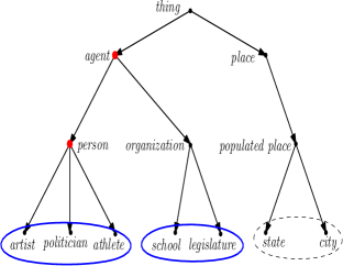
Figure 5: The concepts in red, agent and person, denote the design. The blue curves denote the partitions created after annotating the design and the dashed curved shows the free concepts of the selected design.

Example 3.3.

Again consider design $\{person,$ $agent\}$ over the taxonomy described in Figure 5. The free concepts of $\mathcal{S}$ are $\{state,$ $city\}$ as they are not in any partition of $\mathcal{S}$.

Let $DS$ be a data set in the domain of taxonomy $\mathcal{X}=$$(R,\mathcal{C},\mathcal{R})$ and $\mathcal{S}$ be a design over $\mathcal{X}$. $\mathcal{S}$ is the design of data set $DS$ iff for all concept $C\in\mathcal{S}$, all occurrences of concepts in the partition of $C$ are annotated by $C$. In this case, we say $DS$ is an instance of $\mathcal{S}$. For example, consider the design $\mathcal{T}=$ {person, organization} over the taxonomy in Figure 3. The data set in Figure 4 is an instance of $\mathcal{T}$ as all instances of concepts athlete, artist and politician, that belong to the partition of person, are annotated by person and all instances of concepts school and legislature, that constitute the partition of organization, are annotated by organization in the data set.

3.3 Design Queriability

Let $\mathcal{Q}$ be a set of queries over data set $DS$. Given design $\mathcal{S}$ over taxonomy $\mathcal{X}=$$(R,\mathcal{C},\mathcal{R})$, we would like to measure the degree by which $\mathcal{S}$ improves the effectiveness of answering queries in $\mathcal{Q}$ over $DS$. The value of this function should be larger for the designs that help the query interface to answer a larger number of queries in $\mathcal{Q}$ more effectively. As most entity-centric information needs are precision-oriented [5, 10], we use the standard metric of precision at $k$ ($p@k$ for short) to measure the effectiveness of answering queries over structured data sets [23]. The value of $p@k$ is the fraction of relevant answers in the top $k$ returned answers for the query. We average the values of $p@k$ over queries in $\mathcal{Q}$ to measure the amount of effectiveness in answering queries in $\mathcal{Q}$. The problem of design in order to maximize other objective functions, such as recall, is an interesting subject for future work.

Let $Q:(C,T)$ be a query in $\mathcal{Q}$ such that $C$ belongs to the partition of $P\in\mathcal{S}$. The query interface may consider only the documents that contain information about entities annotated by $P$ to answer $Q$. For instance, consider query $Q_{1}=$ $(politician,$ $JohnAdams)$ over data set fragment in Figure 4 whose design is {person, organization}. The query interface may examine only the entities annotated by person in this data set to answer $Q_{1}$. Thus, the query interface will avoid non-relevant results that otherwise may have been placed in the top $k$ answers for $Q$. It may further rank them according to its ranking function, such as the traditional TF-IDF scoring methods [23]. Our model is orthogonal to the method used to rank the candidate answers for the query.

The query interface still has to examine all documents that contain some mentions to the entities annotated by concept $P$ to answer $Q:(C,T)$. Nevertheless, only a fraction of these documents may contain information about entities of $C$. For instance, to answer query $(politician,JohnAdams)$ over the data set fragment in Figure 4, the query interface has to examine all documents that contain instances of concept person. Some documents in this set have matching entities form concepts other than politician, such as John Adams, the artist. We like to estimate the fraction of the results for $Q:(C,T)$ that contains a matching entity in concept $C$. Given all other conditions are the same, the larger this fraction is, the more likely it is that the query interface delivers more relevant answers, and therefore, a larger value of $p@k$ for $Q$.

Let $d_{DS}(C)$ denote the fraction of documents that contain entities of concept $C$ in data set $DS$. We call $d_{DS}(C)$ the frequency of $C$ over $DS$. When $DS$ is clear from the context, we denote the frequency of $C$ as $d(C)$. We want to compute the fraction of the returned answers for query $Q:(C,T)$ that contain a matching instance of concept $C$. These entities are annotated by concept $P$, such that $C$ is in the partition of $p$. Let $d(P)$ be the total frequency of leaf concepts in the partition of $P$. The fraction of these documents that contain information about $C$ is $\frac{d(C)}{d(P)}$. The larger this fraction is, the more likely it is that query interface returns more documents about entities of concept $C$ for query $Q:(C,T)$. Thus, it is more likely for query interface to return relevant answers for $Q$ and improve its $p@k$. For instance, assume that the mentions to the entities of concept artist appear more frequently in data set $DS$ than the ones of concept politician. Also assume that we only annotate person from $DS$. Given query $(politician,JohnAdams)$ it is more likely for articles about John Adams, the artist, to appear in the top-ranked answers than about John Adams, the politician.

We call the fraction of queries in $\mathcal{Q}$ whose concept is $C$ the popularity of $C$ in $\mathcal{Q}$. Let $u_{\mathcal{Q}}$ be the function that maps concept $C$ to its popularity in $\mathcal{Q}$. When $\mathcal{Q}$ is clear from the context, we simply use $u$ instead of $u_{\mathcal{Q}}$. The degree of improvement in value of $p@k$ in answering queries of concept $C$ over $DS$ is proportional to $\frac{u(C)\ d(C)}{d(p)}$. Hence, the amount of the contribution of queries of the concepts in partition of $P$ to the value of $p@k$ will be:

$$\sum_{C\in{\tt part}(P)}\frac{u(C)\ d(C)}{d(P)}.$$

Given all other conditions are the same, the larger this value is, the more likely it is that the query interface will achieve a larger $p@k$ value over queries in $\mathcal{Q}$.

Annotators, however, may make mistakes in identifying the correct concepts of entities in a collection [10]. An annotator may recognize some appearances of entities from concepts that are not $P$ as the occurrences of entities in $P$. For instance, the annotator of concept person may identify Lincoln, the movie, as a person. The accuracy of annotating concept $P$ over $DS$ is the number of correct annotations of $P$ divided by the number of all annotations of $P$ in $DS$. We denote the accuracy of annotating concept $P$ over $DS$ as ${\tt pr}_{DS}(P)$. When $DS$ is clear from the context, we show ${\tt pr}_{DS}(P)$ as ${\tt pr}(P)$. Hence, we refine our estimate to the following.

$$\sum_{C\in{\tt part}(P)}\frac{u(C)\ d(C)}{d(P)}\ {\tt pr}(P).$$ (1)

Next, we compute the amount of improvement that $\mathcal{S}$ provides for queries whose concepts do not belong to any partition, i.e., free concepts. If concept $C$ is a free concept with regard to design $\mathcal{S}$, the query interface has to examine all documents in the collection to answer $Q:(C,T)$. Thus, if $C$ is a free concept, the fraction of returned answers for $Q$ that contains a matching instance of concepts $C$ is $d(C)$. Using equation 1, we formally define the function that estimates the likelihood of improvement for the value of $p@k$ for all queries in a query workload over a data set annotated by design $\mathcal{S}$.

Definition 3.4.

The queriability of design $\mathcal{S}$ from taxonomy $\mathcal{X}$ over data set $DS$ is

$$QU(\mathcal{S})=\sum_{P\in\mathcal{S}}{\sum_{C\in{\tt part}(P)}\frac{u(C)\ d(C)\ {\tt pr}(P)}{d(P)}}\ +{\sum_{C\in{\tt free}(\mathcal{S})}u(C)d(C)}.$$ (2)

Similar to other optimization problems in data management, such as query optimization [16], the complete information about the parameters of the objective function, i.e. frequencies and popularities of concepts, may not be available at the design-time. Nevertheless, our empirical results in Section 7 indicate that one can effectively estimate these parameters using a small sample of the full data set. For instance, we show that the frequencies of concepts over a collection of more than a million documents can be effectively estimated using a sample of about three hundred documents.

3.4 Cost-Effective Design Problem

Given taxonomy $\mathcal{X}=$ $(\mathcal{C},\mathcal{R})$ and data set $DS$ in domain of $\mathcal{X}$, the function $w_{DS}:\mathcal{C}\rightarrow\mathbb{R}^{+}$, maps each concept $C$ to a real number that reflects the amount of resources used to annotate mentions of entities in $C$ from data set $DS$. When the data set is clear from the context, we simply denote the cost function as $w$. The enterprise may predict the costs of development and maintenance of annotation programs using available methods for predicting costs of software development and maintenance [7]. If the cost is running time, the enterprise may use current methods of estimating the execution time of concept annotators [20]. If there is not sufficient information to estimate the costs for concepts, the enterprise may assume that all concepts are equally costly. We will show in Sections 4, 5, and 6 that finding cost-effective designs is still challenging in the cases where concepts are equally costly.

Similar to previous works on cost-effective concept annotation [28], we assume that annotating certain concepts does not affect the cost and accuracies of other concepts. The reasons behind this assumption are two-fold. First, it usually takes significant amount of resources to develop, execute, and maintain a concept annotator even after pairing with other annotators. For instance, developers have to discover a large number of distinct features for each concept to accurately annotate them. Second, it may require exponential number of cost values to express the relationships between costs of concepts in a taxonomy, which is not realistic and makes the problem extremely complex to express. However, finding a simplified framework that can effectively express the problem with relationships between the costs of annotating different concepts is an interesting subject for future work.

The cost of annotating a data set under design $\mathcal{S}$ is the sum of the costs the concepts in $\mathcal{S}$. Budget $B$ is a positive real number that represents the amount of available resources for organizing the data set. Next, we formally define the problem of Cost-Effective Conceptual Design (CECD for short) as follows.

Problem 3.5.

Given taxonomy $\mathcal{X}$, data set $DS$ in the domain of $\mathcal{X}$, and budget $B$, we like to find design $\mathcal{S}$ over $\mathcal{X}$ such that $\sum_{C\in\mathcal{S}}w(C)\leq B$ and $\mathcal{S}$ delivers the maximum queriability over $\mathcal{X}$.

Unfortunately, the CECD problem cannot be solved in polynomial time in terms of input size unless $\mathbf{P}=\mathbf{NP}$.

Theorem 3.6.

The problem of CECD is $\mathbf{NP}$-hard.

Proof.

The problem of CECD can be reduced to the problem of choosing cost-effective concepts from a set of concepts by creating a taxonomy $\mathcal{X}=(R,\mathcal{C},\mathcal{R})$ where all nodes except for $R$ are leaf concepts, i.e. leaves. Since the problem of choosing cost-effective concepts from a set of concepts is $\mathbf{NP}$-hard [28], CECD will be $\mathbf{NP}$-hard. ∎

Because CECD is $\mathbf{NP}$-hard, we propose and study efficient approximation and pseudo-polynomial algorithms to solve it.

4 Level-Wise Algorithm

Level-wise algorithm solves the problem of CECD using a greedy approach. It returns a design whose concepts are all from a same level of the input taxonomy. Our algorithm finds the design with maximum queriability for each level using the algorithm proposed in [28], called approximate popularity maximization (APM for short), for finding the cost-effective subset of concepts over a set of concepts. It eventually delivers the design with largest queriability across all levels in the taxonomy.

Precisely, let $\mathcal{C}[i]$ be the set of all concepts of depth $i$ in $\mathcal{X}=$ $(R,\mathcal{C},\mathcal{R})$. For any concept $C\in\mathcal{C}[i]$, we define its popularity $u(C)$ to be the total popularity of its descendant leaf concepts in $\mathcal{X}$. Level-wise algorithm calls the APM algorithm to find the cost-effective subset of concepts for every $\mathcal{C}[i]$. It also computes the queriability of the design that contains only the most popular leaf concept, i.e., the leaf concept with maximum $u$ value. It then compares various selected designs across $\mathcal{C}[i]$s and returns the answer with maximum queriability as its solution for the problem of CECD over taxonomy $\mathcal{X}$. Figure 6 illustrates the level-wise algorithm. Let $|\mathcal{C}|$ denote the number of concepts in taxonomy $\mathcal{X}$. The APM algorithm runs in $O(|\mathcal{C}|\log|\mathcal{C}|)$. Thus, the time complexity of level-wise algorithm is $O(h|\mathcal{C}|\log|\mathcal{C}|)$ over taxonomy $\mathcal{X}$.

In addition to being efficient, level-wise algorithm also has bounded and reasonably small worst-case approximation ratio for an interesting case of CECD problem. Sometimes, it may be easier to use and manage designs whose concepts are not subclass/ superclass of each other. We call such a design a disjoint design. Our empirical results in Section 7 shows that this strategy returns effective designs in the cases that the budget is relatively small. In this case, we should restrict the feasible solutions in the CECD problem to be disjoint. We call this case of CECD, disjoint CECD.

Recent empirical results suggest that the distribution of concept frequencies over a large collection generally follows a power law distribution [31]. We show that the level-wise algorithm has a bounded and reasonably small worst-case approximation ratio for CECD with disjoint design given that distribution of concept frequencies follows a power law distribution. The following lemma bounds the queriability that is obtained from the free concepts in any solution given that distribution of concept frequencies follows a power law distribution.

Lemma 4.1.

Let $C_{\max}$ be the leaf concept in taxonomy $\mathcal{X}=(R,\mathcal{C},\mathcal{R})$ with maximum $u$ value and let assume that distribution of $u$ over leaf concepts follows a power law distribution. Let $\mathcal{S}$ be any schema. Then,

$$QU({\tt free}(\mathcal{S}))\leq 2u(\mathcal{C}_{\max})\log|\mathcal{C}|.$$

Proof.

We have:

$${\sum_{C\in{\tt free}(\mathcal{S})}u(C)d(C)\leq u(C_{\max})}\sum_{C\in{\tt free}(\mathcal{S})}d(C).$$

Since the frequencies of leaf concepts in $\mathcal{X}$ follow a “power law” distribution,

$$\sum_{C\in{\tt leaf}(\mathcal{C})}d(C)\leq 1+\log(|{\tt leaf}(\mathcal{C})|),$$

where ${\tt leaf}(\mathcal{C})$ is the set leaf concepts in $\mathcal{C}$ and $|{\tt leaf}(\mathcal{C})|$ is the number of such concepts. Since $|{\tt leaf}(\mathcal{C})|$ $\leq|\mathcal{C}|$,

$$QU({\tt free}(\mathcal{S}))\leq\sum_{C\in{\tt free}(\mathcal{S})}u(C)d(C)\leq(1+\log|\mathcal{C}|)\ u(C_{\max})\leq 2u(\mathcal{C}_{\max})\log|\mathcal{C}|.$$

∎

Level-wise    $\langle\!\langle$Input: $\left<\mathcal{X}\right>$$\rangle\!\rangle$ $\mathrm{sol}_{\tt level}\leftarrow 0$ and $\mathrm{sol}_{\tt max}\leftarrow 0$ $\langle\!\langle$Return the output of the best level$\rangle\!\rangle$ For $i=0$ to $h$ do For each concept $C$ in distance $i$ from the root $\mathcal{C}_{i}\leftarrow\mathcal{C}_{i}\cup C$ $\mathrm{sol}_{i}\leftarrow\text{ approximate solution over }(\mathcal{C}_{i})$ $\mathrm{sol}_{\tt level}\leftarrow\max(\mathrm{sol}_{\tt level},\mathrm{sol}_{i})$ $\langle\!\langle$Most Popular Leaf Concept Only$\rangle\!\rangle$ Let $C_{\max}$ be the leaf concept with the largest $u$ value. $\mathrm{sol}_{\tt max}\leftarrow u(C_{\max})+\sum_{C\in{\tt free}(C_{\max})}u(C)d(C)$ Return the best of $\mathrm{sol}_{\tt level}$ and $\mathrm{sol}_{\tt max}$

Figure 6: Level-wise algorithm.

Theorem 4.2.

Let $\mathcal{X}=(R,\mathcal{C},\mathcal{R})$ be a taxonomy with height $h$ and the minimum accuracy of ${\tt pr}_{\min}$ $=\min_{C\in\mathcal{C}}{{\tt pr}(C)}$. The Level-wise algorithm is a $O({h+\log|\mathcal{C}|\over{\tt pr}_{\min}})$-approximation for the CECD problem with disjoint solution on $\mathcal{X}$ and budget $B$ given that the distribution of frequencies in $\mathcal{C}$ follows a power law distribution.

Proof.

Let $\mathcal{S}^{*}$ be a disjoint schema over $\mathcal{X}$ with total cost at most $B$ that maximizes $QU$ function. Let $\mathcal{S}^{*}[i]$ be the set of concepts in $S^{*}$ of depth $i$. By the definition of disjointness, ${\tt part}(\mathcal{S}^{*}[i])$ $\cap$ ${\tt part}(\mathcal{S}^{*}[j])=\emptyset$, for all $1\leq i,j\leq h$. It follows:

$$QU(\mathcal{S}^{*})=\sum_{1\leq i\leq h}{QU(\mathcal{S}^{*}[i])}+QU({\tt free}(\mathcal{S}^{*})),$$

where $QU({\tt free}(\mathcal{S}^{*}))={\sum_{C\in{\tt free}(\mathcal{S}^{*})}u(C)d(C)}$ is the queriability obtained from the free concepts in $\mathcal{S}^{*}$.

We consider two possible cases. First, assume that $\sum_{i=1}^{h}$ $QU(\mathcal{S}^{*}[i])$ $\geq QU({\tt free}(\mathcal{S}^{*}))$. It immediately follows that the level-wise algorithm output gives a $(2h/{\tt pr}_{\min})$-approximation. In the other case in which $QU({\tt free}(\mathcal{S}^{*}))\geq$ $\sum_{1\leq i\leq h}QU(\mathcal{S}^{*}[i])$, by Lemma 4.1, extracting the concept with the maximum $u$ value gives a $(4\log(|\mathcal{C}|)/$ ${\tt pr}_{\min})$-approximation. These two cases together imply that we have an $O({h+\log|\mathcal{C}|\over{\tt pr}_{\min}})$-approximation. ∎

The value of ${\tt pr}_{\min}$ is generally large because concept annotation algorithm are reasonably accurate [9, 24].

5 Pseudo-polynomial Time Algorithm

In this section we describe a pseudo-polynomial time algorithm for the CECD problem over tree taxonomies. As many other optimization problems on the tree structure, one approach is to find an optimal solution bottom-up using dynamic programming technique. The main idea is to define the CECD problem over all subtrees of the given taxonomy $\mathcal{X}=(R,\mathcal{C},\mathcal{R})$. Next we show that in order to solve the subproblem defined over the subtree rooted at $C$, it is enough to solve the subproblems defined over the subtrees rooted at the children of $C$.

Let ${\tt child}(C)$ be the set of all children of the concept $C$ in $\mathcal{X}$. Moreover, let $\mathcal{X}_{C}$ be the subtree of $\mathcal{X}$ rooted at $C$. Formally given budget $B_{C}$, the subproblem over $\mathcal{X}_{C}$ is to find a design $\mathcal{S}_{C}\subseteq\mathcal{X}_{C}$ whose total cost is at most $B_{C}$ and the queriability of the partitions obtained by $\mathcal{S}_{C}$ is the maximum. Note that by annotating $\mathcal{S}_{C}$ in $\mathcal{X}_{C}$ there may exist a set of leaf concepts in $\mathcal{X}_{C}$ that do not belong to any of ${\tt part}(S)$ for $S\in\mathcal{S}$. Let ${\tt nullPart}(\mathcal{S}_{C},C)$ denotes the leaf concepts of $\mathcal{X}_{C}$ that are not assigned to any partition of $\mathcal{S}_{C}$.

In order to computer the maximum queriability of the best design in $\mathcal{X}_{C}$, one of the cases we should consider is the one in which $C$ is annotated. To apply dynamic programming in this case we need to evaluate the queriability of ${\tt part}(C)$ which is $\sum_{Ch\in{\tt child}(C)}\sum_{C^{\prime}\in{\tt nullPart}(\mathcal{S}_{Ch},Ch)}u(C^{\prime})d(C^{\prime})$. Thus besides the total queriability of partitions in $\mathcal{X}_{C}$, we should compute the value of $\sum_{C^{\prime}\in{\tt nullPart}(\mathcal{S}_{Ch},Ch)}u(C^{\prime})d(C^{\prime})$. All together we are required to solve the subproblem $Q$ defined over the subtree rooted at $C$ with parameter $B_{C}$ and $N_{C}$ where $B_{C}$ denotes the available budget for annotating concepts in $\mathcal{X}_{C}$ and $N_{C}$ denotes the value of $\sum_{C^{\prime}\in{\tt nullPart}(\mathcal{S}_{C},C)}u(C^{\prime})d(C^{\prime})$.

Further we assume that $u(C)$, $d(C)$, and $w(C)$ are positive integers for each $C\in\mathcal{C}$. In Section 7, we show that the algorithm can handle real values with scaling techniques in expense of reporting a near optimal solution instead of an optimal one. We define $D=\sum_{C\in{\tt leaf}(\mathcal{C})}d(C)$, $U=$ $\sum_{C\in{\tt leaf}(\mathcal{C})}u(C)$. Let $B_{\tt total}$ denote the total available budget. We propose an algorithm whose time complexity is polynomial in $U$, $D$, $B_{\tt total}$, and $|\mathcal{C}|$.

We have the following recursive rules for the non-leaf concepts in $\mathcal{C}$ based on the value of $Q$ for their children.

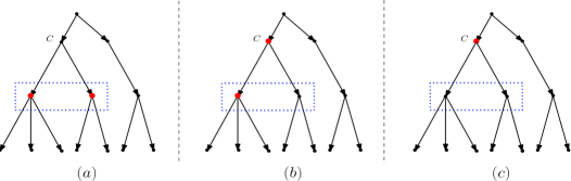
Figure 7: The concepts in red denote the ones that are picked in the design. $(a)$, $(b)$ and $(c)$ show three different types of the subproblems required to solve in order to compute $Q[C,B,0]$.

$$Q[C,B,0]=\max\{ \max_{\mathcal{B},\mathcal{N}}(\sum_{Ch\in{\tt child}(C)}Q[Ch,\mathcal{B}(Ch),\mathcal{N}(Ch)]+\frac{{\tt pr}(C)}{d(C)}{\sum_{Ch\in{\tt child}(C)}\mathcal{N}(Ch)}),$$

$$\max_{\mathcal{B}^{\prime}}\sum_{Ch\in{\tt child}(C)}Q[Ch,\mathcal{B}^{\prime}(Ch),0]\}$$

For each $Ch$, $\mathcal{B}(Ch)$, $\mathcal{B}^{\prime}(Ch)$ and $\mathcal{N}(Ch)$ are integer values satisfying the following conditions: (1) $B=w(C)+\sum_{Ch\in{\tt child}(C)}\mathcal{B}(Ch)$, (2) $B=\sum_{Ch\in{\tt child}(C)}\mathcal{B}^{\prime}(Ch)$, and (3) $UD\geq\sum_{Ch\in{\tt child}(C)}\mathcal{N}(Ch)$.

The first term in the recursive rule corresponds to the case in which we select concept $C$ in the output design ($(b)$ and $(c)$ in Figure 7) and the second term corresponds to the case in which for any child of $C$, $Ch$, ${\tt nullPart}(Ch)=\emptyset$ ($(a)$ in Figure 7). In a design $\mathcal{S}_{C}$ in $\mathcal{X}_{C}$ with the maximum queriability and empty ${\tt nullPart}$ whose total cost is $B$, either $C$ is selected in the design and the budget $B-w(C)$ is divided among the children of $C$ (first term of the above rule), or the whole budget $B$ is divided among the children of $C$ and all leaf concepts of $\mathcal{X}_{C}$ is assigned to a proper descendant of $C$ in the design (second term of the above rule).

Similarly, for the case in which $N\neq 0$ we have the following recursive rule:

$$Q[C,B,N] =\max_{\mathcal{B},\mathcal{N}}\sum_{Ch\in{\tt child}(C)}Q[Ch,\mathcal{B}(Ch),\mathcal{N}(Ch)]$$

where $\mathcal{B}=\{{\mathcal{B}(Ch)|Ch\in{\tt child}(C)}\}$ and $\mathcal{N}=$ $\{\mathcal{N}(Ch)|$ $Ch\in{\tt child}(C)\}$ such that $B=\sum_{Ch\in{\tt child}(C)}\mathcal{B}(Ch)$ and $N=\sum_{Ch\in{\tt child}(C)}\mathcal{N}(Ch)$. For each leaf concept $C_{\ell}$ in $\mathcal{C}$, we have the following.

• $Q[C_{\ell},B,N]=0\text{ if }N=u(C_{\ell})d(C_{\ell})\text{ and }-\infty\text{ otherwise }$

• $Q[C_{\ell},B,0]={\tt pr}(C_{\ell})u(C_{\ell})\text{ if }B\geq w(C_{\ell})\text{ and }-\infty\text{ otherwise}.$

The maximum value of the queriability on $\mathcal{X}=(R,\mathcal{C},\mathcal{R})$ is

$$\max_{N}Q[R,B_{\tt total},N]+N,$$ (3)

where $B_{\tt total}$ is the total available budget. The first term, $Q[R,B_{\tt total},N]$, denotes the profit obtained form the partitions of an optimal design and the second term corresponds to the profit obtained from the free concepts with respect to the output design.

To compute the running time of the algorithm we need to give an upper bound on the number of cells in $Q$ and the time required to compute the value of each cell. The time to compute a single cell in $Q$ is exponential in terms of the maximum degree of the taxonomy. Consequently, the algorithm runs much faster if the maximum degree in $\mathcal{X}$ is bounded by a small constant. As we show next, we can modify the taxonomy $\mathcal{X}$ to obtain taxonomy $\mathcal{X}^{\prime}$ such that each concept $C$ in $\mathcal{X}^{\prime}$ has at most two children and the number of nodes in $\mathcal{X}^{\prime}$ is at most twice the number of nodes in $\mathcal{X}$. Since each node in $\mathcal{X}^{\prime}$ has two children, the required amount of time to compute a single cell in $Q$ is $O(B_{\tt total}UD)$; at most $B_{\tt total}$ ways to divide the budget between the two children and at most $UD$ ways to divide $N$ between the two children. Since the first argument in $Q$ can be any of the concepts in $\mathcal{C}$, $N\leq UD$ and $B\leq B_{\tt total}$, there are $O(B_{\tt total}UD)$ cells to evaluate in order to compute the design with maximum queribility. Thus the total time for computing all cells in $Q$ is $O(|\mathcal{C}|(B_{\tt total}UD)^{2})$.

Next, we explain how to transform an arbitrary taxonomy to a binary taxonomy. Let $C$ be a non-leaf concept in $\mathcal{X}$. We replace the induced subtree of $C\cup{\tt child}(C)$ with a full binary tree $\mathcal{X}_{C}^{\prime}$ whose root is $C$ and whose leaves are ${\tt child}(C)$ as shown in Figure 8. Some internal nodes of $\mathcal{X}_{C}^{\prime}$ do not correspond to any node in $\mathcal{X}$. We refer to such internal nodes as dummy nodes, and set their cost to $B_{\tt total}+1$ to make sure that our algorithm does not include them in the output design.

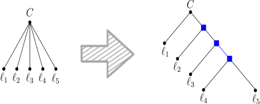
Figure 8: Transforming an input taxonomy $\mathcal{X}$ into a binary taxonomy. Blue square nodes correspond to dummy nodes.

Applying the mentioned transformation to all nodes of $\mathcal{X}$, we obtain a binary taxonomy $\mathcal{X}^{\prime}=(R,\mathcal{C}^{\prime},\mathcal{R}^{\prime})$. The number of nodes in $\mathcal{C}^{\prime}$ is at most twice the number of nodes in $\mathcal{C}$. It follows that the running time of our pseudo-polynomial algorithm on the input $\mathcal{X}^{\prime}$ is $O(|\mathcal{C}|(B_{\tt total}UD)^{2})$.

Since this transformation does not change the subset of leaf concepts in the subtree rooted in any internal node, any internal node in $\mathcal{X}$ corresponds to a solution in $\mathcal{X}^{\prime}$ with the same cost and queriability. Since dummy nodes are too expensive to be chosen, they do not introduce any new solution to the set of feasible solutions.

Theorem 5.1.

There is an algorithm to solve the CECD problem over taxonomy $\mathcal{X}=(R,\mathcal{C},\mathcal{R})$ with budget $B$ in $O(|\mathcal{C}|B^{2}U^{2}D^{2})$.

Table 1 presents a summary of proposed algorithms for the CECD problem.

Algorithm	Approximation ratio	Running time
Level-wise	$O((h+\log|\mathcal{C}|)/{\tt pr}_{\min})$ (Disjoint CECD)	$O(h|\mathcal{C}|\log(|\mathcal{C}|))$
Dynamic Programming	Pseudo-polynomial	$O(|\mathcal{C}|B^{2}U^{2}D^{2})$

Table 1: Algorithms for the CECD problem.

6 Cost-Effective Design for DAG Taxonomies

6.1 Directed Acyclic Graph Taxonomies

While taxonomies are traditionally in form of trees, many of them have evolved into directed acyclic graphs (DAGs) to model more involved subclass/ superclass relationships between concepts in their domains. Figure 9 shows fragments of schema.org taxonomy. Some concepts in this taxonomy are included in multiple superclasses. For example, a hospital is both a place and an organization. Therefore, a tree structure is not able to represent these relationships.

Formally, a directed acyclic graph taxonomy $\mathcal{X}=$ $(R,\mathcal{C},\mathcal{R})$, (DAG taxonomy for short), is a DAG, with vertex set $\mathcal{C}$, edge set $\mathcal{R}$, and root $R$. $\mathcal{C}$ is a set of concepts, $(D,C)\in\mathcal{R}$ iff $D,C\in\mathcal{C}$ and $D$ is a superclass of $C$. Finally, $R$ is a node in $\mathcal{X}$ without any superclass. A concept $C\in\mathcal{C}$ is a leaf concept iff it has no subclass in $\mathcal{X}$; i.e, there is not any node $D\in\mathcal{C}$ where $(C,D)\in\mathcal{R}$. The definitions of child, ancestor, and descendant over tree taxonomies naturally extends to DAG taxonomies.

Figure 9: Fragments of schema.org taxonomy

6.2 Design Queriability

Design $\mathcal{S}$ over DAG taxonomy $\mathcal{X}=$ $(R,\mathcal{C},\mathcal{R})$ is a non-empty subset of $\mathcal{C}-\{{R}\}$. Due to the richer structure of DAG taxonomies, designs over DAG taxonomies may improve the effectiveness of answering queries in more ways than the ones over tree taxonomies. For example, let data set $DS$ be in the domain of the DAG taxonomy in Figure 9, and $\mathcal{S}_{1}=$ $\{place,$ $organization\}$ be a design. The query interface will examine the documents that are organized under organization in $DS$ to answer queries about concept airline. As query interface does not have sufficient information to pinpoint the entities of concept airline in $DS$, it may return some non-relevant answers for these queries, e.g., matching entities that are NGOs. On the other hand, because concept hospital is a subclass of both place and organization, its entities in $DS$ are annotated by both concepts place and organization. By examining the entities that are annotated by both place and organization, the query interface is able to identify the instances of hospital in $DS$. Thus, it will not return entities that belong to other concepts when answering queries about instances of hospital. Generally, the query interface may pinpoint instances of some concepts in the data set by considering the intersections of multiple concepts in a design over a DAG taxonomy. Hence, subsets of a design may create partitions in a DAG taxonomy. Next, we extend the notion of partitions for designs over DAG taxonomies.

Definition 6.1.

Let $\mathcal{S}$ be a design over DAG taxonomy $\mathcal{X}=(R,\mathcal{C},\mathcal{R})$, and let $C\in\mathcal{C}$ be a leaf concept. An ancestor $A$ of $C$ in $\mathcal{S}$ is $C$’s direct ancestor iff one of the following properties hold.

• $A=C$.

• For each $D\in\mathcal{S}$, if $D$ is an ancestor of $C$ then $D$ is not a descendant of $A$.

The full-ancestor-set of $C$ is the set of all its direct ancestors. For instance, the set $\{place,$ $organization\}$ is the full-ancestor-set of the concept hospital in design $\mathcal{S}_{1}=$ $\{place,$ $organization\}$, and the set $\{place,$ $local\leavevmode\nobreak\ business\}$ is the full-ancestor-set of the concept hospital in design $\mathcal{S}_{2}=$ {place, organization, local business} over the taxonomy in Figure 9.

Definition 6.2.

Given design $\mathcal{S}$ over DAG taxonomy $\mathcal{X}=$ $(R,\mathcal{C},\mathcal{R})$, the partition of a set of concepts $\mathcal{D}\subseteq\mathcal{S}$ is a set of leaf concepts $\mathcal{L}\subseteq\mathcal{C}$ such that for every leaf concept $L\in\mathcal{L}$, $\mathcal{D}$ is the full-ancestor-set of $L$.

For instance, hospital belongs to the partition of $\{place,$
$organization\}$ in $\mathcal{S}_{1}$. But, it does not belong to the partition of $\{{place}\}$, since $\{{place}\}$ is not the full-ancestor-set of hospital. The definitions of functions ${\tt part}$ and ${\tt free}$ over DAG taxonomies extend from their definitions over tree taxonomies.

Similar to tree taxonomies, we define the frequency of partition $P$, denoted by $d(P)$, as the frequency of the intersection of concepts in its root. Using a similar analysis to the one in Section 3.3, we define the queriability of conceptual design $S$ over DAG taxonomy $\mathcal{X}=$ $(R,\mathcal{C},\mathcal{R})$ as follows.

$$QU(\mathcal{S})=\sum_{P\in{\tt all-parts}(\mathcal{S})}{\sum_{C\in P}u(C)d(C)\over d(P)}+{\sum_{C\in{\tt free}(\mathcal{S})}u(C)d(C)}.$$ (4)

The function ${\tt all-parts}(\mathcal{S})\subseteq 2^{\mathcal{S}}$ returns the collection of all full-ancestor-sets of $\mathcal{S}$ in $\mathcal{X}$. We remark that the size of ${\tt all-parts}(\mathcal{S})$ is linear, since we have at most one new partition per any leaf concept in $\mathcal{X}$.

6.3 Hardness of Cost-Effective Design Over DAG Taxonomies

We define the CECD problem over DAG taxonomies similar to the CECD problem over tree taxonomies. Following from the $\mathbf{NP}$-hardness results for CECD problem over tree taxonomy, CECD problem over DAG taxonomies is NP-hard. In this section, we prove that finding an approximation algorithm with a reasonably small bound on its approximation ratio for the problem CECD over DAG taxonomies is significantly hard. Unfortunately, this is true even for the special cases where concepts in the taxonomy have equal costs or the design is disjoint.

We show that the CECD problem over a DAG taxonomy generalizes a hard problem in the approximation algorithms literature: Densest-$k$-Subgraph [22]. Given a graph $G=(V,E)$, in the the Densest-$k$-Subgraph problem, the goal is to compute a subset $U\in V$ of size $k$ that maximizes the number of edges in the induced subgraph of $U$. It is known that, unless $\mathbf{P}=\mathbf{NP}$, no polynomial time approximation scheme, i.e., PTAS, exists to compute the densest subgraph [22]. Moreover, there are strong evidences that Densest-$k$-Subgraph does not admit any approximation guarantee better than polylogarithmic factor [6, 2]. The following theorem shows that approximating the $k$-densest subgraph reduces to approximating CECD.

Lemma 6.3.

Let $\mathcal{S}$ be a design over taxonomy $\mathcal{X}=(R,\mathcal{C},\mathcal{R})$ that is constructed from input $G=(V,E)$ as above. Let $S_{v}\in\mathcal{C}\setminus\mathcal{S}$ be a non-leaf concept. Then $QU(\mathcal{S}\cup\{{S_{v}}\})\geq QU(\mathcal{S})$.

Proof.

After annotating a non-leaf concept $S_{v}$, each leaf concept $C$ will be contained by a partition of either smaller or the same size. Since the contribution of a leaf concept $C$ to $QU$ only depends on the size of the partition contains $C$ and this dependence is a non-decreasing function in terms of the size of partition, after annotating $S_{v}$ the contribution of $C$ to $QU$ either increases or remains unchanged. Thus $QU(\mathcal{S}\cup\{{S_{v}}\})\geq QU(\mathcal{S})$. ∎

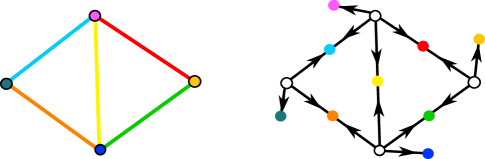
Figure 10: Reducing the Densest-$k$-Subgraph problem to CECD over DAG taxonomies where colors show correspondences in the reduction. The input graph for densest $k$-subgraph problem is shown on the left and its corresponding DAG taxonomies are in right. Colored vertices are leaf concepts and white vertices are non-leaf concepts in the DAG taxonomy.

The main result of this section is the following theorem.

Theorem 6.4.

A $(\log m)$-approximation algorithm for the CECD problem over DAG taxonomy with $m$ number of concepts implies that there is an algorithm for the Densest-$k$-Subgraph problem on $G=(V,E)$ with $n$ vertices that returns a $O(\log n)$-approximate solution.

Proof.

Given $G$ and $k$, we build an instance of the CECD over a DAG taxonomy as follows. For each edge $e\in E$, we introduce a leaf concept $a_{e}$ and an for each vertex $v\in V$, we introduce a leaf concept $a_{v}$ and a non-leaf concept $S_{v}$ such that $S_{v}$ is the super class of $a_{v}$ and all the concepts corresponding to the incident edges to $v$ in $G$. Further, we set the budget $B$ to $k$, the cost of each non-leaf concept to $1$, and the cost of each leaf concept to $k+1$.

Note that if we select $S_{v}$ and $S_{u}$ in the design and $(u,v)\in E$, then $a_{e}$ will be a singleton partition. We also set the popularities and frequencies of all concepts in the taxonomy respectively to the same fixed values $u$ and $d$. Let $m$ be the number of edges in $G$ (or equivalently the number of leaf concepts in $\mathcal{C}$) and $n$ be the number of vertices in $G$ (or equivalently the number of non-leaf concepts in $\mathcal{C}$). For each partition $p\in{\tt part}(\mathcal{S})$ we set $d(p)=1/(m\log n)$ if $|p|=1$ and $d(p)=1$ otherwise.

By Lemma 6.3, annotating a non-leaf concept will not decrease the queribility of the design. Since the leaf concepts are not affordable, and annotating a non-leaf concept will not decrease the total queribility, there exists an optimal design that annotates exactly $k$ non-leaf concepts. Note that in any design $\mathcal{S}$ of size $k$, the contribution of any leaf concept in a non-singleton partition (partition of size greater than one) is exactly $u\cdot d$. In what follows we show that a $\log n$-approximation algorithm for the CECD problem implies a $O(\log n)$-approximation for the Densest-$k$-Subgraph problem. To this end, by contradiction, let $\mathcal{A}$ be a $\log n$-approximation algorithm of CECD problem.

Let $H_{\mathcal{S}}$ be the set of vertices in $G$ of whose corresponding non-leaf concepts in $\mathcal{C}$ are annotated in design $\mathcal{S}$. $E(H_{\mathcal{S}})$ denotes the set of edges with both endpoint in $H$ which corresponds to the set of edge-concepts of $\mathcal{C}$ whose both non-leaf concepts corresponding to their endpoints are annotated by $\mathcal{S}$.

Let $\mathcal{S}_{\textsc{OPT}}$ be an optimal solution of the CECD problem. Suppose that $QU(\mathcal{S}_{\textsc{OPT}})=(t+r)\cdot m\log n+(m-t+n-r)$ where $t$ denotes the number of edges in $H_{\mathcal{S}_{\textsc{OPT}}}$ and $r$ denotes the number of vertices in $H_{\mathcal{S}_{\textsc{OPT}}}$ whose all incident edges are in $E(H_{\mathcal{S}_{\textsc{OPT}}})$. It is straightforward to see that the corresponding leaf concepts to edges in $E(H_{\mathcal{S}_{\textsc{OPT}}})$ and vertices with all incident edges in $E(H_{\mathcal{S}_{\textsc{OPT}}})$ are the only singleton partitions with respect to design $\mathcal{S}_{\textsc{OPT}}$.

Now, let $\mathcal{S}_{\mathcal{A}}$ be the design returned by $\mathcal{A}$ and similarly assume that $QU(\mathcal{S}_{\mathcal{A}})=(t^{\prime}+r^{\prime})\cdot m\log n+(m-t^{\prime}+n-r^{\prime})$. Since $\mathcal{A}$ is a $\log n$-approximation algorithm of the CECD problem, $(t+r)\cdot m\log n+(m-t+n-r)$ is at most $\log n\cdot((t^{\prime}+r^{\prime})\cdot m\log n+(m-t^{\prime}+n-r^{\prime}))$. Thus,

$$t(m\log n-1)\leq t^{\prime}(m\log^{2}n-1)+r^{\prime}m\log^{2}n+(m+n)\log n.$$

Note that since the size of a feasible design is $k$, $r^{\prime}\leq k$. Thus with some simplifications,

$${tm\log n\over 2}\leq t^{\prime}(m\log^{2}n)+km\log^{2}n+2m\log n,$$

which implies that

$$t\leq 2t^{\prime}\log n+2k\log n+4\leq 5\log n\cdot\max\{{k,t^{\prime}}\}.$$ (5)

Now consider the greedy approach of Densest-$k$-Subgraph problem such that in each step the algorithm picks a vertex $v$ and add it to the already selected set of vertices $S$ if $v$ has the maximum number of edges incident to $S$. It is easy to see that the greedy approach guarantee $k/2$ number of edges. Note that if the input graph has less than $k/2$ edges, we can solve Densest-$k$-Subgraph problem optimally by picking all edges. Using the simple greedy approach and the result returned by $\mathcal{A}$, we can find a set of $k$ vertices whose induced subgraph has at least $\max\{{k/2,t^{\prime}}\}$ number of edges. Thus by (5), we can find a $O(\log n)$-approximate solution of the Densest-$k$-Subgraph problem which completes the proof. ∎

Since the concepts in the instance of the CECD problem discussed in the proof of Theorem 6.4 have equal costs and its optimal solution is disjoint, i.e., there is no directed path between any two of concepts in the design, the hardness results of Theorem 6.4 is true even for the special cases of CECD problem over DAG taxonomies where the concepts are equally costly and/or the problem has disjoint solutions.

Figure 11 illustrates a simple example for which the level-wise algorithm is arbitrarily worse than the optimal solution over DAG taxonomies. For the sake of simplicity, let $d$ and $u$ values be positive integers. Let $u(C_{4})=4$, $d(C_{4})=1$, $u(C_{5})=1$, $d(C_{5})=M$, $u(C_{6})=M$, $d(C_{6})=1$, $u(C_{7})=1$ and $d(C_{7})=M$. Also, let $w(C_{1})=w(C_{2})=w(C_{3})=1$, and $B=2$. The greedy algorithm first picks $C_{1}$ because of its high immediate queriability, and then $C_{2}$ or $C_{3}$ (but not both of them). So its total queriability is $5$. On the other hand, by picking $C_{2}$ and $C_{3}$ one may acquire $C_{6}$ for free, whose queriability is $M$. Since we can choose $M$ to be any number, the optimal solution can be arbitrarily better that the solution delivered by the greedy approach. Intuitively, the situation can be exacerbated to a large extent if the subset with large queriability can be obtained by intersecting more than two concepts.

Figure 11: An instance of CECD problem over DAG taxonomy

7 Experiments

7.1 Experiment Setting

Table 2: The sizes and heights of taxonomies and the sizes of corresponding datasets and query workloads.

Taxonomy	T1	T2	T3	T4	T5	T6	T7	T8
#Concept	10	17	17	28	63	185	279	2269
#Height	2	2	3	7	6	8	8	9
#Documents	68982	267653	88479	1470661	1470661	1470661	1470661	1470661
#queries	648	256	146	4219	4888	4728	5216	11156

7.1.1 Taxonomies and datasets

Taxonomies: We have extracted eight taxonomies from YAGO ontology version 2008-w40-2 [15] to validate our model and evaluate effectiveness and efficiency of our proposed algorithms. YAGO organizes its concepts using subclass relationships in a DAG with a single root. We have created the breath-first tree of YAGO and randomly selected the concepts from the tree for our taxonomies. To validate our model, we have to compute and compare the effectiveness of answering queries using every feasible design over a taxonomy. Thus, we need tree taxonomies with relatively small number of concepts for our validation experiments. We have extracted three tree taxonomies with relatively small numbers of nodes, called T1, T2 and T3, to use in our validation experiments. The selected concepts for T1, T2 and T3 are from level 3 to 6 of the full YAGO tree which has a total of 9 levels. We have further picked five other tree taxonomies with larger numbers of concepts, denoted as T4, T5, T6, T7 and T8. The concepts for T4 and T5 are selected from level 3 to 6 of the full YAGO tree. The concepts for T6 and T7 are randomly selected from levels 2 to 9 of the full YAGO tree. T8 contains all concepts from the original YAGO tree that appear at least once in the collection of English Wikipedia articles. We use all tree taxonomies to evaluate the effectiveness and efficiency of our proposed algorithms. Table 2 shows the properties of these taxonomies.

Datasets: We have used the collection of English Wikipedia articles from the Wikipedia dump of October 8, 2008 that is annotated by concepts from YAGO ontology in our experiments [15]. This collection originally contains 2,666,190 articles of which 1,470,661 articles are annotated by at least a concept from YAGO ontology. For each taxonomy in our set of taxonomies, we have extracted a subset of the original Wikipedia collection where each document contains at least a mention to an entity of a concept in the taxonomy. We use each dataset in the experiments over its corresponding taxonomy. Table 2 shows the properties of these eight datasets. The annotation accuracies of the concepts in selected taxonomies over these datasets are between 0.8 and 0.95.

7.1.2 Query Workload

We use a subset of Bing, query log whose relevant answers are Wikipedia articles [14]. The relevant answers for each query in this query workload have been determined using the click-through information by eliminating noisy clicks. Each query contains between one to six keywords and has between one to two relevant answers with most queries having one relevant answer. Because the query log does not have the concepts behind its queries, we adapt an automatic approach to find the leaf concept from the taxonomy associated with each query. We label each query by the concept of the matching instance in its relevant answer(s). Then, we select queries labeled with a single concept. Using this method, we create a query workload per each of our datasets. It is well known that the effectiveness of answering some queries may not be improved by annotating the dataset [26]. For instance, all candidate answers for a query may contain mentions to the entities of the query concept. To reasonably evaluate our algorithms, we have ignored the queries whose rankings remain the same over the unannotated version and the version of the dataset where all concepts in the taxonomy are annotated. Table 2 shows the information about our query workloads.

We estimate the popularities of concepts for each taxonomy by sampling a small subset of randomly selected queries from their corresponding query workloads. We compute the popularity of each concept using estimation error rate of 5% under the 95% confidence level. The number of sampled queries are between 100 and 500 for each taxonomy. Because some concepts in a taxonomy may not appear in its query workload, we smooth the popularity of a concept $C$, $u(C)$, using the Bayesian $m$-estimate method [23]: $\hat{u}(C)=\frac{\hat{P}(C|QW)+mp}{m+\sum_{C}{\hat{P}(C|QW)}}$, where $\hat{P}(C|QW)$ is the probability that $C$ occurs in the query workload $QW$ and $p$ denotes the prior probability. We set the value of the smoothing parameter, $m$, to 1 and use a uniform distribution for all the prior probabilities.

7.1.3 Query Interface

We index our datasets using Lucene. Given a query, we rank its candidate answers using BM25 ranking formula, which is shown to be more effective than other similar document ranking methods [23]. Then, we apply the information about the concepts in the query and documents to return the answers whose matching instances have the same concept as the concept of the query. If the concept in the query has not been annotated in the collection, the query interface returns the list of documents ranked by BM25 method without any modification. We have implemented our query interface and algorithms in Java 1.7 and performed our experiments on a Linux server with 100 GB of main memory and two quad core processors.

7.1.4 Effectiveness Metric

Because all queries in our query workloads have one or two relevant answers, we measure the ranking quality of answering queries over a dataset using mean reciprocal rank (MRR) [23]. MRR is an inverse of the rank of the first relevant answer in the returned list of answers. MRR is used to measure the effectiveness of results for queries that have a small number of relevant answers [23]. Since most queries in our query workload have a single relevant answer, MRR is an appropriate metric to measure the effectiveness of their results.

We also report the precision at top 3 answers ($p@3$) for our results. Because all queries in our query workloads have one or two relevant answers, we measure the ranking quality of answering queries over a dataset using precision at top 3 answers ($p@3$) [23]. One may also use a larger number of top answers to measure the precision and ranking quality of the results. However, since the total numbers of relevant answers in our query workloads are less than three, the maximum possible value for $p@k$ is at most $\frac{2}{k}$. Consequently, the reported values will be very small when $k$ is large. Thus, using larger values of $k$ makes comparing and analyzing the effectiveness of query results rather hard. Further, using larger values of $k$ may hide the advantages of some query interfaces. For instance, let a query have one relevant answer. Assume that the query interface $I1$ places the relevant answer to the query in the first position and the query interface $I2$ places it in the 10th position of their returned results. Intuitively, the result of $I1$ is more effective than $I2$. The values of $p@3$ are $0.33$ for $I1$ and $0$ for $I2$; however, the values of $p@10$ for both of them will be equal.

We measure the statistical significance of our results using the paired-$t$-test at a significant level of 0.05.

7.1.5 Cost Models

We use three models for generating costs of concept annotation. First, we assign a randomly generated cost to each concept in a taxonomy. The results reported for this model are averaged over 5 sets of random cost assignments per budget. We call this model random cost model. Second, when there is not any reliable estimation available for the cost of annotating concepts, an organization may assume that all concepts are equally costly. Hence, in our second cost model, we assume that all concepts in the input taxonomy have equal cost. We name this model uniform cost model. These two cost models have also been used to model the costs of large-scale data curation [13, 28, Rekatsinas:2014:CSF:2588555.2610504]. Lastly, an organization may also assume that the cost of a concept depends on how likely the concept appears in a collection. Hence, in our third cost model, we assume that a cost of a concept is proportional to its frequency. We call this model frequency-based cost model. We use a range of budgets between 0 and 1 with a step size of 0.1 where 1 means sufficient budget to annotate all leaf concepts in a taxonomy and 0 means no budget is available.

7.2 Validating Queriability Function

Oracle: Given a fixed budget, Oracle enumerates all feasible designs over the input taxonomy. Given an effectiveness metric, such as MRR, for each design, it computes the average the effectiveness metric for all queries in the query workload over the dataset annotated by the design. It then returns the design with maximum value of the average effectiveness metric.

Popularity Maximization (PM): Following the traditional approach towards conceptual design for databases, one may select concepts in a design that are more important for users [16]. Hence, we implement an algorithm, called PM, that enumerates all feasible designs, such as $\mathcal{S}$, in a taxonomy and returns the one with the maximum value of $\sum_{p\in{\tt part}(\mathcal{S})}\sum_{C\in p}$ $u(C){\tt pr}(p)$. This design contains the concepts that are more frequently queried by users and also annotated more accurately.

Queriability Maximization (QM): QM enumerates all feasible designs over the input taxonomy and returns the one with the maximum queriability as computed in Section 3.3.

Because we would like to explore how accurately PM and QM predict the amount of improvement in the effectiveness of answering queries by a design, we assume that these algorithms have complete information about the popularities and frequencies of concepts. Since Oracle, PM and QM algorithms enumerate all feasible designs, it is not possible to run them over large taxonomies. Hence, we run these algorithms over small taxonomies, i.e. T1, T2 and T3.

Table 4 illustrates the average MRR achieved by Oracle, QM and PM over taxonomies T1, T2 and T3 for various budgets. We do not report the values of average MRR for budgets greater than 0.7 for T1 and T2 and 0.6 for T3 because all algorithms are equally effective. The values of MRR show at budget 0.0 is the one achieved by BM25 ranking without annotating any concept in the datasets. We note that there is no improvement in average MRR over taxonomy T1 for budget 0.1 under uniform cost because each concept in the taxonomy costs more than 0.1.

Table 3: Average $p@3$ for Oracle, PM and QM over T1, T2 and T3. Statistically significant differences between PM and QM and between Oracle and QM are marked in bold and italic, respectively. $B$ denotes a given budget.

		Uniform Cost			Random Cost			Frequency-based Cost
	$B$	Oracle	QM	PM	Oracle	QM	PM	Oracle	QM	PM
T1	0.0	0.089
	0.1	0.089	0.089	0.089	0.115	0.115	0.107	0.180	0.180	0.180
	0.2	0.149	0.149	0.089	0.159	0.159	0.102	0.180	0.180	0.180
	0.3	0.168	0.168	0.091	0.170	0.170	0.094	0.180	0.180	0.180
	0.4	0.183	0.177	0.106	0.183	0.177	0.116	0.180	0.180	0.180
	0.5	0.192	0.192	0.166	0.192	0.192	0.146	0.180	0.180	0.180
	0.6	0.194	0.193	0.185	0.194	0.193	0.177	0.180	0.180	0.180
	0.7	0.195	0.195	0.194	0.195	0.194	0.190	0.180	0.180	0.180
T2	0.0	0.200
	0.1	0.241	0.232	0.234	0.252	0.234	0.233	0.254	0.249	0.249
	0.2	0.275	0.272	0.245	0.283	0.276	0.246	0.292	0.289	0.289
	0.3	0.303	0.285	0.247	0.309	0.298	0.248	0.303	0.293	0.293
	0.4	0.318	0.315	0.250	0.318	0.316	0.264	0.322	0.322	0.322
	0.5	0.320	0.318	0.258	0.322	0.319	0.278	0.323	0.322	0.322
	0.6	0.323	0.322	0.290	0.323	0.321	0.299	0.323	0.323	0.323
	0.7	0.326	0.324	0.326	0.326	0.323	0.314	0.323	0.323	0.323
T3	0.0	0.171
	0.1	0.222	0.210	0.208	0.240	0.235	0.235	0.210	0.210	0.210
	0.2	0.260	0.249	0.258	0.271	0.265	0.258	0.231	0.231	0.231
	0.3	0.281	0.269	0.258	0.292	0.289	0.278	0.265	0.249	0.249
	0.4	0.304	0.304	0.288	0.304	0.304	0.293	0.288	0.288	0.288
	0.5	0.306	0.304	0.299	0.306	0.304	0.303	0.304	0.304	0.304
	0.6	0.306	0.306	0.306	0.306	0.306	0.306	0.304	0.304	0.304

Table 4: Average MRR for Oracle, PM and QM over T1, T2 and T3. Statistically significant differences between PM and QM and between Oracle and QM are marked in bold and italic, respectively. $B$ denotes a given budget.

		Uniform Cost			Random Cost			Frequency-based Cost
	$B$	Oracle	QM	PM	Oracle	QM	PM	Oracle	QM	PM
T1	0.0	0.187
	0.1	0.187	0.187	0.187	0.259	0.255	0.239	0.475	0.475	0.475
	0.2	0.362	0.362	0.197	0.385	0.384	0.226	0.475	0.475	0.475
	0.3	0.415	0.406	0.203	0.424	0.417	0.212	0.475	0.475	0.475
	0.4	0.459	0.459	0.227	0.461	0.461	0.262	0.475	0.475	0.475
	0.5	0.492	0.492	0.400	0.492	0.492	0.341	0.475	0.475	0.475
	0.6	0.501	0.501	0.444	0.501	0.499	0.426	0.475	0.475	0.475
	0.7	0.507	0.507	0.497	0.507	0.504	0.476	0.475	0.475	0.475
T2	0.0	0.342
	0.1	0.504	0.479	0.504	0.515	0.471	0.482	0.598	0.598	0.598
	0.2	0.577	0.543	0.551	0.616	0.586	0.559	0.662	0.662	0.662
	0.3	0.641	0.629	0.574	0.677	0.661	0.576	0.677	0.674	0.674
	0.4	0.729	0.729	0.586	0.725	0.725	0.616	0.741	0.741	0.741
	0.5	0.745	0.745	0.615	0.744	0.742	0.652	0.747	0.747	0.747
	0.6	0.751	0.751	0.647	0.754	0.754	0.695	0.748	0.748	0.748
	0.7	0.763	0.763	0.759	0.763	0.758	0.732	0.748	0.748	0.748
T3	0.0	0.322
	0.1	0.469	0.469	0.453	0.528	0.521	0.514	0.447	0.447	0.447
	0.2	0.595	0.594	0.579	0.646	0.629	0.587	0.531	0.531	0.531
	0.3	0.680	0.679	0.600	0.714	0.712	0.660	0.594	0.594	0.594
	0.4	0.745	0.734	0.685	0.747	0.739	0.711	0.725	0.725	0.725
	0.5	0.754	0.754	0.741	0.758	0.757	0.748	0.734	0.734	0.734
	0.6	0.760	0.760	0.760	0.760	0.760	0.760	0.734	0.734	0.734

Over all taxonomies and cost models, the designs selected by QM deliver close MRR values to the ones selected by Oracle. There are a few cases where the results of QM are significantly worse than the results of Oracle. For instance, consider the results of QM and Oracle for budget 0.3 over taxonomy T2. In T2, concept writing is the parent of a leaf concept dramatic composition and a couple other leaf concepts whose popularities are much less than that of dramatic composition. QM picks a design that contains dramatic composition. This design will deliver the highest values of MRR for queries with concept dramatic composition, but it does not help improving the values of MRR for queries whose concepts are other children of writing over the unannotated dataset. That is, QM picks a relatively less popular concept, but maximizes the improvement of the effectiveness for queries with this concept. On the other hand, Oracle selects writing instead of dramatic composition. Intuitively, this design improves the values of MRR for queries with concept dramatic composition less than the design selected by QM. However, this design will improve the values of MRR for queries with other child concepts of writing. For this dataset, selecting writing helps improving the values of MRR for queries with concept dramatic composition as equal as selecting dramatic composition. Because, the design selected by QM is not able to improve the effectiveness of answering queries whose concepts are other children of writing, QM is less effective than Oracle. We have observed a similar behavior for other cases when the results of QM are significantly worse than Oracle. This observation suggests that if the budget is relatively small, it is sometimes better to annotate rather general concepts.

We must note that, for frequency-based cost, Oracle, QM and PM are equally effective. This is because, under this cost model, the leaf concepts are cheaper than any internal concept node. Hence, every algorithm chooses leaf concepts and returns the same design. Furthermore, Oracle, QM and PM return the same values of average MRR over T1 for all budgets. This is because these algorithms can select 8 out of 9 leaf concepts using budget of 0.1, and the returned designs answer queries with those concepts effectively. However, the remaining leaf concept, e.g., person, costs more than 0.9 because of its 92% frequency in T1. Because each internal concepts either costs more than person or has all of their leaf descendants included in a design, these algorithms choose all leaf concepts except person and do not include any internal concept. Therefore, over T1, the algorithms are equally effective across all test budgets under frequency-based cost model.

Nevertheless, the results from Table 4 indicate that QM delivers designs that improve the average MRR of answering queries more than the ones picked by PM. Overall, PM annotates more general concepts from the taxonomy to improve the effectiveness of larger number of queries. Hence, to answer a query, the query interface often has to examine the documents annotated by an ancestor of the query concept. As this set of documents contain many answers whose concepts are different from the query concept, the query interface is usually not able to improve the value of MRR for a query significantly. QM selects the designs with relatively less general concepts. Although its designs may not improve the ranking quality of every query, the designs significantly improve the ranking quality of queries whose concepts belong to the selected designs.

Table 3 shows the average $p@3$ delivered by the designs returned by Oracle, QM and PM over taxonomies T1, T2 and T3 under uniform and random cost models for various budgets. Overall, QM delivers designs with $p@3$ values close to the ones selected by Oracle. Also, the average $p@3$ values for the designed selected by QM are generally higher than those delivered by PM.

7.3 Effectiveness of the Proposed Algorithm

Table 5: Average $p@3$ for APM, APM-L, LW and DP_ϵ=0.05 over T1, T2, T3, T4 and T5. Statistically significant difference between APM and LW, between APM and DP, between DP and LW, between APM-L and LW, and between DP and APM-L are in italic, bold, underline, apostrophe(’) and star(*), respectively. $B$ denotes a given budget.

		Uniform Cost				Random Cost				Frequency-based Cost
	$B$	APM	APM-L	LW	DP	APM	APM-L	LW	DP	APM	APM-L	LW	DP
T1	0.1	0.089	0.088	0.089	0.089	0.107	0.113	0.113	0.115	0.180	0.180	0.180	0.180
	0.2	0.089	0.103	0.103	0.149*	0.092	0.137	0.137	0.159*	0.180	0.180	0.180	0.180
	0.3	0.103	0.164	0.164	0.168	0.125	0.161	0.161	0.170*	0.180	0.180	0.180	0.180
	0.4	0.164	0.183	0.183	0.177	0.149	0.183	0.183	0.177	0.180	0.180	0.180	0.180
	0.5	0.183	0.192	0.192	0.192	0.175	0.192	0.192	0.189	0.180	0.180	0.180	0.180
	0.6	0.192	0.193	0.193	0.193	0.188	0.192	0.192	0.189	0.180	0.180	0.180	0.180
	0.7	0.193	0.193	0.193	0.193	0.192	0.193	0.193	0.193	0.180	0.180	0.180	0.180
	0.8	0.193	0.195	0.195	0.193	0.193	0.193	0.193	0.193	0.180	0.180	0.180	0.180
	0.9	0.195	0.195	0.195	0.195	0.193	0.195	0.195	0.195	0.180	0.180	0.180	0.180
T2	0.1	0.234	0.232	0.232	0.232	0.231	0.233	0.233	0.229	0.247	0.249	0.247	0.249
	0.2	0.242	0.245	0.245	0.245	0.255	0.262	0.262	0.271	0.251	0.289	0.289	0.289
	0.3	0.253	0.285	0.285	0.285	0.264	0.290	0.290	0.292	0.293	0.293	0.293	0.292
	0.4	0.292	0.316	0.316	0.315	0.295	0.301	0.301	0.310	0.293	0.322	0.322	0.320
	0.5	0.294	0.318	0.318	0.318	0.298	0.320	0.320	0.313	0.309	0.322	0.322	0.322
	0.6	0.323	0.320	0.322	0.320	0.306	0.321	0.321	0.320	0.309	0.323	0.323	0.323
	0.7	0.323	0.326	0.326	0.324	0.323	0.323	0.323	0.323	0.323	0.323	0.323	0.323
	0.8	0.323	0.326	0.326	0.326	0.324	0.324	0.325	0.324	0.323	0.323	0.323	0.323
	0.9	0.323	0.326	0.326	0.326	0.325	0.325	0.326	0.324	0.323	0.323	0.323	0.323
T3	0.1	0.208	0.210	0.210	0.210	0.215	0.216	0.224’	0.232*	0.192	0.192	0.192	0.210*
	0.2	0.208	0.249	0.249	0.249	0.242	0.253	0.262’	0.265*	0.231	0.231	0.231	0.231
	0.3	0.258	0.269	0.269	0.269	0.265	0.280	0.287’	0.283	0.249	0.249	0.249	0.249
	0.4	0.288	0.297	0.304	0.304	0.280	0.297	0.297	0.304	0.265	0.269	0.269	0.285*
	0.5	0.297	0.304	0.306	0.306	0.291	0.305	0.305	0.305	0.290	0.304	0.304	0.304
	0.6	0.304	0.306	0.306	0.306	0.302	0.305	0.306	0.306	0.297	0.304	0.304	0.304
	0.7	0.304	0.306	0.306	0.306	0.302	0.306	0.306	0.306	0.279	0.306	0.306	0.306
	0.8	0.306	0.306	0.306	0.306	0.305	0.306	0.306	0.306	0.290	0.306	0.306	0.306
	0.9	0.306	0.306	0.306	0.306	0.306	0.306	0.306	0.306	0.306	0.306	0.306	0.306
T4	0.1	0.158	0.172	0.172	0.172	0.173	0.175	0.180’	0.176	0.157	0.157	0.157	0.161
	0.2	0.160	0.187	0.187	0.187	0.175	0.189	0.189	0.188	0.164	0.164	0.164	0.171*
	0.3	0.177	0.197	0.197	0.200	0.179	0.203	0.206	0.203	0.171	0.172	0.171	0.196*
	0.4	0.178	0.219	0.219	0.215	0.180	0.214	0.214	0.215	0.208	0.217	0.217	0.213
	0.5	0.185	0.223	0.223	0.232*	0.189	0.227	0.227	0.228	0.215	0.225	0.225	0.225
	0.6	0.197	0.235	0.235	0.235	0.203	0.234	0.234	0.231	0.216	0.233	0.233	0.233
	0.7	0.215	0.240	0.240	0.239	0.213	0.239	0.239	0.238	0.208	0.233	0.233	0.233
	0.8	0.216	0.240	0.240	0.239	0.218	0.240	0.240	0.238	0.211	0.237	0.237	0.235
	0.9	0.218	0.241	0.241	0.239	0.220	0.241	0.241	0.240	0.219	0.240	0.240	0.237
T5	0.1	0.173	0.183	0.183	0.188	0.183	0.192	0.194’	0.191	0.168	0.167	0.170’	0.169
	0.2	0.190	0.207	0.207	0.202	0.193	0.210	0.213	0.210	0.174	0.174	0.181’	0.182*
	0.3	0.206	0.222	0.222	0.222	0.212	0.224	0.226	0.219	0.182	0.214*	0.214	0.197
	0.4	0.217	0.234*	0.234	0.227	0.222	0.232	0.235	0.232	0.219	0.238	0.238	0.230
	0.5	0.224	0.240	0.240	0.235	0.228	0.240	0.241	0.238	0.226	0.243	0.243	0.243
	0.6	0.235	0.245	0.245	0.241	0.236	0.245	0.245	0.241	0.233	0.244	0.243	0.244
	0.7	0.236	0.247	0.247	0.247	0.239	0.248	0.248	0.245	0.221	0.247	0.247	0.247
	0.8	0.241	0.249	0.249	0.249	0.242	0.249	0.249	0.244	0.227	0.249	0.249	0.248
	0.9	0.245	0.250	0.250	0.250	0.246	0.250	0.250	0.250	0.223	0.250	0.250	0.250

Table 6: Average MRR for APM, APM-L, LW and DP_ϵ=0.05 over T1, T2, T3, T4 and T5. Statistically significant difference between APM and LW, between APM and DP, between DP and LW, between APM-L and LW, and between DP and APM-L are in italic, bold, underline, apostrophe(’) and star(*), respectively. $B$ denotes a given budget.

		Uniform Cost				Random Cost				Frequency-based Cost
	$B$	APM	APM-L	LW	DP	APM	APM-L	LW	DP	APM	APM-L	LW	DP
T1	0.1	0.187	0.187	0.187	0.187	0.239	0.250	0.250	0.255	0.475	0.475	0.475	0.475
	0.2	0.197	0.220	0.220	0.362*	0.204	0.318	0.318	0.384	0.475	0.475	0.475	0.475
	0.3	0.221	0.394	0.394	0.406	0.288	0.390	0.390	0.417*	0.475	0.475	0.475	0.475
	0.4	0.394	0.438	0.438	0.459*	0.357	0.440	0.440	0.460*	0.475	0.475	0.475	0.475
	0.5	0.438	0.492	0.492	0.492	0.421	0.492	0.492	0.486	0.475	0.475	0.475	0.475
	0.6	0.492	0.501	0.501	0.492	0.471	0.496	0.496	0.488	0.475	0.475	0.475	0.475
	0.7	0.501	0.502	0.502	0.493	0.494	0.502	0.502	0.494	0.475	0.475	0.475	0.475
	0.8	0.502	0.507	0.507	0.507	0.502	0.503	0.503	0.502	0.475	0.475	0.475	0.475
	0.9	0.507	0.507	0.507	0.507	0.502	0.506	0.506	0.506	0.475	0.475	0.475	0.475
T2	0.1	0.504	0.479	0.479	0.479	0.481	0.466	0.466	0.476	0.589	0.598	0.589	0.598
	0.2	0.534	0.566	0.566	0.566	0.564	0.567	0.571’	0.591*	0.595	0.662	0.662	0.662
	0.3	0.580	0.629	0.629	0.629	0.607	0.638	0.638	0.652*	0.667	0.668	0.668	0.671
	0.4	0.651	0.718	0.718	0.729	0.666	0.686	0.686	0.713*	0.668	0.741	0.741	0.739
	0.5	0.673	0.745	0.745	0.734	0.673	0.738*	0.738	0.728	0.703	0.747	0.747	0.747
	0.6	0.746	0.751	0.751	0.750	0.702	0.747	0.748	0.746	0.709	0.748	0.748	0.748
	0.7	0.751	0.758	0.758	0.763	0.747	0.755	0.755	0.751	0.747	0.748	0.748	0.748
	0.8	0.757	0.764	0.764	0.764	0.755	0.760	0.761	0.759	0.748	0.748	0.748	0.748
	0.9	0.757	0.764	0.764	0.764	0.758	0.763	0.764	0.761	0.748	0.748	0.748	0.756
T3	0.1	0.453	0.469	0.469	0.469	0.458	0.475	0.499’	0.524*	0.407	0.407	0.407	0.447
	0.2	0.453	0.594	0.594	0.594	0.545	0.608	0.615’	0.629*	0.531	0.531	0.531	0.531
	0.3	0.579	0.679	0.679	0.679	0.616	0.682	0.698’	0.701*	0.577	0.577	0.577	0.594
	0.4	0.664	0.734	0.734	0.734	0.648	0.732	0.732	0.734	0.626	0.679	0.679	0.688*
	0.5	0.719	0.739	0.739	0.739	0.685	0.738	0.738	0.744	0.669	0.734	0.734	0.734
	0.6	0.737	0.760	0.760	0.760	0.730	0.752	0.752	0.751	0.715	0.734	0.734	0.734
	0.7	0.758	0.760	0.760	0.760	0.750	0.760	0.760	0.752	0.676	0.739	0.739	0.739
	0.8	0.760	0.760	0.760	0.760	0.759	0.760	0.760	0.760	0.701	0.739	0.739	0.739
	0.9	0.760	0.760	0.760	0.760	0.759	0.760	0.760	0.760	0.739	0.749	0.749	0.754
T4	0.1	0.343	0.413	0.413	0.413	0.408	0.423	0.439’	0.426	0.344	0.344	0.344	0.363*
	0.2	0.363	0.456	0.456	0.456	0.422	0.457	0.467’	0.462*	0.364	0.364	0.365	0.394*
	0.3	0.433	0.491	0.491	0.496*	0.440	0.516	0.518	0.508	0.389	0.395	0.391	0.488*
	0.4	0.435	0.563*	0.563	0.544	0.441	0.540	0.548’	0.547*	0.525	0.556*	0.556	0.544
	0.5	0.456	0.573	0.573	0.601*	0.464	0.587	0.587	0.588	0.544	0.584	0.581	0.584
	0.6	0.480	0.608	0.608	0.612	0.503	0.606	0.606	0.597	0.548	0.609	0.609	0.609
	0.7	0.547	0.627*	0.627	0.621	0.539	0.622	0.622	0.621	0.525	0.609	0.609	0.609
	0.8	0.550	0.628	0.628	0.627	0.556	0.627	0.627	0.627	0.539	0.619	0.619	0.619
	0.9	0.555	0.629	0.629	0.629	0.563	0.629	0.629	0.629	0.559	0.628	0.628	0.628
T5	0.1	0.376	0.442	0.442	0.448	0.431	0.471	0.475’	0.467	0.373	0.374	0.379’	0.379*
	0.2	0.450	0.516	0.516	0.510	0.458	0.540*	0.540	0.528	0.394	0.394	0.409’	0.415*
	0.3	0.501	0.571	0.571	0.571	0.523	0.577	0.580’	0.580*	0.416	0.545*	0.545	0.461
	0.4	0.543	0.608*	0.608	0.574	0.561	0.605	0.605	0.600	0.557	0.608	0.608	0.608
	0.5	0.572	0.621*	0.621	0.608	0.581	0.624	0.624	0.617	0.579	0.624	0.624	0.624
	0.6	0.607	0.638	0.638	0.624	0.608	0.637	0.637	0.625	0.600	0.626	0.625	0.627
	0.7	0.613	0.647	0.647	0.647	0.621	0.648*	0.648	0.638	0.556	0.648	0.648	0.648
	0.8	0.633	0.653	0.653	0.651	0.631	0.653	0.653	0.651	0.581	0.652	0.652	0.652
	0.9	0.642	0.656	0.656	0.656	0.643	0.655	0.655	0.655	0.569	0.655	0.655	0.655

Queriability formula needs the value of the frequency for each concept in the input taxonomy over the dataset. However, it is not possible to find the exact frequencies of concepts without annotating the mentions to their entities in the dataset. Similar to [28], we estimate the concept frequencies by sampling a small subset of randomly selected documents from the dataset. We compute the frequency of each concept using an estimation error rate of 5% under the 95% confidence level, which is about 400 documents for all datasets. We also smooth the sampled frequencies using Bayesian $m$-estimates with smoothing parameter of 1 and uniform priors. We denote the Level-wise algorithm as LW and the dynamic programming algorithm as DP for brevity. We also compare LW and DP with the APM algorithm from [28] which finds a design over a set of concepts. We use all concepts in the taxonomy as a set of concepts for an input to APM. APM uses a scaling technique to convert popularities and costs to positive integers [28]. We set the $\epsilon$ value of the scaling for APM to 0.01. As we have mentioned in Section 4, LW uses APM to find the optimal design in each level. We set the scaling factor of the APM algorithm used by LW to 0.01. In addition, we also perform APM algorithm only over a set of leaf concepts in a taxonomy, and denote this modification of APM as APM-L.

Since DP also assumes popularity ($u$), frequency ($d$) and cost ($w$) to be positive integers, we also use scaling to convert the values of popularity, frequency and cost of all concept in the input taxonomy to positive integers [29]. Let $u_{\max}$ be the maximum popularity of all leaf concepts in the taxonomy and $\varepsilon<1$, we scale $u(C)$ as $\hat{u}(C)\allowbreak=\allowbreak\lfloor{u(C)\over{\varepsilon\cdot u_{\max}}}\rfloor$. We use similar techniques to scale the values of $d(C)$ and $w(C)$. Intuitively, the smaller the value of $\varepsilon$ is, the more exact result DP will deliver. However, DP takes longer to run for smaller values of $\varepsilon$ as the range of $U$, $D$ and $B_{\mathtt{total}}$ will become larger. Since we cannot use a very small value of $\epsilon$, our preliminary results of using this scaling technique shows that many concepts have $u$ or $d$ values equals to 0 after scaling. Hence, DP may not explore all feasible designs and may miss some popular concepts whose $d$ value are small. Thus, we modify the aforementioned scaling technique by adding a constant value of 1 to both $\hat{u}(C)$ and $\hat{d}(C)$. This addition ensures that each concept, after the scaling, contributes in the computation of queriability, and DP will explore all feasible designs. We set the value of $\varepsilon$ for DP to 0.05 for the experiments in this section.

Table 6 shows the values of average MRR for APM, APM-L, LW and DP over T1, T2, T3, T4 and T5. Overall, the designs returned by LW and DP improve the effectiveness of answering queries for all taxonomies more than the designs returned by APM. This is because APM does not consider the structural information of the taxonomy. APM often picks many popular concepts that are ancestor or descendant of each other, LW and DP use structural information of the taxonomy when selecting a design and thus avoid this problem.

Although APM-L is shown to be more effective than APM, LW is generally as effective or more effective than APM-L. Since APM-L returns designs only over leaf concepts of a taxonomy, it does not have the same drawback as that of APM and so the average MRR values of APM-L is higher than APM. In many cases, the designs returned APM-L and LW are equally effective. This is because there are only two levels of concepts in T1 and T2, and the given budgets are usually enough to select popular concepts in the leaf level. Hence, both LW and APM-L returns the same designs. In addition, although the height of T4 and T5 are higher than T1, T2 and T3, the taxonomy trees are also unbalanced, and for each internal concept, the distribution of its child concepts popularity and frequency are extremely skewed. For instance, organism has only two children in T4, and both children are leaves. One of the children, namely person, has almost the same popularity as that of organism. Hence, a design with concepts from a leaf level and a design with concepts from the same level as organism are equally effective. Nevertheless, LW returns different designs than APM-L in some cases, and they are more effective than those of APM-L.

DP is also generally more effective than APM-L. This is because designs returned by DP can contain both leaf and non-leaf concepts. For instance, given a budget of 0.3 over T2, APM-L picks dramatic composition and literary composition while DP picks writing instead of dramatic composition. Since writing is a parent of both dramatic composition and literary composition, DP can answer queries of literary composition and queries of other concepts that are children of writing more effectively.

The results shown in Table 5 and 6 indicate that the designs returned by DP are more effective than those returned by LW for small budgets and small taxonomies such as T1, T2 and T3. However, the designs returned by LW are more effective than those delivered by DP for moderate to large budgets, e.g., 0.4-0.7. Because the frequencies and popularities of concepts in most taxonomies follow a power-law distribution, most of all concepts have frequency and popularity close to zero. When a given budget is very small, neither methods have a sufficient budget to select the concepts with medium or small frequencies and popularities. However, over sufficiently large budgets, both algorithms are able to select some of these concepts. If the DP algorithm does not use sufficiently small values for $\epsilon$, concepts with considerably different frequencies and popularities may end up with equal values of scaled frequencies and popularities. Since it takes a very long time to run DP with an $\epsilon$ value less than 0.05, one cannot use a sufficiently small value of $\epsilon$ to preserve the differences in popularities and frequencies for all concepts As the DP algorithm is not able to distinguish these concepts, it may not be able to find a design with the most queriability. Since we are able to run LW using sufficiently small scaling factors in its APM component, LW often returns more effective designs than DP over relatively large budgets.

Table 7: Average $p@3$ for APM, APM-L and LW over T6 and T8. Statistically significant differences between APM and LW, between APM and APM-L, and between APM-LW and LW are marked in bold, italic and underline, respectively. $B$ denotes a given budget.

		Uniform Cost			Random Cost			Frequency-based Cost
	$B$	APM	APM-L	LW	APM	APM-L	LW	APM	APM-L	LW
T6	0.1	0.191	0.221	0.221	0.194	0.219	0.220	0.153	0.170	0.170
	0.2	0.229	0.238	0.238	0.230	0.239	0.240	0.173	0.174	0.176
	0.3	0.242	0.247	0.247	0.241	0.247	0.247	0.176	0.177	0.180
	0.4	0.243	0.248	0.248	0.246	0.248	0.248	0.180	0.227	0.227
	0.5	0.246	0.248	0.248	0.247	0.248	0.248	0.225	0.238	0.238
	0.6	0.248	0.248	0.248	0.248	0.248	0.248	0.226	0.240	0.241
	0.7	0.248	0.248	0.248	0.248	0.248	0.248	0.226	0.244	0.244
T7	0.1	0.217	0.233	0.234	0.220	0.235	0.237	0.182	0.197	0.197
	0.2	0.244	0.255	0.255	0.244	0.256	0.256	0.199	0.198	0.198
	0.3	0.251	0.259	0.259	0.255	0.260	0.260	0.199	0.236	0.236
	0.4	0.260	0.261	0.261	0.259	0.261	0.261	0.237	0.248	0.248
	0.5	0.260	0.261	0.261	0.260	0.261	0.261	0.238	0.249	0.249
	0.6	0.260	0.261	0.261	0.260	0.261	0.261	0.239	0.251	0.251
T8	0.1	0.278	0.279	0.279	0.279	0.279	0.279	0.225	0.243	0.243
	0.2	0.280	0.280	0.280	0.280	0.280	0.280	0.235	0.270	0.270
	0.3	0.280	0.280	0.280	0.280	0.280	0.280	0.260	0.275	0.275
	0.4	0.280	0.280	0.280	0.280	0.280	0.280	0.265	0.279	0.279
	0.5	0.280	0.280	0.280	0.280	0.280	0.280	0.256	0.279	0.279
	0.6	0.280	0.280	0.280	0.280	0.280	0.280	0.261	0.279	0.279

Table 8: Average MRR for APM, APM-L and LW over T6 and T8. Statistically significant differences between APM and LW, between APM and APM-L, and between APM-LW and LW are marked in bold, italic and underline, respectively.

		Uniform Cost			Random Cost			Frequency-based Cost
	$B$	APM	APM-L	LW	APM	APM-L	LW	APM	APM-L	LW
T6	0.01	0.235	0.235	0.235	0.375	0.291	0.403	0.259	0.259	0.259
	0.05	0.411	0.474	0.474	0.412	0.491	0.497	0.311	0.327	0.327
	0.1	0.461	0.564	0.564	0.466	0.559	0.563	0.333	0.380	0.380
	0.2	0.583	0.625	0.625	0.589	0.624	0.625	0.392	0.397	0.404
	0.3	0.627	0.648	0.648	0.623	0.647	0.648	0.403	0.410	0.417
	0.4	0.631	0.652	0.652	0.638	0.652	0.652	0.418	0.589	0.589
	0.5	0.642	0.653	0.653	0.642	0.653	0.653	0.573	0.626	0.626
	0.6	0.646	0.653	0.653	0.646	0.653	0.653	0.577	0.632	0.632
	0.7	0.650	0.653	0.653	0.650	0.653	0.653	0.578	0.643	0.643
T7	0.01	0.344	0.380	0.380	0.385	0.391	0.406	0.286	0.285	0.310
	0.05	0.448	0.525	0.525	0.451	0.517	0.530	0.371	0.403	0.403
	0.1	0.545	0.609	0.609	0.550	0.612	0.616	0.410	0.460	0.460
	0.2	0.637	0.669	0.669	0.633	0.671	0.671	0.464	0.463	0.461
	0.3	0.659	0.682	0.682	0.667	0.683	0.683	0.464	0.602	0.602
	0.4	0.677	0.686	0.686	0.675	0.686	0.686	0.606	0.642	0.642
	0.5	0.683	0.686	0.686	0.681	0.686	0.686	0.609	0.646	0.646
	0.6	0.684	0.686	0.686	0.684	0.686	0.686	0.611	0.662	0.662
T8	0.001	0.357	0.357	0.357	0.365	0.334	0.407	0.277	0.277	0.277
	0.005	0.433	0.452	0.452	0.462	0.470	0.473	0.316	0.336	0.334
	0.01	0.537	0.517	0.517	0.535	0.535	0.535	0.355	0.372	0.379
	0.05	0.686	0.707	0.707	0.712	0.712	0.712	0.479	0.561	0.561
	0.1	0.730	0.738	0.738	0.738	0.738	0.738	0.541	0.598	0.598
	0.2	0.740	0.743	0.743	0.742	0.742	0.742	0.570	0.704	0.704
	0.3	0.742	0.743	0.743	0.743	0.743	0.743	0.665	0.716	0.716
	0.4	0.743	0.743	0.743	0.743	0.743	0.743	0.680	0.737	0.737
	0.5	0.743	0.743	0.743	0.743	0.743	0.743	0.651	0.737	0.737
	0.6	0.743	0.743	0.743	0.743	0.743	0.743	0.668	0.737	0.737

Tables 7 and 8 shows the values of average $p@3$ and MRR, respectively, for APM and LW over T6 and T8. We do not report any result for DP over T6, T7 and T8 because the algorithm does not terminate for almost all budgets after several days. The results shown in Tables 7 and 8 indicate that the designs returned by LW are more effective than the ones delivered by APM.

Because of a very skewed distribution of concept popularity in T6, T7 and T8, budgets of 0.4 for T6 and T7, and 0.2 for T8 are usually sufficient to create a design that includes all leaf concepts that appear in the query workloads. Hence, APM, APM-L and LW deliver almost equally effective designs for relatively large budgets. We further evaluate APM, APM-L and LW using budgets 0.01 and 0.05 for T6, T7 and T8 and budgets 0.001 and 0.005 for T8 as shown in Table 8. Overall, LW is significantly more effective than APM-L and APM. This is because, with small budget, it is more preferable to choose a concept in a higher level instead of multiple leaf concepts that are children or descendants of that one concept. Then an algorithm can spend the remaining budget on other concepts to help answer other queries more effectively.

7.3.1 Dynamic Programming with Cost-Dependency

Table 9: Average $p@3$ of QM and DPC using different values of $\epsilon$ over T1, T2 and T3. Statistically significant difference between QM and DPC are marked in bold. $B$ denotes a given budget.

	$B$	QM	DPC0.05	DPC0.1	DPC0.2
T1	0.25	0.170	0.127	0.149	0.165
	0.50	0.189	0.187	0.187	0.187
	0.75	0.195	0.195	0.195	0.189
	1	0.195	0.195	0.195	0.195
T2	0.25	0.285	0.270	0.269	0.269
	0.50	0.321	0.319	0.318	0.300
	0.75	0.325	0.323	0.322	0.321
	1	0.326	0.326	0.326	0.326
T3	0.25	0.285	0.268	0.268	0.268
	0.50	0.305	0.304	0.304	0.292
	0.75	0.306	0.305	0.304	0.304
	1	0.306	0.306	0.306	0.306

Table 10: Average MRR of QM and DPC using different values of $\epsilon$ over T1, T2 and T3. Statistically significant difference between QM and DPC are marked in bold. $B$ denotes a given budget.

	$B$	QM	DPC0.05	DPC0.1	DPC0.2
T1	0.25	0.426	0.299	0.364	0.413
	0.50	0.488	0.464	0.464	0.464
	0.75	0.507	0.507	0.507	0.507
	1	0.507	0.507	0.507	0.507
T2	0.25	0.609	0.596	0.594	0.594
	0.50	0.747	0.743	0.742	0.695
	0.75	0.763	0.759	0.755	0.750
	1	0.764	0.764	0.764	0.764
T3	0.25	0.707	0.662	0.655	0.655
	0.50	0.756	0.747	0.741	0.729
	0.75	0.760	0.760	0.758	0.749
	1	0.760	0.760	0.760	0.760

Tables 9 and 10 show the values of $p@3$ and MRR, respectively, for Queriability Maximization (QM) and dynamic programming algorithm with cost dependencies (DPC) over T1, T2 and T3 taxonomies. The cost for each concept in these taxonomies has been randomly generated and depends on which ancestors of the concept have been selected in the design. The budgets that cover all leaf nodes in T1, T2 and T3 are 1, and the budget that cover all nodes are 1.25, 1.1 and 1.1, respectively. QM is a brute force algorithm that explores all feasible solutions and finds the design with maximum queriability. Because the space of the possible solutions for this problem is larger than the original CECD problem, it takes much longer to run QM for this problem. Hence, we have covered a smaller range of budgets in this set of experiments. The results shown in Tables 9 and 10 indicate that the smaller the value of $\epsilon$, the closer the average MRR of the designs returned by DPC are to the ones delivered by QM.

7.4 Efficiency of Proposed Algorithms

We measure the running times of LW and DP over moderate and large taxonomies, i.e., T4, T5, T6, T7 and T8, and set the available main memory of Java Virtual Machine to 64GB. Table 11 shows the average running times of APM, LW and DP for T4, T5, T6, T7 and T8 over budgets 0.1 to 0.9. Some results of DP are not reported because the algorithms did not finish after a day. Overall, LW is as efficient as APM, and it is more efficient than DP. Because the size of the table required in the DP algorithm is substantially large for $\epsilon=0.05$, it occupies most of the available main memory. Thus, the running time of DP is longer than APM and LW on average. Therefore, LW scales for large taxonomy and is efficient for a design-time task. On the other hand, DP has a reasonable running time for T4 and T5, but it does not scale for large taxonomy such as T6, T7 and T8.

Table 11: Average running time of APM, LW, DP and DPC where $m$ and $s$ denote minute and second.

	APM	LW	DP		DPC
			$\epsilon=$ 0.05	0.1	$\epsilon=$ 0.1	0.2
T4	1$s$	1$s$	127$m$	11$m$	151$m$	12$m$
T5	1$s$	1$s$	184$m$	15$m$	778$m$	77$m$
T6	2$s$	1$s$	-	-	-	520$m$
T7	3$s$	3$s$	-	-	-	-
T8	5$s$	9$s$	-	-	-	-

7.4.1 Dynamic Programming with Cost-Dependency

Table 11 shows the average running times of DPC for T4, T5, T6, T7 and T8 over budgets 0.25, 0.5, 0.75 and 1 using the scaling factor, $\epsilon$, of 0.1 and 0.2. We do not report the running time of DPC using $\epsilon\allowbreak=\allowbreak 0.1$ for T6, T7 and T8 and DPC using $\epsilon\allowbreak=\allowbreak 0.2$ for T7 and T8 because the algorithm did not finish after a day. Because DPC requires a larger table than the one required for DP, the running time of DPC is longer than that of DP for the same scaling factor, i.e., $\epsilon$. Hence, we run DPC using only $\epsilon$ values of 0.1 and 0.2. Overall, DPC with $\epsilon\allowbreak=\allowbreak 0.1$ is reasonably efficient to perform a design-time task for a taxonomy of up to size 70, and DPC with $\epsilon\allowbreak=\allowbreak 0.2$ is reasonably efficient for a taxonomy of up to size 200.

7.5 Queries With Multiple Concepts

Table 12: The numbers of queries with multiple concepts with the minimum, average and maximum numbers of concepts per query for T4, T5, T6, T7 and T8.

Taxonomy	T4	T5	T6	T7	T8
#queries	687	1578	1403	1882	2603
minimum #concepts	2	2	2	2	2
maximum #concepts	4	4	5	5	5
average #concepts	2.2	2.1	2.2	2.2	2.2

7.5.1 Validation and Effectiveness

We have selected all queries with multiple concepts which belong to T1, T2 and T3 from our query workload and filtered out the queries whose ranking quality is not improved by annotating all concepts in the corresponding taxonomy. This results in 6, 37 and 8 queries over T1, T2 and T3, respectively. The number of concepts for each query is 2. Because there are not enough queries with multiple concepts for T1 and T3, we do not evaluate our models over T1 and T3. Since the number of queries with one concept over T2 is seven times larger than the number of multiple concepts, we randomly select a subset of queries with one concept from the original query workload and combine them with the queries with multiple concepts over T2. The new query workload contains 106 queries. We run Oracle, the queriability maximization over queries with multiple concepts ($MQM$), the Level-wise algorithm for multiple concepts ($MLW$), and the Level-wise algorithm ($LW$) over the query workload. Oracle is described in Section 7.2. MQM enumerates all feasible designs over the input taxonomy and returns the one with maximum queriability as computed in Section LABEL:sec:me-appendix. Table 14 shows the values of average MRR for Oracle, MQM, MLW and LW algorithms over T2. MQM generally returns the designs similar to those of Oracle. The designs returned by MLW also deliver close average MRR the ones delivered by MQM in most cases. Overall, MLW significantly outperforms LW over T2.

Table 13: Average $p@3$ for Oracle, MQM, MLW and LW over T2. Statistically significant difference between MQM and Oracle, MQM and MLW, and MLW and LW are marked in italic, bold, and underline, respectively. $B$ denotes a given budget.

	Uniform Cost				Random Cost				Frequency-based Cost
$B$	Oracle	MQM	MLW	LW	Oracle	MQM	MLW	LW	Oracle	MQM	MLW	LW
0.1	0.283	0.283	0.230	0.230	0.288	0.285	0.225	0.216		0.230	0.230	0.230
0.2	0.311	0.286	0.233	0.223	0.311	0.291	0.246	0.231		0.311	0.311	0.311
0.3	0.318	0.296	0.248	0.226	0.321	0.300	0.282	0.242		0.320	0.320	0.320
0.4	0.327	0.311	0.311	0.230	0.327	0.313	0.314	0.260		0.324	0.324	0.324
0.5	0.330	0.321	0.321	0.239	0.329	0.325	0.325	0.266		0.327	0.327	0.327
0.6	0.330	0.327	0.327	0.239	0.330	0.327	0.325	0.270		0.327	0.327	0.327
0.7	0.330	0.330	0.330	0.324	0.330	0.328	0.328	0.312		0.327	0.327	0.327
0.8	0.330	0.330	0.330	0.327	0.330	0.330	0.330	0.326		0.327	0.327	0.327
0.9	0.330	0.330	0.330	0.330	0.330	0.330	0.330	0.330		0.327	0.327	0.327

Table 14: Average MRR for Oracle, MQM, MLW and LW over T2. Statistically significant difference between MQM and Oracle, MQM and MLW, and MLW and LW are marked in italic, bold, and underline, respectively. $B$ denotes a given budget.

	Uniform Cost				Random Cost				Frequency-based Cost
$B$	Oracle	MQM	MLW	LW	Oracle	MQM	MLW	LW	Oracle	MQM	MLW	LW
0.1	0.517	0.430	0.491	0.491	0.577	0.491	0.465	0.454	0.569	0.569	0.569	0.569
0.2	0.593	0.577	0.516	0.523	0.651	0.596	0.569	0.529	0.657	0.657	0.657	0.657
0.3	0.747	0.602	0.600	0.526	0.785	0.657	0.670	0.577	0.758	0.682	0.682	0.682
0.4	0.826	0.796	0.796	0.563	0.826	0.791	0.791	0.618	0.829	0.829	0.829	0.829
0.5	0.850	0.821	0.821	0.576	0.846	0.832	0.832	0.626	0.832	0.832	0.832	0.829
0.6	0.859	0.852	0.852	0.576	0.862	0.837	0.837	0.663	0.832	0.832	0.832	0.832
0.7	0.865	0.865	0.865	0.823	0.862	0.852	0.852	0.768	0.832	0.832	0.832	0.832
0.8	0.865	0.865	0.865	0.832	0.862	0.862	0.862	0.835	0.832	0.832	0.832	0.832
0.9	0.865	0.865	0.865	0.865	0.862	0.862	0.862	0.858	0.861	0.861	0.861	0.832

We have also evaluated the effectiveness of MLW and LW over taxonomies T4, T5, T6, T7 and T8. We have selected all queries with multiple concepts over T4, T5, T6, T7 and T8 from our query workload. Table 12 shows the numbers of queries with multiple concepts and the minimum, average and maximum numbers of concepts per query for T4, T5, T6, T7 and T8. Tables 15 and 16 shows the values of $p@3$ and MRR, respectively, for MLW and LW algorithms over T4, T5, T6, T7 and T8. Overall, the designs returned by MLW and $p@3$ deliver significantly higher average MRR and $p@3$ than the designs selected by LW over all taxonomies.

We have observed less difference between the results of MLW and LW when the distribution of concept popularity in the taxonomy is less skewed. This is because, when the popularity distribution is very skewed, both algorithms select all or most relatively popular concepts. Hence, they selected designs are almost equally effective. For example, the distribution of concept frequencies in T6 is considerably more skewed than those of the concepts in T7, thus, the designs delivered by MLW and LW over T6 are significantly more different than the ones these algorithms return over T7.

Table 15: Average $p@3$ for MLW and LW over T4, T5, T6, T7 and T8. Statistically significant differences between MLW and LW are marked in bold. $B$ denotes a given budget.

		Uniform Cost		Random Cost		Frequency-based Cost
	$B$	MLW	LW	MLW	LW	MLW	LW
T4	0.1	0.169	0.134	0.201	0.168	0.225	0.206
	0.2	0.248	0.216	0.253	0.210	0.272	0.240
	0.3	0.286	0.220	0.307	0.247	0.282	0.282
	0.4	0.319	0.279	0.320	0.272	0.254	0.285
	0.5	0.319	0.283	0.322	0.287	0.296	0.289
	0.6	0.319	0.306	0.322	0.303	0.310	0.310
	0.7	0.326	0.315	0.326	0.315	0.310	0.315
	0.8	0.326	0.315	0.327	0.321	0.322	0.317
	0.9	0.329	0.329	0.328	0.329	0.329	0.317
T5	0.1	0.200	0.175	0.253	0.186	0.269	0.230
	0.2	0.299	0.257	0.300	0.250	0.279	0.277
	0.3	0.301	0.301	0.301	0.276	0.281	0.286
	0.4	0.302	0.279	0.302	0.293	0.302	0.289
	0.5	0.303	0.302	0.303	0.303	0.304	0.294
	0.6	0.306	0.306	0.311	0.306	0.309	0.296
	0.7	0.315	0.305	0.315	0.306	0.310	0.307
	0.8	0.315	0.308	0.315	0.308	0.313	0.309
	0.9	0.315	0.314	0.315	0.312	0.315	0.313
T6	0.1	0.288	0.186	0.289	0.207	0.283	0.164
	0.2	0.295	0.203	0.303	0.217	0.288	0.203
	0.3	0.316	0.249	0.316	0.256	0.301	0.206
	0.4	0.317	0.287	0.316	0.292	0.309	0.275
	0.5	0.317	0.321	0.317	0.321	0.314	0.299
	0.6	0.317	0.327	0.320	0.321	0.321	0.322
	0.7	0.327	0.327	0.328	0.304	0.325	0.324
	0.8	0.328	0.327	0.328	0.326	0.326	0.324
	0.9	0.328	0.327	0.328	0.326	0.328	0.326
T7	0.1	0.285	0.291	0.286	0.291	0.244	0.160
	0.2	0.307	0.295	0.306	0.211	0.276	0.249
	0.3	0.307	0.305	0.307	0.306	0.282	0.284
	0.4	0.309	0.312	0.309	0.312	0.291	0.284
	0.5	0.313	0.286	0.313	0.285	0.305	0.296
	0.6	0.313	0.309	0.314	0.307	0.308	0.308
	0.7	0.313	0.318	0.313	0.318	0.310	0.310
	0.8	0.313	0.318	0.313	0.318	0.313	0.313
	0.9	0.318	0.318	0.318	0.318	0.317	0.317

Table 16: Average MRR for MLW and LW over T4, T5, T6, T7 and T8. Statistically significant differences between MLW and LW are marked in bold. $B$ denotes a given budget.

		Uniform Cost		Random Cost		Frequency-based Cost
	$B$	MLW	LW	MLW	LW	MLW	LW
T4	0.1	0.334	0.274	0.448	0.368	0.574	0.487
	0.2	0.622	0.488	0.638	0.487	0.721	0.629
	0.3	0.748	0.509	0.827	0.601	0.770	0.770
	0.4	0.873	0.712	0.880	0.712	0.773	0.784
	0.5	0.873	0.733	0.887	0.749	0.815	0.799
	0.6	0.873	0.833	0.890	0.813	0.845	0.799
	0.7	0.901	0.872	0.901	0.868	0.845	0.862
	0.8	0.901	0.862	0.912	0.894	0.902	0.872
	0.9	0.929	0.930	0.924	0.930	0.900	0.873
T5	0.1	0.466	0.430	0.619	0.466	0.674	0.536
	0.2	0.799	0.673	0.803	0.645	0.708	0.695
	0.3	0.807	0.810	0.819	0.729	0.719	0.728
	0.4	0.826	0.743	0.828	0.784	0.827	0.745
	0.5	0.834	0.811	0.833	0.819	0.838	0.773
	0.6	0.848	0.848	0.866	0.845	0.852	0.800
	0.7	0.883	0.840	0.883	0.840	0.863	0.851
	0.8	0.883	0.846	0.883	0.850	0.874	0.856
	0.9	0.883	0.869	0.883	0.862	0.883	0.876
T6	0.1	0.794	0.473	0.796	0.545	0.765	0.763
	0.2	0.813	0.508	0.840	0.561	0.827	0.777
	0.3	0.883	0.667	0.882	0.690	0.853	0.799
	0.4	0.884	0.795	0.884	0.810	0.857	0.813
	0.5	0.890	0.887	0.890	0.887	0.871	0.820
	0.6	0.892	0.920	0.894	0.897	0.888	0.887
	0.7	0.901	0.838	0.912	0.833	0.908	0.896
	0.8	0.932	0.906	0.932	0.913	0.932	0.903
	0.9	0.932	0.906	0.932	0.913	0.939	0.926
T7	0.1	0.764	0.778	0.771	0.778	0.723	0.605
	0.2	0.858	0.805	0.856	0.552	0.762	0.717
	0.3	0.860	0.848	0.860	0.852	0.779	0.731
	0.4	0.872	0.876	0.872	0.876	0.826	0.791
	0.5	0.875	0.768	0.876	0.767	0.845	0.846
	0.6	0.880	0.867	0.882	0.861	0.855	0.855
	0.7	0.889	0.895	0.889	0.895	0.866	0.866
	0.8	0.889	0.895	0.889	0.845	0.875	0.874
	0.9	0.890	0.896	0.901	0.896	0.895	0.895
T8	0.1	0.882	0.783	0.880	0.793	0.776	0.548
	0.2	0.883	0.848	0.890	0.844	0.785	0.511
	0.3	0.887	0.848	0.893	0.859	0.791	0.589
	0.4	0.889	0.867	0.895	0.876	0.798	0.654
	0.5	0.894	0.887	0.896	0.888	0.802	0.736
	0.6	0.896	0.896	0.898	0.892	0.846	0.750
	0.7	0.896	0.896	0.900	0.892	0.881	0.754
	0.8	0.901	0.901	0.901	0.892	0.891	0.894
	0.9	0.901	0.901	0.901	0.894	0.900	0.900

7.5.2 Efficiency

We measure the average running times of MLW over moderate and large taxonomies, i.e., T4, T5, T6, T7 and T8, and set the available main memory of the Java Virtual Machine to 64GB. The average running times of MLW for T4, T5, T6, T7 and T8 over budgets 0.1 to 0.9 are 3, 3, 4, 4 and 8 minutes, respectively, which are reasonable for a design-time task.

8 Conclusion and Future Work

Annotating entities in large unstructured or semi-structured data sets improves the effectiveness of answering queries over these data sets. It takes significant amounts of financial and computational resources and/or manual labor to annotate entities of a concept. Because an enterprise normally has limited resources, it has to choose a subset of affordable concepts in its domain of interest for annotation. In this paper, we introduced the problem of cost-effective conceptual design using taxonomies, where given a taxonomy, one would like to find a subset of concepts in the taxonomy whose total cost does not exceed a given budget and improves the effectiveness of answering queries the most. We proved the problem is NP-hard and proposed an efficient approximation algorithm, called level-wise algorithm, and an exact algorithm with pseudo-polynomial running time for the problem over tree taxonomies. We also proved that it is not possible to find any approximation algorithm with reasonably small approximation ratio or pseudo-polynomial time exact algorithm for the problem when the taxonomy is a directed acyclic graph. We showed that our formalization framework effectively estimates the amount by which a design improves the effectiveness of answering queries through extensive experiments over real-world datasets, taxonomies, and queries. Our empirical studies also indicated that our algorithms are efficient for a design-time task with pseudo-polynomial algorithm delivering more effective designs in most cases.

References

- [1] S. Abiteboul, I. Manolescu, P. Rigaux, M. Rousset, and P. Senellart. Web Data Management. Cambridge University Press, 2011.
- [2] N. Alon, S. Arora, R. Manokaran, D. Moshkovitz, and O. Weinstein. Inapproximability of densest -subgraph from average-case hardness. http://people.csail.mit.edu/dmoshkov/papers, 2011.
- [3] M. Anderson, M. Cafarella, Y. Jiang, G. Wang, and B. Zhang. An Integrated Development Environment for Faster Feature Engineering. In PVLDB, pages 1657–1660, 2014.
- [4] M. Anderson et al. Brainwash: A Data System for Feature Engineering. In CIDR, 2013.
- [5] P. N. Bennett, K. Svore, and S. T. Dumais. Classification-Enhanced Ranking. In WWW, pages 111–120, 2007.
- [6] A. Bhaskara, M. Charikar, A. Vijayaraghavan, V. Guruswami, and Y. Zhou. Polynomial Integrality Gaps for Strong SDP Relaxations of Densest K-subgraph. In SODA, pages 388–405, 2012.
- [7] B. Boehm, C. Abts, and S. Chulan. Software Development Cost Estimation Approaches: A Survey. Annals of Software Engineering, 10:177–205, 2000.
- [8] S. Chakrabarti, K. Puniyani, and S. Das. Optimizing Scoring Functions and Indexes for Proximity Search in Type-annotated Corpora. In WWW, pages 717–726, 2007.
- [9] L. Chiticariu, Y. Li, S. Raghavan, and F. Reiss. Enterprise information extraction: recent developments and open challenges. In SIGMOD, pages 1257–1258, 2010.
- [10] J. Chu-Carroll et al. Semantic search via xml fragments: a high-precision approach to ir. In SIGIR, pages 445–452, 2006.
- [11] M. Clarka et al. Automatically Structuring Domain Knowledge from Text: An Overview of Current Research. Information Processing & Management, 48(3):552–568, 2012.
- [12] N. Dalvi et al. A Web of Concepts. In PODS, pages 1–12, 2009.
- [13] X. L. Dong, B. Saha, and D. Srivastava. Less is more: Selecting sources wisely for integration. PVLDB, 6(2):37–48, 2013.
- [14] Elena Demidova and Xuan Zhou and Irina Oelze and Wolfgang Nejdl. Evaluating Evidences for Keyword Query Disambiguation in Entity Centric Database Search. In DEXA, 2010.
- [15] Fabian Suchanek and Gjergji Kasneci and Gerhard Weikum. YAGO: A Core of Semantic Knowledge Unifying WordNet and Wikipedia. In WWW, pages 697–706, 2007.
- [16] H. GarciaMolina, J. Ullman, and J. Widom. Database Systems: The Complete Book. Prentice Hall, 2008.
- [17] P. Gulhane et al. Web-Scale Information Extraction with Vertex. In ICDE, pages 1209–1220, 2011.
- [18] J. Huang and C. Yu. Prioritization of Domain-Specific Web Information Extraction. In AAAI, 2010.
- [19] P. Ipeirotis, E. Agichtein, P. Jain, and L. Gravano. To Search or to Crawl? Towards a Query Optimizer for TextCentric Tasks. In SIGMOD, pages 265–276, 2006.
- [20] A. Jain, A. Doan, and L. Gravano. Optimizing SQL Queries over Text Databases. In ICDE, pages 636–645, 2008.
- [21] P. Kanani and A. McCallum. Selecting Actions for Resource-bounded Information Extraction using Reinforcement Learning. In WSDM, pages 253–262, 2012.
- [22] S. Khot. Ruling out PTAS for Graph Min-bisection, Densest Subgraph and Bipartite Clique. In FOCS, pages 1025–1071, 2004.
- [23] C. Manning, P. Raghavan, and H. Schutze. An Introduction to Information Retrieval. Cambridge University Press, 2008.
- [24] A. McCallum. Information Extraction: Distilling Structured Data From Unstructured Text. ACM Queue, pages 48–57, 2005.
- [25] J. Pound, I. Ilyas, and G. Weddell. Expressive and Flexible Access to Web-Extracted Data: A Keyword-based Structured Query Language. In SIGMOD, pages 423–434, 2010.
- [26] M. Sanderson. Ambiguous Queries: Test Collections Need More Sense. In SIGIR, pages 499–506, 2008.
- [27] W. Shen, P. DeRose, R. McCann, A. Doan, and R. Ramakrishnan. Toward Best-Effort Information Extraction. In SIGMOD, pages 1031–1042, 2008.
- [28] A. Termehchy, A. Vakilian, Y. Chodpathumwan, and M. Winslett. Which Concepts Are Worth Extracting? In SIGMOD, pages 779–790, 2014.
- [29] V. Vazirani. Approximation Algorithms. Springer, 2001.
- [30] D. Weiss and B. Tasker. Learning Adaptive Value of Information for Structured Prediction. In NIPS, 2013.
- [31] W. Wu, H. Li, H. Wang, and K. Zhu. Probase: A Probabilistic Taxonomy for Text Understanding. In SIGMOD, pages 481–492, 2012.
- [32] E. YomTov, S. Fine, D. Carmel, and A. Darlow. Learning to Estimate Query Difficulty. In SIGIR, pages 481–492, 2005.