Learning to Search for Dependencies

Abstract

We demonstrate that a dependency parser can be built using a credit assignment compiler which removes the burden of worrying about low-level machine learning details from the parser implementation. The result is a simple parser which robustly applies to many languages that provides similar statistical and computational performance with best-to-date transition-based parsing approaches, while avoiding various downsides including randomization, extra feature requirements, and custom learning algorithms.

1 Introduction

Transition-based dependency parsers have a long history, in which many aspects of their construction have been studied: transition systems [Nivre, 2003, Nivre, 2004], feature engineering [Koo et al., 2008], neural-network predictors [Chen and Manning, 2014] and the importance of training against a “dynamic oracle” [Kuhlmann et al., 2011, Goldberg and Nivre, 2013]. In this paper we focus on an understudied aspect of building dependency parsers: the role of getting the underlying machine learning technology “right”. In contrast to previous approaches which use heuristic learning strategies, we demonstrate that we can easily build a highly robust dependency parser with a “compiler” that automatically translates a simple specification of dependency parsing and labeled data into machine learning updates.

An issue with complex prediction problems is credit assignment: When something goes wrong do you blame the first, second, or third prediction? Existing systems commonly take two strategies:

1. The system may ignore the possibility that a previous prediction may have been wrong. Or ignore that different errors may have different costs (consequences). Or that train-time prediction may differ from the test-time prediction. These and other issues lead to statistical inconsistency: when features are not rich enough for perfect prediction the machine learning may converge suboptimally.

2. The system may use hand crafted credit-assignment heuristics to cope with errors the underlying algorithm makes and the long-term outcomes of decisions.

Here, we show instead that a learning to search compiler  [Daumé III et al., 2014] can automatically handle credit assignment using known techniques [Daumé III et al., 2009, Ross et al., 2011, Ross and Bagnell, 2014, Chang et al., 2015] when applied to dependency parsing. Dependency parsing is more complex than previous applications of the compiler and may also be of interest for other similarly complex NLP problems as it frees designers to worry about concerns other than low-level machine learning.

The advantage here is the combination of correctness and simplicity via removal of concerns:

1. The system automatically employs a cost sensitive learning algorithm instead of a multiclass learning algorithm, ensuring the model learns to avoid compounding errors.

2. The system automatically “rolls in” with the learned policy and “rolls out” the dynamic oracle insuring competition with the oracle.

3. Advanced machine learning techniques or optimization strategies are enabled with command-line flags with no additional implementation overhead, such as neural networks or “fancy” online learning.

4. The implementation is future-friendly: future compilers may yield a better parser.

5. Train/test asynchrony bugs are removed. Essentially, you only write the test-time “decoder” and the oracle.

6. The implementation is simple: This one is about $300$ lines of C++ code.

Experiments on standard English Penn Treebank and nine other languages from CoNLL-X show that the compiled parser is competitive with recent published results (e.g., an average labeled accuracy of $81.7$ over $10$ languages, versus $80.3$ for [Goldberg and Nivre, 2013]).

Altogether, this system provides a strong simple baseline for future research on dependency parsing, and demonstrates that the compiler approach to solving complex prediction problems may be of broader interest.

2 Learning to Search

Learning to search is a family of approaches for solving structured prediction tasks. This family includes a number of specific algorithms including the incremental structured perceptron [Collins and Roark, 2004, Huang et al., 2012], Searn [Daumé III et al., 2009], DAgger [Ross et al., 2011], Aggrevate [Ross and Bagnell, 2014], and others [Daumé III and Marcu, 2005, Xu and Fern, 2007, Xu et al., 2007, Ratliff et al., 2007, Syed and Schapire, 2011, Doppa et al., 2012, Doppa et al., 2014]. Learning to search approaches solve structured prediction problems by (1) decomposing the production of the structured output in terms of an explicit search space (states, actions, etc.); and (2) learning hypotheses that control a policy that takes actions in this search space.

Algorithm 1 RunTagger(words)

1:  output $\leftarrow$ []

2:  for $n$ $=\textit{1}$ to len(words) do

3:     ref $\leftarrow$ words[n].true_label

4:     output[n] $\leftarrow$ predict(words[i], ref, output[:n-1])

5:  end for

6:  loss(# output[n] $\neq$ words[n].true_label)

7:  return output

In this work we build on recent theoretical and implementational advances in learning to search that make development of novel structured prediction frameworks easy and efficient using “imperative learning to search” [Daumé III et al., 2014]. In this framework, an application developer needs to write (a) a “decoder” for the target structured prediction task (e.g., dependency parsing), (b) an annotation in the decoder that computes losses on the training data, and (c) a reference policy on the training data that returns at any prediction point a “suggestion” as to a good action to take at that state.

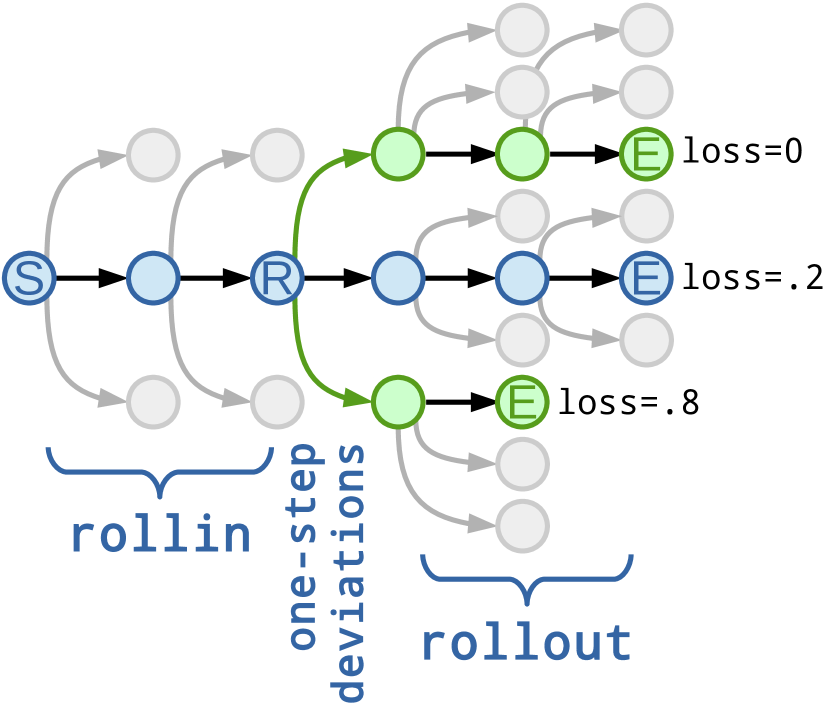
Figure 1: A search space implicitly defined by an imperative program. The system begins at the start state $S$ and chooses the middle among three actions by the rollin policy twice. At state $R$ it considers both the chosen action (middle) and both one-step deviations from that action (top and bottom). Each of these deviations is completed using the rollout policy until an end state is reached, at which point the loss is collected. Here, we learn that deviating to the top action (instead of middle) at state $R$ decreases the loss by $0.2$.

Algorithm 1 shows the code one must write for a part of speech tagger (or generic sequence labeler) under Hamming loss. The only annotation in this code aside from the calls to the library function predict are the computation of an reference (an oracle reference is trivial under Hamming loss) and the computation of the total sequence loss at the end of the function. Note that in this example, the prediction of the tag for the $n$th word depends explicitly on the predictions of all previous words!

The machine learning question that arises is how to learn a good predict function given just this information. The “imperative learning to search” answer [Daumé III et al., 2014] is essentially to run the RunTagger function many times, “trying out” different versions of predict in order to learn one that yields low loss. The challenge is how to do this efficiently. The general strategy is, for some number of epochs, and for each example $(x,y)$ in the training data, to do the following:

1. Execute RunTagger on $x$ with some rollin policy to obtain a search trajectory (sequence of action $\boldsymbol{a}$) and loss $\ell_{0}$

2. Many times:

   1. Choose some time step $t\leq|\boldsymbol{a}|$

   2. Choose an alternative action $a_{t}^{\prime}\neq a_{t}$

   3. Execute RunTagger on $x$, with predict return $a_{1:t-1}$ initially, then $a_{t}^{\prime}$, then acting according to a rollout policy to obtain a new loss $\ell_{t,a_{t}^{\prime}}$

   4. Compare the overall losses $\ell_{0}$ and $\ell_{t,a_{t}^{\prime}}$ to construct a classification/regression example that demonstrates how much better or worse $a_{t}^{\prime}$ is than $a_{t}$ in this context

3. Update the learned policy

Figure 1 shows a schematic of the search space implicitly defined by an imperative program. By executing this program three times (in this example), we are able to explore three different trajectories and compute their losses. These trajectories are defined by the rollin policy (what determines the initial trajectory), the position of one-step deviations (here, state $R$), and the rollout policy (which completes the trajectory after a deviation).

By varying the rollin policy, the rollout policy and the manner in which classification/regression examples are created, this general framework can mimic algorithms like Searn, DAgger and Aggrevate. For instance, DAgger uses rollin=learned policy and rollout=reference, while Searn uses rollin=rollout=stochastic mixture of learned and reference policies.

3 Dependency Parsing by Learning to Search

Action	Configuration
	Stack	Buffer	Arcs
	[Root]	[Flying planes can be dangerous]	{}
Shift	[Root Flying]	[planes can be dangerous]	{}
Reduce-left	[Root]	[planes can be dangerous]	{(planes, Flying)}
Shift	[Root planes]	[can be dangerous]	{(planes, Flying)}
Reduce-left	[Root]	[can be dangerous]	{(planes, Flying), (can, planes)}
Shift	[Root can]	[be dangerous]	{(planes, Flying), (can, planes)}
Shift	[Root can be]	[dangerous]	{(planes, Flying), (can, planes)}
Shift	[Root can be dangerous]	[]	{(planes, Flying), (can, planes)}
Reduce-Right	[Root can be]	[]	{(planes, Flying), (can, planes), (be, dangerous)}
Reduce-Right	[Root can]	[]	{(planes, Flying), (can, planes), (be, dangerous), (can, be)}
Reduce-Right	[Root]	[]	{(planes, Flying), (can, planes), (be, dangerous), (can, be), (Root, can)}

Parse tree derived by the above parser	Gold parse tree

Figure 2: An illustrative example of an arc-hybrid transition parser. The above table show the actions taken and the intermediate configurations generated by a parser. The parse tree derived by the parser is in the bottom left, and the gold parse tree is the bottom right. The distance between these two trees is 2.

Learning to search provides a natural framework for implementing a transition-based dependency parser. A transition-based dependency parser takes a sequence of actions and parses a sentence from left to right by maintaining a stack $S$, a buffer $B$, and a set of dependency arcs $A$. The stack maintains partial parses, the buffer stores the words to be parsed, and $A$ keeps the arcs that have been generated so far. The configuration of the parser at each stage can be defined by a triple $(S,B,A)$. For the ease of notation, we use $w_{p}$ to represent the leftmost word in the buffer and use $s_{1}$ and $s_{2}$ to denote the top and the second top words in the stack. A dependency arc $(w_{h},w_{m})$ is a directed edge that indicates word $w_{h}$ is the parent of word $w_{m}$. When the parser terminates, the arcs in $A$ form a projective dependency tree. We assume that each word only has one parent in the derived dependency parse tree, and use $A[w_{m}]$ to denote the parent of word $w_{m}$. For labeled dependency parsing, we further assign a tag to each arc representing the dependency type between the head and the modifier. For simplicity, we assume an unlabeled parser in the following description. The extension from an unlabeled parser to a labeled parser is straightforward, and is discussed at the end of this section.

Algorithm 2 Trans($S$, $B$, $A$, action)

1:  Let $w_{p}$ be the leftmost element in $B$

2:  if action = Shift then

3:     $S$.push($w_{p}$)

4:     remove $w_{p}$ from $B$

5:  else if action= Reduce-Left then

6:     top $\leftarrow$ $S$.pop()

7:     $A$ $\leftarrow$ $A\cup$ ($w_{p}$,top)

8:  else if action = Reduce-Right then

9:     top $\leftarrow$ $S$.pop()

10:     $A$ $\leftarrow$ $A\cup$ ($S$.top(), top)

11:  end if

12:  return $S,B,A$

We consider an arc-hybrid transition system [Kuhlmann et al., 2011]. In the initial configuration, the buffer $B$ contains all the words in the sentence, a dummy root node is pushed in the stack $S$, and the set of arcs $A$ is empty. The root node cannot be popped out at anytime during parsing. The system then takes a sequence of actions until the buffer is empty and the stack contains only the root node (i.e., $|B|=0$ and $S=\{\textbf{Root}\}$). When the process terminates, a parse tree is derived. At each state, the system can take one of the following actions:

1. Shift: push $w_{p}$ to $S$ and move $p$ to the next word. (Valid when $|B|>0$).

2. Reduce-left: add an arc ($w_{p}$, $s_{1}$) to $A$ and pop $s_{1}$. (Valid when $|B|>0$ and $|S|>1$).

3. Reduce-right: add an arc ($s_{2}$, $s_{1}$) to $A$ and pop $s_{1}$. (Valid when $|S|>1$).

Algorithm 2 shows the execution of these actions during parsing, and Figure 2 demonstrates an example of transition-based dependency parsing.

We can define a search space for dependency parser such that each state represents one configuration during the parsing. The start state is associated with the initial configuration, and the end states are associated with the configurations that $|B|=0$ and $S=\{\textbf{Root}\}$. The loss of each end state is defined by the distance between the derived parse tree and the gold parse tree. The above transition actions define how to move from one search state to the other. In the following, we describe our implementation details.

Algorithm 3 RunParser(sentence)

1:  stack $S$ $\leftarrow$ {Root}

2:  buffer $B$ $\leftarrow$ [words in sentence]

3:  arcs $A$ $\leftarrow$ $\emptyset$

4:  while  $B\neq\emptyset$ or $|S|>1$ do

5:     ValidActs $\leftarrow$ GetValidActions($S,B$)

6:     features $\leftarrow$ GetFeat($S,B,A$)

7:     ref $\leftarrow$ GetGoldAction($S,B$)

8:     action $\leftarrow$ predict(features, ref, ValidActs)

9:     $S,B,A$ $\leftarrow$ Trans($S,B,A$, action)

10:  end while

11:  loss($A[w]$ $\neq$ $A^{*}[w]$, $\forall w\in$ sentence)

12:  return output

Implementation As mentioned in Section 2, to implement a parser using the learning to search framework, we need to provide a decoder, a loss function and reference policy. Thanks to recent work [Goldberg and Nivre, 2013], we know how to compute a “dynamic oracle” reference policy that is optimal. The loss can be measured by how many parents are different between the derived parse tree and the gold annotated parse tree. Algorithm 3 shows the pseudo-code of a decoder for a unlabeled dependency parser. We discuss each subcomponent below.

• GetValidAction returns a set of valid actions that can be taken based on the current configuration.

• GetFeat extracts features based on the current configuration. The features depend on the top few words in the stack and leftmost few words in the buffer as well as their associated part-of-speech tags. We list our feature templates in Table 1. All features are generated dynamically because configuration changes during parsing.

• GetGoldAction implements the dynamic oracle described in [Goldberg and Nivre, 2013]. The dynamic oracle returns the optimal action in any state that leads to the reachable end state with the minimal loss.

• Predict is a library call implemented in the learning to search system. Given training samples, the learning to search system can learn the policy automatically. Therefore, in the test phase, this function returns the predicted action leading to an end state with small structured loss.

• Trans function implements the hybrid-arc transition system. Based on the predicted action and labels, it updates the parser’s configuration, and move the agent to the next search state.

• Loss function is used to measure the distance between the predicted output and the gold annotation. Here, we simply used the number of words for which the parent is wrong as the loss. The Loss has no effect in the test phase.

The above decoder implements an unlabeled parser. To build a labeled parser, when the transition action is Reduce-left or Reduce-right, we call the Predict function again to predict the dependency type of the arc. The loss in the labled dependnecy parser can be measured by $\sum_{w_{i}}loss(w_{i})$, where

$$\begin{split}loss(w_{i})=\begin{cases}2&A[w_{i}]\neq A^{*}[w_{i}]\\ 1&A[w_{i}]=A^{*}[w_{i}],L[w_{i}]\neq L^{*}[w_{i}]\\ 0&\text{Otherwise.}\end{cases}\end{split}$$ (1)

$A[w_{i}]$ and $A^{*}[w_{i}]$ are the parent of $w_{i}$ in the derived parse tree and gold parse tree, respectively, $L[w_{i}]$ is the label assign to the arc $(A[w_{i}],w_{i})$. We observe that this simple loss function performs well empirically.

Unigram Features
$s_{1},s_{2},s_{3},b_{1},b_{2},b_{3},L_{1}(s_{1}),L_{2}(s_{1})$,
$R_{1}(s_{1}),R_{1}(s_{2}),L_{1}(b_{1}),L_{2}(b_{1}),L_{1}(s_{2})$
Bigram Features
$s_{1}s_{1}$, $s_{2}s_{2}$, $s_{3}s_{3}$, $b_{1}b_{1}$, $b_{2}b_{2}$, $b_{3}b_{3}$, $s_{1}b_{1}$,
$s_{1}s_{2}$, $b_{1}b_{2}$
Trigram Features
$s_{1}s_{2}s_{3}$ , $s_{1}b_{1}b_{2}$, $s_{1}s_{2}b_{1}$, $s_{1}b_{1}b_{3}$,
$b_{1}b_{2}b_{3}$ , $s_{1}R_{1}(s_{1})R_{1}(s_{2})$, $s_{1}L_{2}(s_{1})L_{2}(b_{1})$,
$b_{1}L_{1}(b_{1})L_{2}(b_{1})$, $s_{1}s_{2}L_{1}(b_{1})$, $s_{1}b_{1}L_{1}(s_{1})$,
$s_{1}b_{1}L_{1}(s_{2})$, $s_{1}b_{1}L_{1}(b_{1})$

Table 1: Features used in our dependency parsing system. $s_{i}$ represents the $i$-th top element in the stack $S$. $b_{i}$ is the $i$-th leftmost word in the buffer $B$. $L_{i}(w)$ and $R_{i}(w)$ are the $i$-th leftmost child and rightmost child of the word $w$. For each feature template, we includes the surface string and the associated part-of-speech (POS) tag as features. For $R_{i}(w)$ and $L_{i}(w)$, we also include arc labels as features. A feature hashing technique [Weinberger et al., 2009] is employed to provide a fast feature lookup.

We implemented our parser based on an open-source library supporting learning to search. The implementation requires about 300 lines of C++ code. The reduction of implementation effort comes from two-folds. First, in the learning to search framework, there is no need to implement a learning algorithm. Once the decoding function is defined, the system is able to learn the best “Predict” function from training data. Second, L2S provides a unified framework, which allows the library to serve common functions for ease of implementation. For example, quadratic and cubic feature generating functions and a feature hashing mechanism are provided by the library. The unified framework also allows a user to experiment with different base learners and hyper-parameters using command line arguments without modifying the code.

Base Learner As mentioned in Section 2, the learning to search framework reduces structured prediction to cost-sensitive multi-class classification, which can be further reduced to regression. This reduction framework allows us to employ well-studied binary and multi-class classification methods as the base learner. We analyze the value of using more powerful base learners in the experiment section.

4 Experimental Results

While most work compares with MaltParser or MSTParser, which are indeed weak baselines, we compare with two recent strong baselines: the greedy transition-based parser with dynamic oracle [Goldberg and Nivre, 2013] and the Stanford neural network parser [Chen and Manning, 2014]. We evaluate on a wide range of different languages, and show that our parser achieves comparable or better results on all languages, with significantly less engineering.

Parser	Transition	Base learner	Reference
L2S	arc-hybrid	NN	Dynamic
Dyna	arc-hybrid	perceptron	Dynamic
Snn	arc-standard	NN	Static

Table 2: Parser settings.

Parser	Ar	Bu	Ch	Da	Du	En	Ja	Po	Sl	Sw	Avg
	UAS
L2S	77.59	90.64	90.46	88.03	78.06	92.30	90.89	89.77	81.28	89.12	86.81
Dyna	77.89	89.54	89.41	87.37	74.63	91.84	92.72	85.82	77.14	87.85	85.42
Snn	67.37∗	88.05	87.31	82.98	75.34	90.20	89.45	83.19∗	63.60∗	85.70	81.32∗
	LAS
L2S	66.44	85.07	86.43	81.36	73.55	91.09	89.53	84.68	72.48	82.81	81.34
Dyna	66.33	84.73	85.14	82.30	70.26	90.81	90.91	82.00	68.65	82.21	80.33
Snn	51.72∗	84.01	82.72	77.44	71.96	89.10	87.37	77.88∗	51.08∗	80.09	75.34∗

Table 3: UAS and LAS on PTB and CoNLL-X. The average score over all languages is shown in the last column. The best scores for each language is bolded. Snn makes assumptions about the structure of languages and hence obtains substantially worse performance on languages with multi-root trees (marked with ^∗). Excluding these languages, Snn achieves 85.6 (UAS) and 81.8 (LAS) in average, while L2S achieves 88.5 and 84.3.

4.1 Datasets

We conduct experiments on the English Penn Treebank (PTB) [Marcus et al., 1993] and the CoNLL-X [Buchholz and Marsi, 2006] datasets for 9 other languages, including Arabic, Bulgarian, Chinese, Danish, Dutch, Japanese, Portuguese, Slovene and Swedish. For PTB, we convert the constituency trees to dependencies by the head rules of ?). We follow the standard split: sections 2 to 21 for training, section 22 for development and section 23 for testing. The POS tags in the evaluation data is assigned by the Stanford POS tagger [Toutanova et al., 2003], which has an accuracy of 97.2% on the PTB test set. For CoNLL-X, we use the given train/test splits and reserve the last 10% of training data for development if needed. The gold POS tags given in the CoNLL-X datasets are used.

4.2 Setup and Parameters

For L2S, the rollin policy is a mixture of the current (learned) policy and the reference (dynamic oracle) policy. The probability of executing the reference policy decreases over each round. Specifically, we set it to be $1-(1-\alpha)^{t}$, where $t$ is the number of rounds and $\alpha$ is set to $10^{-5}$ in all experiments. It has been shown [Ross and Bagnell, 2014, Chang et al., 2015] that when the reference policy is optimal, it is preferable to roll out with the reference. Therefore, we roll out with the dynamic oracle [Goldberg and Nivre, 2013].

Our base learner is a simple neural network with one hidden layer. The hidden layer size is 5 and we do not use word or POS tag embeddings. We find the Follow-the-Regularized-Leader-Proximal (FTRL) online learning algorithm particularly effective with learning the neural network and simply use default hyperparameters.

We compare with the recent transition-based parser with dynamic oracles (Dyna) [Goldberg and Nivre, 2013], and the Stanford neural network parser (Snn) [Chen and Manning, 2014]. Settings of the three parsers are shown in Table 2.

For Dyna, we use the software provided by the authors online. Our initial experiments show that its performance is the best using the arc hybrid system with exploration parameters $k=1$, $p=1$, thus we use this setting for all experiments. The best model evaluated on the development set among 5 runs with different random seeds are chosen for testing.

For Snn, we use the latest Stanford parser. Since all other parsers do not use external resources, we do not provide pretrained word embeddings and initialize randomly. We use the same parameter values as suggested in [Chen and Manning, 2014], which are also the default settings of the software. The best model over 20000 iterations evaluated on the development set is used for testing.

In addition, we compare with the RedShift parser on PTB. For fair comparison, we only use its basic features (excluding features based on the Brown cluster). We use the default parameters, which runs a beam search with width 8. In our experiments, the RedShift parser has UAS 92.10 and LAS 90.83 on the PTB test set.

4.3 Results

We report unlabeled attachment scores (UAS) and labeled attachment scores (LAS) in Table 3. Punctuation is excluded in all evaluations. Our parser achieves up to 4% improvement on both UAS and LAS. Compared with Dyna, our parser has the same transition system and oracle but more powerful base learners to choose from. Compared with Snn, we use much fewer hidden units and parameters to tune.

Base Leaner	Dev		Test
	UAS	LAS	UAS	LAS
SGD	89.34	88.03	89.34	87.89
SGD+	91.0	89.5	91.0	89.6
NN	92.02	90.78	91.97	90.84
NN+FTRL	92.27	91.04	92.30	91.09
Multiclass	91.7	90.6	91.3	90.2

Table 4: Performance of different base learning algorithms with the L2S parser on PTB corpus.

The Value of Strong Base Learners. L2S allows us to leverage well studied classification methods. We show the performance when training with base learners using the following update rules. Unless stated otherwise all the base learners are cost-sensitive multiclass classifiers.

1. SGD: stochastic gradient descent updates.

2. SGD+: improved update rule using an adaptive metric [Duchi et al., 2011, McMahan and Streeter, 2010], importance invariant updates [Karampatziakis and Langford, 2011], and normalized updates [Ross et al., 2013].

3. NN: a single-hidden-layer neural network with 5 hidden nodes.

4. NN + FTRL: a neural network learner with follow-the-regularized-leader regularization (the base learner in the above experiments).

5. Multiclass: a multiclass classifier using NN+FTRL update rules. The gold label is given by the dynamic oracle.

The results in Table 4 show that using a strong base learner and taking care of low-level learning details (i.e., using cost-sensitive multiclass classifier) can improve the performance.

Base Leaner	Dev		Test
	UAS	LAS	UAS	LAS
Uni-gram	80.41	78.01	80.97	78.65
Uni- + Bi-gram	90.73	89.46	91.08	89.81
All features	92.27	91.04	92.30	91.09

Table 5: The contribution of Bi-gram and Tri-gram features. Results are evaluated on the dev and the test set of PTB.

Finally, Figure 5 shows the performance of different feature templates. Using a comprehensive set of features leads to a better dependency parser.

5 Related Work

Training a transition-based dependency parser can be viewed as an imitation learning problem. However, most early works focus on decoding or feature engineering instead of the core learning algorithm. For a long time, averaged perceptron is the default learner for dependency parsing. ?) first proposed dynamic oracles under the framework of imitation learning. Their approach is essentially a special case of our algorithm: the base learner is a multi-class perceptron, and no rollout is executed to assign cost to actions. In this work, we combine dynamic oracles into learning and explore the search space in a more principled way by learning to search: by cost-sensitive classification, we evaluate the end result of each non-optimal action instead of treating them as equally bad.

There are a number of works that use the L2S approach to solve various other structured prediction problems, for example, sequence labeling [Doppa et al., 2014], coreference resolution [Ma et al., 204], graph-based dependency parsing [He et al., 2013]. However, these works can be considered as a special setting under our unified learning framework, e.g., with a custom action set or different rollin/rollout methods.

To our knowledge, this is the first work that develops a general programming interface for dependency parsing, or more broadly, for structured prediction. Our system bears some resemblance to probabilistic programming language (e.g., [McCallum et al., 2009, Gordon et al., 2014]), however, instead of relying on a new programming language, ours is implemented in C++ and Python, thus is easily accessible.

6 Conclusion and Discussion

We have described a simple transition-based dependency parser based on the learning to search framework. We show that it is now much easier to implement a high-performance dependency parser. Furthermore, we provide a wide range of advanced optimization methods to choose from during training. Experimental results show that we consistently achieve better performance across 10 languages. An interesting direction for future work is to extend the current system beyond greedy search. In addition, there is a large room for speeding up training time by smartly choosing where to rollout.

Function	Number of lines
Setup	90
GetValidActions	17
GetFeat	86
GetGoldAction	41
Trans	28
RunParser	40
Total	331

Table 6: Number of code lines of our dependency parser implementation. The “Setup” contains class constructor, destructor, and handlers for the learning to search framework.

Dependency Parser	Number of lines
L2S (ours)	$\sim$300
Stanford	$\sim$3K
RedShift	$\sim$2K
[Goldberg and Nivre, 2013]	$\sim$4K
Malt Parser	$\sim$10K

Table 7: Number of lines of dependency parser implementations.

We implemented our dependency parser at Vowpal Wabbit (http://hunch.net/~vw/), a machine learning system supporting online learning, hashing, reductions, and L2S. Table 7 shows the number of code lines for each function in our implementation, and Table 7 shows the number of lines of other popular dependency parsing systems. Redshift and ?) are implemented in Python. Stanford and Malt Parser are in Java. Our implementation is in C++. C++ is usually more lengthy than Python and is competitive to Java. The code is readable and contains proper comments as shown below.

⬇

1#include "search_dep_parser.h"

#include "gd.h"

3#include "cost_sensitive.h"

5#define val_namespace 100 // valency and distance feature space

#define offset_const 344429

7

namespace DepParserTask { Search::search_task task = { "dep_parser", run, initialize, finish, setup, nullptr}; }

9

struct task_data {

11 example *ex;

size_t root_label, num_label;

13 v_array<uint32_t> valid_actions, valid_labels, action_loss, gold_heads, gold_tags, stack, heads, tags, temp;

v_array<uint32_t> children[6]; // [0]:num_left_arcs, [1]:num_right_arcs; [2]: leftmost_arc, [3]: second_leftmost_arc, [4]:rightmost_arc, [5]: second_rightmost_arc

15 example * ec_buf[13];

};

17

namespace DepParserTask {

19 using namespace Search;

21 void initialize(Search::search& srn, size_t& num_actions, po::variables_map& vm) {

task_data *data = new task_data();

23 data->action_loss.resize(4,true);

data->ex = NULL;

25 srn.set_num_learners(3);

srn.set_task_data<task_data>(data);

27 po::options_description dparser_opts("dependency parser options");

dparser_opts.add_options()

29 ("root_label", po::value<size_t>(&(data->root_label))->default_value(8), "Ensure that there is only one root in each sentence")

("num_label", po::value<size_t>(&(data->num_label))->default_value(12), "Number of arc labels");

31 srn.add_program_options(vm, dparser_opts);

33 for(size_t i=1; i<=data->num_label;i++)

if(i!=data->root_label)

35 data->valid_labels.push_back(i);

37 data->ex = alloc_examples(sizeof(polylabel), 1);

data->ex->indices.push_back(val_namespace);

39 for(size_t i=1; i<14; i++)

data->ex->indices.push_back((unsigned char)i+’A’);

41 data->ex->indices.push_back(constant_namespace);

43 vw& all = srn.get_vw_pointer_unsafe();

const char* pair[] = {"BC", "BE", "BB", "CC", "DD", "EE", "FF", "GG", "EF", "BH", "BJ", "EL", "dB", "dC", "dD", "dE", "dF", "dG", "dd"};

45 const char* triple[] = {"EFG", "BEF", "BCE", "BCD", "BEL", "ELM", "BHI", "BCC", "BJE", "BHE", "BJK", "BEH", "BEN", "BEJ"};

vector<string> newpairs(pair, pair+19);

47 vector<string> newtriples(triple, triple+14);

all.pairs.swap(newpairs);

49 all.triples.swap(newtriples);

51 srn.set_options(AUTO_CONDITION_FEATURES | NO_CACHING);

srn.set_label_parser( COST_SENSITIVE::cs_label, [](polylabel&l) -> bool { return l.cs.costs.size() == 0; });

53 }

55 void finish(Search::search& srn) {

task_data *data = srn.get_task_data<task_data>();

57 data->valid_actions.delete_v();

data->valid_labels.delete_v();

59 data->gold_heads.delete_v();

data->gold_tags.delete_v();

61 data->stack.delete_v();

data->heads.delete_v();

63 data->tags.delete_v();

data->temp.delete_v();

65 data->action_loss.delete_v();

dealloc_example(COST_SENSITIVE::cs_label.delete_label, *data->ex);

67 free(data->ex);

for (size_t i=0; i<6; i++) data->children[i].delete_v();

69 delete data;

}

71

void inline add_feature(example *ex, uint32_t idx, unsigned char ns, size_t mask, uint32_t multiplier){

73 feature f = {1.0f, (idx * multiplier) & (uint32_t)mask};

ex->atomics[(int)ns].push_back(f);

75 }

77 void inline reset_ex(example *ex){

ex->num_features = 0;

79 ex->total_sum_feat_sq = 0;

for(unsigned char *ns = ex->indices.begin; ns!=ex->indices.end; ns++){

81 ex->sum_feat_sq[(int)*ns] = 0;

ex->atomics[(int)*ns].erase();

83 }

}

85

// arc-hybrid System.

87 uint32_t transition_hybrid(Search::search& srn, uint32_t a_id, uint32_t idx, uint32_t t_id) {

task_data *data = srn.get_task_data<task_data>();

89 v_array<uint32_t> &heads=data->heads, &stack=data->stack, &gold_heads=data->gold_heads, &gold_tags=data->gold_tags, &tags = data->tags;

v_array<uint32_t> *children = data->children;

91 switch(a_id) {

case 1: //SHIFT

93 stack.push_back(idx);

return idx+1;

95 case 2: //RIGHT

heads[stack.last()] = stack[stack.size()-2];

97 children[5][stack[stack.size()-2]]=children[4][stack[stack.size()-2]];

children[4][stack[stack.size()-2]]=stack.last();

99 children[1][stack[stack.size()-2]]++;

tags[stack.last()] = t_id;

101 srn.loss(gold_heads[stack.last()] != heads[stack.last()]?2:(gold_tags[stack.last()] != t_id)?1:0);

stack.pop();

103 return idx;

case 3: //LEFT

105 heads[stack.last()] = idx;

children[3][idx]=children[2][idx];

107 children[2][idx]=stack.last();

children[0][idx]++;

109 tags[stack.last()] = t_id;

srn.loss(gold_heads[stack.last()] != heads[stack.last()]?2:(gold_tags[stack.last()] != t_id)?1:0);

111 stack.pop();

return idx;

113 }

return idx;

115 }

117 void extract_features(Search::search& srn, uint32_t idx, vector<example*> &ec) {

vw& all = srn.get_vw_pointer_unsafe();

119 task_data *data = srn.get_task_data<task_data>();

reset_ex(data->ex);

121 size_t mask = srn.get_mask();

uint32_t multiplier = all.wpp << all.reg.stride_shift;

123 v_array<uint32_t> &stack = data->stack, &tags = data->tags, *children = data->children, &temp=data->temp;

example **ec_buf = data->ec_buf;

125 example &ex = *(data->ex);

127 add_feature(&ex, (uint32_t) constant, constant_namespace, mask, multiplier);

size_t n = ec.size();

129

for(size_t i=0; i<13; i++)

131 ec_buf[i] = nullptr;

133 // feature based on the top three examples in stack ec_buf[0]: s1, ec_buf[1]: s2, ec_buf[2]: s3

for(size_t i=0; i<3; i++)

135 ec_buf[i] = (stack.size()>i && *(stack.end-(i+1))!=0) ? ec[*(stack.end-(i+1))-1] : 0;

137 // features based on examples in string buffer ec_buf[3]: b1, ec_buf[4]: b2, ec_buf[5]: b3

for(size_t i=3; i<6; i++)

139 ec_buf[i] = (idx+(i-3)-1 < n) ? ec[idx+i-3-1] : 0;

141 // features based on the leftmost and the rightmost children of the top element stack ec_buf[6]: sl1, ec_buf[7]: sl2, ec_buf[8]: sr1, ec_buf[9]: sr2;

for(size_t i=6; i<10; i++) {

143 if (!stack.empty() && stack.last() != 0&& children[i-4][stack.last()]!=0)

ec_buf[i] = ec[children[i-4][stack.last()]-1];

145 }

147 // features based on leftmost children of the top element in bufer ec_buf[10]: bl1, ec_buf[11]: bl2

for(size_t i=10; i<12; i++)

149 ec_buf[i] = (idx <=n && children[i-8][idx]!=0)? ec[children[i-8][idx]-1] : 0;

ec_buf[12] = (stack.size()>1 && *(stack.end-2)!=0 && children[2][*(stack.end-2)]!=0)? ec[children[2][*(stack.end-2)]-1]:0;

151

// unigram features

153 uint64_t v0;

for(size_t i=0; i<13; i++) {

155 for (unsigned char* fs = ec[0]->indices.begin; fs != ec[0]->indices.end; fs++) {

if(*fs == constant_namespace) // ignore constant_namespace

157 continue;

159 uint32_t additional_offset = (uint32_t)(i*offset_const);

if(!ec_buf[i]){

161 for(size_t k=0; k<ec[0]->atomics[*fs].size(); k++) {

v0 = affix_constant*((*fs+1)*quadratic_constant + k);

163 add_feature(&ex, (uint32_t) v0 + additional_offset, (unsigned char)((i+1)+’A’), mask, multiplier);

}

165 }

else {

167 for(size_t k=0; k<ec_buf[i]->atomics[*fs].size(); k++) {

v0 = (ec_buf[i]->atomics[*fs][k].weight_index / multiplier);

169 add_feature(&ex, (uint32_t) v0 + additional_offset, (unsigned char)((i+1)+’A’), mask, multiplier);

}

171 }

}

173 }

175 // Other features

temp.resize(10,true);

177 temp[0] = stack.empty()? 0: (idx >n? 1: 2+min(5, idx - stack.last()));

temp[1] = stack.empty()? 1: 1+min(5, children[0][stack.last()]);

179 temp[2] = stack.empty()? 1: 1+min(5, children[1][stack.last()]);

temp[3] = idx>n? 1: 1+min(5 , children[0][idx]);

181 for(size_t i=4; i<8; i++)

temp[i] = (!stack.empty() && children[i-2][stack.last()]!=0)?tags[children[i-2][stack.last()]]:15;

183 for(size_t i=8; i<10; i++)

temp[i] = (idx <=n && children[i-6][idx]!=0)? tags[children[i-6][idx]] : 15;

185

size_t additional_offset = val_namespace*offset_const;

187 for(int j=0; j< 10;j++) {

additional_offset += j* 1023;

189 add_feature(&ex, temp[j]+ additional_offset , val_namespace, mask, multiplier);

}

191

size_t count=0;

193 for (unsigned char* ns = data->ex->indices.begin; ns != data->ex->indices.end; ns++) {

data->ex->sum_feat_sq[(int)*ns] = (float) data->ex->atomics[(int)*ns].size();

195 count+= data->ex->atomics[(int)*ns].size();

}

197 for (vector<string>::iterator i = all.pairs.begin(); i != all.pairs.end();i++)

count += data->ex->atomics[(int)(*i)[0]].size()* data->ex->atomics[(int)(*i)[1]].size();

199 for (vector<string>::iterator i = all.triples.begin(); i != all.triples.end();i++)

count += data->ex->atomics[(int)(*i)[0]].size()*data->ex->atomics[(int)(*i)[1]].size()*data->ex->atomics[(int)(*i)[2]].size();

201 data->ex->num_features = count;

data->ex->total_sum_feat_sq = (float) count;

203 }

205 void get_valid_actions(v_array<uint32_t> & valid_action, uint32_t idx, uint32_t n, uint32_t stack_depth, uint32_t state) {

valid_action.erase();

207 if(idx<=n) // SHIFT

valid_action.push_back(1);

209 if(stack_depth >=2) // RIGHT

valid_action.push_back(2);

211 if(stack_depth >=1 && state!=0 && idx<=n) // LEFT

valid_action.push_back(3);

213 }

215 bool is_valid(uint32_t action, v_array<uint32_t> valid_actions) {

for(size_t i=0; i< valid_actions.size(); i++)

217 if(valid_actions[i] == action)

return true;

219 return false;

}

221

size_t get_gold_actions(Search::search &srn, uint32_t idx, uint32_t n){

223 task_data *data = srn.get_task_data<task_data>();

v_array<uint32_t> &action_loss = data->action_loss, &stack = data->stack, &gold_heads=data->gold_heads, &valid_actions=data->valid_actions;

225

if (is_valid(1,valid_actions) &&( stack.empty() || gold_heads[idx] == stack.last()))

227 return 1;

229 if (is_valid(3,valid_actions) && gold_heads[stack.last()] == idx)

return 3;

231

for(size_t i = 1; i<= 3; i++)

233 action_loss[i] = (is_valid(i,valid_actions))?0:100;

235 for(uint32_t i = 0; i<stack.size()-1; i++)

if(idx <=n && (gold_heads[stack[i]] == idx || gold_heads[idx] == stack[i]))

237 action_loss[1] += 1;

if(stack.size()>0 && gold_heads[stack.last()] == idx)

239 action_loss[1] += 1;

241 for(uint32_t i = idx+1; i<=n; i++)

if(gold_heads[i] == stack.last()|| gold_heads[stack.last()] == i)

243 action_loss[3] +=1;

if(stack.size()>0 && idx <=n && gold_heads[idx] == stack.last())

245 action_loss[3] +=1;

if(stack.size()>=2 && gold_heads[stack.last()] == stack[stack.size()-2])

247 action_loss[3] += 1;

249 if(gold_heads[stack.last()] >=idx)

action_loss[2] +=1;

251 for(uint32_t i = idx; i<=n; i++)

if(gold_heads[i] == stack.last())

253 action_loss[2] +=1;

255 // return the best action

size_t best_action = 1;

257 for(size_t i=1; i<=3; i++)

if(action_loss[i] <= action_loss[best_action])

259 best_action= i;

return best_action;

261 }

263 void setup(Search::search& srn, vector<example*>& ec) {

task_data *data = srn.get_task_data<task_data>();

265 v_array<uint32_t> &gold_heads=data->gold_heads, &heads=data->heads, &gold_tags=data->gold_tags, &tags=data->tags;

uint32_t n = (uint32_t) ec.size();

267 heads.resize(n+1, true);

tags.resize(n+1, true);

269 gold_heads.erase();

gold_heads.push_back(0);

271 gold_tags.erase();

gold_tags.push_back(0);

273 for (size_t i=0; i<n; i++) {

v_array<COST_SENSITIVE::wclass>& costs = ec[i]->l.cs.costs;

275 uint32_t head = (costs.size() == 0) ? 0 : costs[0].class_index;

uint32_t tag = (costs.size() <= 1) ? data->root_label : costs[1].class_index;

277 if (tag > data->num_label) {

cerr << "invalid label " << tag << " which is > num actions=" << data->num_label << endl;

279 throw exception();

}

281 gold_heads.push_back(head);

gold_tags.push_back(tag);

283 heads[i+1] = 0;

tags[i+1] = -1;

285 }

287 for(size_t i=0; i<6; i++)

data->children[i].resize(n+1, true);

289 }

291 void run(Search::search& srn, vector<example*>& ec) {

task_data *data = srn.get_task_data<task_data>();

293 v_array<uint32_t> &stack=data->stack, &gold_heads=data->gold_heads, &valid_actions=data->valid_actions, &heads=data->heads, &gold_tags=data->gold_tags, &tags=data->tags, &valid_labels=data->valid_labels;

uint32_t n = (uint32_t) ec.size();

295

stack.erase();

297 stack.push_back((data->root_label==0)?0:1);

for(size_t i=0; i<6; i++)

299 for(size_t j=0; j<n+1; j++)

data->children[i][j] = 0;

301

int count=1;

303 uint32_t idx = ((data->root_label==0)?1:2);

while(stack.size()>1 || idx <= n){

305 if(srn.predictNeedsExample())

extract_features(srn, idx, ec);

307 get_valid_actions(valid_actions, idx, n, (uint32_t) stack.size(), stack.size()>0?stack.last():0);

uint32_t gold_action = get_gold_actions(srn, idx, n);

309

// Predict the next action {SHIFT, REDUCE_LEFT, REDUCE_RIGHT}

311 count = 2*idx + 1;

uint32_t a_id= Search::predictor(srn, (ptag) count).set_input(*(data->ex)).set_oracle(gold_action).set_allowed(valid_actions).set_condition_range(count-1, srn.get_history_length(), ’p’).set_learner_id(0).predict();

313 count++;

315 uint32_t t_id = 0;

if(a_id ==2 || a_id == 3){

317 uint32_t gold_label = gold_tags[stack.last()];

t_id= Search::predictor(srn, (ptag) count).set_input(*(data->ex)).set_oracle(gold_label).set_allowed(valid_labels).set_condition_range(count-1, srn.get_history_length(), ’p’).set_learner_id(a_id-1).predict();

319 }

count++;

321 idx = transition_hybrid(srn, a_id, idx, t_id);

}

323

heads[stack.last()] = 0;

325 tags[stack.last()] = data->root_label;

srn.loss((gold_heads[stack.last()] != heads[stack.last()]));

327 if (srn.output().good())

for(size_t i=1; i<=n; i++)

329 srn.output() << (heads[i])<<":"<<tags[i] << endl;

}

331}

References

- [Buchholz and Marsi, 2006] Sabine Buchholz and Erwin Marsi. 2006. Conll-x shared task on multilingual dependency parsing. In Proceedings of the Tenth Conference on Computational Natural Language Learning, pages 149–164. Association for Computational Linguistics.
- [Chang et al., 2015] Kai-Wei Chang, Akshay Krishnamurthy, Alekh Agarwal, Hal Daumé III, and John Langford. 2015. Learning to search better than your teacher. arXiv:1502.02206.
- [Chen and Manning, 2014] Danqi Chen and Christopher Manning. 2014. A fast and accurate dependency parser using neural networks. In Proceedings of the Conference on Empirical Methods in Natural Language Processing (EMNLP), pages 740–750.
- [Collins and Roark, 2004] Michael Collins and Brian Roark. 2004. Incremental parsing with the perceptron algorithm. In Proceedings of the Conference of the Association for Computational Linguistics (ACL).
- [Daumé III and Marcu, 2005] Hal Daumé III and Daniel Marcu. 2005. Learning as search optimization: Approximate large margin methods for structured prediction. In Proceedings of the International Conference on Machine Learning (ICML).
- [Daumé III et al., 2009] Hal Daumé III, John Langford, and Daniel Marcu. 2009. Search-based structured prediction. Machine Learning Journal.
- [Daumé III et al., 2014] Hal Daumé III, John Langford, and Stéphane Ross. 2014. Efficient programmable learning to search. arXiv:1406.1837.
- [Doppa et al., 2012] Janardhan Rao Doppa, Alan Fern, and Prasad Tadepalli. 2012. Output space search for structured prediction. In Proceedings of the International Conference on Machine Learning (ICML).
- [Doppa et al., 2014] Janardhan Rao Doppa, Alan Fern, and Prasad Tadepalli. 2014. HC-Search: A learning framework for search-based structured prediction. Journal of Artificial Intelligence Research (JAIR), 50.
- [Duchi et al., 2011] John C. Duchi, Elad Hazan, and Yoram Singer. 2011. Adaptive subgradient methods for online learning and stochastic optimization. Journal of Machine Learning Research, 12:2121–2159.