Percolation games, probabilistic cellular automata, and the hard-core model

Abstract.

Let each site of the square lattice $\mathbb{Z}^{2}$ be independently assigned one of three states: a trap with probability $p$, a target with probability $q$, and open with probability $1-p-q$, where $0<p+q<1$. Consider the following game: a token starts at the origin, and two players take turns to move, where a move consists of moving the token from its current site $x$ to either $x+(0,1)$ or $x+(1,0)$. A player who moves the token to a trap loses the game immediately, while a player who moves the token to a target wins the game immediately. Is there positive probability that the game is drawn with best play – i.e. that neither player can force a win? This is equivalent to the question of ergodicity of a certain family of elementary one-dimensional probabilistic cellular automata (PCA). These automata have been studied in the contexts of enumeration of directed lattice animals, the golden-mean subshift, and the hard-core model, and their ergodicity has been noted as an open problem by several authors. We prove that these PCA are ergodic, and correspondingly that the game on $\mathbb{Z}^{2}$ has no draws.

On the other hand, we prove that certain analogous games do exhibit draws for suitable parameter values on various directed graphs in higher dimensions, including an oriented version of the even sublattice of $\mathbb{Z}^{d}$ in all $d\geq 3$. This is proved via a dimension reduction to a hard-core lattice gas in dimension $d-1$. We show that draws occur whenever the corresponding hard-core model has multiple Gibbs distributions. We conjecture that draws occur also on the standard oriented lattice $\mathbb{Z}^{d}$ for $d\geq 3$, but here our method encounters a fundamental obstacle.

1. Introduction

We introduce and study percolation games on various graphs. For the lattice $\mathbb{Z}^{2}$, we show that the probability of a draw is 0; this is equivalent to proving ergodicity for a certain family of probabilistic cellular automata. In higher dimensions, we prove that draws can occur, by developing a connection to the question of multiplicity of Gibbs distributions for the hard-core model.

1.1. Two dimensional games and ergodicity

Let $p,q\in[0,1)$ with $0\leq p+q\leq 1$. Let each site of $\mathbb{Z}^{2}$ be one of three types: a trap with probability $p$, a target with probability $q$, and open with probability $1-p-q$, independently for different sites. Consider the following two-player game. A token starts at the origin. The players move alternately; if the token is currently at $x$, a move consists of moving it to $x+(0,1)$ or to $x+(1,0)$. If a player moves the token to a trap, that player loses the game immediately. If a player moves the token to a target, that player wins the game immediately. Otherwise (i.e. if the destination site is open), the game continues with the other player’s turn.

The entire random assignment of traps, targets and open sites to $\mathbb{Z}^{2}$ (which we call the percolation configuration) is known to both players at all times. We call this game the percolation game on $\mathbb{Z}^{2}$. We will call the special case $q=0$ (where we have only traps and open sites) the trapping game, and the case $p=0$ (where we have only targets and open sites) the target game.

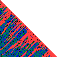
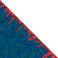
Figure 1. Outcomes of the trapping game ($q=0$) on the finite region $\{x\in\mathbb{Z}_{+}^{2}:x_{1}+x_{2}\leq 200\}$, declaring a draw if the token reaches the diagonal $x_{1}+x_{2}=200$. On the left $p=0.1$ and on the right $p=0.2$. Traps are coloured black, and otherwise colours indicate the outcome when the game is started from that site: first player win (blue); first player loss (green), or draw (red).

If $p+q\geq 1-p_{c}$, where $p_{c}$ is the critical probability for directed site percolation, then, with probability 1, only finitely many sites can be reached from the origin along directed paths of open sites, and so the game must end in finite time. In particular, one or other player must have a winning strategy. (A strategy for one or other player is a map that assigns a legal move, where one exists, to each vertex; a winning strategy is one that results in a win for that player, whatever strategy the other player uses.) Suppose on the other hand that $p+q<1-p_{c}$; is there now a positive probability that neither player has a winning strategy? In that case we say that the game is a draw, with the interpretation that it continues for ever with best play. (When $p=q=0$ the game is clearly always a draw.)

See Figure 1 for simulations on a finite triangular region, with draws imposed as a boundary condition. As the size of this region tends to $\infty$, the probability of a draw starting from the origin converges to the probability of a draw on $\mathbb{Z}^{2}$; the question is whether this limiting probability is positive for any $p$ and $q$.

Related questions are considered in [HM] and [BHMW16], in which the underlying graph is respectively a Galton-Watson tree, and a random subset of the lattice with undirected moves.

In our case of a random subset of $\mathbb{Z}^{2}$ with directed moves, the outcome (first-player win, first-player loss, draw) of the game started from each site can be interpreted in terms of the evolution of a certain one-dimensional discrete-time probabilistic cellular automaton (PCA); the state of the PCA at a given time relates to the outcomes associated to the sites on a given Northwest-Southeast diagonal of $\mathbb{Z}^{2}$.

The PCA has alphabet $\{0,1\}$ and universe $\mathbb{Z}$, so that a configuration at a given time is an element of $\{0,1\}^{\mathbb{Z}}$. (The three game outcomes will correspond to the two states of the PCA via a coupling of two copies of the PCA.) The evolution of the PCA is as follows. Given a configuration $\eta_{t}$ at some time $t$, the configuration $\eta_{t+1}$ at time $t+1$ is obtained by updating each site $n\in\mathbb{Z}$ simultaneously and independently, according to the following rule.

• If $\eta_{t}(n-1)=\eta_{t}(n)=0$, then $\eta_{t+1}(n)$ is set to $0$ with probability $p$ and $1$ with probability $1-p$.

• Otherwise (i.e. if at least one of $\eta_{t}(n-1)$ and $\eta_{t}(n)$ is $1$), $\eta_{t+1}(n)$ is set to $0$ with probability $1-q$ and $1$ with probability $q$.

We denote this PCA $A_{p,q}$. Its evolution rule at each site is illustrated in Figure 2. (The time coordinate $t$ increases from top to bottom, and the spatial coordinate $n$ increases from left to right).

Figure 2. The probabilistic cellular automaton (PCA) $A_{p,q}$.

Formally, we take $A_{p,q}$ to be the operator on the set of distributions on $\{0,1\}^{\mathbb{Z}}$ representing the action of the PCA; if $\mu$ is the distribution of a configuration in $\{0,1\}^{\mathbb{Z}}$, then $A_{p,q}\mu$ is the distribution of the configuration obtained by performing one update step of the PCA. A stationary distribution (or invariant distribution) of a PCA $F$ is a distribution $\mu$ such that $F\mu=\mu$. (More generally, $\mu$ is $k$-periodic if $F^{k}\mu=\mu$, and periodic if it is $k$-periodic for some $k\geq 1$.) A PCA is said to be ergodic if it has a unique stationary distribution and if from any initial distribution, the iterates of the PCA converge to that stationary distribution (in the sense of convergence in distribution with respect to the product topology).

The PCA $A_{p,q}$ has already been studied from a number of different perspectives. It is closely related to the enumeration of directed lattice animals, which are classical objects in combinatorics. More precisely, if $\mu$ is an invariant distribution of $A_{p,q}$, then its marginals satisfy the same recursions as the counting series of directed animals on the square lattice, enumerated according to their area and perimeter. The link was originally made by Dhar [Dha83], and subsequent work includes [BM98, LBM07] – see also Section 4.2 of the survey of Mairesse and Marcovici [MM14a] for a short introduction.

It is quite easy to show that the percolation game has positive probability of a draw if and only if $A_{p,q}$ is non-ergodic (see Proposition 2.2 below). It is also easy to see that $A_{p,q}$ is ergodic whenever $p+q$ is sufficiently large. The question of whether $A_{p,q}$ is ergodic for all $p$ and $q$ has been mentioned as an open problem by several authors – see in particular [TVS⁺90], as well as discussions in [LBM07] and [MM14a].

PCA that are defined on $\mathbb{Z}$ and whose alphabet and neighbourhood are both of size $2$ are sometimes called elementary PCA. A variety of tools have been developed to study their ergodicity. Under the additional assumption of left-right symmetry of the update rule, these PCA are defined by only three parameters: the probabilities to update a cell to state $1$ if its neighbourhood is in state $00$, $11$, or $01$ (which is the same as for $10$). Existing methods can be used to handle more than $90\%$ of the volume of the cube $[0,1]^{3}$ defined by this parameter space, but when $p$ and $q$ are small, the PCA $A_{p,q}$ belongs to an open domain of the cube where none of the previously known criteria hold [TVS⁺90, Chapter 7].

We now state our first main result.

Theorem 1.

If $p>0$ or $q>0$ then the PCA $A_{p,q}$ is ergodic, and the probability of a draw is zero for the percolation game on $\mathbb{Z}^{2}$.

We prove ergodicity by considering the envelope PCA corresponding to $A_{p,q}$, which is a PCA with an expanded alphabet $\{0,{?},1\}$. The envelope PCA corresponds to the status of the game started from each site (with the symbols $0$, ${?}$ and $1$ corresponding to wins, draws and losses respectively). An evolution of the envelope PCA can be used to encode a coupling of two copies of the original PCA, with a ${?}$ symbol denoting sites where the two copies disagree. We introduce a new method involving a positive weight assigned to each ${?}$ symbol (whose value depends on the states of nearby sites). The correct choice of weights is delicate and non-obvious. We show that if the process is translation-invariant, then the average weight per site strictly decreases under the evolution of the envelope PCA, unless it is 0. It follows that any translation-invariant stationary distribution for the envelope PCA has no ${?}$ symbols, with probability 1, and from this we will be able to deduce that the game has no draws with probability 1, so that the original PCA is ergodic. Although the proof of ergodicity could be phrased so as not to refer to games, the notion is useful as a semantic tool and a guide to intuition.

In the particular case $q=0$ (corresponding to the trapping game), it was already known that the PCA has an invariant distribution which is Markovian in space which has made it possible to compute the generating function of directed animals enumerated according to their area alone). This case also has strong connections to the hard-core lattice gas model in statistical physics (which has various applications, for example to the modeling of communications networks) – see Section 3 of this paper. The case $(p,q)=(1/2,0)$ in particular relates to the measure of maximal entropy of the golden mean subshift in dynamical systems – see [Elo96] and also [MM17]. A link between the hard-core PCA $A_{p,0}$ and the trapping game was already mentioned by [LBM07]. As far as we know, the ergodicity of $A_{p,0}$ has not been previously observed. It is a particular case of our Theorem 1, but it also follows from simpler methods which are a special case of those discussed in Section 3.3.

Indeed, for the trapping game, combining the ergodicity of $A_{p,0}$ with the Markovian description of the invariant distribution permits an explicit description of the distribution of game outcomes along a diagonal, as a Markov chain. Consequently, we show that the probability that the first player wins the trapping game is

(1.1) $$\frac{1-2p+\sqrt{\frac{p}{4-3p}}}{2(1-p)}.$$

See Figure 3 for a plot of this winning probability against $p$. The probability is greater than $1/2$ if and only if $p\in(0,1/3)$, and its maximum value is $4-2\surd 3=0.5358...$, attained at $p=(2-\surd 3)/3=0.0893...$.

These methods seemingly do not extend to the case of positive $q$, and we do not know an explicit expression for the win probability (even for the case of the target game, where $p=0$ and $q>0$). Extending further, for a misère version of the trapping game (see Question 4.6 in the final section of the paper) there is apparently no similar connection to a PCA with alphabet $\{0,1\}$, and we do not have a proof that the probability of a draw is 0. This is somewhat reminiscent of the situation for sums of combinatorial games [Con01], where the well-developed theory of “normal play” games extends only in very limited cases to their misère cousins.

Figure 3. The probability that the first player wins the trapping game with $q=0$, conditional on the origin being open, as a function of the density $p$ of traps.

1.2. The trapping game in higher dimensions and the hard-core model

We now consider the particular case $q=0$, and explore extensions of the trapping game, described above for $\mathbb{Z}^{2}$, to more general directed graphs and in particular to lattices in higher dimensions. Theorem 1 tells us that in two dimensions, the probability of a draw is $0$ for all positive $p$, but we find a very different picture in three and higher dimensions.

Let $G=(V,E)$ be a locally finite directed graph. For $x\in V$, let $\operatorname{Out}(x)$ and $\operatorname{In}(x)$ be the sets of out-neighbours and in-neighbours of $x$ respectively. For the trapping game on $G$, let each vertex $x$ be a trap with probability $p$ and open with probability $1-p$, independently for different vertices. A token starts at some vertex, and the two players move alternatively; if the token is currently at $x$, a move consists of moving it to any vertex in $\operatorname{Out}(x)$. The token is only allowed to move to open sites; if all the vertices in $\operatorname{Out}(x)$ are traps, then the player to move loses the game.

For graphs $G$ with an appropriate structure, we develop a connection to the hard-core model on a related undirected graph in one fewer dimensions, to obtain a criterion under which the game is drawn with positive probability.

For an undirected graph with vertex set $W$, and any $\lambda>0$, a Gibbs distribution for the hard-core model on $W$ with activity $\lambda$ is a probability distribution on configurations $\eta\in\{0,1\}^{W}$ such that

(1.2) $$\mathbb{P}\Bigl{(}\eta(v)=1\,\Bigm{|}\,(\eta(w):w\neq v)\Bigr{)}=\begin{cases}\displaystyle\frac{\lambda}{1+\lambda},&\parbox{80.00012pt}{if $\eta(w)=0$ for all\\ neighbours $w$ of $v$;}\\[10.00002pt] 0,&\text{otherwise.}\end{cases}$$

Any such Gibbs distribution is concentrated on configurations $\eta$ that correspond to independent sets, in the sense that no two neighbouring vertices $v$ and $w$ have $\eta(v)=\eta(w)=1$. If $W$ is finite, then there is a unique Gibbs distribution, which is the probability distribution that puts weight proportional to $\prod_{v\in W}\lambda^{\eta(v)}$ on each configuration $\eta$ that is supported on an independent set. However, for infinite graphs, there may be multiple Gibbs distributions. A well-known example is the lattice $\mathbb{Z}^{d}$ with nearest-neighbour edges. For $d=1$, there is a unique Gibbs distribution for all activities $\lambda$. However, for $d\geq 2$, there exist multiple Gibbs distributions when $\lambda$ is sufficiently large [Dob65].

Returning to the trapping game on a directed graph $G$, we now give the key assumptions on $G$ that are required for our dimension reduction method. Suppose there is a partition $(S_{k}:k\in\mathbb{Z})$ of the vertex set $V$ of $G$, and an integer $m\geq 2$, such that the following conditions hold.

• For all $x\in S_{k}$, we have $\operatorname{Out}(x)\subset S_{k+1}\cup\cdots\cup S_{k+m-1}$.

• There is a graph automorphism $\phi$ of $G$ that maps $S_{k}$ to $S_{k+m}$ for every $k$, and such that $\operatorname{Out}(x)=\operatorname{In}(\phi(x))$ for all $x$.

Then let $D_{k}$ be the graph with vertex set $S_{k}\cup\dots\cup S_{k+m-1}$, with an undirected edge $(x,y)$ whenever $(x,y)$ is a (directed) edge of $V$. (Below for convenience we will also use $D_{k}$ to denote the vertex set $S_{k}\cup\dots\cup S_{k+m-1}$.) It is straightforward to show that under conditions (A1) and (A2), the graphs $D_{k}$ are isomorphic to each other for all $k\in\mathbb{Z}$ (see Lemma 3.1); write $D$ for a generic graph which is isomorphic to any of the $D_{k}$. Observe that $D$ is an $m$-partite graph. We have the following criterion for positive probability of draws.

Theorem 2.

Suppose that the directed graph $G$ satisfies (A1) and (A2). If there exist multiple Gibbs distributions for the hard-core model on $D$ with activity $\lambda$, then the trapping game on $G$ with $p=1/(1+\lambda)$ has positive probability of a draw from some vertex.

The simplest case in which to understand the conditions (A1) and (A2) is when $G$ is the directed lattice $\mathbb{Z}^{2}$, with $\operatorname{Out}(x)=\{x+(1,0),x+(0,1)\}$ (the setting of Theorem 1 in Section 1.1). Then we may take the partition of $\mathbb{Z}^{2}$ into Northeast-Southwest diagonals given by $S_{k}:=\{(x_{1},x_{2}):x_{1}+x_{2}=k\}$, along with the bijection $\phi(x)=x+(1,1)$, and $m=2$. The graph $D$ then consists of the vertices of two successive diagonals, and is thus isomorphic to the line $\mathbb{Z}$. (In the context of PCA, $D$ is sometimes called the doubling graph.)

We don’t know whether the converse statement to Theorem 2 holds in general – i.e. whether uniqueness of the Gibbs measure on $D$ implies probability $0$ of a draw. In the case $m=2$, this converse statement does indeed hold – see Section 3.3 for discussion.

As noted above, there is a unique Gibbs distribution for the hard-core model on $\mathbb{Z}$ for all $\lambda>0$. In this case $m=2$, and so the converse statement to Theorem 2 says that there are no draws for any $p\in(0,1)$. This gives an alternative (and perhaps simpler) proof of Theorem 1 in the special case $q=0$.

In higher dimensions the picture is different. We will give several examples of relevant graphs in Section 3.2 and Theorem 3 below. For the current discussion, consider the case where $G$ has vertex set $\mathbb{Z}^{d}_{\text{even}}:=\{x\in\mathbb{Z}^{d}:\sum x_{i}\text{ is even}\}$, with directed edges given by $\operatorname{Out}(x):=\{x\pm e_{i}+e_{d}:1\leq i\leq d-1\}$ (where $e_{i}$ is the $i$th standard basis vector in $\mathbb{Z}^{d}$). So $\operatorname{Out}(x)$ has size $2(d-1)$; any move of the game increases the $d$th coordinate by $1$ and also changes exactly one of the other coordinates by $1$ in either direction. In two dimensions, this game is isomorphic to the original game on $\mathbb{Z}^{2}$. For general $d$, conditions (A1) and (A2) hold with $m=2$ if we set $S_{k}=\{x\in\mathbb{Z}^{d}_{\text{even}}:x_{d}=k\}$ and $\phi(x)=x+2e_{d}$. One then finds that $D$ is isomorphic to the standard $(d-1)$-dimensional cubic lattice $\mathbb{Z}^{d-1}$ with nearest-neighbour edges. As mentioned above, there are multiple Gibbs distributions for the hard-core model on $\mathbb{Z}^{d-1}$ whenever $d\geq 3$ and $\lambda$ is large enough; then Theorem 2 tells us that the trapping game on $G$ has positive probability of a draw when $p$ is sufficiently small. We do not know whether the draw probability is monotone in $p$, nor even whether it is supported on a single interval (giving a single critical point).

To prove Theorem 2, we consider a recursion, analogous to the earlier PCA, expressing game outcomes starting from vertices in $S_{k}$ in terms of outcomes starting in $S_{k+1}\cup\cdots\cup S_{k+m}$. Via the graph isomorphism from $D_{k}$ to $D$, the iteration of this recursion can be reinterpreted as a version of Glauber dynamics for the hard-core model on $D$. If the hard-core model has multiple Gibbs distributions, then they correspond to multiple stationary distributions for the recursion on $G$, and from this we will deduce that draws occur.

Unfortunately, the following very natural example is not amenable to our methods. Let $G$ be the standard cubic lattice $\mathbb{Z}^{d}$ with edge orientations given by $\operatorname{Out}(x)=\{x+e_{i}:1\leq i\leq d\}$. Theorem 2 does not apply for $d\geq 3$, because there is no choice of $m$ and the automorphism $\phi$ such that (A2) holds. We conjecture that, nonetheless, the trapping game has positive probability of a draw whenever $p$ is sufficiently small.

1.3. Further background

The celebrated positive rates conjecture is the assertion that in one dimension, any finite-state finite-range PCA is ergodic, provided the transition probability to any state given any neighbourhood states is positive (the “positive rates” condition). This contrasts with two and higher dimensions, where for example Glauber dynamics for the low-temperature Ising model are well known to be non-ergodic. Despite persuasive heuristic arguments in favour of the positive rates conjecture, Gács [Gác01] has presented an extremely complicated one-dimensional PCA refuting it. (See also [Gra01].) However, it is still natural to hypothesize that all “sufficiently simple” one-dimensional PCA with positive rates are ergodic.

The PCA $A_{p,q}$ satisfies the positive rates condition whenever both $p$ and $q$ are strictly positive. If $p=0$ or $q=0$, although we no longer have positive rates, similar but weaker conditions do hold; $\{0,1\}^{n}$ has positive probability of yielding any word in $\{0,1\}^{n-2}$ after two steps of the evolution. In light of this and the above remarks, it would have been very surprising if these PCA were not ergodic. Nonetheless, proving ergodicity is often very difficult, even in cases where it appears clear from heuristics or simulations.

Another case in point is the notorious noisy majority model on $\mathbb{Z}^{d}$. Here, a configuration is an element of $\{0,1\}^{\mathbb{Z}^{d}}$. The update rule is that with probability $1-p$, a site adopts the more popular value in $\{0,1\}$ among itself and its $2d$ neighbours; with probability $p$ it adopts the other value. In dimensions $d\geq 2$ it is expected that this PCA should behave similarly to the Ising model: it should be ergodic for $p$ sufficiently close to $1/2$, and non-ergodic for $p$ sufficiently small, with a unique critical point separating the two regimes. However, proving any of this appears very challenging. See e.g. [BBJW10, Gra01] and the references therein for more information. One key difficulty with the noisy majority model is the lack of reversibility of the dynamics (in contrast to the Glauber dynamics for the Ising model, for example). This can be compared to the difficulty of obtaining a result like Theorem 2 in the absence of conditions such as (A1) and (A2); see the discussion above at the end of Subsection 1.2.

In a different direction, a variant of the notion of envelope cellular automata has recently been combined with percolation ideas in [GH15], to prove the surprising fact that certain deterministic one-dimensional cellular automata exhibit order from typical finitely supported initial conditions, but disorder from exceptional initial conditions.

1.4. Organization of the paper

In Section 2 we explain the link between the PCA $A_{p,q}$ and the percolation game in $\mathbb{Z}^{2}$. We also establish several basic results concerning monotonicity and ergodicity. The local weighting on configurations is introduced in Subsection 2.2, and the proof of ergodicity is then given in Subsection 2.3.

The relation between the trapping game and the hard-core model is then developed in Section 3. We start by considering the case of $\mathbb{Z}^{2}$ where the ideas are simplest, and in particular we will derive the formula (1.1) for the winning probability. The case of a more general graph is then treated in Subsection 3.2, where Theorem 2 is proved. The converse to Theorem 2 is discussed in Subsection 3.3. In Subsection 3.4 and Theorem 3, we give a variety of examples of the application of Theorem 2 to graphs with vertex set $\mathbb{Z}^{d}$ for $d\geq 3$, for which the role of the doubling graph $D$ is played by various lattice structures. We also give an extension of Theorem 2 in Proposition 3.1 in Subsection 3.5, using a variant form of the correspondence to the hard-core model.

We conclude in Section 4 with some open problems.

2. Percolation games and probabilistic cellular automata

2.1. The PCA for the percolation game

Consider the percolation game on $\mathbb{Z}^{2}$ as defined in the introduction.

Suppose $x$ is an open site of $\mathbb{Z}^{2}$. Let $\eta(x)$ be $\mathrm{W}$, $\mathrm{L}$ or $\mathrm{D}$ according to whether the game started with the token at $x$ is win for the first player, a loss for the first player, or a draw, respectively. (Recall that we assume optimal play, with the players able to see entire percolation configuration when deciding on their strategies). If $x$ is a trap, it is convenient to set $\eta(x)=\mathrm{W}$ (we can imagine that a player is allowed to move the token to $x$, but with the effect that the game is then declared an immediate win for the opponent); similarly if $x$ is a target then we set $\eta(x)=\mathrm{L}$.

Recall that $\operatorname{Out}(x)=\{x+e_{1},x+e_{2}\}$ is the set of sites to which the token can move from $x$. By considering the first move, we have the following recursion for the status of the sites:

(2.1) $$\text{$x$ a trap}\;\Rightarrow\;\eta(x) =\mathrm{W};$$

$$\text{$x$ a target}\;\Rightarrow\;\eta(x) =\mathrm{L};$$

$$\text{$x$ open}\;\Rightarrow\;\eta(x) =\begin{cases}\mathrm{L}&\text{if }\eta(y)=\mathrm{W}\text{ for all }y\in\operatorname{Out}(x)\\ \mathrm{W}&\text{if }\eta(y)=\mathrm{L}\text{ for some }y\in\operatorname{Out}(x)\\ \mathrm{D}&\text{otherwise.}\end{cases}$$

For $k\in\mathbb{Z}$, let $S_{k}$ be the set $\{x=(x_{1},x_{2})\in\mathbb{Z}^{2}:x_{1}+x_{2}=k\}$, a NW-SE diagonal of $\mathbb{Z}^{2}$. The recursion (2.1) gives us the values $(\eta(x):x\in S_{k})$ in terms of the values $(\eta(x):x\in S_{k+1})$ together with the information about which sites in $S_{k}$ are traps.

It is important to note that it is not a priori clear whether the recursion (2.1) suffices to determine $\eta$ uniquely from the percolation configuration. Indeed, in the trivial case $p=q=0$ when all sites are open, we have $\eta(x)=\mathrm{D}$ for all $x$, but (2.1) has other solutions: one is to set $\eta^{\prime}(x)$ equal to $\mathrm{L}$ or $\mathrm{W}$ according to whether $x_{1}+x_{2}$ is odd or even. Such considerations are in fact central to many of our arguments. One way to interpret our main result, Theorem 1, is as saying that (2.1) does have a unique solution almost surely whenever $p$ or $q$ is positive. In contrast, for the higher dimensional variants considered later, the analogous recursions admit multiple solutions for certain parameter values.

Via (2.1), we can regard the configurations on successive diagonals $S_{k}$, as $k$ decreases, as successive states of a one-dimensional PCA. Let us introduce the following recoding:

$$\mathrm{W}=0,\quad\mathrm{L}=1,\quad\mathrm{D}={?}.$$

(In the coupling arguments below, the symbol ${?}$ will be interpreted as marking a site at which the value is “unknown”. The choice to assign $\mathrm{W}=0$ and $\mathrm{L}=1$, rather than the other way around, say, will be important for the later connection with hard-core models.) The PCA evolves as follows: given the values for sites in $S_{k+1}$, each value $\eta(x)$ for $x\in S_{k}$ is derived independently using the values $\eta(x+e_{1})$ and $\eta(x+e_{2})$, according to the scheme given in Figure 4 (where a $*$ represents an arbitrary symbol in $\{0,{?},1\}$).

Figure 4. The PCA $F_{p,q}$ ($*$ denotes an arbitrary symbol).

We denote the corresponding PCA $F_{p,q}$. Although we have defined it as a process in the plane, we can also regard it as a PCA on $\mathbb{Z}$ with a configuration in $\{0,{?},1\}^{\mathbb{Z}}$ evolving in time by setting

(2.2) $$\eta_{t}(n)=\eta\bigl{(}(-t-n,n)\bigr{)}.$$

(Here we have made the arbitrary choice to offset leftward as time increases,so that the PCA rule gives $\eta_{t+1}(n)$ in terms of $\eta_{t}(n)$ and $\eta_{t}(n+1)$.) As in Section 1.1, formally we take $F_{p,q}$ to be an operator on the set of distributions on $\{0,{?},1\}^{\mathbb{Z}}$ representing the action of the PCA.

In the setting of the percolation game, translation invariance of the whole process on $\mathbb{Z}^{2}$ implies that the distribution of the configuration on the diagonal $S_{k}$ does not depend on $k$; that is, the distribution of $\big{(}\eta((k-n,n)):n\in\mathbb{Z}\big{)}$ does not depend on $k$ and is a stationary distribution of $F_{p,q}$. In addition, this distribution is itself invariant under the action of translations of $\mathbb{Z}$.

We next note two useful monotonicity properties for the PCA $F_{p,q}$. In terms of the game, they have natural interpretations: (i) an advantage for one player translates to a disadvantage for the other; and (ii) declaring draws at some positions can only result in more draws elsewhere.

Lemma 2.1.

Let $\mu$ and $\nu$ be probability distributions on $\{0,{?},1\}^{\mathbb{Z}}$.

• If $\mu\leq\nu$, where $\leq$ denotes stochastic domination with respect to the coordinatewise partial order induced by $0<{?}<1$, then $F_{p,q}\mu\geq F_{p,q}\nu$. (Note the reversal of the inequality).

• If $\mu\trianglelefteq\nu$, where $\trianglelefteq$ denotes stochastic domination with respect to the coordinatewise partial order induced by $0\vartriangleleft{?}\vartriangleright 1$, then $F_{p,q}\mu\trianglelefteq F_{p,q}\nu$.

Proof.

We can use the recursion (2.1) to give a coupling of a single step of the PCA $F_{p,q}$ started from two different configurations. Suppose we fix values $(\eta(x):x\in S_{k+1})$ and $(\widetilde{\eta}(x):x\in S_{k+1})$, in such a way that $\eta(x)\leq\widetilde{\eta}(x)$ for all $x\in S_{k+1}$ (where $\leq$ is the coordinatewise order on configurations induced by $0<{?}<1$). Now use (2.1) to obtain values $\eta(x)$ and $\widetilde{\eta}(x)$ for $x\in S_{k}$, using the same realization of traps, targets, and open sites in $S_{k}$ in each case. It is straightforward to check that in that case $\eta(x)\geq\widetilde{\eta}(x)$ for each $x\in S_{k}$. Hence the operator $F_{p,q}$ is decreasing in the desired sense.

Similarly, if $\eta(x)\trianglelefteq\widetilde{\eta}(x)$ for all $x\in S_{k+1}$, then we obtain $\eta(x)\trianglelefteq\widetilde{\eta}(x)$ also for each $x\in S_{k}$. So in this case the operator $F_{p,q}$ is increasing as desired. ∎

If we restrict the PCA $F_{p,q}$ to configurations that do not contain the symbol ${?}$, we recover precisely the binary PCA $A_{p,q}$ defined in the introduction. In the terminology of Bušić et al. [BMM13], the PCA $F_{p,q}$ is the envelope PCA of $A_{p,q}$. A copy of the PCA $F_{p,q}$ can be used to represent a coupling of two or more copies of the PCA $A_{p,q}$, started from different initial conditions. The symbol ${?}$ represents a site whose value is not known, i.e. one which may differ between the different copies.

Specifically, consider starting copies of the hard-core PCA $A_{p,q}$ from several different initial conditions, represented by configurations on the diagonal $S_{k}$ for some fixed $k$. As in the proof of Lemma 2.1, a natural coupling is provided by the recursion (2.1), using the same realization of traps, targets, and open sites in $(S_{r}:r<k)$. In particular, let $k>0$ and consider three copies $\eta$, $\widetilde{\eta}$ and $\eta^{?}$, with $\eta$ and $\widetilde{\eta}$ started from arbitrary initial conditions on $S_{k}$, while $\eta^{?}(x)={?}$ for all $x\in S_{k}$ (so that $\eta^{?}$ is maximal for the ordering $\trianglelefteq$ in Lemma 2.1(ii)). Then we have that $\eta(x)\trianglelefteq\eta^{?}(x)$ and $\widetilde{\eta}(x)\trianglelefteq\eta^{?}(x)$ for all $x\in S_{r}$ with $r<k$. This implies that if $\eta(x)\neq\widetilde{\eta}(x)$, then $\eta^{?}(x)={?}$.

In terms of the game, we have the following interpretation: if the origin $O=(0,0)$ is an open site, and $\eta^{?}(O)=0$ (respectively $\eta^{?}(O)=1$) then the first (respectively second) player can force a win within at most $k$ moves of the game.

The ergodicity of an envelope PCA implies the ergodicity of the original PCA, but the converse is not true in general. In our case, however, we can use the monotonicity property in Lemma 2.1(i) to show that the two are equivalent.

Proposition 2.1.

The PCA $F_{p,q}$ is ergodic if and only if $A_{p,q}$ is ergodic.

Proof.

It is clear from the definitions that if $F_{p,q}$ is ergodic, then $A_{p,q}$ is also ergodic. Conversely, suppose that $A_{p,q}$ is ergodic. Let $\mu$ be a distribution on $\{0,{?},1\}^{\mathbb{Z}}$, and let $\delta_{0}$ and $\delta_{1}$ the distributions concentrated on the states “all $0$s” and “all $1$s”. Then $\delta_{0}\leq\mu\leq\delta_{1}$, so by Lemma 2.1(i), for $k\geq 0$ we have either $F_{p,q}^{k}\delta_{0}\leq F_{p,q}^{k}\mu\leq F_{p,q}^{k}\delta_{1}$ or $F_{p,q}^{k}\delta_{0}\geq F_{p,q}^{k}\mu\geq F_{p,q}^{k}\delta_{1}$, according to whether $k$ is even or odd. But $F_{p,q}^{k}\delta_{0}=A_{p,q}^{k}\delta_{0}$ and $F_{p,q}^{k}\delta_{1}=A_{p,q}^{k}\delta_{1}$, and by ergodicity of $A_{p,q}$, the latter two sequences converge as $k\to\infty$ to the same distribution $\pi$, so $F_{p,q}^{k}\mu$ also converges to $\pi$. Thus $F_{p,q}$ is also ergodic. ∎

Proposition 2.2.

For each $p$ and $q$, the percolation game has probability $0$ of a draw if and only if $A_{p,q}$ is ergodic.

Proof.

If $A_{p,q}$ is ergodic then so is $F_{p,q}$, and so the unique invariant distribution of $F_{p,q}$ has no ${?}$ symbols. But we know that the distribution of the game outcomes along a diagonal $S_{k}$ is invariant for $F_{p,q}$. Hence with probability 1, there are no sites from which the game is drawn.

For the converse, let $\omega$ be a random percolation configuration on $\mathbb{Z}^{2}$. Consider any site $x\in S_{0}$. If the game started from $x$ is not a draw, then (since at each turn the player to move has only finitely many options) one player has a strategy that guarantees a win in fewer than $N$ moves, where $N\in\mathbb{N}$ is a finite random variable that depends on $\omega$. Consequently, if we assign any configuration of states $0,{?},1$ to $S_{N}$ and compute the resulting states on $(S_{n}:0\leq n<N)$ using the recursion (2.1) and the percolation configuration $\omega$, the resulting state at $x$ is the same as its state for the percolation game on $\mathbb{Z}^{2}$ with percolation configuration $\omega$.

Let $\gamma$ be the random configuration of game outcomes on $S_{0}$ arising from $\omega$. Also, fix a distribution $\nu$ on $\{0,1\}^{\mathbb{Z}}$, and let $\gamma_{n}$ be the configuration on $S_{0}$ that results from assigning a configuration with law $\nu$ to $S_{n}$, independent of $\omega$, and applying (2.1) as described above. By the argument in the previous paragraph, if the probability of a draw is 0, then $\gamma_{n}$ converges almost surely to $\gamma$ (in the product topology). Hence also the distribution of $\gamma_{n}$ converges to that of $\gamma$. But $\gamma_{n}$ has distribution $A_{p,q}^{n}\nu$, so $A_{p,q}^{n}\nu$ converges as $n\to\infty$ to the distribution of $\gamma$, which does not depend on $\nu$. Hence $A_{p,q}$ is ergodic. ∎

2.2. The weight function

We are concerned with the PCA $A_{p,q}$ on the alphabet $\{0,1\}$, shown in Figure 2, along with its envelope PCA $F_{p,q}$ shown in Figure 4.

In order to prove the ergodicity of $F_{p,q}$, we will introduce an appropriate weight on ${?}$ symbols, and prove that this weight decreases under the action of $F_{p,q}$. The aim of the present section is to motivate the choice of that special weight system.

Figure 5. The deterministic cellular automaton $F_{0,0}$.

We say that the distribution of a configuration $\eta=(\eta_{i}:i\in\mathbb{Z})$ is shift-invariant if $\eta$ and $(\eta_{i+k}:i\in\mathbb{Z})$ have the same distribution for each $k\in\mathbb{Z}$, and reflection-invariant if $\eta$ and $(\eta_{-i}:i\in\mathbb{Z})$ have the same distribution. If $\mu$ is a distribution and $y\in\{0,{?},1\}^{n}$ is a finite word, we write $\mu(y):=\mu\{\eta:(\eta_{1},\ldots,\eta_{n})=y\}$ for the corresponding cylinder probability.

For shift-invariant distributions $\mu$ on $\{0,{?},1\}^{\mathbb{Z}}$, we introduce the weight function $w$ defined by

(2.3) $$w(\mu)=\mu({?}01)+\mu({?}0)+\mu({?})-(p+q)\,\mu(?*1).$$

To prove Proposition 2.3 we will establish the inequality

(2.4) $$w(F_{p,q}\mu)\leq w(\mu)-(p+q)\mu(?01),$$

for any shift-invariant and reflection-invariant distribution $\mu$. This inequality will indeed ensure that if $\mu$ is $F_{p,q}$-invariant, then $\mu(?01)=0$, which will imply in turn that $\mu(?)=0$.

To give some intuition for the proof of (2.4), let us focus on the case $p=q=0$. Then the PCA $F_{0,0}$ is in fact deterministic (see Figure 5). Suppose $\mu$ is shift-invariant and reflection-invariant. By looking at the possible pre-images of each pattern, we obtain the following three equalities:

$$F_{0,0}\,\mu({?}) =\mu({?}{?})+\mu(0{?})+\mu({?}0),$$

$$F_{0,0}\,\mu({?}0) =\mu({?}{?}1)+\mu(0{?}1)+\mu({?}01),$$

$$F_{0,0}\,\mu({?}01) =0.$$

Observe that:

$$\mu({?}{?})+\mu({?}0)+\mu({?}{?}1)+\mu(0{?}1)=\mu({*}{?}{?})+\mu({*}{?}0)+\mu({?}{?}1)+\mu(0{?}1)\leq\mu({?}),$$

where ${*}$ represents an unspecified symbol to be summed over. Using reflection invariance to deduce $\mu(0{?})=\mu({?}0)$, we then obtain that $w(F_{p,q}\mu)\leq w(\mu)$.

In this deterministic case, we can interpret the weight $w(\mu)$ as assigning a weight to each occurrence of the symbol ${?}$ as follows:

• if a ${?}$ is followed by a $01$, then it receives weight $3$;

• if a ${?}$ is followed by a $0$ and then by something other than a $1$, it receives weight $2$;

• otherwise, a ${?}$ receives weight $1$.

For a shift-invariant distribution $\mu$, $w(\mu)$ is then the expected weight per site under $\mu$.

Let us now consider a symmetric version of the weight system that we have introduced: for each symbol ${?}$, we add its right-weight, as introduced above, to its left-weight, which is equal to $3$ if it the previous letter is a $0$ and if there is a $1$ before it (pattern $10{?})$, to $2$ if the previous letter is a $0$ and if there is something else than a $1$ before, and to $1$ otherwise.

Thus, the weight of the symbol ${?}$ in the pattern $1{?}1$ is equal to $1+1=2$, while in the pattern $10{?}{?}1$, the weight of the first ${?}$ symbol is $3$ (left) $+$ $1$ (right) $=4$, and the weight of the second one is equal to $1+1=2$.

Figure 6 shows an example of an evolution of the deterministic CA $F_{0,0}$ from an initial configuration represented at the top (with time going down the page). The symmetrized weights of the symbols ${?}$ appearing in the space-time diagram are shown in red. As illustrated in the figure, from a pattern $1{?}1$, the symbol ${?}$ disappears and the weight thus decreases, but in other cases the total weight is locally preserved. Indeed, one can check that starting from any initial configuration containing finitely many ${?}$ symbols, the total weight is non-increasing under the action of $F_{0,0}$.

Moving to the general case, allowing $p$ and $q$ to be positive can be interpreted as introducing “mutations” into the determinstic evolution described by $F_{0,0}$, which we control by introducing the final term into the definition of the weight $w$ in (2.3).

Figure 6. Example of evolution of the weight of a configuration under the operator $F_{0,0}$. Time runs down the page, and the weight of each ${?}$ symbol is given below it.

2.3. Proof of ergodicity

Proposition 2.3.

For any $p$ and $q$, the PCA $F_{p,q}$ has no stationary distribution in which the symbol ${?}$ appears with positive probability.

Proof.

It suffices to show that there is no shift-invariant and reflection-invariant stationary distribution in which the symbol ${?}$ appears with positive probability. For consider iterating the PCA starting from the distribution $\delta_{{?}}$ concentrated on the configuration with ${?}$ at all sites. By Lemma 2.1(ii), the probability $F_{p,q}^{n}\delta_{{?}}({?})$ is non-increasing, and if there is any stationary distribution $\mu$ with positive probability of ${?}$, then $F_{p,q}^{n}\delta_{{?}}({?})$ is bounded below by $\mu({?})$ for all $n$, and so does not converge to 0. Then any limit point of the sequence of Césaro sums of $F_{p,q}^{n}\delta_{{?}}$ is a stationary distribution that has positive probability of ${?}$, and that is also shift-invariant and reflection-symmetric.

The idea will be to compare the weight function $w$ defined at (2.3) before and after applying a step of the evolution.

To shorten the proof, we write $\widehat{{*}{*}}$ for a pair of consecutive symbols to be summed over the three possibilities $?0,0?,??$ (i.e. the pairs which can lead to a $?$ at the next step), so that for example $\mu(\widehat{{*}{*}}1)=\mu(?01)+\mu(0?1)+\mu(??1)$. We also write $r=1-p-q$.

Suppose $\mu$ is a shift-invariant distribution. Then we have the equalities

$$F_{p,q}\,\mu(?) =r\mu(\widehat{{*}{*}});$$

$$F_{p,q}\,\mu(?0) =rp\bigl{[}\mu(\widehat{{*}{*}}0)+\mu(\widehat{{*}{*}}?)\bigr{]}+r(1-q)\mu(\widehat{{*}{*}}1);$$

(2.5) $$F_{p,q}\,\mu(?01) =rp(1-p)\mu(\widehat{{*}{*}}00)+rpq\bigl{[}\mu(\widehat{{*}{*}}0?)+\mu(\widehat{{*}{*}}01)+\mu(\widehat{{*}{*}}?)\bigr{]}$$

$$\hskip 133.72786pt+r(1-q)q\mu(\widehat{{*}{*}}1)$$

$$=r^{2}p\mu(\widehat{{*}{*}}00)+rpq\bigl{[}\mu(\widehat{{*}{*}}0)+\mu(\widehat{{*}{*}}?)\bigr{]}+r(1-q)q\mu(\widehat{{*}{*}}1).$$

Summing these three equalities gives

$$F_{p,q}\,\mu(?)+F_{p,q}\,\mu(?0)+F_{p,q}\,\mu(?01)$$

$$=r\mu(\widehat{{*}{*}})+rp(1+q)\bigl{[}\mu(\widehat{{*}{*}}0)+\mu(\widehat{{*}{*}}?)\bigr{]}+r(1-q)(1+q)\mu(\widehat{{*}{*}}1)+r^{2}p\mu(\widehat{{*}{*}}00)$$

$$\leq r\mu(\widehat{{*}{*}})+(p+q)\bigl{[}\mu(\widehat{{*}{*}}0)+\mu(\widehat{{*}{*}}?)\bigr{]}+r\mu(\widehat{{*}{*}}1)+r^{2}(p+q)\mu(\widehat{{*}{*}}00)$$

Suppose in addition that $\mu$ is reflection-invariant. Then

$$\mu(\widehat{{*}{*}})+\mu(\widehat{{*}{*}}1) \leq\mu(0?)+\mu(?0)+\mu(??)+\mu(?1)+\mu(?01)$$

$$\leq\mu(?)+\mu(0?)+\mu(?01)$$

$$=\mu(?)+\mu(?0)+\mu(?01).$$

Substituting into the previous equality gives:

$$F_{p,q}\,\mu(?)+F_{p,q}\,\mu(?0)+F_{p,q}\,\mu(?01)$$

$$\leq r\bigl{[}\mu(?)+\mu(?0)+\mu(?01)\bigr{]}+(p+q)\bigl{[}\mu(\widehat{{*}{*}}0)+\mu(\widehat{{*}{*}}?)\bigr{]}+r^{2}(p+q)\mu(\widehat{{*}{*}}00).$$

To deal with the last term on the right, observe that:

$$F_{p,q}\,\mu(?{*}1)\geq r(1-p)\mu(\widehat{{*}{*}}00)\geq r^{2}\mu(\widehat{{*}{*}}00).$$

It follows that:

$$w(F_{p,q}\mu) =F_{p,q}\,\mu(?)+F_{p,q}\,\mu(?0)+F_{p,q}\,\mu(?01)-(p+q)F_{p,q}\,\mu(?*1)$$

$$\leq r\bigl{[}\mu(?)+\mu(?0)+\mu(?01)\bigr{]}+(p+q)\bigl{[}\mu(\widehat{{*}{*}}0)+\mu(\widehat{{*}{*}}?)\bigr{]}$$

$$=\mu(?)+\mu(?0)+\mu(?01)$$

$$\hskip 56.9055pt+(p+q)\bigl{[}\mu(\widehat{{*}{*}}0)+\mu(\widehat{{*}{*}}?)-\mu(?)-\mu(?0)-\mu(?01)\bigr{]}$$

$$\leq\mu(?)+\mu(?0)+\mu(?01)-(p+q)\mu(?*1)-(p+q)\mu(?01)$$

(2.6) $$=w(\mu)-(p+q)\mu(?01).$$

The last inequality comes from

$$\mu(\widehat{{*}{*}}0)+\mu(\widehat{{*}{*}}?)+\mu(?{*}1) \leq\mu(?{*}0)+\mu(0?0)+\mu(?{*}?)+\mu(0??)+\mu(?{*}1)$$

$$\leq\mu(?)+\mu(0?).$$

Finally suppose that $\mu$ is $F_{p,q}$-invariant. Then since $p+q>0$, it follows from (2.6) that that $\mu(?01)=0$. This must imply that $\mu(?)=0$. To explain why, let us first consider the case $p,q>0$. Then, from $0=\mu(?01)=F_{p,q}\,\mu(?01)\geq rpq\,\mu(\widehat{{*}{*}}),$ we obtain $\mu(\widehat{{*}{*}})=0$, and then $\mu(?)=F_{p,q}\,\mu(?)=r\mu(\widehat{{*}{*}})=0$. In the case $p=0$ and $q>0$, using the equations of (2.5), we get, successively,

$$0=\mu(?01)= F_{0,q}\,\mu(?01)=(1-q)^{2}q\,\mu(\widehat{{*}{*}}1),$$

$$\mu(?0)= F_{0,q}\,\mu(?0)=(1-q)^{2}\mu(\widehat{{*}{*}}1)=0,$$

$$\mu(?)= F_{0,q}\,\mu(?)=(1-q)\mu(\widehat{{*}{*}})=(1-q)\mu(??)\leq(1-q)\mu(?),$$

so that we also deduce that $\mu(?)=0$. A similar argument applies in the case when $p>0$ and $q=0$. ∎

Now, we can quickly deduce our main result.

Proof of Theorem 1.

We know that the distribution of the states (win, loss, draw) of the sites along a diagonal $S_{k}$ in the percolation game is a stationary distribution for $F_{p,q}$. Since by Proposition 2.3, $F_{p,q}$ has no stationary distribution with positive probability of ${?}$ whenever $p+q>0$, the probability of a draw in the percolation game must be $0$. Then by Proposition 2.2, the PCA $A_{p,q}$ is ergodic for each $p$ and $q$ with $p+q>0$. ∎

3. Trapping games and the hard-core model

3.1. The two-dimensional case

In this section we develop the relationship between the trapping game and the hard-core model. We start in the setting of $\mathbb{Z}^{2}$ where the ideas are easiest to understand, but our main application will be in Section 3.2, when we establish a more general framework, and apply it to show that certain higher-dimensional games have positive probability of a draw when $p$ is sufficiently small.

Consider the hard-core PCA $A_{p,0}$. This PCA is known to belong to a family of one-dimensional PCA having a stationary distribution that is itself a stationary Markov chain indexed by $\mathbb{Z}$ [BGM69, TVS⁺90, MM14b]. This distribution, $\mu_{p}$ say, is the law of the stationary Markov chain on $\mathbb{Z}$ with transition matrix

(3.1) $$P=\begin{pmatrix}p_{0,0}&p_{0,1}\\ p_{1,0}&p_{1,1}\end{pmatrix}=\begin{pmatrix}{\frac{2-p-\sqrt{p(4-3p)}}{2(1-p)^{2}}}&{\frac{2p^{2}-3p+\sqrt{p(4-3p)}}{2(1-p)^{2}}}\\ {\frac{-p+\sqrt{p(4-3p)}}{2(1-p)}}&{\frac{2-p-\sqrt{p(4-3p)}}{2(1-p)}}\end{pmatrix},$$

on state space $\{0,1\}$. (See Section 4.2 of [MM14a] – note that $p$ there corresponds to our $1-p$). In fact, the evolution of the PCA started from $\mu_{p}$ is time-reversible – the distribution of the two-dimensional space-time diagram obtained (via the correspondence at (2.2)) is invariant under reflection in the line $x_{1}+x_{2}=k$ for any $k$. (In addition, the distribution $\mu_{p}$ is itself reversible as a Markov chain on $\mathbb{Z}$, which corresponds to symmetry of the two-dimensional picture under reflection in the line $x_{1}=x_{2}$).

By Theorem 1, we know that $\mu_{p}$ is in fact the unique stationary distribution of $F_{p,0}$. Therefore the probability that either the first player wins the trapping game starting from the origin, or the origin is a trap, is

$$\mu_{p}(0)=\frac{p_{1,0}}{p_{1,0}+p_{0,1}}=\frac{1}{2}\biggl{(}1+\sqrt{\frac{p}{4-3p}}\biggr{)}.$$

By conditioning on the event that the origin is open, we then find that the probability that the win probability is $(\mu_{p}(0)-p)/(1-p)$ which corresponds to the quantity given in (1.1)

An illuminating way to understand the presence of this Markovian reversible stationary distribution is to consider the doubling graph of the PCA, corresponding to two consecutive times of its evolution [Vas78, KV80, TVS⁺90]. This is an undirected bipartite graph, connecting sites between which there is an influence induced by the rules of the PCA.

As in Section 2.1, we can think of a configuration of the PCA as indexed by a diagonal $S_{k}=\{(x_{1},x_{2}):x_{1}+x_{2}=k\}$ of $\mathbb{Z}^{2}$. A time-step of the PCA then corresponds to moving from a configuration on $S_{k+1}$ to a configuration on $S_{k}$.

As before, let $\operatorname{Out}(x)=\{x+e_{1},x+e_{2}\}$ for $x\in S_{k}$. The elements of $\operatorname{Out}(x)$ lie in $S_{k+1}$, and are the sites to which the token may move from sites $x$; they are the sites whose values appear on the right side of the recurrence (2.1) for the value $\eta(x)$. Then the bijection $\phi:\mathbb{Z}^{2}\to\mathbb{Z}^{2}$ given by

(3.2) $$\phi(x)=x+e_{1}+e_{2},$$

which maps $S_{k}$ to $S_{k+2}$ for each $k$, has the following symmetry property: for all $x$ and $y$,

(3.3) $$y\in\operatorname{Out}(x)\quad\text{if and only if}\quad\phi(x)\in\operatorname{Out}(y).$$

Let $D_{k}$ be the undirected bipartite graph with vertex set $S_{k}\cup S_{k+1}$, and an edge joining $x\in S_{k}$ and $y\in S_{k+1}$ if $y\in\operatorname{Out}(x)$.

The graphs $D_{k}$ are isomorphic to each other for all $k\in\mathbb{Z}$. The doubling graph is a generic graph $D$ that is isomorphic to each $D_{k}$. We can also interpret $D$ as the image of $\mathbb{Z}^{2}$ under the equivalence relation $x\equiv\phi(x)$. More simply, we can take $D$ to be $\mathbb{Z}$ with nearest-neighbour edges, as shown in Figure 7. Consider the map $v:\mathbb{Z}^{2}\to\mathbb{Z}$ given by

(3.4) $$v\big{(}(x_{1},x_{2})\big{)}=x_{1}-x_{2}.$$

Restricted to the set $S_{k}\cup S_{k+1}$, this gives an isomorphism between $D_{k}$ and $D$, for any $k$.

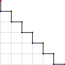
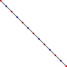
Figure 7. The doubling graph $D$, isomorphic to $\mathbb{Z}$, shown on the left in correspondence with two successive diagonals $S_{k}$, $S_{k+1}$ of $\mathbb{Z}^{2}$.

Recall the definition of the hard-core model as given in Section 1.2; a Gibbs distribution for the hard-core model on a graph with vertex set $W$ with activity $\lambda>0$ is a distribution on configurations $\eta\in\{0,1\}^{W}$ satisfying (1.2).

Consider the hard-core model on the doubling graph $D$ with vertex set $W=\mathbb{Z}$. This is a bipartite graph, with bipartition $W=W_{0}\cup W_{1}$ where $W_{0}$ and $W_{1}$ are the sets of even and odd integers respectively. We consider the following two update procedures for configurations on $\{0,1\}^{W}$. For an “odd” update, for each vertex $x\in W_{1}$ independently, resample $\eta(x)$ according to the values at its two neighbours, setting $\eta(x)=0$ with probability 1 if either of the neighbours takes value 1, and otherwise setting $\eta(x)=1$ with probability $1-p$. For an “even” update, do the same for vertices in $W_{0}$. Set $\lambda=1/p-1$, so that $1-p=\lambda/(1+\lambda)$. Since each of $W_{0}$ and $W_{1}$ is an independent set of $D$, any Gibbs distribution for the hard-core model with activity $\lambda$ is invariant under both of these update operations. (This is a version of Glauber dynamics).

Take some even $k\in\mathbb{Z}$. Suppose we start from a configuration on $\{0,1\}^{W}$, which, via the isomorphism (3.4) between $D$ and $D_{k}$ under which $W_{0}$ maps to $S_{k}$ and $W_{1}$ to $S_{k+1}$, corresponds to a configuration in $\{0,1\}^{S_{k}\cup S_{k+1}}$. Perform an odd update, resampling the sites of $W_{1}$, leading to a new configuration on $\{0,1\}^{W}$. Considering now (3.4) as an isomorphism between $D_{k}$ and $D_{k-1}$, which maps $W_{0}$ to $S_{k}$ and $W_{1}$ to $S_{k-1}$, the updated configuration on $\{0,1\}^{W}$ corresponds to a configuration in $\{0,1\}^{S_{k-1}\cup S_{k}}$, whose values at the sites in $S_{k}$ are left unchanged. We can interpret the update as generating a configuration on $S_{k-1}$ from a configuration on $S_{k}$. This procedure is identical to that which occurs in one iteration of the PCA $A_{p,0}$.

If we then perform an even update, resampling the sites of $W_{0}$, we can pass in the same way to a configuration on the sites of $S_{k-2}\cup S_{k-1}$, which corresponds to the next step of the PCA.

Continuing to perform odd and even updates alternately, we reproduce the evolution of the PCA. A Gibbs distribution on $D$ is characterized by its marginal on the vertices of one half of the bipartition, say $W_{0}$. Since the distribution is preserved by the updates, this distribution on $\{0,1\}^{W_{0}}$ is $2$-periodic for the PCA.

In fact, for any $\lambda$ there is a unique Gibbs distribution for the hard-core model on $\mathbb{Z}$. Since the hard-core interaction is homogeneous and nearest-neighbour, this Gibbs distribution is itself a stationary Markov chain indexed by $\mathbb{Z}$. Let $Q=Q_{p}$ be its transition matrix. Therefore, the marginal distributions on $W_{0}$ and $W_{1}$ are in fact equal to each other. Call this marginal distribution $\mu_{p}$. Then $\mu_{p}$ is the law of the stationary Markov chain with transition matrix $P=Q^{2}$. This $\mu_{p}$ is a stationary distribution for the PCA $A_{p,0}$, and the matrix $P$ is the one in (3.1). See Figure 8 for an illustration.

Figure 8. The Markovian distribution corresponding to a Gibbs measure for the hard-core model on the doubling graph $W$ yields a Markovian distribution $\mu_{p}$ on each of the two vertex classes $W_{0}$ and $W_{1}$. Since the Gibbs distribution is invariant under the update procedures, the distribution $\mu_{p}$ is invariant for the PCA.

Combining with monotonicity properties (of the sort written in Lemma 2.1(i)), one can use the uniqueness of the Gibbs measure on $\mathbb{Z}$ to conclude that $A_{p,0}$ indeed has a unique stationary distribution; we explain this in a more general setting in Section 3.3.

Before that, in the next section we will use the implication in the other direction to establish the result of Theorem 2; in situations where there exist multiple Gibbs distributions for the hard-core model, we can conclude that there are multiple periodic distributions for the corresponding PCA; then the PCA is non-ergodic, and draws occur with positive probability in the corresponding game.

3.2. General framework

Recall that in the setting of Theorem 2, we have a locally finite graph $G$ with vertex set $V$, along with a partition $(S_{k}:k\in\mathbb{Z})$ of $V$ and an integer $m\geq 2$, such that conditions (A1) and (A2) given in Section 1.2 hold.

We also defined $D_{k}$ be the graph with vertex set $S_{k}\cup\dots\cup S_{k+m-1}$, with an undirected edge $(x,y)$ whenever $(x,y)$ is a (directed) edge of $V$. For convenience we will also use $D_{k}$ to denote the vertex set $S_{k}\cup\dots\cup S_{k+m-1}$.

Lemma 3.1.

The graphs $D_{k}$ are isomorphic to each other for all $k\in\mathbb{Z}$.

Proof.

Consider the map $\chi_{k}$ defined on $D_{k}$ under which

$$\chi_{k}(x)=\begin{cases}x&\text{ if }x\in S_{k+1}\cup\dots\cup S_{k+m-1}\\ \phi(x)&\text{ if }x\in S_{k}\end{cases}.$$

From assumptions (A1) and (A2) above, $\chi_{k}$ is a graph isomorphism from $D_{k}$ to $D_{k+1}$. Hence indeed $D_{k}$ and $D_{k+1}$ are isomorphic, and so by induction any two $D_{k}$, $D_{k^{\prime}}$ are isomorphic. ∎

We then take $D$ to be a graph isomorphic to any $D_{k}$. (When $m=2$ we sometimes call $D$ the doubling graph). Note that $D$ is $m$-partite. Specifically, let us fix some isomorphism $f_{0}$ from $D_{0}$ to $D$, and let $W_{i}$ be the image of $S_{i}$ under $f_{0}$, for $i=0,\dots,m-1$. Then $(W_{0},\ldots,W_{m-1})$ is a partition of the vertices of $D$ into $m$ classes, and assumption (A1) guarantees that there are no edges within a class $W_{i}$.

It will be important that we can map both $D_{k}$ and $D_{k+1}$ to $D$ in such a way that the vertices common to $D_{k}$ and $D_{k+1}$ have the same image in both maps.

Lemma 3.2.

There exists a family of maps $(f_{k}:k\in\mathbb{Z})$ such that $f_{k}$ is a graph isomorphism from $D_{k}$ to $D$, and such that the following properties hold.

• For each $k$,

  $$f_{k}(x)=\begin{cases}f_{k+1}(x)&\text{ for }x\in D_{k}\cap D_{k+1}=S_{k+1}\cup\dots\cup S_{k+m-1}\\ f_{k+1}(\phi(x))&\text{ for }x\in S_{k}.\end{cases}$$

• For each $k$ and each $r\in\{k,k+1,\dots,k+m-1\}$, the image of $S_{r}$ under $f_{k}$ is $W_{r\operatorname{mod}m}$.

• Let $x\in S_{k}$ and $y\in D_{k}=S_{k}\cup\dots\cup S_{k+m-1}$. Then $y\in\operatorname{Out}(x)$ if and only if $f_{k}(y)$ is a neighbour of $f_{k}(x)$ in $D$.

Proof.

Let $f_{0}$ be the isomorphism from $D_{0}$ to $D$ described just above. Then we can compose $f$ with the isomorphisms $\chi_{k}$ defined in the proof of Lemma 3.1, by setting

$$f_{k}=\begin{cases}f_{0}\circ\chi_{-1}\circ\chi_{-2}\circ\dots\circ\chi_{k}&\text{ for }k<0\\ f_{0}\circ\chi_{0}^{-1}\circ\chi_{1}^{-1}\circ\dots\circ\chi_{k-1}^{-1}&\text{ for }k>0.\end{cases}$$

Then using assumption (A2), it is easy to check by induction upwards and downwards from $0$ that $f_{k}$ is an isomorphism from $D_{k}$ to $D$ satisfying the properties stated in (a) and (b), for each $k$.

Finally note that by (A1), if $x\in S_{k}$ then $\operatorname{Out}(x)\subseteq S_{k}\cup\dots\cup S_{k+m-1}$ while $\operatorname{In}(x)$ is disjoint from $S_{k}\cup\cdots\cup S_{k+m-1}$. By definition, the set of neighbours of $x$ in the graph $D_{k}$ is then $\operatorname{Out}(x)$. Then part (c) follows since $f_{k}$ is a graph isomorphism from $D_{k}$ to $D$. ∎

Given a hard-core configuration in $\{0,1\}^{D}$, we can consider Glauber update steps that resample the vertices of one of the vertex classes $W_{0}$, $W_{1},\dots,W_{m-1}$. To perform an update of the class $W_{i}$: for each $v\in W_{i}$ independently, let the new value at $v$ be 0 if any neighbour of $x$ has value 1, and otherwise let the new value at $v$ be 0 with probability $p=1/(1+\lambda)$ and 1 with probability $1-p=\lambda/(1+\lambda)$. If a distribution on $\{0,1\}^{D}$ is a Gibbs distribution for the hard-core model on $D$ with activity $\lambda=1/p-1$, then it is invariant under this update procedure for each $i=0,1,\dots,m-1$. (Again, this is a version of the Glauber dynamics for the hard-core model on $D$.)

Proof of Theorem 2.

We start by defining an analogue of the hard-core PCA $A_{p,0}$ in the general setting. As before, we have the recursion (2.1) for the outcome of the game started from $x\in V$, in terms of the outcomes started from the elements of $\operatorname{Out}(x)$ together with the information whether $x$ itself is a trap or open. (Recall that we treat the game from $x$ as a win if $x$ is a trap.)

As in previous sections we can specialize that recursion to configurations involving only the symbols $0=W$ and $1=L$. This gives the following recursion for a family of variables $(\gamma(x):x\in V)\in\{0,1\}^{V}$ (which we do not assume to be necessarily game outcomes):

(3.5) $$\text{$x$ a trap}\;\Rightarrow\;\gamma(x) =0;$$

$$\text{$x$ open}\;\Rightarrow\;\gamma(x) =\begin{cases}1&\text{if }\gamma(y)=0\text{ for all }y\in\operatorname{Out}(x)\\ 0&\text{if }\gamma(y)=1\text{ for some }y\in\operatorname{Out}(x).\end{cases}$$

If $x\in S_{k}$, then $\operatorname{Out}(x)\subset S_{k+1}\cup\dots\cup S_{k+m-1}$. Thus, the recursion (3.5) gives $(\gamma(x):x\in S_{k})$ in terms of $(\gamma(x):x\in S_{k+1}\cup\dots\cup S_{k+m-1})$ and the random percolation configuration of traps and open sites in $S_{k}$ (which we take as usual to be product measure with each site being a trap with probability $p$). This is analogous to the PCA $A_{p,0}$ considered earlier (although for $m>2$, a “state” of the PCA is now more complicated to describe).

Fix $K\in\mathbb{Z}$, and take some boundary condition $(\gamma(x):x\in S_{K}\cup\cdots\cup S_{K+m-1})$, which we allow to be be random, but which is independent of the percolation configuration in $\bigcup_{r<K}S_{r}$. Applying (3.5) repeatedly then generates an evolution $(\gamma(x):x\in S_{r})_{r\leq K+m-1}$.

We will couple this evolution with a process of configurations in $\{0,1\}^{D}$. For $k\leq K$ and $v\in D$, define $\sigma_{k}(v)=\gamma(f_{k}^{-1}(v))$. Then $\sigma_{k}\in\{0,1\}^{D}$ for each $k$. The idea is now to show that the transformation from $\sigma_{k+1}$ to $\sigma_{k}$ is identical to a hard-core update of the vertex class $W_{k\operatorname{mod}m}$, with randomness provided by the percolation configuration of open in $S_{k}$. Notice that $\sigma_{k+1}$ is a function of $(\gamma(x):x\in S_{k+1}\cup\dots\cup S_{k+m})$, while $\sigma_{k}$ is a function of $(\gamma(x):x\in S_{k}\cup\dots\cup S_{k+m-1})$.

If $v\in W_{i}$ where $i\neq k\operatorname{mod}m$, then by Lemma 3.2(a) and (b), $f_{k+1}^{-1}(v)=f_{k}^{-1}(v)\in S_{k+1}\cup\dots\cup S_{k+m-1}$. Thus $\sigma_{k+1}(v)=\sigma_{k}(v)$. So the only sites in $D$ which can change their value between the configuration $\sigma_{k+1}$ and the configuration $\sigma_{k}$ are those in $W_{k\operatorname{mod}m}$. Consider such a $v\in W_{k\operatorname{mod}m}$, and let $x=f^{-1}_{k}(v)$ so that $x\in S_{k}$ (by Lemma 3.2(b)) and $\sigma_{k}(v)=\gamma(x)$.

Translating (3.5) and using Lemma 3.2(c) gives that for $v\in W_{k\operatorname{mod}m}$:

(3.6) $$\text{$x$ a trap}\;\Rightarrow\;\sigma_{k}(v) =0;$$

$$\text{$x$ open}\;\Rightarrow\;\sigma_{k}(v) =\begin{cases}1&\text{if }\sigma_{k+1}(u)=0\text{ for all }u\sim v\\ 0&\text{if }\sigma_{k+1}(u)=1\text{ for some }u\sim v.\end{cases}$$

Each bit of randomness (the information about whether $x\in S_{k}$ is an open site or a trap) is used only once. Since each $x$ is a trap with probability $p$ independently, we have that the conditional distribution of $\sigma_{k}$ given $\sigma_{k+1},\sigma_{k+2},\dots,\sigma_{K}$ is precisely that obtained by performing a hard-core update of the vertex class $W_{k\operatorname{mod}m}$.

Now let $\mu$ be a Gibbs distribution for the hard-core model on $D$. By choosing the distribution of the boundary condition $(\gamma(x):x\in S_{K}\cup\cdots\cup S_{K+m-1})$ correspondingly, we can arrange that $\sigma_{K}$ has distribution $\mu$. But then since $\mu$ is invariant under the hard-core updates, $\sigma_{k}$ has distribution $\mu$ for all $k<K$ also.

So, suppose that there exist multiple Gibbs distributions, and let $\mu$ and $\nu$ be two of them. By alternating between $\mu$ and $\nu$, we can arrange a sequence indexed by $K$ of boundary conditions $(\gamma^{(K)}(x):x\in S_{K}\cup\cdots\cup S_{K+m-1})$ that induces a sequence of distributions of $\sigma^{(K)}_{0}$ having both $\mu$ and $\nu$ as limit points as $K\to\infty$. In particular, the configuration $\sigma^{(K)}_{0}$ does not converge almost surely as $K\to\infty$ (in the product topology). So the sequence of configurations $(\gamma^{(K)}(x):x\in S_{0}\cup\cdots\cup S_{m-1})$ does not converge almost surely.

Now we apply the same argument that we used for the second part of the proof of Proposition 2.2. If the game started from $x$ is not a draw, then one player has a strategy which guarantees a win in fewer than $N$ moves, where $N\in\mathbb{N}$ is an almost surely finite random variable which depends on the configuration. Then the values $\gamma^{(K)}(x)$ must agree for all large enough $K$. Hence if there is zero probability of a draw from each site, then the configuration $(\gamma^{(K)}(x):x\in S_{0}\cup\cdots\cup S_{m-1})$ converges almost surely as $K\to\infty$. By the argument in the previous paragraph, this contradicts the existence of multiple hard-core Gibbs distributions. ∎

3.3. Remarks on the converse direction of Theorem 2

We do not know whether the converse of Theorem 2 holds in general; that is, whether the uniqueness of the hard-core Gibbs distribution on $D$ implies that there are no draws for the game on $G$. However, for the case $m=2$ (when the graph $D$ is bipartite), it is indeed the case that this converse direction also holds.

This can be established using a relatively standard argument involving Gibbs measures. Let us outline the argument. Let $m=2$, and let $D$ have vertex set $W=W_{0}\cup W_{1}$ as above. Let us write $B$ for the operator which first does a hard-core update of the sites in $W_{0}$, and then a hard-core update of the sites in $W_{1}$.

We can define a partial order on configurations in $\{0,1\}^{W}$ by setting $\sigma\leq\widetilde{\sigma}$ if $\sigma(v)\leq\widetilde{\sigma}(v)$ for all $v\in W_{0}$ and $\sigma(v)\geq\widetilde{\sigma}(v)$ for all $v\in W_{1}$. Then the operator $B$ (acting on distributions on $\{0,1\}^{W}$) is monotonic; if $\mu\leq\nu$ in the sense of stochastic domination, then also $B\mu\leq B\nu$. (This is closely related to the property in Lemma 2.1(i).) Let us write $\sigma^{\max}$ for the maximal configuration (taking value $1$ on all sites of $W_{0}$ and $0$ on all sites of $W_{1}$) and $\sigma^{\min}$ for the minimal configuration.

Then a monotonicity argument similar to that in Proposition 2.1 and Proposition 2.2 establishes that the probability of a draw is $0$ precisely if there is a unique stationary distribution on $\{0,1\}^{W}$ for the operator $B$.

Suppose therefore that there is a unique Gibbs measure $\mu$ for the hard-core model on $D$. We wish to show that $\mu$ is the unique invariant distribution for the operator $B$.

Consider any increasing sequence of finite subsets of $W$, $\Lambda_{1}\subset\Lambda_{2}\subset\dots\subset\Lambda_{n}\subset\dots$, with $\bigcup\Lambda_{n}=W$. Let $\mu^{\max}_{k,n}$ be the distribution obtained by applying the hard-core update procedure $k$ times on the sites of $\Lambda_{n}$, with the values at sites of $\Lambda_{n}^{c}$ fixed, starting from the configuration $\sigma^{\max}$. Let $\mu^{{\min}}_{k,n}$ be the analogous distribution starting from $\sigma^{\min}$.

We have that $\mu^{\max}_{k,n}\downarrow\mu^{\max}_{n}$ and $\mu^{\min}_{k,n}\uparrow\mu^{\min}_{n}$ as $k\to\infty$, where $\mu^{\max}_{n}$ and $\mu^{\min}_{n}$ are the hard-core measures on the finite vertex set $\Lambda_{n}$ with maximal and minimal boundary conditions respectively.

Furthermore, $\mu^{\max}_{n}\to\mu$ and $\mu^{\min}_{n}\to\mu$ as $n\to\infty$ (since any limit point of a sequence of Gibbs measures on the subsets $\Lambda_{n}$ is a Gibbs measure on the entire vertex set $W$, and we assume that $\mu$ is the only such Gibbs measure on $W$).

But if $\nu$ is any measure on $\{0,1\}^{W}$, then from the monotonicity of $B$ we have that $\mu^{\min}_{k,n}\leq B^{k}\nu\leq\mu^{\max}_{k,n}$ for all $k$. In particular suppose that $\nu$ is invariant. Then $B^{k}\nu=\nu$ for all $k$. But then by taking $k$ and $n$ sufficiently large, we can sandwich $\nu$ between two measures which are as close to $\mu$ as desired. This gives that $\nu=\mu$, and so indeed $B$ has a unique stationary distribution. Hence the probability of a draw is $0$, as required.

If however $m>2$, the graph is no longer bipartite, and the monotonicity argument above no longer works. In particular, we cannot define a partial ordering on configurations in the same way. Such a partial ordering was already used in the proof of Proposition 2.1, and without monotonicity, it is no longer clear that uniqueness of the invariant distribution for the PCA-like evolution on $\{0,1\}^{W}$ implies that the game has probability $0$ of a draw. (Closely related examples in which ergodicity of a binary PCA does not imply ergodicity of its envelope PCA are noted in [BMM13].) Furthermore, without monotonicity we could no longer apply the argument above involving bounds in terms of Gibbs measures on finite subsets with maximal and minimal boundary conditions.

3.4. Example graphs with $d\geq 3$

We now give several examples of graphs $G$ to which one may hope to apply Theorem 2. (As we will see, the result can indeed be applied in some cases, but not in others.) We consider the vertex set $V=\mathbb{Z}^{d}$ (or subsets thereof), for various different choices of the set $\operatorname{Out}(x)$ of vertices to which the token can move from $x$. In each case, we consider the trapping game in which each site is a trap with probability $p$ and open with probability $1-p$. All our examples can be regarded as natural extensions of the original $\mathbb{Z}^{2}$ game, in the sense that they reduce to it when we set $d=2$.

Example 3.1.

Let $\operatorname{Out}(x)=\{x+e_{i}:1\leq i\leq d\}$. So $|\operatorname{Out}(x)|=d$. This is perhaps the most natural extension of all. However we cannot apply Theorem 2 because there is no choice of the automorphism $\phi$ for which assumption (A2) holds.

Example 3.2.

Let $\operatorname{Out}(x)=\{x\pm e_{i}+e_{d}:1\leq i\leq d-1\}$. This is the example already mentioned in Section 1.2. Here $|\operatorname{Out}(x)|=2(d-1)$. Since any step preserves parity, it is natural to restrict to the set of even sites $\mathbb{Z}^{d}_{\text{even}}:=\{x\in\mathbb{Z}^{d}:\sum x_{i}\text{ is even}\}$.

In two dimensions, the game is isomorphic to the original game on $\mathbb{Z}^{2}$. For general $d$, conditions (A1) and (A2) hold with $m=2$ if we set $S_{k}=\{x\in\mathbb{Z}^{d}_{\text{even}}:x_{d}=k\}$ and $\phi(x)=x+2e_{d}$.

To obtain the doubling graph, consider $D_{k}=S_{k}\cup S_{k+1}$ with an edge between $x\in S_{k}$ and $y\in S_{k+1}$ whenever $y\in\operatorname{Out}(x)$. This gives a graph isomorphic to the standard cubic lattice $\mathbb{Z}^{d-1}$ (for example, the map

$$(x_{1},\dots,x_{d-1},x_{d})\to(x_{1},\dots,x_{d-1})$$

gives a graph isomorphism from $D_{0}=S_{0}\cup S_{1}$ to $\mathbb{Z}^{d-1})$.

The graph is vertex-transitive. By Theorem 2, if there exist multiple Gibbs distributions for the hard-core model on $\mathbb{Z}^{d-1}$ with activity $\lambda$, then the percolation game on $G$ with $p=1/(1+\lambda)$ has positive probability of a draw from any vertex.

Example 3.3.

Now let $\operatorname{Out}(x)=\{x\pm e_{1}\pm e_{2}\dots\pm e_{d-1}+e_{d}\}$, so that $|\operatorname{Out}(x)|=2^{d-1}$. Each step changes the parity of every coordinate, so we restrict to the set $\mathbb{Z}^{d}_{\text{bcc}}=\{x\in\mathbb{Z}^{d}:x_{i}\equiv x_{j}\bmod 2\text{ for all }i,j\}$. Putting an edge between $x$ and $y$ whenever $y\in\operatorname{Out}(x)$, we obtain the body-centred cubic lattice in $d$ dimensions. This consists of two copies of $(2\mathbb{Z})^{d}$, each offset from the other by $(1,1,\dots,1)$, so that each point of one lies at the centre of a unit cube of the other; the edges are given by joining each point to the $2^{d}$ corners of the surrounding unit cube. See Figure 9 for an illustration.

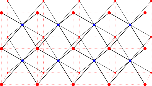
Figure 9. The three-dimensional body-centred cubic lattice (which is the doubling graph for the PCA associated to Example 3.3 when $d=4$). The two underlying copies of $\mathbb{Z}^{3}$ are shown with red and with blue vertices. The black lines are the edges of the body-centred cubic lattice, and the dotted red lines show the nearest-neighbour edges in the red copy of $\mathbb{Z}^{3}$.

Conditions (A1) and (A2) hold for $m=2$ with $S_{k}=\{x\in\mathbb{Z}^{d}_{\text{bcc}}:x_{d}=k\}$ and $\phi(x)=x+2e_{d}$. The doubling graph $D$ isomorphic to $D_{k}=S_{k}\cup S_{k+1}$ for each $k$ is now the body-centered cubic lattice in $d-1$ dimensions. The map $v(x)=(x_{1},x_{2},\dots,x_{d-1})$ from $\mathbb{Z}^{d}_{\text{bcc}}$ to $\mathbb{Z}^{d-1}_{\text{bcc}}$ restricts to an isomorphism between $D_{k}$ and $D$ for each $k$.

When $d=2$ or $d=3$ the graph $G$ is isomorphic to that in Example 3.2 above, but for $d\geq 4$ the graphs are different. Existence of multiple hard-core distributions on $\mathbb{Z}^{d-1}_{\text{bcc}}$ will imply existence of draws on $\mathbb{Z}^{d}_{\text{bcc}}$.

Example 3.4.

Let $\operatorname{Out}(x)=\{x+\sum_{i\in S}e_{i}:S\subset\{1,\dots,d\}\text{ with }1\leq|S|\leq d-1\}$. So a move of the game corresponds to incrementing at least one, but not all, of the coordinates by one. Then $|\operatorname{Out}(x)|=2^{d}-2$.

Conditions (A1) and (A2) hold with $m=d$ if we set $S_{k}=\{x:\sum x_{i}=k\}$ and $\phi(x)=x+e_{1}+e_{2}+\dots+e_{d}$. For $d=2$ the game is the same as ever. For $d>2$ there are some new features. For the first time we have $m>2$, and the graph $G$ is not bipartite; from a given starting vertex, there are vertices that can be reached when it is either player’s turn. The graph $D$ is $(d-1)$-dimensional and $d$-partite. For $d=3$, it corresponds to the triangular lattice. For example, the map

(3.7) $$(x_{1},x_{2},x_{3})\to x_{1}(1,0)+x_{2}\bigl{(}-\tfrac{1}{2},\tfrac{\sqrt{3}}{2}\bigr{)}+x_{3}\bigl{(}-\tfrac{1}{2},-\tfrac{\sqrt{3}}{2}\bigr{)}$$

is an isomorphism from $D_{k}=S_{k}\cup\dots\cup S_{k+m-1}$ to the triangular lattice for each $k$.

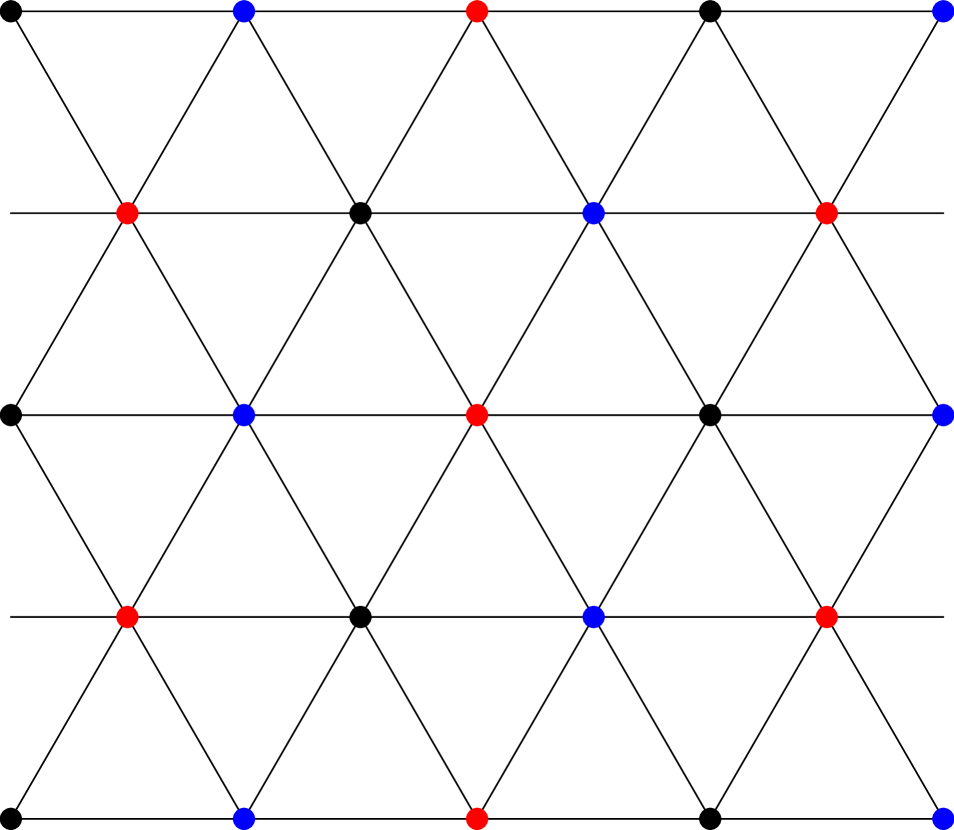
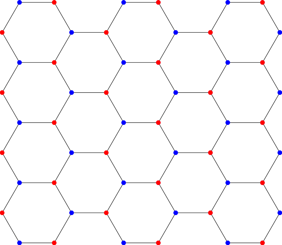
Figure 10. Triangular lattice and hexagonal lattice.

Example 3.5.

Fix $r$ with $1\leq r\leq d$, and now restrict to sites $x\in\mathbb{Z}^{d}$ such that $\sum x_{i}\equiv 0\text{ or }r\bmod d$. For $x$ with $\sum x_{i}\equiv 0\bmod d$, let $\operatorname{Out}(x)=\{x+\sum_{i\in S}e_{i},\text{ for any }S\subset\{1,\dots,d\}\text{ with }|S|=r\}$. Meanwhile, for $x$ with $\sum x_{i}\equiv r\bmod d$, let $\operatorname{Out}(x)=\{x+\sum_{i\in S}e_{i},\text{ for any }S\subset\{1,\dots,d\}\text{ with }|S|=d-r\}$.

Now $|\operatorname{Out}(x)|=\left(\begin{smallmatrix}d\\ r\end{smallmatrix}\right)$ for all $x$. Replacing $r$ by $d-r$ gives an isomorphic graph, so we may assume $1\leq r\leq d/2$. Then conditions (A1) and (A2) hold with $m=2$, with $\phi(x)=x+\sum_{i=1}^{d}e_{i}$, and with $S_{k}=\{x:\sum x_{i}=dk/2\}$ for even $k$ and $S_{k}=\{x:\sum x_{i}=d(k-1)/2+r\}$ for odd $k$.

For $d=2$ (and hence $r=1$) the game is the familiar two-dimensional game. For $d=3$ and $r=1$, we get $|\operatorname{Out}(x)|=3$ and the doubling graph $D$ is the two-dimensional hexagonal lattice; this is the image of $\{x\in\mathbb{Z}^{d}:\sum x_{i}\equiv 0\text{ or }1\bmod 3\}$, with edges between $x$ and $y$ where $y\in\operatorname{Out}(x)$, under the map (3.7) above.

For $d=4$ and $r=2$, the graph $G$ is isomorphic to the $d=4$ case of Example 3.2 above, and so $D$ is the standard cubic lattice $\mathbb{Z}^{3}$. For $d=4$ and $r=1$, we have $|\operatorname{Out}(x)|=4$, and $D$ is the so-called diamond cubic graph (see for example Section 6.4 of [CS99]). This graph may, for example, be represented as

$$\bigl{\{}y\in\mathbb{Z}^{3}:y_{1}\equiv y_{2}\equiv y_{3}\bmod 2\text{ and }y_{1}+y_{2}+y_{3}\equiv 0\text{ or }1\bmod 4\bigr{\}},$$

with edges between nearest neighbours (which are at distance $\sqrt{3}/4$). This is the image of $\{x\in\mathbb{Z}^{d}:\sum x_{i}\equiv 0\text{ or }1\bmod 3\}$, with edges between $x$ and $y$ where $y\in\operatorname{Out}(x)$, under the map

$$\begin{pmatrix}y_{1}\\ y_{2}\\ y_{3}\end{pmatrix}=\begin{pmatrix}\phantom{-}x_{1}-x_{2}-x_{3}+x_{4}\\ -x_{1}+x_{2}-x_{3}+x_{4}\\ \phantom{-}x_{1}+x_{2}-x_{3}-x_{4}\end{pmatrix}$$

(see [NS08]). See Figure 11 for an illustration.

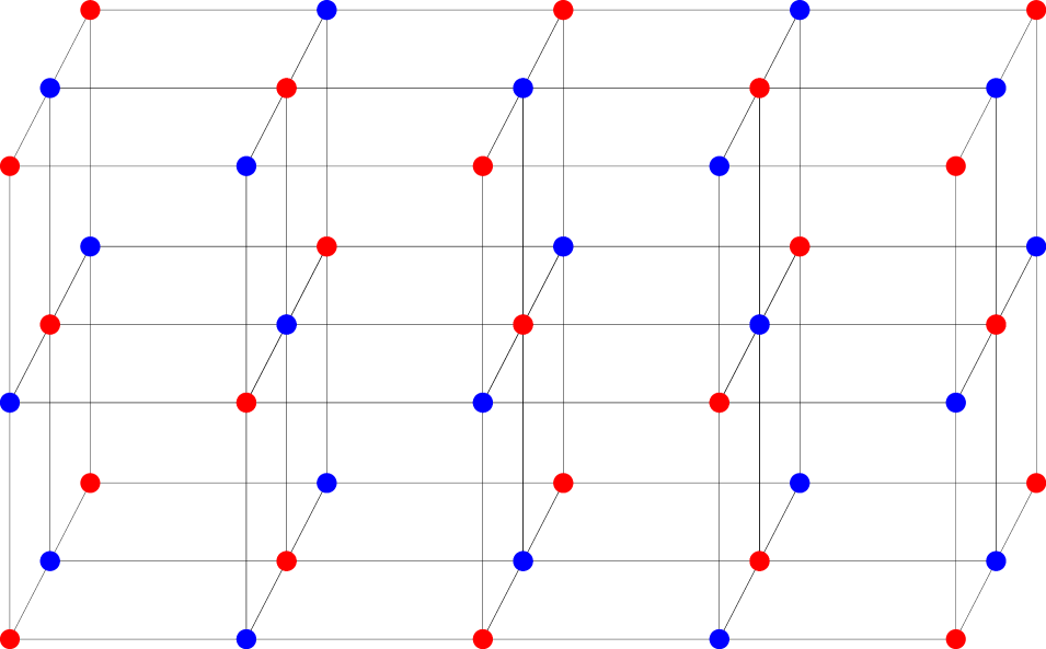
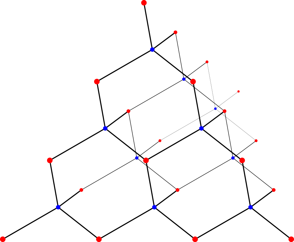
Figure 11. The cubic lattice and the diamond cubic graph.

Theorem 3.

There is positive probability of a draw from every vertex for sufficiently small $p$ in the following cases: Example 3.2 for all $d\geq 3$; Example 3.3 for $d=3$ and $d=4$; Example 3.4 for $d=3$; and Example 3.5 for $d=3$ (with $r=1$) and $d=4$ (with $r=1$ or $r=2$).

Proof.

In the cases listed, it is known that there exist multiple Gibbs distributions for the hard-core model on the associated graph $D$ when the activity parameter $\lambda$ is sufficiently high. For the standard cubic lattice in any dimension greater than 1, the result goes back to Dobrushin [Dob65]. Other models in two and three dimensions were covered by Heilmann [Hei74] and Runnels [Run75], including the triangular and hexagonal lattices in two dimensions and the body-centered cubic lattice and the diamond cubic graph in three dimensions.

Theorem 2 shows that there is positive probability of a draw for small enough $p$ from some vertex, and since all the graphs $G$ are vertex-transitive, the conclusion holds for every vertex. ∎

It is expected that in fact the hard-core model on $D$ has multiple Gibbs distributions for $\lambda$ sufficiently large in all of Examples 3.2–3.5 whenever $d\geq 3$ (so that $D$ has dimension at least $2$). This could likely be proved by Peierls contour arguments, although this requires a suitable definition of a contour, which is typically graph-dependent, and less straightforward than in other settings such as the Ising model. Via Theorem 2, such non-uniqueness would imply existence of draws for the corresponding graphs $G$.

We emphasize again that there is a more fundamental obstacle to proving existence of draws for the standard oriented lattice $\mathbb{Z}^{d}$ of Example 3.1, in that our condition (A2) does not hold here.

3.5. Extending the hard-core correspondence

Various further extensions can be made while still preserving the correspondence to the hard-core model. For example, in the class of models considered in Theorem 2, we can augment the set of allowable moves from site $x$ to include the point $\phi(x)$ itself.

Specifically, replace (A1) and (A2) by the following assumptions:

• For all $x\in S_{k}$, $\operatorname{Out}(x)\subset S_{k+1}\cup\dots\cup S_{k+m-1}\cup\{\phi(x)\}$.

• There is a graph automorphism $\phi$ of $G$ that maps $S_{k}$ to $S_{k+m}$ for every $k$, such that $\phi(x)\in\operatorname{Out}(x)$ for all $x$, and such that $\operatorname{Out}(x)\setminus\{\phi(x)\}=\operatorname{In}(\phi(x))\setminus x$.

Define $D$ as before; $D$ is a graph isomorphic to any $D_{k}$, where $D_{k}$ is the graph with vertex set $S_{k}\cup\dots\cup S_{k+m-1}$ and an undirected edge $(x,y)$ whenever $(x,y)$ is a directed edge of $V$. Note now an edge $(x,\phi(x))$ in $G$ does not give a corresponding edge in $D$.

Proposition 3.1.

Suppose that the graph $G$ satisfies (A$1^{\prime}$) and (A$2^{\prime}$). If there are multiple Gibbs distributions for the hard-core model on $D$ with activity $\lambda<1$. then the percolation game on $G$ with $p=1-\lambda$ has positive probability of a draw from some vertex.

The method of proof is a slight variation on that of Theorem 2, which we indicate briefly. To reflect the presence of the edge $(x,\phi(x))$, we change the hard-core update procedure. When we perform an update of the vertex class $W_{i}$, we now add that any vertex $v\in W_{i}$ which is in state 1 before the update must move to state 0 after the update; otherwise the update at $v$ proceeds as before.

Again one can show that hard-core Gibbs distributions are stationarity under such updates, but now with the activity parameter $\lambda$ equal to $1-p$ rather than $1/p-1$ as previously. (To verify the stationarity, one can start by checking the detailed balance condition for an update at a single site; then if the distribution is stationary for the update at any single site, it is also invariant under simultaneous updates at any set of non-neighbouring sites.)

Note that now when $p\to 0$, we have $\lambda\to 1$ rather than $\lambda\to\infty$. Hence to show existence of draws for some $p$, we need multiplicity of Gibbs distributions for some $\lambda<1$. For the case of the standard cubic lattice, Galvin and Kahn [GK04] show that this holds for sufficiently high dimension, so that we can deduce the existence of draws for the variant of Example 3.2 in which $\operatorname{Out}(x)=\{x\pm e_{i}+e_{d}:1\leq i\leq d-1\}\cup\{x+e_{d}\}$, when $d$ is sufficiently large.

4. Open questions

4.1. The trapping game on the oriented cubic lattice

For the trapping game on $\mathbb{Z}^{d}$ (where the allowed moves from site $x$ are to any open site $x+e_{i}$ for $1\leq i\leq d$), do there exist any $p\in(0,1)$ and $d\geq 3$ for which draws occur with positive probability?

4.2. Percolation games in higher dimensions

Demonstrate positive probability of draws for percolation games with some $q>0$ on a natural class of lattices in dimension $d\geq 3$.

4.3. Monotonicity and phase transition

Consider settings where draws are known to occur – for example, the trapping game on the even sublattice of $\mathbb{Z}^{d}$ with $d\geq 3$ and moves allowed from $x$ to any open $x+e_{d}\pm e_{i}$ for $1\leq i\leq d-1$. Is the probability of a draw starting from the origin non-increasing in the density $p$ of traps? Or, at least, is the set of $p$ that have positive draw probability a single interval containing $0$ (so that there is a single critical point at the upper end of the interval)? If so, what happens at the critical point? In the light of the connection to the hard-core model, such questions are probably difficult – it is unknown, for example, whether the hard-core model on $\mathbb{Z}^{d}$ has a single critical point for uniqueness of Gibbs distributions (see e.g. [BGRT13] for discussion and recent bounds).

4.4. Converse statement of Theorem 2

As discussed in Section 3.3, the converse statement of Theorem 2 holds when $m=2$; that is, when we have a bipartite “doubling graph” $D$, the uniqueness of the hard-core Gibbs measure on $D$ is equivalent to zero probability of draws in the trapping game. Is this true also for $m>2$?

4.5. Computation of winning probabilities

Can one compute exact winning probabilties for games other than in the case of the trapping game on $\mathbb{Z}^{2}$ (see (1.1))? For example, as mentioned in the introduction, such questions for the more general percolation game on $\mathbb{Z}^{2}$ are related to the computation of generating functions for directed animals, enumerated according to their area and perimeter.

4.6. Misère games

In the target game (i.e. the percolation game with $p=0$ and $q>0$) the first player to move to a marked site (i.e. a target) wins. This can be seen as a misère version of the trapping game (i.e. the percolation game with $q=0$ and $p>0$), where the first player to move to a marked site (i.e. a trap) loses. There are also other natural misère variants of the trapping game. For example, suppose that each site is marked with probability $p$ and unmarked with probability $1-p$, and that moves are allowed from $x\in\mathbb{Z}^{2}$ only to an unmarked site in $\{x+e_{1},x+e_{2}\}$, but now declare that if both these sites are marked, then the player whose turn it is to move wins. Does this game have zero probability of a draw for all $p$? Here we don’t know of any useful correspondence to a PCA with alphabet $\{0,1\}$.

4.7. Elementary probabilistic cellular automata

Is every elementary PCA (i.e. one with $2$ states and a size-$2$ neighhborhood) on $\mathbb{Z}$ with positive rates ergodic? Can our weighting approach be extended to prove ergodicity for other PCA in this class?

4.8. Undirected lattices

The following game is considered in [BHMW16]. Each site of $\mathbb{Z}^{d}$ is independently a trap with probability $p$, and two players alternately move a token. From an open site $x$, a move is permitted to any open nearest neighbour $x\pm e_{i}$ provided it has not been visited previously. A player who cannot move loses. This game is closely related to maximum matchings, and this is used in [BHMW16] to derive results for biased variants in which odd and even sites have different percolation parameters. However, for the unbiased version described above it is unknown whether there exist any $p>0$ and $d\geq 2$ for which draws occur with positive probability. One can also extend the model to include targets as well as traps.

References

- [BBJW10] Paul Balister, Béla Bollobás, J. Robert Johnson, and Mark Walters. Random majority percolation. Random Structures Algorithms, 36(3):315–340, 2010.
- [BGM69] J. K. Beljaev, J. I. Gromak, and V. A. Malyšev. Invariant random Boolean fields. Mat. Zametki, 6:555–566, 1969.
- [BGRT13] Antonio Blanca, David Galvin, Dana Randall, and Prasad Tetali. Phase coexistence and slow mixing for the hard-core model on . In Approximation, Randomization, and Combinatorial Optimization. Algorithms and Techniques, pages 379–394. Springer, 2013.
- [BHMW16] Riddhipratim Basu, Alexander E. Holroyd, James B. Martin, and Johan Wästlund. Trapping games on random boards. Ann. Appl. Probab., 26(6):3727–3753, 2016.
- [BM98] Mireille Bousquet-Mélou. New enumerative results on two-dimensional directed animals. In Proceedings of the 7th Conference on Formal Power Series and Algebraic Combinatorics (Noisy-le-Grand, 1995), volume 180 of Discrete Math., pages 73–106, 1998.
- [BMM13] Ana Bušić, Jean Mairesse, and Irène Marcovici. Probabilistic cellular automata, invariant measures, and perfect sampling. Advances in Applied Probability, 45(4):960–980, 2013.
- [Con01] J. H. Conway. On numbers and games. A K Peters, Ltd., Natick, MA, second edition, 2001.
- [CS99] J. H. Conway and N. J. A. Sloane. Sphere packings, lattices and groups, volume 290 of Grundlehren der Mathematischen Wissenschaften [Fundamental Principles of Mathematical Sciences]. Springer-Verlag, New York, 3rd edition, 1999.
- [Dha83] Deepak Dhar. Exact solution of a directed-site animals-enumeration problem in three dimensions. Phys. Rev. Lett., 51(10):853–856, 1983.
- [Dob65] R. L. Dobrushin. Existence of a phase transition in the two-dimensional and three-dimensional Ising models. Soviet Physics Dokl., 10:111–113, 1965.
- [Elo96] Kari Eloranta. Golden Mean Subshift Revised. Research reports, Helsinki University of Technology, Institute of Mathematics. 1996.
- [Gác01] Peter Gács. Reliable cellular automata with self-organization. J. Statist. Phys., 103(1-2):45–267, 2001.
- [GH15] Janko Gravner and Alexander E. Holroyd. Percolation and disorder-resistance in cellular automata. Ann. Probab., 43(4):1731–1776, 2015.
- [GK04] David Galvin and Jeff Kahn. On phase transition in the hard-core model on . Combin. Probab. Comput., 13(2):137–164, 2004.
- [Gra01] Lawrence F. Gray. A reader’s guide to P. Gács’s “positive rates” paper. J. Statist. Phys., 103(1-2):1–44, 2001.
- [Hei74] Ole J. Heilmann. The use of reflection as symmetry operation in connection with Peierls’ argument. Comm. Math. Phys., 36:91–114, 1974.
- [HM] Alexander E. Holroyd and James B. Martin. Galton-Watson games. In preparation.
- [KV80] O. Kozlov and N. Vasilyev. Reversible Markov chains with local interaction. In Multicomponent random systems, volume 6 of Adv. Probab. Related Topics, pages 451–469. Dekker, New York, 1980.
- [LBM07] Yvan Le Borgne and Jean-François Marckert. Directed animals and gas models revisited. Electron. J. Combin., 14(1):71, 36 pp. (electronic), 2007.
- [MM14a] Jean Mairesse and Irène Marcovici. Around probabilistic cellular automata. Theoretical Computer Science, 559(0):42–72, 2014. Non-uniform Cellular Automata.
- [MM14b] Jean Mairesse and Irène Marcovici. Probabilistic cellular automata and random fields with i.i.d. directions. Ann. Inst. Henri Poincaré Probab. Stat., 50(2):455–475, 2014.
- [MM17] Jean Mairesse and Irène Marcovici. Uniform sampling of subshifts of finite type on grids and trees. Internat. J. Found. Comput. Sci., 28(3):263–287, 2017.
- [NS08] Benedek Nagy and Robin Strand. A connection betwen and generalized triangular grids. In ISVC 2008, volume 3539 of Lecture Notes in Computer Science, pages 1157–1166. Springer, Heidelberg, 2008.
- [Run75] L. K. Runnels. Phase transitions of hard sphere lattice gases. Comm. Math. Phys., 40:37–48, 1975.
- [TVS+90] A. L. Toom, N. B. Vasilyev, O. N. Stavskaya, L. G. Mityushin, G. L. Kurdyumov, and S. A. Pirogov. Discrete local Markov systems. In R. L. Dobrushin, V. I. Kryukov, and A. L. Toom, editors, Stochastic cellular systems: ergodicity, memory, morphogenesis, Nonlinear science, pages 1–175. Manchester University Press, 1990.
- [Vas78] N. B. Vasilyev. Bernoulli and Markov stationary measures in discrete local interactions. In Developments in statistics, Vol. 1, pages 99–112. Academic Press, New York, 1978.