Validity of the ICFT $R$-matrix method: Be-like Al ⁹⁺ a case study

Abstract

We have carried-out 98-level configuration-interaction / close-coupling (CI/CC) intermediate coupling frame transformation (ICFT) and Breit–Pauli $R$-matrix calculations for the electron-impact excitation of Be-like Al ⁹⁺. The close agreement that we find between the two sets of effective collision strengths demonstrates the continued robustness of the ICFT method. On the other hand, a comparison of this data with previous 238-level CI/CC ICFT effective collision strengths shows that the results for excitation up to $n=4$ levels are systematically and increasingly underestimated over a wide range of temperatures by $R$-matrix calculations whose close-coupling expansion extends only to $n=4$ (98-levels).

Thus, we find to be false a recent conjecture that the ICFT approach may not be completely robust. The conjecture was based upon a comparison of 98-level CI/CC Dirac $R$-matrix effective collision strengths for Al ⁹⁺ with those from the 238-level CI/CC ICFT $R$-matrix calculations. The disagreement found recently is due to a lack of convergence of the close-coupling expansion in the 98-level CI/CC Dirac work. The earlier 238-level CI/CC ICFT work has a superior target to the 98-level CI/CC Dirac one and provides more accurate atomic data.

Similar considerations need to be made for other Be-like ions and for other sequences.

1 Introduction

Electron-impact excitation is the dominant process for populating the radiating states of ions whose emission lines form the basis for the spectroscopic diagnostic modelling of non-equilibrium astrophysical and laboratory plasmas. As such, a great deal of effort over many years has gone in to calculating a large amount of collision data, which is incorporated into databases and modelling suites such as CHIANTI and OPEN-ADAS. The pre-eminent methodology used is the $R$-matrix one. However, there are many variations on this theme.

The intermediate coupling frame transformation (ICFT) $R$-matrix method is an approximation to the Breit–Pauli $R$-matrix method (BPRM) which neglects the spin–orbit interaction between the colliding electron and the ion. Thus, it is physically well motivated. There is a good deal of literature which verifies the accuracy of the ICFT approach: the original comparisons of the results of ICFT and Breit–Pauli $R$-matrix calculations by Griffin et al. (1998, 1999) on $\mathrm{Mg}$-like ions and Badnell & Griffin (1999) on $\mathrm{Ni}^{4+}$; more recent ones by Liang & Badnell (2010) comparing ICFT $R$-matrix and Dirac Atomic $R$-matrix Code (DARC) calculations for $\mathrm{Ne}$-like $\mathrm{Fe}^{16+}$ and $\mathrm{Kr}^{26+}$, Liang et al. (2009) on ICFT with Breit–Pauli and DARC for $\mathrm{Na}$-like $\mathrm{Fe}^{15+}$; and most recently Badnell & Ballance (2014) compared the results of ICFT, BPRM and DARC calculations for $\mathrm{Fe}^{2+}$. The differences observed between ICFT and other $R$-matrix results are all well within the uncertainties to be expected due to the use of different configuration interaction and close-coupling expansions and resonance resolution. Indeed, the Badnell & Ballance (2014) work on $\mathrm{Fe}^{2+}$ used identical atomic structures and close-coupling expansions for the ICFT and Breit–Pauli $R$-matrix calculations and found excellent agreement, better than $5\%$. Their DARC calculations out of necessity used a somewhat different atomic structure, and the low-level structure of $\mathrm{Fe}^{2+}$ is challenging, but still gave agreement to within $\sim 20\%$ at $10^{4}\,\mathrm{K}$.

Extensive calculations have been carried-out applying the ICFT $R$-matrix method to whole isoelectronic sequences (for elements, typically, up to $\mathrm{Zn}$), the most recent ones being $\mathrm{Mg}$-like (Fernández-Menchero et al. 2014b), $\mathrm{Be}$-like (Fernández-Menchero et al. 2014a) and $\mathrm{B}$-like (Liang et al. 2012) — this last paper contains references to earlier sequences.

Thus it is both surprising and of great concern to find a work which counters this trend: Aggarwal & Keenan (2015a) made a comparison of the results of a 98-level DARC calculation on $\mathrm{Be}$-like Al ⁹⁺ (Aggarwal & Keenan 2014c) with a 238-level ICFT $R$-matrix one (Fernández-Menchero et al. 2014a). Aggarwal & Keenan (2015a) found that the effective collision strengths obtained from the 238-level ICFT $R$-matrix calculation were significantly larger than the DARC ones in many instances and they suggested that the results of Fernández-Menchero et al. (2014a) were less reliable, querying the ICFT method, resonance resolution and its high energy / temperature behaviour.

In addition, Aggarwal & Keenan (2015a) alighted on the recent paper by Storey et al. (2014) which reported a problem in the outer-region ICFT calculation of $\mathrm{O}^{2+}$, when compared to a full Breit–Pauli calculation, and suggested that this could be the main cause of the discrepancies for Al ⁹⁺. However, Storey et al. (2014) noted that such an issue only arises when resonance effective quantum numbers become small. The problem is peculiar to low-charge ions such as $\mathrm{O}^{2+}$ and unusually small $R$-matrix box sizes. Storey et al. (2014) focused on providing a solution to their problem at hand. We note that the problem does not arise in the first place if the $R$-matrix box size is increased (beyond its default in their case) to encompass a spectroscopic $n=3$ orbital, say. This is why the issue had not arisen before: all previous calculations (including Fernández-Menchero et al. (2014a)) used larger, often much larger, box sizes. The problem noted by Storey et al. (2014) is not relevant in general. Aggarwal & Keenan (2015a) noted a similar trend for other ions of the Be-like sequence $\mathrm{Cl}^{13+}$, $\mathrm{K}^{15+}$, $\mathrm{Ge}^{28+}$ (Aggarwal & Keenan 2014a) and $\mathrm{Ti}^{18+}$ (Aggarwal & Keenan 2012).

Where does that leave us with regard to the discrepancies noted by Aggarwal & Keenan (2015a)? The concern of Aggarwal & Keenan (2015a) was the disagreement between $R$-matrix calculations of (apparent) comparable complexity. However, the works of Aggarwal & Keenan (2014c) and Fernández-Menchero et al. (2014a) are not of comparable complexity. We show here that the much larger close-coupling expansion used by (Fernández-Menchero et al. 2014a) (238 vs 98 levels) gives rise to a systematic enhancement of effective collision strengths over a wide range of temperatures, which increases as one excites higher-and-higher levels.

In addition, we analyze the uncertainty in the effective collision strengths due to the incompleteness of the configuration interaction expansion, the validity of the ICFT vs Breit–Pauli method, viz. the neglect of the spin–orbit interaction of the colliding electron, and the effect of resonance resolution and position on low temperature effective collision strengths.

The paper is organized as follows. In section 2 we describe the methodology we used for the different calculations we have performed. In section 3 we discuss the atomic structure of Al ⁹⁺ and present results for energies, line strengths and infinite energy plane wave Born collision strengths. In section 4 we compare and contrast effective collision strengths. In section 5 we present our main conclusions. Atomic units are used unless otherwise specified.

2 Methodology

In the following sections we compare the results of the 238-level configuration-interaction / close-coupling (CI/CC) ICFT $R$-matrix calculation by Fernández-Menchero et al. (2014a) for Al ⁹⁺ with the results of new ICFT and Breit–Pauli 98-level CI/CC $R$-matrix calculations — the latter being the same sized CI & CC expansions that were used by Aggarwal & Keenan (2012, 2014a, 2014c). Where possible (meaningful), our new 98-level CC calculations follow the same prescription as Fernández-Menchero et al. (2014a) e.g. with respect to angular momentum and energy specification.

The target description uses the autostructure program (Badnell 2011). Fernández-Menchero et al. (2014a) included all of the configurations $\mathrm{1s^{2}\,\{2s^{2},2s2p,2p^{2}\}}$ and $\mathrm{1s^{2}\,\{2s,2p\}}\,nl$ with $n=3-7$ and $l=\mathrm{s,p,d,f,g}$ for $n=3-5$ and $l=\mathrm{s,p,d}$ for $n=6,7$, which makes a total of 238 levels. In the present work, we restrict ourselves to $n=4$ (with $l=\mathrm{s,p,d,f}$) which gives a total of 98 levels. The Thomas–Fermi potential scaling parameters, $\lambda_{nl}$, for the atomic structure calculation with the CI basis set of 98 levels are given in Table 1, those for the CI calculation with 238 levels are given in Fernández-Menchero et al. (2014a). The $\lambda_{nl}$ parameters for the 98-level CI calculation were obtained in the same way as the ones for the 238-level calculation (Fernández-Menchero et al. 2014a): by minimizing the equally-weighted sum of all $LS$-coupling term energies.

Table 1: Scaling parameters $(\lambda_{nl})$ used in the 98-level CI structure calculation.

Orbital	$\lambda_{nl}$
1s	1.57175
2s	1.29675
2p	1.17081
3s	1.29004
3p	1.15958
3d	1.29791
4s	1.29797
4p	1.15413
4d	1.30212
4f	1.50916

For the collision calculations we use the inner-region $R$-matrix programs of Hummer et al. (1993); Berrington et al. (1995) and the outer-region stgf program of Berrington et al. (1987); Badnell (1999) plus the ICFT one of Griffin et al. (1998). We will compare the results of ICFT and Breit–Pauli $R$-matrix methods to treat relativistic effects in the scattering problem. Both can use the exact same Breit–Pauli atomic structure. This is important as it enables us to isolate differences due solely to the differing treatment of relativistic effects in the scattering. We note that Berrington et al. (2005) have shown that the Breit–Pauli $R$-matrix method gives essentially the same results as the Dirac one for $Z\lesssim 30$.

The ICFT $R$-matrix method first carries-out an $LS$-coupling close-coupling calculation for the CI target described above and it includes the mass-velocity and Darwin one-body relativistic operators. The $LS$-coupling reactance $K$-matrices are first recoupled to $jK$-coupling and then transformed to intermediate coupling using the term coupling coefficients (Hummer et al. 1993) for the Breit–Pauli target. This imposes the exact same atomic structure on the ICFT $K$-matrices as a Breit–Pauli one which uses the same CI expansion and radial orbitals. In particular, the fine-structure levels within a term are non-degenerate in the final scattering calculation. This method is the one which was used by Fernández-Menchero et al. (2014a).

The second method which we use is the Breit–Pauli (BP) one. In this method the close-coupling expansion is made in intermediate coupling as well, in addition to the target CI, i.e. the one-body effective (nuclear plus Blume & Watson) spin–orbit operator is included in the $(N+1)$-electron Hamiltonian. The Breit–Pauli formalism increases considerably the size of the Hamiltonian matrix, which makes it impractical to use this method for 238 CC levels.

The essential physical difference between the ICFT and Breit-Pauli $R$-matrix methods is the neglect by the former of the effective spin–orbit interaction between the colliding electron and the ion. The practical benefit of the ICFT method over the Breit–Pauli one is the diagonalization of much smaller $(N+1)$-electron Hamiltonian matrices and a much smaller set of coupled scattering equations to be solved in the outer-region by stgf.

3 Structure

Table 2: $\mathrm{Al}^{9+}$ target levels. Key: $i$: level index; Conf.: configuration; Level: level IC designation (largest weight); $E_{\mathrm{NIST}}$: observed energy from the NIST database (Martin & Zalubas 1979); $E_{98}$: calculated energy with 98-level CI expansion; $E_{238}$: calculated energy with 238-level CI expansion (see text); %: percentage difference between theoretical and NIST data. All energies are in $\mathrm{cm}^{-1}$.

$i$	Conf.	Level	$E_{\mathrm{NIST}}$	$E_{98}$ (	%)	$E_{238}$ (	%)	$i$	Conf.	Level	$E_{\mathrm{NIST}}$	$E_{98}$ (	%)	$E_{238}$ (	%)
1	$\mathrm{2s^{2}}$	$\mathrm{{}^{1}S_{0}}$	$0.$	$0.$ (	$0$)	$0.$ (	$0$)	50	$\mathrm{2s\,4p}$	$\mathrm{{}^{3}P_{1}^{o}}$	$-$	$2504724.$ (	$-$)	$2500556.$ (	$-$)
2	$\mathrm{2s\,2p}$	$\mathrm{{}^{3}P_{0}^{o}}$	$155148.$	$155722.$ (	$0.4$)	$155539.$ (	$0.3$)	51	$\mathrm{2s\,4p}$	$\mathrm{{}^{3}P_{2}^{o}}$	$-$	$2505125.$ (	$-$)	$2500975.$ (	$-$)
3	$\mathrm{2s\,2p}$	$\mathrm{{}^{3}P_{1}^{o}}$	$156798.$	$157487.$ (	$0.4$)	$157404.$ (	$0.4$)	52	$\mathrm{2s\,4p}$	$\mathrm{{}^{1}P_{1}^{o}}$	$-$	$2508073.$ (	$-$)	$2503514.$ (	$-$)
4	$\mathrm{2s\,2p}$	$\mathrm{{}^{3}P_{2}^{o}}$	$160429.$	$161146.$ (	$0.4$)	$161278.$ (	$0.5$)	53	$\mathrm{2s\,4d}$	$\mathrm{{}^{3}D_{1}}$	$-$	$2520502.$ (	$-$)	$2516248.$ (	$-$)
5	$\mathrm{2s\,2p}$	$\mathrm{{}^{1}P_{1}^{o}}$	$300490.$	$309273.$ (	$2.9$)	$307209.$ (	$2.2$)	54	$\mathrm{2s\,4d}$	$\mathrm{{}^{3}D_{2}}$	$-$	$2520573.$ (	$-$)	$2516321.$ (	$-$)
6	$\mathrm{2p^{2}}$	$\mathrm{{}^{3}P_{0}}$	$404574.$	$408026.$ (	$0.9$)	$407826.$ (	$0.8$)	55	$\mathrm{2s\,4d}$	$\mathrm{{}^{3}D_{3}}$	$-$	$2520682.$ (	$-$)	$2516434.$ (	$-$)
7	$\mathrm{2p^{2}}$	$\mathrm{{}^{3}P_{1}}$	$406517.$	$409969.$ (	$0.8$)	$409888.$ (	$0.8$)	56	$\mathrm{2s\,4d}$	$\mathrm{{}^{1}D_{2}}$	$2527560.$	$2530218.$ (	$0.1$)	$2525880.$ (	$-0.1$)
8	$\mathrm{2p^{2}}$	$\mathrm{{}^{3}P_{2}}$	$409690.$	$413420.$ (	$0.9$)	$413526.$ (	$0.9$)	57	$\mathrm{2s\,4f}$	$\mathrm{{}^{3}F_{2}^{o}}$	$2528570.$	$2530774.$ (	$0.1$)	$2526258.$ (	$-0.1$)
9	$\mathrm{2p^{2}}$	$\mathrm{{}^{1}D_{2}}$	$449732.$	$458157.$ (	$1.9$)	$457831.$ (	$1.8$)	58	$\mathrm{2s\,4f}$	$\mathrm{{}^{3}F_{3}^{o}}$	$2528570.$	$2530815.$ (	$0.1$)	$2526299.$ (	$-0.1$)
10	$\mathrm{2p^{2}}$	$\mathrm{{}^{1}S_{0}}$	$553783.$	$567794.$ (	$2.5$)	$567267.$ (	$2.4$)	59	$\mathrm{2s\,4f}$	$\mathrm{{}^{3}F_{4}^{o}}$	$2528570.$	$2530871.$ (	$0.1$)	$2526355.$ (	$-0.1$)
11	$\mathrm{2s\,3s}$	$\mathrm{{}^{3}S_{1}}$	$1855760.$	$1856089.$ (	$0.0$)	$1852844.$ (	$-0.2$)	60	$\mathrm{2s\,4f}$	$\mathrm{{}^{1}F_{3}^{o}}$	$-$	$2533730.$ (	$-$)	$2528991.$ (	$-$)
12	$\mathrm{2s\,3s}$	$\mathrm{{}^{1}S_{0}}$	$1884420.$	$1886214.$ (	$0.1$)	$1882216.$ (	$-0.1$)	61	$\mathrm{2p\,4s}$	$\mathrm{{}^{3}P_{0}^{o}}$	$-$	$2661563.$ (	$-$)	$2655681.$ (	$-$)
13	$\mathrm{2s\,3p}$	$\mathrm{{}^{1}P_{1}^{o}}$	$1923850.$	$1925826.$ (	$0.1$)	$1922358.$ (	$-0.1$)	62	$\mathrm{2p\,4s}$	$\mathrm{{}^{3}P_{1}^{o}}$	$-$	$2662724.$ (	$-$)	$2656820.$ (	$-$)
14	$\mathrm{2s\,3p}$	$\mathrm{{}^{3}P_{0}^{o}}$	$-$	$1928630.$ (	$-$)	$1925009.$ (	$-$)	63	$\mathrm{2p\,4s}$	$\mathrm{{}^{3}P_{2}^{o}}$	$-$	$2666840.$ (	$-$)	$2661460.$ (	$-$)
15	$\mathrm{2s\,3p}$	$\mathrm{{}^{3}P_{1}^{o}}$	$-$	$1929220.$ (	$-$)	$1925611.$ (	$-$)	64	$\mathrm{2p\,4s}$	$\mathrm{{}^{1}P_{1}^{o}}$	$-$	$2673641.$ (	$-$)	$2666939.$ (	$-$)
16	$\mathrm{2s\,3p}$	$\mathrm{{}^{3}P_{2}^{o}}$	$-$	$1930059.$ (	$-$)	$1926462.$ (	$-$)	65	$\mathrm{2p\,4p}$	$\mathrm{{}^{1}P_{1}}$	$-$	$2681281.$ (	$-$)	$2675347.$ (	$-$)
17	$\mathrm{2s\,3d}$	$\mathrm{{}^{3}D_{1}}$	$1965860.$	$1967770.$ (	$0.1$)	$1964163.$ (	$-0.1$)	66	$\mathrm{2p\,4p}$	$\mathrm{{}^{3}D_{1}}$	$-$	$2684513.$ (	$-$)	$2678722.$ (	$-$)
18	$\mathrm{2s\,3d}$	$\mathrm{{}^{3}D_{2}}$	$1966080.$	$1967980.$ (	$0.1$)	$1964378.$ (	$-0.1$)	67	$\mathrm{2p\,4p}$	$\mathrm{{}^{3}D_{2}}$	$-$	$2684938.$ (	$-$)	$2679129.$ (	$-$)
19	$\mathrm{2s\,3d}$	$\mathrm{{}^{3}D_{3}}$	$1966300.$	$1968296.$ (	$0.1$)	$1964701.$ (	$-0.1$)	68	$\mathrm{2p\,4p}$	$\mathrm{{}^{3}D_{3}}$	$-$	$2688348.$ (	$-$)	$2682876.$ (	$-$)
20	$\mathrm{2s\,3d}$	$\mathrm{{}^{1}D_{2}}$	$1992340.$	$1997586.$ (	$0.3$)	$1993399.$ (	$0.1$)	69	$\mathrm{2p\,4p}$	$\mathrm{{}^{3}S_{1}}$	$-$	$2691166.$ (	$-$)	$2684805.$ (	$-$)
21	$\mathrm{2p\,3s}$	$\mathrm{{}^{3}P_{0}^{o}}$	$2057140.$	$2055664.$ (	$-0.1$)	$2050249.$ (	$-0.3$)	70	$\mathrm{2p\,4p}$	$\mathrm{{}^{3}P_{0}}$	$-$	$2691420.$ (	$-$)	$2685788.$ (	$-$)
22	$\mathrm{2p\,3s}$	$\mathrm{{}^{3}P_{1}^{o}}$	$2057140.$	$2057249.$ (	$0.0$)	$2051958.$ (	$-0.3$)	71	$\mathrm{2p\,4p}$	$\mathrm{{}^{3}P_{1}}$	$-$	$2694295.$ (	$-$)	$2688609.$ (	$-$)
23	$\mathrm{2p\,3s}$	$\mathrm{{}^{3}P_{2}^{o}}$	$2057140.$	$2060910.$ (	$0.2$)	$2055983.$ (	$-0.1$)	72	$\mathrm{2p\,4p}$	$\mathrm{{}^{3}P_{2}}$	$-$	$2694733.$ (	$-$)	$2689496.$ (	$-$)
24	$\mathrm{2p\,3s}$	$\mathrm{{}^{1}P_{1}^{o}}$	$2091870.$	$2090063.$ (	$-0.1$)	$2084057.$ (	$-0.4$)	73	$\mathrm{2p\,4d}$	$\mathrm{{}^{3}F_{2}^{o}}$	$-$	$2697404.$ (	$-$)	$2691501.$ (	$-$)
25	$\mathrm{2p\,3p}$	$\mathrm{{}^{1}P_{1}}$	$2094820.$	$2097317.$ (	$0.1$)	$2093229.$ (	$-0.1$)	74	$\mathrm{2p\,4d}$	$\mathrm{{}^{3}F_{3}^{o}}$	$-$	$2699888.$ (	$-$)	$2694096.$ (	$-$)
26	$\mathrm{2p\,3p}$	$\mathrm{{}^{3}D_{1}}$	$2102330.$	$2105510.$ (	$0.2$)	$2101249.$ (	$-0.1$)	75	$\mathrm{2p\,4d}$	$\mathrm{{}^{1}D_{2}^{o}}$	$-$	$2700756.$ (	$-$)	$2695172.$ (	$-$)
27	$\mathrm{2p\,3p}$	$\mathrm{{}^{3}D_{2}}$	$2103900.$	$2107151.$ (	$0.2$)	$2102917.$ (	$-0.0$)	76	$\mathrm{2p\,4p}$	$\mathrm{{}^{1}D_{2}}$	$2696850.$	$2702087.$ (	$0.2$)	$2696558.$ (	$-0.0$)
28	$\mathrm{2p\,3p}$	$\mathrm{{}^{3}D_{3}}$	$2107390.$	$2110622.$ (	$0.2$)	$2106614.$ (	$-0.0$)	77	$\mathrm{2p\,4d}$	$\mathrm{{}^{3}F_{4}^{o}}$	$-$	$2702915.$ (	$-$)	$2697461.$ (	$-$)
29	$\mathrm{2p\,3p}$	$\mathrm{{}^{3}S_{1}}$	$2119690.$	$2123472.$ (	$0.2$)	$2118706.$ (	$-0.0$)	78	$\mathrm{2p\,4d}$	$\mathrm{{}^{3}D_{1}^{o}}$	$-$	$2705726.$ (	$-$)	$2700008.$ (	$-$)
30	$\mathrm{2p\,3p}$	$\mathrm{{}^{3}P_{0}}$	$-$	$2132252.$ (	$-$)	$2126478.$ (	$-$)	79	$\mathrm{2p\,4d}$	$\mathrm{{}^{3}D_{2}^{o}}$	$-$	$2706671.$ (	$-$)	$2701074.$ (	$-$)
31	$\mathrm{2p\,3p}$	$\mathrm{{}^{3}P_{1}}$	$2128680.$	$2133785.$ (	$0.2$)	$2128247.$ (	$-0.0$)	80	$\mathrm{2p\,4f}$	$\mathrm{{}^{1}F_{3}}$	$-$	$2707963.$ (	$-$)	$2701789.$ (	$-$)
32	$\mathrm{2p\,3p}$	$\mathrm{{}^{3}P_{2}}$	$2130410.$	$2135720.$ (	$0.2$)	$2130292.$ (	$-0.0$)	81	$\mathrm{2p\,4f}$	$\mathrm{{}^{3}F_{3}}$	$-$	$2708388.$ (	$-$)	$2702400.$ (	$-$)
33	$\mathrm{2p\,3d}$	$\mathrm{{}^{3}F_{2}^{o}}$	$-$	$2139901.$ (	$-$)	$2135677.$ (	$-$)	82	$\mathrm{2p\,4d}$	$\mathrm{{}^{3}D_{3}^{o}}$	$-$	$2708430.$ (	$-$)	$2703108.$ (	$-$)
34	$\mathrm{2p\,3d}$	$\mathrm{{}^{3}F_{3}^{o}}$	$-$	$2142598.$ (	$-$)	$2138636.$ (	$-$)	83	$\mathrm{2p\,4f}$	$\mathrm{{}^{3}F_{2}}$	$-$	$2708468.$ (	$-$)	$2702641.$ (	$-$)
35	$\mathrm{2p\,3d}$	$\mathrm{{}^{1}D_{2}^{o}}$	$2141580.$	$2144437.$ (	$0.1$)	$2140459.$ (	$-0.1$)	84	$\mathrm{2p\,4f}$	$\mathrm{{}^{3}F_{4}}$	$-$	$2708819.$ (	$-$)	$2702505.$ (	$-$)
36	$\mathrm{2p\,3d}$	$\mathrm{{}^{3}F_{4}^{o}}$	$-$	$2145366.$ (	$-$)	$2141681.$ (	$-$)	85	$\mathrm{2p\,4d}$	$\mathrm{{}^{3}P_{2}^{o}}$	$-$	$2710818.$ (	$-$)	$2705109.$ (	$-$)
37	$\mathrm{2p\,3p}$	$\mathrm{{}^{1}D_{2}}$	$2148410.$	$2157057.$ (	$0.4$)	$2150745.$ (	$0.1$)	86	$\mathrm{2p\,4d}$	$\mathrm{{}^{3}P_{1}^{o}}$	$-$	$2711544.$ (	$-$)	$2705747.$ (	$-$)
38	$\mathrm{2p\,3d}$	$\mathrm{{}^{3}D_{1}^{o}}$	$2160650.$	$2165232.$ (	$0.2$)	$2159945.$ (	$-0.0$)	87	$\mathrm{2p\,4d}$	$\mathrm{{}^{3}P_{0}^{o}}$	$-$	$2711943.$ (	$-$)	$2706094.$ (	$-$)
39	$\mathrm{2p\,3d}$	$\mathrm{{}^{3}D_{2}^{o}}$	$2161960.$	$2165961.$ (	$0.2$)	$2160762.$ (	$-0.1$)	88	$\mathrm{2p\,4f}$	$\mathrm{{}^{3}P_{3}}$	$-$	$2712961.$ (	$-$)	$2706897.$ (	$-$)
40	$\mathrm{2p\,3d}$	$\mathrm{{}^{3}D_{3}^{o}}$	$2163340.$	$2167469.$ (	$0.2$)	$2162400.$ (	$-0.0$)	89	$\mathrm{2p\,4f}$	$\mathrm{{}^{3}P_{4}}$	$-$	$2713531.$ (	$-$)	$2707350.$ (	$-$)
41	$\mathrm{2p\,3d}$	$\mathrm{{}^{3}P_{2}^{o}}$	$2170190.$	$2174402.$ (	$0.2$)	$2169739.$ (	$-0.0$)	90	$\mathrm{2p\,4f}$	$\mathrm{{}^{3}P_{5}}$	$-$	$2715225.$ (	$-$)	$2708632.$ (	$-$)
42	$\mathrm{2p\,3d}$	$\mathrm{{}^{3}P_{1}^{o}}$	$2171680.$	$2175473.$ (	$0.2$)	$2170906.$ (	$-0.0$)	91	$\mathrm{2p\,4f}$	$\mathrm{{}^{3}D_{3}}$	$-$	$2716473.$ (	$-$)	$2710743.$ (	$-$)
43	$\mathrm{2p\,3d}$	$\mathrm{{}^{3}P_{0}^{o}}$	$-$	$2176019.$ (	$-$)	$2171512.$ (	$-$)	92	$\mathrm{2p\,4f}$	$\mathrm{{}^{1}D_{4}}$	$-$	$2717105.$ (	$-$)	$2710218.$ (	$-$)
44	$\mathrm{2p\,3p}$	$\mathrm{{}^{1}S_{0}}$	$-$	$2193603.$ (	$-$)	$2186094.$ (	$-$)	93	$\mathrm{2p\,4f}$	$\mathrm{{}^{3}D_{2}}$	$-$	$2717141.$ (	$-$)	$2711361.$ (	$-$)
45	$\mathrm{2p\,3d}$	$\mathrm{{}^{1}F_{3}^{o}}$	$2192860.$	$2203326.$ (	$0.5$)	$2195894.$ (	$0.1$)	94	$\mathrm{2p\,4p}$	$\mathrm{{}^{1}S_{0}}$	$-$	$2717922.$ (	$-$)	$2706869.$ (	$-$)
46	$\mathrm{2p\,3d}$	$\mathrm{{}^{1}P_{1}^{o}}$	$-$	$2208387.$ (	$-$)	$2201414.$ (	$-$)	95	$\mathrm{2p\,4f}$	$\mathrm{{}^{3}D_{1}}$	$-$	$2718397.$ (	$-$)	$2712736.$ (	$-$)
47	$\mathrm{2s\,4s}$	$\mathrm{{}^{3}S_{1}}$	$-$	$2477026.$ (	$-$)	$2472580.$ (	$-$)	96	$\mathrm{2p\,4f}$	$\mathrm{{}^{1}D_{2}}$	$-$	$2719895.$ (	$-$)	$2713991.$ (	$-$)
48	$\mathrm{2s\,4s}$	$\mathrm{{}^{1}S_{0}}$	$-$	$2488107.$ (	$-$)	$2483578.$ (	$-$)	97	$\mathrm{2p\,4d}$	$\mathrm{{}^{1}F_{3}^{o}}$	$-$	$2722212.$ (	$-$)	$2715080.$ (	$-$)
49	$\mathrm{2s\,4p}$	$\mathrm{{}^{3}P_{0}^{o}}$	$-$	$2504555.$ (	$-$)	$2500383.$ (	$-$)	98	$\mathrm{2p\,4d}$	$\mathrm{{}^{1}P_{1}^{o}}$	$-$	$2723448.$ (	$-$)	$2716711.$ (	$-$)

Table 2 compares our energies for the first 98 levels of Al ⁹⁺ calculated with the 98- and 238-level CI targets. These energies are compared also with the observed ones tabulated in the NIST database, which were taken from work of Martin & Zalubas (1979). There are ten levels in Table 2 which do not follow the same order in both structure calculations: from level index 82 to 84 and from 88 to 94. We use the order of the 98-level CI calculation to index levels for comparison purposes. Energies calculated with both CI expansions have differences smaller than $0.5\%$ with the observed ones for most of the levels, and differences of around $2\%$ for the low lying singlet states. In general, the differences are similar to those found by Aggarwal & Keenan (2014c). In the original paper from Martin & Zalubas (1979) there are several gaps in the level energies, and some of them are labeled as “inaccurate”, so we refer the reader to the original work to avoid hasty conclusions.

It is difficult to relate differences in energies directly to differences in collision data. However, differences in oscillator or line strengths ($S$) and infinite energy plane-wave Born collision strengths ($\Omega^{\rm PWB}_{\infty}$), essentially non-dipole electric multipole line strengths, can be so related. Burgess & Tully (1992) show how infinite energy / temperature and ordinary / effective collision strengths ($\Omega_{\infty}/\Upsilon_{\infty}$) from any scattering calculation, including an $R$-matrix one, are directly related to these quantities, viz.

$$\Upsilon_{\infty}\ =\ \Omega_{\infty}\ =\ \Omega^{\rm PWB}_{\infty}$$ (1)

for non-dipole allowed transitions, while for electric dipole ones

$$\Omega_{\infty}\ =\ \lim_{E\rightarrow\infty}\frac{4S}{3}{\ln\left(\frac{E}{\Delta E}+{\rm e}\right)}\,,$$ (2)

and

$$\Upsilon_{\infty}\ =\ \lim_{T\rightarrow\infty}\frac{4S}{3}{\ln\left(\frac{kT}{\Delta E}+{\rm e}\right)}\,,$$ (3)

where $\Delta E$ is the excitation energy for the transition.

In practice, we find that changes in the line strength, $S$, or $\Omega^{\rm PWB}_{\infty}$ between two different atomic structures change not only the infinite energy values but also the (background) ordinary collision strength correspondingly over a wide range of collision energies, and hence the effective collision strength over a wide range of temperatures, unless dominated by resonances. A $20\%$ change, say, in $S$ or $\Omega^{\rm PWB}_{\infty}$ provides a very realistic measure of the resulting change in effective collision strengths. Thus, care must be taken when attempting to deduce anything about scattering methods from differences in the collision data without reference to differences in the underlying atomic structure.

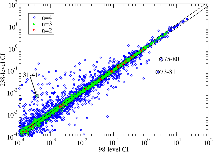
Figure 1: A comparison of $y_{\infty}$ (see eq. 4) for the 98- vs 238-level CI atomic structures for transitions amongst the 98 lowest common levels of Al ⁹⁺. $\circ$: transitions with upper level with $n=2$; $\square$: transitions with upper level with $n=3$; $\diamond$: transitions with upper level with $n=4$; dashed lines: $20\%$ fractional difference.

To illustrate, we show in Fig. 1 a comparison of the reduced quantity $y_{\infty}$, given by

$$y_{\infty}\ =\ \Omega^{\rm PWB}_{\infty}\quad\mbox{ or}\quad\frac{4S}{3}\,,$$ (4)

for the two atomic structure calculations which we consider (which we label 98-level CI and 238-level CI). We show points for a total of 4035 transitions resulting from the common 98 levels. These split into 1466 dipole transitions and 2569 Born-allowed transitions, while there are an additional 718 forbidden transitions that are not represented. We highlight by colour and symbol transitions to upper levels with $n=2,3,4$. We see that transitions up to $n=2$ are very well converged. Only one transition differs by more than $10\%$; it is the very weak ($\sim 10^{-8}$) Born transition $6-9$: $\mathrm{2p^{2}\,{}^{3}P_{0}-2p^{2}\,{}^{1}D_{2}}$ (off the scale). There is good convergence for transitions up to $n=3$, with 233 out of 801 transitions which differ by more than $20\%$ but mostly for the weaker transitions. However, there is much more spread for transitions up to $n=4$, 1834 of 3202 transitions differ by more than $20\%$. This plot illustrates that the $n=4$ levels of the 98-level CI structure are not so well converged with respect to the CI expansion. We expect that their representation by the 238-level CI expansion to be much better converged.

We circle several transitions for comment. The transition $31-41$: $\mathrm{2p3p\,^{3}P_{1}-2p3d\,^{3}P_{2}^{o}}$ is a dipole one, its line strength changes by a factor of 18 between the 98- and 238-level structures. Note also the transitions $75-80$: $\mathrm{2p4d\,^{1}D_{2}^{o}-2p4f\,^{1}F_{3}}$ and $73-81$: $\mathrm{2p4d\,^{3}F_{2}^{o}-2p4f\,^{3}F_{3}}$. Both transitions are dipole allowed and quite strong and yet differ by about a factor of 20 and 30 between the two structures. These levels lie towards the upper end of the 98-level CI expansion. These differences highlight the need for as accurate an atomic description as possible to obtain the best target for accurate collision data and the need to exercise extreme caution when making comparisons of collision data based on different atomic structures.

4 Collisions

In this section, we carry-out a series of comparisons of effective collision strengths for Al ⁹⁺ at the temperature of peak abundance for an electron collisional plasma (Bryans et al. 2006). We then look at issues relating in particular to low temperature (e.g. photoionized) plasmas and much higher temperature plasmas (e.g. solar flares).

4.1 Peak abundance temperature

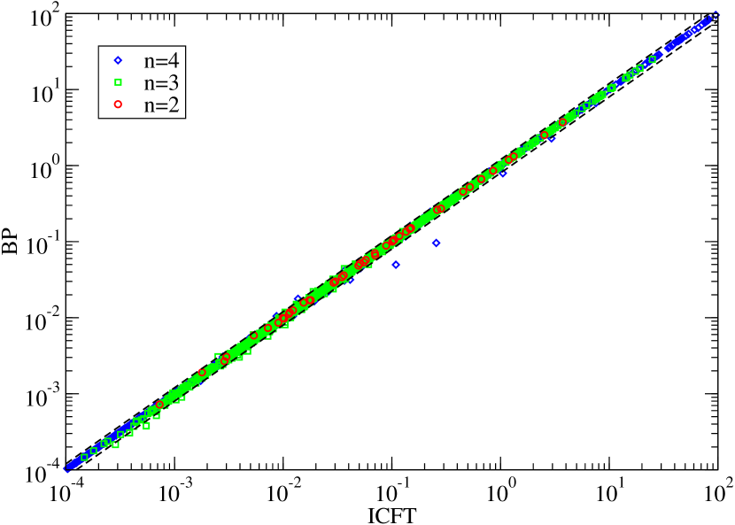
Figure 2: A comparison of effective collision strengths from 98-level CI/CC ICFT versus Breit–Pauli $R$-matrix calculations for all inelastic transitions amongst the 98 levels of Al ⁹⁺ at $T_{\mathrm{e}}=10^{6}\,\mathrm{K}$. $\circ$: transitions with upper level $n=2$; $\square$: transitions with upper level $n=3$; $\diamond$: transitions with upper level $n=4$; dashed lines: $20\%$ fractional difference.

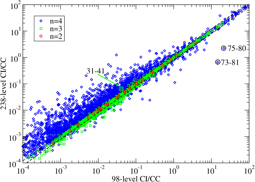
Figure 3: A comparison of effective collision strengths from 98- vs 238-level CI/CC ICFT $R$-matrix calculations for all inelastic transitions amongst the 98 lowest common levels of Al ⁹⁺ at $T_{\mathrm{e}}=10^{6}\,\mathrm{K}$. $\circ$: transitions with upper level $n=2$; $\square$: transitions with upper level $n=3$; $\diamond$: transitions with upper level $n=4$; dashed lines: $20\%$ fractional difference.

In Fig. 2 we compare our 98-level CC ICFT and Breit–Pauli $R$-matrix Maxwellian effective collision strengths, $\Upsilon$, for all inelastic transitions in Al ⁹⁺ at the temperature of peak abundance, $10^{6}\,\mathrm{K}$, in an electron collisional plasma. We recall that both calculations use the exact same (98-level CI) structure. We note excellent agreement between the two scattering methods, as illustrated by the points lying on the diagonal, only 82 points out of 4753 have a difference larger than $10\%$. This is to be contrasted with the spread of points shown in Fig. 1 which results from our two different atomic structures.

Only two points differ from the diagonal more than $50\%$, at around $\Upsilon=10^{-1}$, they correspond to the transitions $67-75$: $\mathrm{2p4p\,^{3}D_{2}-2p4d\,^{1}D_{2}^{o}}$ and $83-98$: $\mathrm{2p4f\,^{3}F_{2}-2p4d\,^{1}P_{1}^{o}}$. Both are dipole allowed through spin–orbit mixing only. It is likely that including the spin–orbit interaction in the collision calculation causes the difference, providing additional mixing via the $(N+1)$-electron Hamiltonian diagonalization.

Next, in Fig. 3 we compare our 98- versus 238-level CI/CC ICFT effective collision strengths as a whole. In contrast to Fig. 2, we see a much wider spread of points, i.e. the agreement between different scattering methods is much (much) better than that obtained using different configuration interaction basis sets. Like the comparison of line strengths and $\Omega^{\rm PWB}_{\infty}$ shown in Fig. 1, we note the excellent and very good agreement between the two sets of results for transitions up to $n=2$ and $n=3$, respectively, while there is a much wider spread in the comparison for transitions up to $n=4$. However, unlike the atomic structure comparison, there is a systematic shift above the diagonal. The 238-level CC results are systematically larger than the 98-level ones. Thus, we conclude that this is not due to the differences in atomic structure, which were evenly distributed above and below the diagonal, rather that this is a measure of the lack of convergence of the close-coupling expansion in the 98-level CC calculation for the transitions involving $n=4$ levels. This mirrors the lack of convergence of the 98-level configuration interaction expansion for $n=4$ levels. We note that there are still more than one hundred levels which lie above the $n=4$ levels in the 238-level CI/CC case.

Specifically, one half of the transitions in Fig. 3 differ by more than $30\%$. The number of transitions differing by more than $20\%$ (lines indicated in the plot) correspond to 1 for $n=2$ (out of 45), 256 for $n=3$ (out of 990) and 2331 for $n=4$ (out of 3718). Note also that the 3 transitions which were circled in Fig. 1 are again circled in Fig. 3. The strong transitions $75-80$ and $73-81$ do illustrate how outliers in the atomic structure comparison (factor 20 and 30 difference) show-up as outliers in the collision comparison (factor 10 and 20 difference). For the weaker transition $31-41$ the resonances in the collision calculation “dampen” the difference in atomic structure, it being “just” a factor of $1.6$ now. In Table 3 we give the exact number of transitions which have a difference $\delta=|\Upsilon_{98}-\Upsilon_{238}|/\Upsilon_{238}$ larger than a given percentage for the $y_{\infty}$ for the 98- vs 238-level CI atomic structures as well as the $\Upsilon$ at $T=10^{6}\,\mathrm{K}$ for the 98-level CC ICFT vs Breit–Pauli and the 98- vs 238-level CC ICFT comparisons.

We can confirm further that the systematic increase of the effective collision strengths to $n=4$ in the 238-level CC calculation over those of the 98-level CC calculation is due to the lack of convergence of the close-coupling expansion in the latter. Like the convergence of the CI expansion, the convergence of the close-coupling expansion is essentially independent of the coupling scheme, i.e. the specific $R$-matrix method used, be it LS, ICFT, Breit–Pauli or DARC. We illustrate this in Fig. 4 where we make a similar comparison of 54- vs 130-term CC $LS$-coupling $R$-matrix effective collision strengths. We see the same systematic increase for transitions to $n=4$ as in the comparison of ICFT $R$-matrix effective collision strengths.

Table 3: Number of transitions in Figs 1 – 3 which differ by more than a certain relative error $\delta=|\Upsilon_{98}-\Upsilon_{238}|/\Upsilon_{238}$ (or $\Upsilon\rightarrow y_{\infty}$), as a percentage.

	Fig. 1: $y_{\infty}$	Fig. 2: 98 CI/CC $\Upsilon$	Fig. 3: ICFT $\Upsilon$
Rel. error ($\%$)	98 vs 238 CI	BP vs ICFT	98 vs 238 CI/CC
1	3778	1336	4579
2	3600	803	4400
3	3416	500	4243
4	3266	350	4077
5	3141	260	3928
6	3022	206	3798
7	2914	158	3676
8	2804	127	3569
9	2722	106	3460
10	2644	82	3357
20	2068	22	2582
30	1643	9	2090
40	1356	4	1725
50	1163	2	1449
75	846	2	1113
100	707	2	901
150	538	1	647
200	443	0	505
300	336	0	320
1000	187	0	88
Total	4035	4753	4753

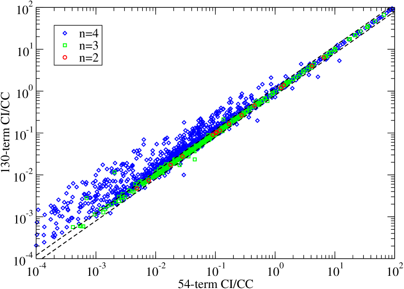
Figure 4: A comparison of effective collision strengths from 54- vs 130-term CI/CC $LS$-coupling $R$-matrix calculations for all inelastic transitions amongst the 54 lowest common terms of Al ⁹⁺ at $T_{\mathrm{e}}=10^{6}\,\mathrm{K}$. $\circ$: transitions with upper term $n=2$; $\square$: transitions with upper term $n=3$; $\diamond$: transitions with upper term $n=4$; dashed lines: $20\%$ fractional difference.

The plots we have shown so far are useful in the respect that they allow us to make comparisons as a function of the strength of a transition — larger differences are acceptable for weaker transitions. On the other hand, because of the wide range of strengths, it is necessary for such plots to be logarithmic. If we plot the ratio of results from two different calculations we can make a linear comparison. We do this in Fig. 5 for the same comparison as we made in Fig. 3, and with respect to the lower level of the transition (5(a)) or the upper one (5(b)). Fig. 5(a) shows that the transitions with the largest scatter are those from $2\mathrm{s}\,3l$ (lower level index 11–20) and $2\mathrm{s}\,4l$ (lower level index 47–60) up to $n=4$, and where we have highlighted by symbol / colour all upper levels with the same $n$-value. It bears a very strong resemblance to the same comparison (figure 2) made by Aggarwal & Keenan (2015a) to compare the 98-level CI/CC DARC effective collision strengths with the 238-level CI/CC ICFT ones, except that they did not differentiate (highlight) the different $n$-values of the upper levels. In contrast, 5(b) clarifies that the differences in the effective collision strengths become increasingly larger as the upper levels excited move closer to the last one included in the 98-level CC calculation. This in turn means that the effective collision strengths to the uppermost levels of the 238-level CC calculation of Fernández-Menchero et al. (2014a) are increasingly unconverged with respect to the close-coupling expansion. However, based on the present convergence study to $n=2$ and $n=3$ we can expect that their results for transitions up to $n=4$ to be well converged, but those to $n=5$ less so since only a partial set of $n=6,7$ levels (to $l=2$) were included in their close-coupling expansion.

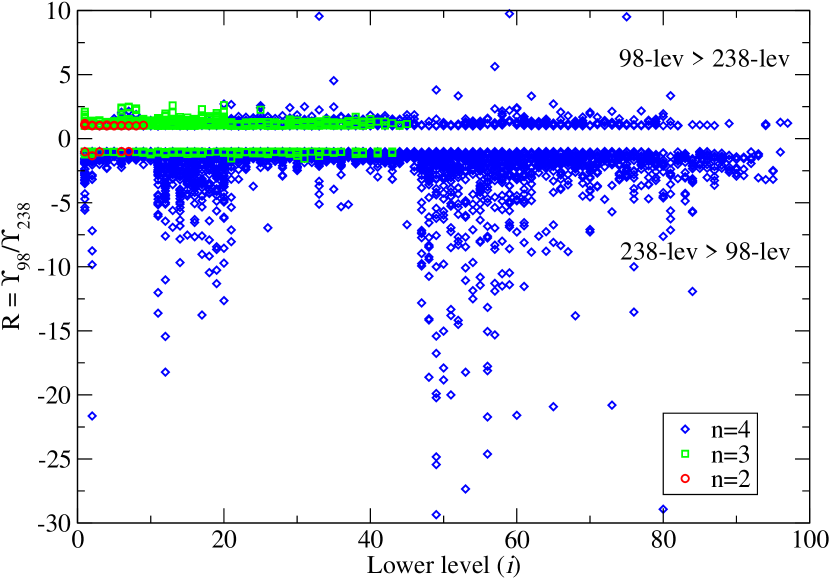
(a)

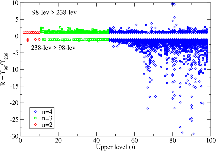
(b)

Figure 5: The ratio of effective collision strengths from 98- vs 238-level CI/CC ICFT $R$-matrix calculations vs (a) lower level and (b) upper level index, for all inelastic transitions amongst the 98 lowest common levels of Al ⁹⁺ at $T_{\mathrm{e}}=10^{6}\,\mathrm{K}$. Positive values indicate $\Upsilon_{98}>\Upsilon_{238}$ and negative values $\Upsilon_{238}>\Upsilon_{98}$. $\circ$: transitions with upper level $n=2$; $\square$: transitions with upper level $n=3$; $\diamond$: transitions with upper level $n=4$.

While all of the plots shown so far are visually appealing, especially Fig. 5, none of them give any indication of the number of transitions whose quantities differ by any given amount — we cannot tell the density of points close to the diagonal (Figs 1–4) or sitting at unity (Fig. 5). We must be wary of such plots misleading us as to the level of agreement, as opposed to disagreement. Only a table like Table 3 gives such an answer.

Thus, these comparisons demonstrate that the observation by Aggarwal & Keenan (2015a), that the 238-level CC effective collisions strengths of Fernández-Menchero et al. (2014a) are systematically and increasingly larger with higher excitations than the 98-level CC results of Aggarwal & Keenan (2014c) over a wide range of temperatures is correct, but it is due to the lack of convergence of the CC expansion of the 98-level CC results of Aggarwal & Keenan (2014c), particularly with respect to the $n=4$ levels.

Finally, there is in fact is good accord between comparable calculations, viz. 98-level CI/CC, we make such a comparison of ICFT vs DARC in Fig. 6. The increasing difference seen as one progresses to higher levels is a reflection of the increasing lack of convergence in the atomic structure. While both use the same CI expansion, there is no reason for both to give the same unconverged result. It is interesting to note that the weakest transitions, mostly forbidden ones, show better agreement than some of the stronger allowed ones. Aggarwal & Keenan (2015a) have already made a detailed comparison of 98-level CI/CC DARC and 238-CI/CC ICFT effective collisions strengths for transitions from the ground state. They highlighted several transitions to $n=4$ which were discrepant, particularly at high temperatures. We consider them in detail in Sec. 4.3

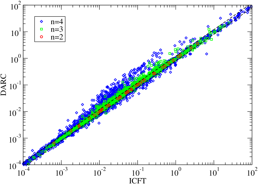
Figure 6: A comparison of effective collision strengths from 98-level CI/CC ICFT versus Dirac $R$-matrix (Aggarwal & Keenan 2014c) calculations for all inelastic transitions amongst the 98 levels of Al ⁹⁺ at $T_{\mathrm{e}}=10^{6}\,\mathrm{K}$. $\circ$: transitions with upper level $n=2$; $\square$: transitions with upper level $n=3$; $\diamond$: transitions with upper level $n=4$; dashed lines: $20\%$ fractional difference.

4.2 Low temperature

The effective collision strengths that we have presented so far have been relevant to the temperature of peak abundance (of Al ⁹⁺) in an electron collisional plasma, such as found in the solar atmosphere and magnetic fusion devices. In photoionized plasmas the same charge state exists at much lower temperatures. The role of resonances becomes more important at low temperatures both with respect to their magnitude, resolution and, in particular, their position. Fernández-Menchero et al. (2014a) carried-out an exhaustive analysis of the convergence of the effective collision strengths with respect to the energy step used to map-out the resonances. They calculated the effective collision strengths $\Upsilon$ by convolution of the ordinary collision strengths $\Omega$ with a Maxwellian electron energy distribution. Then they reduced the energy step by a factor one half and re-calculated $\Upsilon$. After repeatedly reducing the energy step down to a factor one eighth from the original one, the worst case transition from the ground state, the $1-78$, only changed by 10% relative to the previous value of $\Upsilon$, at the lowest temperature calculated of $2\times 10^{4}\,\mathrm{K}$, and by $1\%$ at $10^{6}\,\mathrm{K}$.

We note that Aggarwal & Keenan (2015a) incorrectly reported the energy step used in the resonance region by Fernández-Menchero et al. (2014a). As they stated, Fernández-Menchero et al. (2014a) used an energy step in the resonance region that scales as $\sim z$ in the ion charge, not $z^{2}$, along the sequence. In particular the step length used was $6.94\times 10^{-6}z^{2}\,\mathrm{Ry}$ for Al ⁹⁺, $4.89\times 10^{-6}z^{2}\,\mathrm{Ry}$ for $\mathrm{Cl}^{13+}$, $4.09\times 10^{-6}z^{2}\,\mathrm{Ry}$ for $\mathrm{K}^{15+}$, $3.30\times 10^{-6}z^{2}\,\mathrm{Ry}$ for $\mathrm{Ti}^{18+}$, and $2.02\times 10^{-6}z^{2}\,\mathrm{Ry}$ for $\mathrm{Ge}^{28+}$. These steps are comparable to the ones used by Aggarwal & Keenan (2012, 2014a, 2014c), being slightly finer for Al ⁹⁺, and slightly coarser for $\mathrm{Ge}^{28+}$. Fernández-Menchero et al. (2014a) used this fine mesh only over $2J=1-23$, which corresponds to their exchange calculation. They used their coarse energy mesh across the resonance region as well for $2J=25-89$. Such $J$-values can only give rise to high-$n$ resonances, which by definition are narrow. A simple calculation with autostructure reveals that the strongest resonances have widths $<10^{-5}$ Ryd. Thus, the results provided by Fernández-Menchero et al. (2014a) are converged with respect to the collision energy step and all significant resonances are well resolved. Differences in low temperature effective collision strengths between Aggarwal & Keenan (2014c) and Fernández-Menchero et al. (2014a) can not be ascribed to the resolution of the resonances.

The largest source of error in the low temperature effective collision strengths arises from the inaccuracy in the positioning of resonances which lie just above threshold when the temperature (in energy units) starts to become comparable in magnitude with the uncertainty in position of these resonances. To a first approximation, this uncertainty in position is given by the difference between the calculated and observed values for the energy level to which the resonance is attached. In general, the specific level is not know, without detailed resonance analysis. Energy level accuracy can be improved theoretically via the use of pseudostates or purely ‘experimentally’ through the use of observed energies or by a combination of theory and observation using term energy corrections. Each has its limitations: the use of pseudostates can lead to pseudoresonances at higher energies while not all levels may be known observationally. Storey et al. (2014) discuss the various considerations that need to be made in order to calculate accurate data at very low temperatures for planetary nebulae, for example.

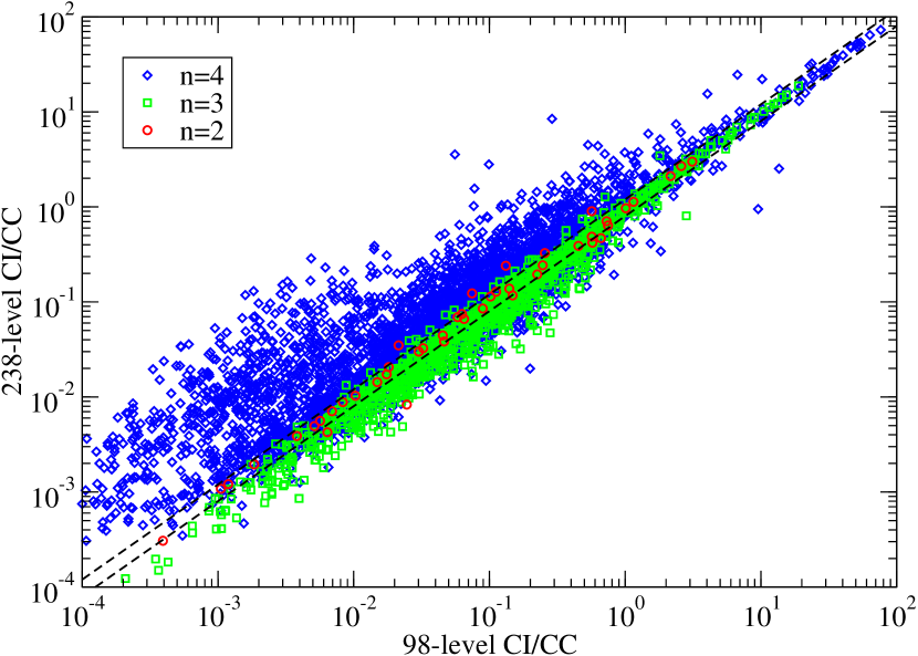
Figure 7: A comparison of effective collision strengths from 98- vs 238-level CI/CC ICFT $R$-matrix calculations for all inelastic transitions amongst the 98 lowest common levels of Al ⁹⁺ at $T_{\mathrm{e}}=2\times 10^{4}\,\mathrm{K}$. $\circ$: transitions with upper level $n=2$; $\square$: transitions with upper level $n=3$; $\diamond$: transitions with upper level $n=4$; dashed lines: $20\%$ fractional difference.

Fig. 7 shows a comparison of 98- and 238-level CC ICFT effective collision strengths for transitions between the lowest common 98 levels of Al ⁹⁺ at a photoionized plasma temperature of $2\times 10^{4}\,\mathrm{K}$ (Kallman & Bautista 2001). The same energy grid was used in both cases in the resonance region. Differences are much larger than the ones seen at the temperature of peak abundance in an electron collisional plasma, even for transitions between the low-lying levels ($n=2$). The increased differences in the effective collision strengths is likely due to the position of the resonances, especially where the 238-level CC effective collision strengths are smaller than the 98-level ones. In addition, the systematic enhancement of the effective collision strengths to $n=4$ levels due to resonances attached to $n>4$ is increased due to the greater relative contribution from resonances; i.e. the lack of convergence of the close-coupling expansion for these levels in the 98-level calculation becomes even more significant. However, at low temperatures, most modelling applications involve transitions from the ground state, and perhaps a metastable. The factor $\exp(-\Delta E/kT)$ arising in the excitation rate coefficient means that only the lowest few excited levels are of interest, i.e. transitions within $n=2$.

The inaccuracy in the position of the resonances makes effective collision strengths from both Fernández-Menchero et al. (2014a) and Aggarwal & Keenan (2012, 2014a, 2014c) increasingly unreliable at low temperatures. For example, if we shift all resonances down in energy by $0.002$ Ryd (comparable with the accuracy of some energy levels) then the effective collision strength for the $1-4:\mathrm{2s^{2}\,{}^{1}S_{0}-2s2p\,^{3}P_{2}^{o}}$ transition changes by a factor of 2 at $2\times 10^{4}\,\mathrm{K}$, although this is reduced to a $20\%$ effect by $2\times 10^{5}\,\mathrm{K}$. Nevertheless, such results can be used for estimation purposes.

4.3 High temperature

We calculate effective collision strengths over a wide range of temperatures, as defined by the OPEN-ADAS adf04 file format viz. $2\times 10^{2}-2\times 10^{6}\;(z+1)^{2}$ K, to cover all possible applications to electron-collisional plasmas. Higher temperature effective collision strengths require ordinary collision strengths to higher energies, which in turn require the contribution from higher partial waves, and this needs to be handled efficiently and accurately by $R$-matrix calculations.

Aggarwal & Keenan (2015a) highlighted several transitions ($1-64$, $1-70$ and $1-80$) for which they observed large differences between the 238-level CI/CC ICFT results of Fernández-Menchero et al. (2014a) and the 98-level CI/CC DARC ones of Aggarwal & Keenan (2014c), particularly at high temperatures. They suggested that the use of the Burgess & Tully (1992) formulae at high energy was perhaps a major source of error, i.e. that the ICFT calculations did not go high enough in energy for the collision strengths to have reached their asymptotic form. Aggarwal & Keenan (2015a) also commented-on the neglect of electron exchange by Fernández-Menchero et al. (2014a) at high-$J$.

The ‘top-up’ procedure used for angular momentum is described in Fernández-Menchero et al. (2014a). In addition, Fernández-Menchero et al. (2014a) included electron exchange for angular momenta up to $2J=23$, and then used a non-exchange calculation for the rest of the angular momenta calculated: $2J=25-89$. (Aggarwal & Keenan (2014c) included exchange for all of the angular momenta calculated, up to $2J=91$.) The method used by Fernández-Menchero et al. (2014a) is not a source of significant inaccuracy. By $2J=25$ the smallest exchange multipole is larger than $10$. Neglect of higher exchange multipoles causes a small underestimate at the highest temperatures for a few very weak highly forbidden transitions, i.e. ones that not only have no target mixing with allowed transitions (i.e. zero limit points) but also are not strongly enhanced by coupling. By extending the inclusion of exchange to $2J=51$ we find no transition differing by more than $5\%$ up to $2\times 10^{7}\,\mathrm{K}$, rising to $10\%$ at $2\times 10^{8}\,\mathrm{K}$, for Al ⁹⁺.

With regards to energy, Fernández-Menchero et al. (2014a) extended the outer region $R$-matrix calculation up to three times the ionization potential, $88\,\mathrm{Ry}$ in the case of Al ⁹⁺. They then carried-out a linear interpolation of the reduced collision strength, $y$, as a function of the reduced scattering energy, $x\in[0,1]$, for dipole and Born allowed transitions (while forbidden transitions were extrapolated) as follows.

For a given excitation, let $E$ denote the final scattered energy (with $\Delta E$ the excitation energy still) and define

$$\varepsilon\ =\ \frac{E}{\Delta E}\,.$$ (5)

Then, at threshold ($E=0$) $\varepsilon=0$. Following Burgess & Tully (1992), we divide all transitions into one of three cases to represent $(x,y)$, based-on their infinite energy values $y_{\infty}$, or lack thereof, as described in sec. 3.

• Dipole transitions

  $$x = 1\ -\ \frac{\ln C}{\ln\left(\varepsilon\,+\,C\right)}$$

  $$y = \frac{\Omega}{\ln\left(\varepsilon\,+\,\mathrm{e}\right)}$$ (6)

• Born transitions

  $$x = \frac{\varepsilon}{\varepsilon\,+\,C}$$

  $$y = \Omega$$ (7)

• Forbidden transitions

  $$x = \frac{\varepsilon}{\varepsilon\,+\,C}$$

  $$y = \left(\varepsilon\,+\,1\right)^{\alpha}\,\Omega$$ (8)

where $C$ is an arbitrary visual scaling parameter. In the last case, formally, $\alpha=2$ in the infinite energy limit. At high but finite energies, a more accurate approach is to determine $\alpha$ from two reasonably well-separated high-energy points so as to take account of enhancement or depletion of these weak high-energy collision strengths by continuum coupling. This is carried-out automatically, but restricted to the range $\alpha=1-3$, i.e. within reasonable physical bounds.

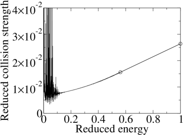
(a) $1-52:\mathrm{2s^{2}\,{}^{1}S_{0}-2s4p\,^{1}P_{1}^{o}}$

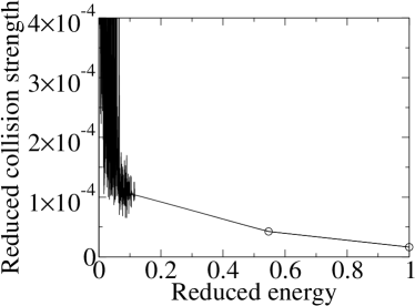
(b) $1-64:\mathrm{2s^{2}\,{}^{1}S_{0}-2p4s\,^{1}P_{1}^{o}}$;

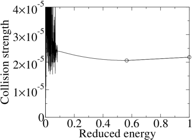
(c) $1-70:\mathrm{2s^{2}\,{}^{1}S_{0}-2p4p\,^{3}P_{0}}$

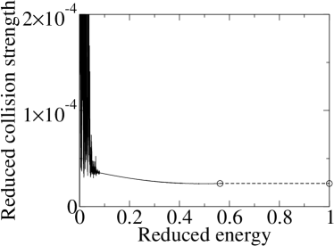
(d) $1-80:\mathrm{2s^{2}\,{}^{1}S_{0}-2p4f\,^{1}F_{3}}$

Figure 8: Reduced collision strengths versus energy from 238-level CI/CC ICFT $R$-matrix calculations for selected transitions of Al ⁹⁺. $\circ$: denotes the last finite calculated and infinite energy points; dashed line: indicates extrapolation for a forbidden transition. ($C=2.$)

Fig. 8 shows the reduced collision strength in a Burgess–Tully $(x,y)$ plot from the 238-level CI/CC ICFT calculation for Al ⁹⁺ by Fernández-Menchero et al. (2014a). Fig. 8(a) is for a strong dipole transition $1-52:\mathrm{2s^{2}\,{}^{1}S_{0}-2s4p\,^{1}P_{1}^{o}}$, Fig. 8(b) the dipole transition $1-64:\mathrm{2s^{2}\,{}^{1}S_{0}-2p4s\,^{1}P_{1}^{o}}$ which takes place through configuration mixing, Fig. 8(c) the Born-allowed transition $1-70:\mathrm{2s^{2}\,{}^{1}S_{0}-2p4p\,^{3}P_{0}}$ which also takes place only through configuration mixing, and Fig. 8(d) is for the forbidden transition $1-80:\mathrm{2s^{2}\,{}^{1}S_{0}-2p4f\,^{1}F_{3}}$ which is a very weak two-electron jump. An automatically determined value of $\alpha=1$ for this transition was used to extrapolate the reduced collision strength as a function of reduced energy — see equation 8. Fig. 8 shows that all of the transitions have reached the assumed asymptotic form. What then is the source of the differences in high temperature effective collision strengths noted by Aggarwal & Keenan (2015a)? The answer lies in the atomic structure.

In Table 4 we compare effective collision strengths from the 98- and 238-level CI/CC ICFT calculations with the 98-level CI/CC DARC ones (Aggarwal & Keenan 2014c). We note first that results for the strong dipole transition $1-21$ are independent of atomic structure (98- vs 238-level CI $y_{\infty}=4S/3$) and close-coupling expansion (98- vs 238-level CC $\Upsilon$). However, if we consider the weak dipole transition $1-64$ we see that the limit value ($y_{\infty}$) is a factor 6.2 larger for the 98- vs 238-level CI (Breit–Pauli) case and this leads to a factor of 2.08 in the corresponding ICFT effective collision strengths at $2\times 10^{7}\,\mathrm{K}$. Indeed, the difference in effective collision strengths would likely be larger were it not for the fact that the 238-level CI/CC is (much) larger at (much) lower temperatures due to additional resonances and coupling. The DARC structure limit point reported by Aggarwal & Keenan (2015a) is similar to the 98-level CI Breit–Pauli one. Correspondingly, the 98-level CI/CC DARC and ICFT effective collision strengths agree to within $\sim 20\%$ over the entire temperature range shown in Table 4.

For the case of the (weak) Born-allowed transition $1-70$ we see a similar trend in the comparisons, viz. differences in structure ($y_{\infty}$) leading to corresponding differences in high temperature effective collision strengths, strong resonance enhancement at lower temperature for the 238- vs 98-level CI/CC results and agreement to within 30% between the DARC and ICFT 98-level CI/CC results. (Aggarwal & Keenan (2015a) do not report Born limits for this transition, but clearly the sensitivity to atomic structure we see reflected in the two Breit–Pauli Born limits accounts for the remaining difference.) Finally, for the weak forbidden $1-80$ transition we note a very similar set of comparisons as for the $1-70$ transition, indeed, the DARC and ICFT 98-level CI/CC results agree more closely (20%). The 238-level CI/CC ICFT result is increasingly enhanced by resonances over the 98-level CI/CC one at low temperatures, by a factor 15 at $2\times 10^{4}$ K. We note that including higher-$J$ exchange multipoles does not change the effective collision strength to 3 s.f. even at the highest temperature considered. There are several equally forbidden transitions ($1-61,68,69$, not shown) for which the pattern of dis/agreement is very similar to that for the $1-80$, in all cases.

In summary, the results of the 98-level CI/CC DARC calculation of Aggarwal & Keenan (2014c) are in much closer agreement (indeed, no significant differences) with the present 98-level CI/CC ICFT results than the 238-level CI/CC ones across a wide range of temperatures for all of the transitions highlighted by Aggarwal & Keenan (2015a). However, the results of the calculations obtained using the 238-level CI target have a better converged atomic structure and, correspondingly, give more accurate effective collision strengths, especially at high temperatures, while the much better convergence of the 238-level close-coupling expansion provides more accurate results across a wide range of temperatures.

Table 4: Comparison of effective collision strengths, $\Upsilon$, at selected finite temperatures, and the reduced quantity $y_{\infty}$ at infinite temperature. See Table 2 for the transition indices $i,j$.

		DARC				ICFT
$i$–	$j$	98-level CI/CC				98-level CI/CC					238-level CI/CC
$T$(K)		$2\times 10^{4}$	$10^{6}$	$2\times 10^{7}$		$2\times 10^{4}$	$10^{6}$	$2\times 10^{7}$	$\infty$		$2\times 10^{4}$	$10^{6}$	$2\times 10^{7}$	$\infty$
1–	52	$1.09\,(-2)$	$1.01\,(-2)$	$3.01\,(-2)$		$1.14\,(-2)$	$1.02\,(-2)$	$3.20\,(-2)$	$2.40\,(-2)$		$1.53\,(-2)$	$9.68\,(-3)$	$3.22\,(-2)$	$2.64\,(-2)$
1–	64	$5.49\,(-4)$	$1.78\,(-4)$	$1.70\,(-4)$		$5.80\,(-4)$	$1.80\,(-4)$	$1.96\,(-4)$	$1.01\,(-4)$		$3.12\,(-3)$	$2.94\,(-4)$	$9.40\,(-5)$	$1.63\,(-5)$
1–	70	$2.68\,(-5)$	$1.26\,(-5)$	$5.29\,(-6)$		$3.48\,(-5)$	$1.11\,(-5)$	$4.24\,(-6)$	$2.68\,(-6)$		$6.99\,(-5)$	$3.10\,(-5)$	$2.18\,(-5)$	$2.18\,(-5)$
1–	80	$4.52\,(-5)$	$2.51\,(-5)$	$8.45\,(-6)$		$4.63\,(-5)$	$2.47\,(-5)$	$7.05\,(-6)$	$-$		$7.04\,(-4)$	$8.66\,(-5)$	$1.09\,(-5)$	$-$

Notes. DARC: Aggarwal & Keenan (2014c); 98-level ICFT: present work; 238-level ICFT: Fernández-Menchero et al. (2014a). $A\,(B)$ denotes $A\times 10^{B}$.

5 Conclusions

Reliable and accurate electron-impact excitation data are key to the successful spectroscopic diagnostic modelling of non-LTE plasmas. We have compared and contrasted differences in such data for the benchmark Be-like Al ⁹⁺ ion which we have calculated using the $R$-matrix method. Such differences arise through: 1) differing approximations of relativistic effects, 2) uncertainties in atomic structure and 3) errors due to the lack of convergence of the close-coupling expansion. Error 3) is quantifiable and can be reduced systematically and reliably — we illustrated this by comparing new 98-level and previous 238-level CC ICFT $R$-matrix calculations. We find that effective collision strengths to $n=4$ levels are significantly enhanced over a wide range of temperatures by coupling to $n>4$ levels. Uncertainty 2) is quantifiable but is more difficult to reduce and constrain as an error — we compared 98-level and 238-level configuration interaction expansion calculations of line strengths and infinite energy plane-wave Born collision strengths to illustrate this point. Again, transitions to $n=4$ levels are most susceptible to lack of convergence but now of the configuration interaction expansion. Differences 1) between ICFT and Breit-Pauli $R$-matrix treatments of relativistic effects are small, and negligible relative to 2) and 3), as is to be expected for an element which lies below Zn. We illustrated this by a comparison of new 98-level CI/CC ICFT and Breit–Pauli $R$-matrix effective collision strengths which use the exact same atomic structure. We also find good accord between our 98-level CI/CC results and previous ones from a 98-level CI/CC Dirac–Coulomb $R$-matrix calculation, particularly for transitions from the ground-level.

However, based-upon the study of effects 1), 2) and 3), we conclude that the original 238-level CI/CC ICFT $R$-matrix results are the most complete to-date with respect to convergence of both the configuration interaction and close-coupling expansions and a reliable treatment of relativistic effects. Or to put it more simply, the earlier 238-level CI/CC ICFT work (Fernández-Menchero et al. 2014a) has a superior target to the 98-level CI/CC DARC one (Aggarwal & Keenan 2014c) and provides more accurate atomic data.

Thus, we find to be false the recent conjecture by Aggarwal & Keenan (2015a) that the ICFT approach may not be completely robust. Their conjecture was based upon a comparison of 98-level CI/CC Dirac $R$-matrix effective collision strengths (Aggarwal & Keenan 2014c) with those from 238-level CI/CC ICFT $R$-matrix calculations (Fernández-Menchero et al. 2014a). Rather, Aggarwal & Keenan (2015a) have failed to appreciate the size of the effect which the lack of convergence, in both the close-coupling and configuration interaction expansions, has on transitions to the higher-lying states ($n=4$ in the case of a 98-level CI/CC expansion for Al ⁹⁺). This can only be quantified by extending the expansions.

There is nothing special about Al ⁹⁺ with regards to the convergence of the close-coupling expansion. Except perhaps at the lowest charge states, as they discussed, the effective collision strengths for all ions in the $\mathrm{Be}$-like sequence, from $\mathrm{B}^{+}$ to $\mathrm{Kr}^{32+}$ calculated by Fernández-Menchero et al. (2014a) using the 238 level CI/CC expansion are the most complete and reliable to-date. The use of a 98 level CI/CC expansion for Al ⁹⁺ (Aggarwal & Keenan 2014c), $\mathrm{Cl}^{13+}$, $\mathrm{K}^{15+}$, $\mathrm{Ge}^{28+}$ (Aggarwal & Keenan 2014a) and $\mathrm{Ti}^{18+}$ (Aggarwal & Keenan 2012) means that these effective collision strengths for transitions up to $n=4$ are increasingly an underestimate over a wide range of temperatures, including the temperature of peak abundance.

There is nothing special about $\mathrm{Be}$-like ions. The 136-level CC DARC calculations of Aggarwal & Keenan (2014b) for $\mathrm{Fe}^{13+}$ are shown to be a systematic underestimate compared to the 197-level CC ICFT calculations of Liang et al. (2010) (in addition, Liang et al. used a much larger CI expansion 2985 vs 136 levels) — see Del Zanna et al (MNRAS to be submitted) for another detailed analysis similar to the present paper’s. The convergence of the close-coupling expansion increasingly affects the accuracy of collision data to the highest-lying states in all $R$-matrix calculations. Likewise, the accuracy of the atomic structure becomes more uncertain for the most highly-excited states of the configuration interaction expansion.

In general, care must be exercised when comparing collision data calculated using different atomic structures and / or close-coupling expansions lest one draws false conclusions. Finally, given Figs 1 and 3 and Table 3, we suggest that it is fanciful to assign a single accuracy rating of $20\%$, say, to an entire collision data set.

Appendix A C²⁺

Just recently, another paper by Aggarwal & Keenan (2015b) has appeared, this time on Be-like $\mathrm{C}^{2+}$, making much the same claims that have just been refuted, quite generally, above. Aggarwal & Keenan (2015b) have extended their CI/CC expansion up to $n=5$ this time, but this 166-level expansion still falls short of the 238-level expansion up to $nl=7\mathrm{d}$ of Fernández-Menchero et al. (2014a). This may reduce the systematic differences (understimates) of their results up to $n=4$ somewhat compared to those of Fernández-Menchero et al. (2014a) but the low-charge state means that the errors and uncertainties due to the difference between the two atomic structures will be much larger than for $\mathrm{Al}^{9+}$. Arguably, a Breit–Pauli $R$-matrix with pseudo-states calculation is required for $\mathrm{C}^{2+}$ to give a definitive representation of the CI/CC expansion for all level-resolved transitions.

References

- Aggarwal & Keenan (2012) Aggarwal K. M., Keenan F. P., 2012, Phys. Scr., 86, 055301
- Aggarwal & Keenan (2014a) Aggarwal K. M., Keenan F. P., 2014a, Phys. Scr., 89, 125401
- Aggarwal & Keenan (2014b) Aggarwal K. M., Keenan F. P., 2014b, Mon. Not. R. Astr. Soc., 445, 2015
- Aggarwal & Keenan (2014c) Aggarwal K. M., Keenan F. P., 2014c, Mon. Not. R. Astr. Soc., 438, 1223
- Aggarwal & Keenan (2015a) Aggarwal K. M., Keenan F. P., 2015a, Mon. Not. R. Astr. Soc., 447, 3849
- Aggarwal & Keenan (2015b) Aggarwal K. M., Keenan F. P., 2015b, Mon. Not. R. Astr. Soc., 0, submitted http://arxiv.org/abs/1503.07673
- Badnell (1999) Badnell N. R., 1999, Journal of Physics B: Atomic, Molecular and Optical Physics, 32, 5583
- Badnell (2011) Badnell N. R., 2011, Comput. Phys. Commun., 182, 1528
- Badnell & Ballance (2014) Badnell N. R., Ballance C. P., 2014, The Astrophysical Journal, 785, 99
- Badnell & Griffin (1999) Badnell N. R., Griffin D. C., 1999, J. Phys. B, 32, 2267
- Berrington et al. (2005) Berrington K. A., Ballance C. P., Griffin D. C., Badnell N. R., 2005, Journal of Physics B: Atomic, Molecular and Optical Physics, 38, 1667
- Berrington et al. (1987) Berrington K. A., Burke P. G., Butler K., Seaton M. J., Storey P. J., Taylor K. T., Yan Y., 1987, Journal of Physics B: Atomic and Molecular Physics, 20, 6379
- Berrington et al. (1995) Berrington K. A., Eissner W. B., Norrington P. H., 1995, Comput. Phys. Commun., 92, 290
- Bryans et al. (2006) Bryans P., Badnell N. R., Gorczyca T. W., Laming J. M., Mitthumsiri W., Savin D. W., 2006, Astrophys. J. Suppl. Ser., 167, 343
- Burgess & Tully (1992) Burgess A., Tully J. A., 1992, Astron. Astrophys., 254, 436
- Fernández-Menchero et al. (2014a) Fernández-Menchero L., Del Zanna G., Badnell N. R., 2014a, Astron. Astrophys., 566, A104
- Fernández-Menchero et al. (2014b) Fernández-Menchero L., Del Zanna G., Badnell N. R., 2014b, Astron. Astrophys., 572, A115
- Griffin et al. (1998) Griffin D. C., Badnell N. R., Pindzola M. S., 1998, J. Phys. B, 31, 3713
- Griffin et al. (1999) Griffin D. C., Badnell N. R., Pindzola M. S., Shaw J. A., 1999, J. Phys. B, 32, 2139
- Hummer et al. (1993) Hummer D. G., Berrington K. A., Eissner W., Pradhan A. K., Saraph H. E., Tully J. A., 1993, Astron. Astrophys., 279, 298
- Kallman & Bautista (2001) Kallman T., Bautista M., 2001, The Astrophysical Journal Supplement Series, 133, 221
- Keenan (1988) Keenan F. P., 1988, Physica Scripta, 37, 57
- Liang & Badnell (2010) Liang G. Y., Badnell N. R., 2010, Astron. Astrophys., 518, A64
- Liang et al. (2010) Liang G. Y., Badnell N. R., López-Urrutia J. R. C., Baumann T. M., Del Zanna G., Storey P. J., Tawara H., Ullrich J., 2010, The Astrophysical Journal Supplement Series, 190, 322
- Liang et al. (2012) Liang G. Y., Badnell N. R., Zhao G., 2012, Astron. Astrophys., 547, A87
- Liang et al. (2009) Liang G. Y., Whiteford A. D., Badnell N. R., 2009, Astron. Astrophys., 500, 1263
- Martin & Zalubas (1979) Martin W. C., Zalubas R., 1979, J. Phys. Chem. Ref. Data, 8, 817
- Storey et al. (2014) Storey P. J., Sochi T., Badnell N. R., 2014, Monthly Notices of the Royal Astronomical Society, 441, 3028