The affine inflation market models

Stefan Waldenberger

Keywords:

Arbitrage-free inflation models have first been rigorously introduced in Jarrow and Yildirim [10]. Since then several inflation models have been proposed. Similar to interest rate models one can distinguish between short rate models and market models. While short rate models in the spirit of Jarrow and Yildirim [10] aim at modeling the unobservable continuous nominal and real short rate, market models use discrete observable rates as the basis for modeling (see Belgrade et al. [1], Mercurio [16]). These observable rates are the basis of liquidly traded inflation swaps, zero coupon inflation-indexed swaps and year-on-year inflation-indexed swaps. While there have been several extensions of these models (e.g. Mercurio and Moreni [17, 18]) all of these models suffer the problem that there exist analytical formulas for only one type of swap, but not both. The model in this paper leads to closed formulas for both types.

Based on the ideas in Keller-Ressel et al. [14] one can use affine processes to describe analytically highly tractable models. Affine processes are Markov process, where the characteristic function is of exponentially affine form, i.e.

$$\mathbb{E}^{\!}\left[\mathrm{e}^{uX_{t}}|X_{s}\right]=\mathrm{e}^{\phi(t-s,u)+\psi(t-s,u)X_{s}}.$$

The class of affine processes contains a large number of processes, e.g. every Lèvy process is affine. Using the longest-dated nominal zero coupon bond as a numeraire we can model the normalized bond prices as “exponential martingales” with respect to an affine process $X$. In this type of models we are not only able to price both types of inflation swaps, but can also derive semianalytical formulas for calls and puts on the underlying inflation rates, another liquidly traded inflation derivative.

The structure of this paper is as follows. The first part describes inflation markets and typical traded derivatives. Afterwards we outline the setup of an inflation market model. The second part introduces the affine inflation market model and derives pricing formulas for the introduced inflation derivatives. The third part provides a concrete model specification including the calibration to actual market data. In the appendix we collect the properties of affine processes needed in this paper. Furthermore we specify the affine processes used in the numerical section.

1 Inflation markets

Denote the time $t$ price of the nominal zero coupon bond with maturity $T$ by $P(t,T)$ and consider an inflation index with time $t$ value $I(t)$. Typically inflation indexes are so-called consumer price indexes (CPI). To shorten notation we will use the term CPI synonymous for inflation index, nevertheless the reader can think of an arbitrary inflation index. The basic mathematical instruments in inflation-linked markets are so called inflation-linked zero coupon bonds (corresponding to zero coupon bonds for nominal interest rate markets). An inflation-linked zero coupon bond with maturity $T$ is a bond paying $I(T)$ at time $T$. Denote its price by $P_{ILB}(t,T)$.

In actual markets governments issue inflation-linked coupon bonds. Such a bond pays a fixed coupon on the variable basis $I(T_{k})/I(T_{0})$ at some fixed number of predetermined dates $T_{k}\leq T$ (typically annually), where $T_{0}$ is the time of issue. Additionally to the coupons such a bond redeems at maturity $T$ with value $\max\{I(T)/I(T_{0}),1\}$. Such a bond can therefore be described as a combination of inflation-linked zero coupon bonds plus an included option with payoff $(1-I(T)/I(T_{0}))_{+}$. In general these bonds are issued with maturities of several years and inflation is positive. In this case the included option has little influence on the total price, which is why it is market practice to mostly ignore it. In particular if one ignores these options it is possible to strip inflation-linked zero coupon bond prices out of actually traded inflation-linked coupon bonds by the same methods used for nominal quantities.

Consider the quantity

$$P_{R}(t,T):=\frac{P_{ILB}(t,T)}{I(t)},$$ (1)

which is called the price of a real zero-coupon bond. Note that this is not the price of a traded asset, but a theoretical quantity. The usage of the term price is motivated by the fact that this quantity can be viewed as the price of a zero coupon bond in a fictitious economy, where everything is measured in terms of the inflation index $I(t)$. Given real zero-coupon bond prices continuously compounded real interest rates are defined by $R(t,T):=-{\,\ln\left(P_{R}(t,T)\right)}/{(T-t)}.$ Accordingly one can define real counterparts to other nominal quantities such as forward interest rates or the short rate. This quantities are sometimes used as a starting point for inflation option pricing models (see e.g. Jarrow and Yildirim [10], Mercurio [16]).

Next to inflation-linked bond markets there exist several liquidly traded inflation-linked derivatives. First consider the forward price of the inflation index (forward CPI), i.e. the at time $t$ fixed value $\operatorname{\mathcal{I}}(t,T)$, which at time $T$ can be exchanged against $I(T)$ without additional costs. Since $P_{ILB}(t,T)$ is the current price of $I(T)$, the time $t$ forward CPI for maturity $T$ is

$$\operatorname{\mathcal{I}}(t,T):=\frac{P_{ILB}(t,T)}{P(t,T)}.$$ (2)

In a zero coupon inflation-indexed swap (ZCIIS) two parties exchange the realized inflation $\frac{I(T)}{I(t)}$ against a fixed amount $(1+K)^{T-t}$. ZCIIS are mostly traded for full year maturities M. For $T=t+M$ the value of such a payer swap can be expressed as

$$P(t,T)\left(\frac{\operatorname{\mathcal{I}}(t,T)}{I(t)}-(1+K)^{M}\right).$$ (3)

The rate $K$, for which equation (3) is zero is then called the ZCIIS rate $ZCIIS(t;M)$. These ZCIIS rates are quoted in the market for several full-year maturities.

Remark.

Note that ZCIIS rates and inflation-linked bonds are closely related via (2) and (3). In reality this relationship is not observed. This is partly due to different creditworthiness of counterparties in bond and swap markets. A more detailed analysis of this difference can be found in Fleckenstein et al. [7]. For model calibration one has to choose one market, usually the swap market.

Next to ZCIIS there is a second important type of swap in inflation markets, the year-on-year inflation-indexed swaps (YYIIS). These swaps exchange the annualized inflation against a fixed rate $K$, i.e. consider an annually spaced tenor structure $T_{k}=t+k,k=0,\dots,M$. The netted payment of a payer YYIIS at time $T_{k}$ is $\left({I(T_{k})}/{I(T_{k-1})}-1\right)-K.$ Hence the inflation leg consists of payoffs of the form

$$\frac{1}{T-S}\left(\frac{I(T)}{I(S)}-1\right).$$

Denote the forward value of such a payoff, the annualized forward inflation rate, by $F_{I}(t,S,T)$. Then the value of a payer YYIIS with maturity $M$ and strike $K$ can be expressed as

$$\sum_{k=1}^{M}P(t,T_{k})(F_{I}(t,T_{k-1},T_{k})-K).$$

The YYIIS rate $YYIIS(t;M)$ is the rate $K$ such that the corresponding YYIIS has zero value. Note that given YYIIS rates for all annual maturities one can calculate annual forward inflation rates $F_{I}(t,T_{k-1},T_{k})$ and vice versa.

Foward CPIs $\operatorname{\mathcal{I}}(t,T)$, respectively forward inflation rates $F_{I}(t,S,T)$ are the mathematical quantities underlying the market-traded ZCIIS, respectively YYIIS. Inflation market models aim at modeling these quantities. In existing inflation market models either $\operatorname{\mathcal{I}}(t,T)$ or $F_{I}(t,S,T)$ can be expressed by analytical formulas, but not both. Consider a market, where price processes are assumed to be semimartingales on a filtered probability space $(\Omega,\mathcal{A},(\mathcal{F}_{t}),\operatorname{\mathbb{P}})$. Fix a $T$-forward measure $\operatorname{\mathbb{Q}}^{T}$, i.e. a probability measure equivalent to $\operatorname{\mathbb{P}}$ such that asset prices normalized with the numeraire price $P(t,T)$ are $\operatorname{\mathbb{Q}}^{T}$-martingales. Then

$$\operatorname{\mathcal{I}}(t,T) =\mathbb{E}^{\operatorname{\mathbb{Q}}^{T}}\left[I(T)|\operatorname{\mathcal{F}}_{t}\right]$$

$$F_{I}(t,S,T) =\operatorname{\mathbb{E}}^{\operatorname{\mathbb{Q}}^{T}}\left[\frac{1}{T-S}\left(\frac{I(T)}{I(S)}-1\right)\bigg{|}\operatorname{\mathcal{F}}_{t}\right].$$

Calculating the expectations of the inflation index, as well as the fraction of the inflation index at two different times proves difficult. In the model of this paper both are exponentially affine in the underlying driving stochastic process. For an affine process (see appendix) such expectations can be calculated and we are able to give semianalytical formulas for many standard options like caps and floors of forward inflation rates.

1.1 The inflation market model

We now introduce the general setup of an (inflation) market model. Consider a tenor structure $0<T_{1}<\dots<T_{N}=:T$ and a market consisting of zero coupon bonds with maturities $T_{k}$ and prices $P(t,T_{k})$. The price processes $(P(t,T_{k}))_{0\leq t\leq T_{k}}$ are assumed to be positive semimartingales on a filtered probability space $(\Omega,\mathcal{A},(\mathcal{F}_{t})_{0\leq t\leq T},\operatorname{\mathbb{P}})$, which satisfy $P(T_{k},T_{k})=1$ almost surely. If there exists an equivalent probability measure $\operatorname{\mathbb{Q}}^{T}$ such that the normalized bond price processes $P(\cdot,T_{k})/P(\cdot,T)$ are martingales, the market is arbitrage-free. This setup describes the class of interest rate market models like the classical LIBOR market model (Brace et al. [2]) and its extensions.

To extend this setup to inflation markets consider an inflation index $I$, where we assume w.l.o.g. that $I(0)=1$. Assume there exist inflation-linked zero-coupon bonds with the same maturities $T_{1},\dots,T_{N}$ and price processes $P_{ILB}(t,T_{k})_{0\leq t\leq T_{k}}$, all of which are positive semimartingales. If there exists an equivalent probability measure $\operatorname{\mathbb{Q}}^{T}$ such that all normalized price processes

$$\left(\frac{P(t,T_{k})}{P(t,T)}\right)_{0\leq t\leq T_{k}},\qquad\left(\frac{P_{ILB}(t,T_{k})}{P(t,T)}\right)_{0\leq t\leq T_{k}}$$ (4)

are $\operatorname{\mathbb{Q}}^{T}$-martingales, the extended market model is arbitrage-free. For given $\operatorname{\mathbb{Q}}^{T}$ define the $T_{k}$-forward measures $\operatorname{\mathbb{Q}}^{T_{k}}$ by

$$\frac{\,\mathrm{d}\operatorname{\mathbb{Q}}^{T_{k}}}{\,\mathrm{d}\operatorname{\mathbb{Q}}^{T}}=\frac{1}{P(T_{k},T)}\frac{P(0,T)}{P(0,T_{k})}.$$ (5)

Under $\operatorname{\mathbb{Q}}^{T_{k}}$ the forward interest rate

$$F^{k}(t):=\frac{1}{\Delta_{k}}\left(\frac{P(t,T_{k-1})}{P(t,T_{k})}-1\right),\qquad\Delta_{k}:=T_{k}-T_{k-1},$$

the earlier introduced forward CPI

$$\operatorname{\mathcal{I}}(t,T_{k})=\frac{P_{ILB}(t,T_{k})}{P(t,T_{k})},$$

and for $j<k$ the forward inflation rates $F_{I}(t,T_{j},T_{k})$ given by

$$1+(T_{k}-T_{j})F_{I}(t,T_{j},T_{k})=\mathbb{E}^{\operatorname{\mathbb{Q}}^{T_{k}}}\left[\frac{I(T_{k})}{I(T_{j})}|\operatorname{\mathcal{F}}_{t}\right]$$

are all martingales. Modeling (some of) these martingales is the starting point of inflation market models in the literature (see e.g. Mercurio [16]). In contrast we start by modeling the normalized bond prices in (4) and derive the above quantities thereof.

2 The Affine inflation market model

Let $(X_{t})_{0\leq t\leq T}$ with $X_{0}=x$ be an analytic affine process with state space $\operatorname{\mathbb{R}}^{m}_{\geq 0}\times\operatorname{\mathbb{R}}^{n}$, $m>0$, $n\geq 0$ on the probability space $(\Omega,\mathcal{A},(\operatorname{\mathcal{F}}_{t})_{0\leq t\leq T},\operatorname{\mathbb{Q}}^{T})$ and define for $k=1,\dots,N$

$$\frac{P(t,T_{k})}{P(t,T)} :=M_{t}^{u_{k}},\qquad u_{k}\in(\operatorname{\mathbb{R}}_{\geq 0}^{m}\times\{0\}^{n})\cap\,\mathcal{V},$$ (6)

$$\frac{P_{ILB}(t,T_{k})}{P(t,T)} :=M_{t}^{v_{k}}, v_{k}\in\operatorname{\mathbb{R}}^{m+n}\cap\;\mathcal{V},$$

where

$$M_{t}^{u}:=\mathbb{E}^{\operatorname{\mathbb{Q}}^{T}}\left[\mathrm{e}^{u\cdot X_{T}}|\operatorname{\mathcal{F}}_{t}\right]=\,\mathrm{exp}\Big{(}\phi_{T-t}(u)+\psi_{T-t}(u)\cdot X_{t}\Big{)},\qquad u\in\mathcal{V},$$ (7)

with $\mathcal{V}$ defined in (19). The processes $M_{t}^{u}$ are $\operatorname{\mathbb{Q}}^{T}$-martingales by the definition of an affine process. Hence this model is arbitrage-free. Note that in (6) the parts of $u_{k}$ corresponding to real-valued components of $X$ are chosen to be zero. For a decreasing sequence $u_{1}\geq\dots\geq u_{N}\geq 0$ one then has $M_{t}^{u_{k-1}}\geq M_{t}^{u_{k}}$, so that forward interest rates $F^{k}(t)$ are guaranteed to be nonnegative for all $k$. Contrary to interest rates inflation rates are not required to be nonnegative, which is why we do not restrict $v_{k}$ in (6). The values of $u_{k}$ and $v_{k}$ should be calibrated to fit the initial term structures, i.e. $M_{0}^{u_{k}}=P(0,T_{k})/P(0,T)$ and $M_{0}^{v_{k}}=P_{ILB}(0,T_{k})/P(0,T).$ By Lemma 2 it follows that parameters $u_{k}$ fitting a current term structure with nonnegative forward interest rates can always be chosen to be decreasing. For multidimensional affine processes such sequences are far from unique. Concrete specifications how to choose $u_{k}$ and $v_{k}$ will be presented in section 3.

The big advantage of this setup is that (5) in this case reads

$$\frac{\,\mathrm{d}\operatorname{\mathbb{Q}}^{T_{k}}}{\,\mathrm{d}\operatorname{\mathbb{Q}}^{T}}=\frac{M_{T_{k}}^{u_{k}}}{M_{0}^{u_{k}}}=\frac{1}{M_{0}^{u_{k}}}\,\mathrm{exp}\Big{(}\phi_{T-T_{k}}(u_{k})+\psi_{T-T_{k}}(u_{k})\cdot X_{T_{k}}\Big{)}$$ (8)

which is exponentially affine in $X$. In particular it is easy to check (see Keller-Ressel et al. [14]) that for $0\leq s\leq r$ and $\psi_{T-r}(u_{k})+w\in\mathcal{V}$

$$\mathbb{E}^{\operatorname{\mathbb{Q}}^{T_{k}}}\left[\mathrm{e}^{w\cdot X_{r}}|\operatorname{\mathcal{F}}_{s}\right]= \,\mathrm{exp}\Big{(}\phi_{r-s}(\psi_{T-r}(u_{k})+w)-\phi_{r-s}(\psi_{T-r}(u_{k}))\Big{)}$$ (9)

$$\,\mathrm{exp}\Big{(}\big{(}\psi_{r-s}(\psi_{T-r}(u_{k})+w)-\psi_{r-s}(\psi_{T-r}(u_{k}))\big{)}\cdot X_{s}\Big{)}.$$

Hence the moment generating function of $X$ is also known under different measures $\operatorname{\mathbb{Q}}^{T_{k}}$. Together with the exponential affine form of basic quantities this is the reason why this model is analytically highly tractable. For example the forward rates $F^{k}$ satisfy

$$(1+\Delta_{k}F^{k}(t))=\frac{M_{t}^{u_{k-1}}}{M_{t}^{u_{k}}}=\mathrm{e}^{A(t,u_{k-1},u_{k})+B(t,u_{k-1},u_{k})\cdot X_{t}},$$

with

$$A(t,v,u) :=\phi_{T-t}(v)-\phi_{T-t}(u),$$ (10)

$$B(t,v,u) :=\psi_{T-t}(v)-\psi_{T-t}(u).$$

Hence the $\operatorname{\mathbb{Q}}^{T_{k}}$-extended moment generating function of $\,\ln\left(1+\Delta_{k}F^{k}(t)\right)$ can be calculated explicitly using (9). The price of a caplet then follows using a Fourier-inversion formula (see Keller-Ressel et al. [14]). Swaptions can also be dealt with (Keller-Ressel et al. [14], Grbac et al. [9]) and so the most common interest rates derivatives can be calculated efficiently. We can use similar methods for inflation derivatives.

2.1 Forward CPI and CPI options

As mentioned before, the main advantage of this model is that for several important quantities the moment generating function is known under all forward measures $\operatorname{\mathbb{Q}}^{T_{k}}$. Start by looking at the forward CPI

$$\operatorname{\mathcal{I}}(t,T_{k})=\frac{P_{ILB}(t,T_{k})}{P(t,T_{k})}=\frac{P_{ILB}(t,T_{k})}{P(t,T)}\frac{P(t,T)}{P(t,T_{k})}=\frac{M_{t}^{v_{k}}}{M_{t}^{u_{k}}}=\mathrm{e}^{A(t,v_{k},u_{k})+B(t,v_{k},u_{k})\cdot X_{t}},$$ (11)

with $A$ and $B$ defined in (10). Hence the forward CPI is of exponential affine form and therefore the $\operatorname{\mathbb{Q}}^{T_{k}}$-moment generating function of its logartihm can be calculated using (9). In particular, setting $A_{I}^{k}:=A(T_{k},v_{k},u_{k}),B_{I}^{k}:=B(T_{k},v_{k},u_{k})$ and using $I(T_{k})=\operatorname{\mathcal{I}}(T_{k},T_{k})$ one has

$$\mathcal{M}^{\operatorname{\mathbb{Q}}^{T_{k}}}_{\,\ln\left(I(T_{k})\right)|\operatorname{\mathcal{F}}_{s}}(z)\mathrel{\mathop{:}}= \;\mathbb{E}^{\operatorname{\mathbb{Q}}^{T_{k}}}\left[I(T_{k})^{z}|\operatorname{\mathcal{F}}_{s}\right]=\mathbb{E}^{\operatorname{\mathbb{Q}}^{T_{k}}}\left[\,\mathrm{exp}\Big{(}zA_{I}^{k}+zB_{I}^{k}\cdot X_{T_{k}}\Big{)}|\operatorname{\mathcal{F}}_{s}\right]$$

$$= \,\mathrm{exp}\Big{(}zA_{I}^{k}+\phi_{T_{k}-s}(\psi_{T-T_{k}}(u_{k})+zB_{I}^{k})-\phi_{T_{k}-s}(\psi_{T-T_{k}}(u_{k}))\Big{)}$$

$$\,\mathrm{exp}\Big{(}\big{(}\psi_{T_{k}-s}(\psi_{T-T_{k}}(u_{k})+zB_{I}^{k})-\psi_{T_{k}-s}(\psi_{T-T_{k}}(u_{k}))\big{)}\cdot X_{s}\Big{)}$$

$$= \,\mathrm{exp}\Big{(}z\phi_{T-T_{k}}(v_{k})+(1-z)\phi_{T-T_{k}}(u_{k})\Big{)}$$

$$\,\mathrm{exp}\Big{(}\phi_{T_{k}-s}\big{(}z\psi_{T-T_{k}}(v_{k})+(1-z)\psi_{T-T_{k}}(u_{k})\big{)}\Big{)}$$

$$\,\mathrm{exp}\Big{(}\psi_{T_{k}-s}\big{(}z\psi_{T-T_{k}}(v_{k})+(1-z)\psi_{T-T_{k}}(u_{k})\big{)}\cdot X_{s}\Big{)}/M_{s}^{u_{k}}.$$

Here the last equality follows using (20). Note that this function is well defined and analytic in $z$ if $z\psi_{T-T_{k}}(v_{k})+(1-z)\psi_{T-T_{k}}(u_{k})\in\mathrm{int}(\mathcal{V})$.

Given the moment generating function of $\,\ln\left(I(T_{k})\right)$ CPI calls and puts can be calculated using the following well-known Fourier inversion formula (see e.g. Eberlein et al. [5]). If $R\in(1,\infty)$ such that $\mathcal{M}_{X|\operatorname{\mathcal{F}}}(R)<\infty$, then

$$\mathbb{E}^{\!}\left[(e^{X}-K)_{+}|\operatorname{\mathcal{F}}\right] =\frac{K}{\pi}\int_{0}^{\infty}\mathrm{Re}\left({\mathcal{M}_{X|\operatorname{\mathcal{F}}}({\mathbf{\mathfrak{i}}}u+R)}\frac{K^{-({\mathbf{\mathfrak{i}}}u+R)}}{({\mathbf{\mathfrak{i}}}u+R)({\mathbf{\mathfrak{i}}}u+R-1)}\right)\,\mathrm{d}u.$$ (12)

Thus the price of a forward CPI call with maturity $T_{k}$ and payoff $(I(T_{k})-K)_{+}$ is

$$\mathrm{CPICall}(t,T_{k},K)=\frac{{K}P(t,T_{k})}{\pi}\int_{0}^{\infty}\mathrm{Re}\left({\mathcal{M}^{\operatorname{\mathbb{Q}}^{T_{k}}}_{\,\ln\left(I(T_{k})\right)|\operatorname{\mathcal{F}}_{s}}({\mathbf{\mathfrak{i}}}u+R)}\frac{{K}^{-({\mathbf{\mathfrak{i}}}u+R)}}{({\mathbf{\mathfrak{i}}}u+R)({\mathbf{\mathfrak{i}}}u+R-1)}\right)\,\mathrm{d}u,$$

where $R>1$ is chosen to satisfy $R\psi_{T-T_{k}}(v_{k})+(1-R)\psi_{T-T_{k}}(u_{k})\in\mathrm{int}(\mathcal{V})$.

Remark.

In section 1 it is mentioned that ILBs usually come with an included option guaranteeing a redemption of at least the original nominal amount. For an ILB issued at $S$ and with maturity $T_{k}$ this translates into an option $(1-I(T_{k})/I(S))_{+}$ which corresponds to $1/I(S)$ CPI puts with strike $I(S)$.

2.2 Forward Inflation and inflation caplets and floorlets

Typically inflation market models are not able to handle both forward CPI and forward inflation products analytically. With the approach presented here forward inflation rates are of a similar form as forward CPIs. The annualized inflation $F_{I}(T_{k},T_{k-j},T_{k})$ satisfies

$$1+(T_{k}-T_{k-j})F_{I}(T_{k},T_{k-j},T_{k})=\frac{I(T_{k})}{I(T_{k-j})}=\mathrm{e}^{A_{I}^{k}+B_{I}^{k}\cdot X_{T_{k}}-A_{I}^{k-j}-B_{I}^{{k-j}}\cdot X_{T_{k-j}}}=:\mathrm{e}^{Y^{k}}.$$ (13)

The following Lemma gives the moment generating functions for random variables of this type.

Lemma 1.

Let $s\leq r\leq t\leq T$ and

$$\psi_{T-t}(u_{k})+w\in\mathcal{V}\text{ and }\psi_{t-r}(\psi_{T-t}(u_{k})+w)-\psi_{T-r}(u_{k})+u\in\mathcal{V}.$$

Then

$$\mathbb{E}^{\operatorname{\mathbb{Q}}^{T_{k}}}\left[\mathrm{e}^{u\cdot X_{r}+w\cdot X_{t}}|\operatorname{\mathcal{F}}_{s}\right]=\,\mathrm{exp}\Big{(}\big{(}\psi_{r-s}(\psi_{t-r}(\psi_{T-t}(u_{k})+w)+u)-\psi_{T-s}(u_{k})\big{)}\cdot X_{s}\Big{)}$$ (14)

$$\qquad\,\mathrm{exp}\Big{(}\phi_{t-r}(\psi_{T-t}(u_{k})+w)+\phi_{r-s}(\psi_{t-r}(\psi_{T-t}(u_{k})+w)+u)-\phi_{t-s}(\psi_{T-t}(u_{k}))\Big{)}.$$

Proof.

Using the tower property and applying (9) twice it follows

$$\operatorname{\mathbb{E}}^{\operatorname{\mathbb{Q}}^{T_{k}}}\Big{[} \mathrm{e}^{u\cdot X_{r}+w\cdot X_{t}}\big{|}\operatorname{\mathcal{F}}_{s}\Big{]}=\mathbb{E}^{\operatorname{\mathbb{Q}}^{T_{k}}}\left[\mathbb{E}^{\operatorname{\mathbb{Q}}^{T_{k}}}\left[\mathrm{e}^{w\cdot X_{t}}\big{|}\operatorname{\mathcal{F}}_{r}\right]\mathrm{e}^{u\cdot X_{r}}\big{|}\operatorname{\mathcal{F}}_{s}\right]$$

$$= \operatorname{\mathbb{E}}^{\operatorname{\mathbb{Q}}^{T_{k}}}\Big{[}\,\mathrm{exp}\Big{(}\phi_{t-r}(\psi_{T-t}(u_{k})+w)-\phi_{t-r}(\psi_{T-t}(u_{k}))\Big{)}$$

$$\,\mathrm{exp}\Big{(}\big{(}\psi_{t-r}(\psi_{T-t}(u_{k})+w)-\psi_{t-r}(\psi_{T-t}(u_{k}))+u\big{)}\cdot X_{r}\Big{)}\big{|}\operatorname{\mathcal{F}}_{s}\Big{]}$$

$$= \,\mathrm{exp}\Big{(}\phi_{t-r}(\psi_{T-t}(u_{k})+w)-\phi_{t-r}(\psi_{T-t}(u_{k}))\Big{)}$$

$$\,\mathrm{exp}\Big{(}\phi_{r-s}(\psi_{t-r}(\psi_{T-t}(u_{k})+w)+u)-\phi_{r-s}(\psi_{T-r}(u_{k}))\Big{)}$$

$$\,\mathrm{exp}\Big{(}\big{(}\psi_{r-s}(\psi_{t-r}(\psi_{T-t}(u_{k})+w)+u)-\psi_{r-s}(\psi_{T-r}(u_{k}))\big{)}\cdot X_{s}\Big{)}$$

$$= \,\mathrm{exp}\Big{(}\phi_{t-r}(\psi_{T-t}(u_{k})+w)+\phi_{r-s}(\psi_{t-r}(\psi_{T-t}(u_{k})+w)+u)-\phi_{t-s}(\psi_{T-t}(u_{k}))\Big{)}$$

$$\,\mathrm{exp}\Big{(}\big{(}\psi_{r-s}(\psi_{t-r}(\psi_{T-t}(u_{k})+w)+u)-\psi_{T-s}(u_{k})\big{)}\cdot X_{s}\Big{)}.$$

Here we used the semiflow property (20) to simplify the expression. ∎

By Lemma 1 the $\operatorname{\mathbb{Q}}^{T_{k}}$-moment generating function of $Y^{k}$ defined in (13) is

$$\mathcal{M}^{\operatorname{\mathbb{Q}}^{T_{k}}}_{Y^{k}|\operatorname{\mathcal{F}}_{s}}(z)= \mathbb{E}^{\operatorname{\mathbb{Q}}^{T_{k}}}\left[\,\mathrm{exp}\Big{(}zA_{I}^{k}+z{B_{I}^{k}}\cdot X_{T_{k}}-zA_{I}^{k-j}-z{B_{I}^{k-j}}\cdot X_{T_{k-j}}\Big{)}|\operatorname{\mathcal{F}}_{s}\right]$$

$$= \,\mathrm{exp}\Big{(}zA_{I}^{k}-zA_{I}^{k-j}+\phi_{T_{k}-T_{k-j}}(\psi_{T-T_{k}}(u_{k})+zB_{I}^{k})\Big{)}$$

$$\,\mathrm{exp}\Big{(}\phi_{T_{k-j}-s}(\psi_{T_{k}-T_{k-j}}(\psi_{T-T_{k}}(u_{k})+zB_{I}^{k})-zB_{I}^{k-j})-\phi_{T_{k}-s}(\psi_{T-T_{k}}(u_{k}))\Big{)}$$

$$\,\mathrm{exp}\Big{(}\big{(}\psi_{T_{k-j}-s}(\psi_{T_{k}-T_{k-j}}(\psi_{T-T_{k}}(u_{k})+zB_{I}^{k})-zB_{I}^{k-j})-\psi_{T-s}(u_{k})\big{)}\cdot X_{s}\Big{)},$$

which is well-defined if

$$\left\{\psi_{T-T_{k}}(u_{k})+zB_{I}^{k},\psi_{T_{k}-T_{k-j}}(\psi_{T-T_{k}}(u_{k})+zB_{I}^{k})-\psi_{T-T_{k-j}}(u_{k})-zB_{I}^{k-j}\right\}\subset\mathcal{V}.$$ (15)

The forward inflation rate is then given by $1+(T_{k}-T_{k-j})F_{I}(t,T_{k-j},T_{k})=\mathcal{M}^{\operatorname{\mathbb{Q}}^{T_{k}}}_{Y^{k}|\operatorname{\mathcal{F}}_{t}}(1)$. So for $\psi_{T-T_{k-j}}(v_{k})-B_{I}^{k-j}\in\mathcal{V}$ it is

$$1+(T_{k}-T_{k-j}) F_{I}(t,T_{k-j},T_{k})=\,\mathrm{exp}\Big{(}\big{(}\psi_{T_{k-j}-t}(\psi_{T-T_{k-j}}(v_{k})-B_{I}^{k-j})-\psi_{T-t}(u_{k})\big{)}\cdot X_{t}\Big{)}$$

$$\,\mathrm{exp}\Big{(}\phi_{T-T_{k-j}}(u_{k-j})+\phi_{T_{k-j}-t}(\psi_{T-T_{k-j}}(v_{k})-B_{I}^{k-j})+\phi_{T-t}(u_{k})\Big{)}.$$

Furthermore the payoff of an inflation caplet with strike $K$ is

$$(T_{k}-T_{k-j})(F_{I}(T_{k},T_{k-j},T_{k})-K)_{+}=\left(\frac{I(T_{k})}{I(T_{k-j})}-\tilde{K}\right)_{+}$$

where $\tilde{K}=1+(T_{k}-T_{k-j})K$. With the Fourier inversion formula (12) one can calculate the price of an inflation caplet. In particular, we have for $R>1$

$$\mathrm{InflCpl}(t,T_{k-j},T_{k},K)=\frac{\tilde{K}P(t,T_{k})}{\pi}\int_{0}^{\infty}\mathrm{Re}\left({\mathcal{M}^{\operatorname{\mathbb{Q}}^{T_{k}}}_{Y^{k}|\operatorname{\mathcal{F}}_{t}}({\mathbf{\mathfrak{i}}}u+R)}\frac{\tilde{K}^{-({\mathbf{\mathfrak{i}}}u+R)}}{({\mathbf{\mathfrak{i}}}u+R)({\mathbf{\mathfrak{i}}}u+R-1)}\right)\,\mathrm{d}u,$$

provided that $\psi_{T-T_{k}}(u_{k})+RB_{I}^{k}\in\mathrm{int}(\mathcal{V})$ and $\psi_{T_{k}-T_{k-j}}(\psi_{T-T_{k}}(u_{k})+RB_{I}^{k})-\psi_{T-T_{k-j}}(u_{k})-RB_{I}^{k-j}\in\mathrm{int}(\mathcal{V})$.

2.3 Correlation

So far we considered the pricing of typical market traded options. Another important aspect is the correlation structure. The relevant quantities

$$\,\ln\left(1+\Delta_{k}F_{n}^{k}(t)\right) =\,\ln\left(\frac{M_{t}^{u_{k-1}}}{M_{t}^{u_{k}}}\right)={A(t,u_{k-1},u_{k})+B(t,u_{k-1},u_{k})X_{t}},$$ (16)

$$\,\ln\left(\operatorname{\mathcal{I}}^{j}(t)\right) =\,\ln\left(\frac{M_{t}^{v_{j}}}{M_{t}^{u_{j}}}\right)={A(t,v_{j},u_{j})+B(t,v_{j},u_{j})X_{t}}.$$

$$\,\ln\left(1+\Delta_{k}F_{I}(t,T_{k-j},T_{k})\right) =\text{const}+\big{(}\psi_{T_{k-j}-t}(\psi_{T-T_{k}}(v_{k})-B_{I}^{k-j})-\psi_{T-t}(u_{k})\big{)}\cdot X_{t}.$$

are all affine transformation of $X_{t}$ and the correlation for two such terms is

$$\operatorname{\mathbb{C}\mathrm{or}}[A_{t}+B_{t}\cdot X_{t},\tilde{A}_{t}+\tilde{B}_{t}\cdot X_{t}] =\frac{\;{\mathbb{V}\mathrm{ar}}^{\!}\big{[}B_{t}\cdot X_{t},\tilde{B}_{t}\cdot X_{t}\big{]}}{\sqrt{\;{\mathbb{V}\mathrm{ar}}^{\!}\big{[}B_{t}\cdot X_{t}\big{]}}\sqrt{\;{\mathbb{V}\mathrm{ar}}^{\!}\big{[}\tilde{B}_{t}\cdot X_{t}\big{]}}}.$$

For independent components of $X_{t}$ this simplifies to

$$\frac{\sum_{i=1}^{d}B_{t}^{i}\tilde{B}_{t}^{i}\;{\mathbb{V}\mathrm{ar}}^{\!}\big{[}X_{t}^{i}\big{]}}{\sqrt{\sum_{i=1}^{d}(B_{t}^{i})^{2}\;{\mathbb{V}\mathrm{ar}}^{\!}\big{[}X_{t}^{i}\big{]}}\sqrt{\sum_{i=1}^{d}(\tilde{B}_{t}^{i})^{2}\;{\mathbb{V}\mathrm{ar}}^{\!}\big{[}X_{t}^{i}\big{]}}}.$$ (17)

Hence correlations strongly depend on $B(t,u_{k-1},u_{k})=\psi_{T-t}(u_{k-1})-\psi_{T-t}(u_{k})$ and $B(t,v_{j},u_{j})=\psi_{T-t}(v_{j})-\psi_{T-t}(u_{j})$, respectively the structure of the $v_{k}$ and $u_{k}$. The exact correlation depends on the used measure (e.g. $\operatorname{\mathbb{Q}}^{T_{k}},\operatorname{\mathbb{P}}$), but choosing $v_{k}$ and $u_{k}$ cleverly, one can guarantee that the correlation structure, i.e. the correlation signs, stay the same. Concrete specifications for meaningful correlation structures will be given in the next section. Similar observations can also be made for instantaneous correlations of the corresponding quantities in the case of continuous affine processes (see Grbac et al. [9] for the general idea).

3 Implementation example

We design the structure of the affine inflation market model in such a way that the calibration can be separated into the calibration to nominal market data and the calibration to inflation market data afterwards. The method used to calibrate to nominal market data is based on the ideas in Grbac et al. [9]. There they fit a multiple curve affine LIBOR market model by using a common driving process $X^{0}$ plus additional driving processes $X^{1},\dots,X^{M}$, all of which are independent, affine and nonnegative. For calibration they use caplets with full-year maturities and underlying forwards of tenors less than a year. Using one individual driving process for each year one can then use an iterative procedure to calibrate to market data. Their approach can also be used in this setup.

In particular consider a semiannual tenor structure $T_{k}=k/2,k=1,\dots,N$, $N$ even, and a driving affine process consisting of $M+1=N/2+1$ components $X^{0},X^{1},\dots,X^{M}$, all of which are independent analytic affine processes with functions $\phi^{i}$ and $\psi^{i}$, $i=0,\dots,M$. Then by (23)

$$\phi_{t}(u) =\sum_{i=0}^{M}\phi_{t}^{i}(u^{i})$$

$$\psi_{t}(u) =(\psi_{t}^{0}(u^{0}),\psi_{t}^{1}(u^{1}),\dots,\psi_{t}^{M}(u^{M})),$$

where $u^{i},i=0,\dots,M$ denotes the corresponding component of $u\in\operatorname{\mathbb{R}}^{M+1}$. To describe an affine inflation market model we also have to specify the vectors $u_{k}$. The structure of the vectors should be so that the following points are satisfied.

• Forward interest rates are nonnegative. This is the case if $0\leq u_{k}\leq u_{k-1}$.

• The model matches the initial interest rate term structure. This basically fixes one component of each vector $u_{k}$.

• Calibration to market data is possible by using an iterative procedure.

• The model has a meaningful correlation structure.

	$X^{0}$	$X^{1}$	$X^{2}$	…	$X^{M}$	$X^{M+1}$	$X^{M+2}$	…	$X^{2M}$
$u_{1}$	$\tilde{u}_{1}$	$\overline{u}_{1}$	$\overline{u}_{3}$	$\dots$	$\overline{u}_{N-1}$	0	$0$	$\cdots$	$0$
$u_{2}$	$\tilde{u}_{2}$	$\overline{u}_{2}$	$\overline{u}_{3}$	$\dots$	$\overline{u}_{N-1}$	0	$0$	$\cdots$	$0$
$u_{3}$	$\tilde{u}_{3}$	0	$\overline{u}_{3}$	$\dots$	$\overline{u}_{N-1}$	$0$	0	$\cdots$	$0$
$u_{4}$	$\tilde{u}_{4}$	0	$\overline{u}_{4}$	$\dots$	$\overline{u}_{N-1}$	$0$	0	$\cdots$	$0$
⋮	⋮	⋮	⋮	$\ddots$	⋮	⋮	⋮	$\ddots$	⋮
$u_{N-2}$	$\tilde{u}_{N-2}$	0	0	$\dots$	$\overline{u}_{N-1}$	$0$	0	$\cdots$	0
$u_{N-1}$	$\tilde{u}_{N-1}$	0	0	$\dots$	$\overline{u}_{N-1}$	$0$	0	$\cdots$	0
$u_{N}$	$\tilde{u}_{N}$	0	0	$\dots$	$\overline{u}_{N}$	$0$	0	$\cdots$	0

Table 1: Description of the parameter structure $u_{k}$. Each row corresponds to one vector with the column names denoting the process the position in the vector corresponds to.

This can be achieved by choosing the vectors $u_{k}$ in the following way. They depend on $2N$ real parameters

$$\tilde{u}_{1}\geq\dots\geq\tilde{u}_{N}\geq 0,\qquad\overline{u}_{1}\geq\dots\geq\overline{u}_{N}\geq 0.$$

For $1\leq j\leq M$ set (compare table 1, ignoring the zero columns in the rightmost side for now)

$$u_{k}=\tilde{u}_{k}\mathrm{e}^{0}+\overline{u}_{k}e^{\left\lceil\frac{k}{2}\right\rceil}+\sum_{l=\left\lceil\frac{k}{2}\right\rceil+1}^{M}\overline{u}_{2l-1}e^{l}$$

where $e^{0},e^{1},\dots,e^{M}$ denote the base vectors $(1,0,\dots,0),\dots,(0,\dots,0,1)$ of $\operatorname{\mathbb{R}}^{M+1}$. Note that with this choice the vectors $(u_{k})$ are decreasing. Given $\tilde{u}_{1},\dots,\tilde{u}_{n}$ and the processes $X^{0},X^{1},\dots,X^{M}$ by Lemma 2 the parameters $\overline{u}_{1},\dots,\overline{u}_{N}$ are determined by fitting the current term structure. I.e. we require that

$$\frac{P(0,T_{k})}{P(0,T)}=\mathbb{E}^{\operatorname{\mathbb{Q}}^{T}}\left[\mathrm{e}^{u_{k}\cdot X_{T}}\right]=\mathbb{E}^{\operatorname{\mathbb{Q}}^{T}}\left[\mathrm{e}^{\tilde{u}_{k}X^{0}_{T}}\right]\mathbb{E}^{\operatorname{\mathbb{Q}}^{T}}\left[\mathrm{e}^{\overline{u}_{k}X^{\left\lceil\frac{k}{2}\right\rceil}_{T}}\right]\prod_{i=\left\lceil\frac{k}{2}\right\rceil+1}^{M}\mathbb{E}^{\operatorname{\mathbb{Q}}^{T}}\left[\mathrm{e}^{\overline{u}_{2l-1}X^{l}_{T}}\right],$$

so that the parameters $\overline{u}_{1},\dots,\overline{u}_{N}$ can be calculated using backwards iteration. Furthermore the semiannual forward interest rates with full-year maturities $F^{2k}$ only depend on $u_{2k-1},u_{2k}$ and the processes $X^{0},X^{k},\dots,X^{M}$. Hence if $X^{0}$ and $\tilde{u}_{1},\dots,\tilde{u}_{N}$ are already specified, one can fit $X^{M}$ to caplets on the forward interest rate $F^{N}$ and then go backwards to iteratively fit the processes $X^{k}$ to caplets on forward interest rates $F^{2k}$. Hence if $X^{0}$ and $\tilde{u}_{1},\dots,\tilde{u}_{N}$ are fixed, all the remaining parameters can be calibrated to the yield curve and caplet prices. As stated in Grbac et al. [9] and confirmed by our numerical tests the concrete choice of $X^{0}$ and $\tilde{u}_{k}$ (within a meaningful range) has no qualitative impact on the resulting calibration quality. Henceforth $X^{0}$ is fixed as a CIR process (specifications of this process can be found in the appendix, see equation (24)). So far we have said nothing about resulting correlations. This is where the choice of the parameters $\tilde{u}_{1},\dots,\tilde{u}_{n}$ comes in. The relevant functions for correlations of forward interest rates $F^{2k}$ are

$$B(t,u_{2k-1},u_{2k})=(\psi_{T-t}^{0}(\tilde{u}_{2k-1})-\psi_{T-t}^{0}(\tilde{u}_{2k}),0,\dots,0,\psi_{T-t}^{k}(\overline{u}_{2k-1})-\psi_{T-t}^{k}(\overline{u}_{2k}),0,\dots,0).$$

These functions are “orthogonal” except for the first component. Hence by equation (17) the correlation structure mainly depends on the sequence $(\tilde{u}_{k})$. Since $X^{0}$ is nonnegative the function $\psi^{0}_{t}(u)$ is increasing in $u$ (see Keller-Ressel et al. [14]). With $(\tilde{u}_{k})$ being a decreasing sequence this results in nonnegative correlations. Setting $\tilde{u}_{k}=\tilde{u}$ for all $k$ results in zero correlation. The magnitude of correlations depends on how much of the variance of forward bond prices is explained by $\tilde{u}_{k}X^{0}$. Here we choose the factors $\tilde{u}_{k}$ so that $\mathbb{E}^{\operatorname{\mathbb{Q}}^{T}}\left[\mathrm{e}^{2\tilde{u}_{k}X_{T}^{c}}\right]=P(0,T_{k})/P(0,T)$. The idea behind this choice is that approximately half of the variance should be explained by the common factor. Alternative if one has additional information on correlations (e.g. through market data), this could be incorporated in $\tilde{u}_{k}$.

For calibration we used market data from September, 29th 2011. The yield curve is bootstrapped from LIBOR and swap rates and is displayed in figure 1. The used caplet implied volatilities for 6-month forward interest rates with strikes $1\%$ to $6\%$ and maturities from 1 to 10 years are bootstrapped from cap data. The resulting implied volatilities can be found in figure 2.

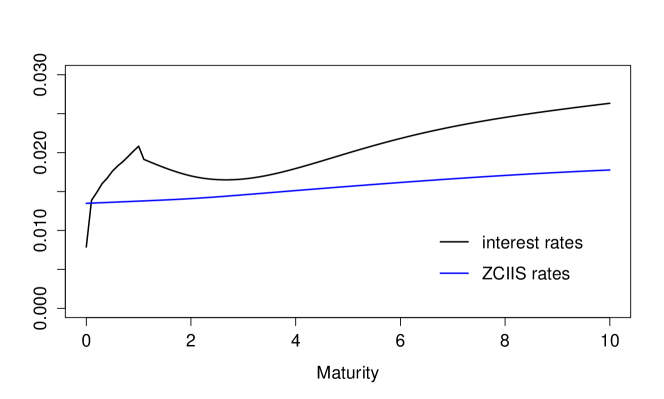
Figure 1: Yield curve and ZCIIS curve from September, 29th 2011

We fixed the time horizon $T=10$ and chose the parameters of the common CIR process as $\lambda=0.026,\theta=0.65,\eta=0.5,x=3.45$. The $M$ individual driving processes are chosen to be CIR processes with added jumps (see appendix, equation (25)). Their parameters and the parameters $\overline{u}_{k}$ are calibrated with the mentioned recursive method. In each step the parameters are chosen so that the mean squared errors of implied volatilities are minimized. In contradiction with Grbac et al. [9] we were not able to produce a similar calibration quality as described in their paper. The resulting calibration can be found in figure 2. Especially for long dated caplet volatilities the pronounced skew could not be reproduced. Nevertheless the model provides a reasonable fit of the caplet volatility surface, especially since the focus is on inflation derivatives.

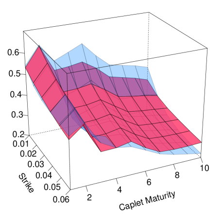
Figure 2: Market and model caplet implied volatilities of 6-month forward interest rates with strikes $1\%$ to $6\%$ and maturities from 1 to 10 years. Market volatilities are in a transparent blue, while model volatilities are displayed in red.

The next step is to extend the calibration to inflation markets. Additionally to the $M+1$ driving processes used for modeling interest rates we use another $M$ independent analytic affine processes (one for each year) driving inflation-related quantities. Since the individual processes are independent by (23) the setup without inflation can be embedded by setting the additional components of $u_{k}$ equal to zero (see table 1). So from now on we assume that the processes $X^{0},X^{1},\dots,X^{M}$ and the vectors $u_{1},\dots,u_{N}$ are already fixed.

The choice of the inflation parameters $v_{k}$ focuses on the same aspects aspects as the choice of $u_{k}$ without the restriction that inflation rates have to be nonnegative. We again assume that the vectors $v_{k}$ are determined by $2N$ parameters $\tilde{v}_{1},\dots,\tilde{v}_{N}$, $\overline{v}_{1},\dots,\overline{v}_{N}.$ In particular, we choose (see also table 2)

	$X^{0}$	$X^{1}$	$X^{2}$	…	$X^{M}$	$X^{M+1}$	$X^{M+2}$	…	$X^{2M}$
$v_{1}$	$\tilde{v}_{1}$	$\overline{u}_{1}$	$\overline{u}_{3}$	$\dots$	$\overline{u}_{N-1}$	$\overline{v}_{1}$	$0$	$\cdots$	$0$
$v_{2}$	$\tilde{v}_{2}$	$\overline{u}_{2}$	$\overline{u}_{3}$	$\dots$	$\overline{u}_{N-1}$	$\overline{v}_{2}$	$0$	$\cdots$	$0$
$v_{3}$	$\tilde{v}_{3}$	0	$\overline{u}_{3}$	$\dots$	$\overline{u}_{N-1}$	$0$	$\overline{v}_{3}$	$\cdots$	$0$
$v_{4}$	$\tilde{v}_{4}$	0	$\overline{u}_{4}$	$\dots$	$\overline{u}_{N-1}$	$0$	$\overline{v}_{4}$	$\cdots$	$0$
⋮	⋮	⋮	⋮	$\ddots$	⋮	⋮	⋮	$\ddots$	⋮
$v_{N-2}$	$\tilde{v}_{N-2}$	0	0	$\dots$	$\overline{u}_{N-1}$	$0$	0	$\cdots$	0
$v_{N-1}$	$\tilde{v}_{N-1}$	0	0	$\dots$	$\overline{u}_{N-1}$	$0$	0	$\cdots$	$\overline{v}_{N-1}$
$v_{N}$	$\tilde{v}_{N}$	0	0	$\dots$	$\overline{u}_{N}$	$0$	0	$\cdots$	$\overline{v}_{N}$

Table 2: Description of the inflation parameter structure $v_{k}$. Each row corresponds to one vector with the column names denoting the process the position in the vector corresponds to. Note that for annual inflation rate option pricing the vectors $v_{j}$ with $j$ odd do not matter.

$$v_{k}=\tilde{v}_{k}\mathrm{e}^{0}+\overline{u}_{k}e^{\left\lceil\frac{k}{2}\right\rceil}+\sum_{l=\left\lceil\frac{k}{2}\right\rceil+1}^{M}\overline{u}_{2l-1}e^{l}+\overline{v}_{k}e^{M+\left\lceil\frac{k}{2}\right\rceil}.$$

Choosing the nominal components $v_{k}^{i}=u_{k}^{i}$ for $i=1,\dots,M$ has the advantage that forward CPIs and therefore also forward inflation rates do not depend on the nominal processes $X^{1},\dots,X^{M}$. Together with the choice of $v_{k}$ with respect to the inflation processes $X^{M+1},\dots X^{2M}$ this implies that the forward CPI $\operatorname{\mathcal{I}}(t,T_{2k})$ depends only on $X^{0}$ and $X^{M+k}$. In particular the function $B(t,v_{2k},u_{2k})$ corresponding to the forward CPI $\operatorname{\mathcal{I}}(t,T_{2k})$ defined in (11) is

$$B(t,v_{2k},u_{2k}) =(\psi_{T-t}^{0}(\tilde{v}_{2k})-\psi_{T-t}^{0}(\tilde{u}_{2k}),0,\dots,0,\psi_{T-t}^{M+k}(\overline{v}_{2k}),0,\dots,0).$$

From this it follows that for different forward CPIs these functions are “orthogonal” except for the first component. Furthermore except for the first component they are also “orthogonal” to the functions $B(t,u_{j-1},u_{j})$ relevant for forward interest rates. Hence the correlation structure mainly depends on $\tilde{u}_{k}$ and $\tilde{v}_{k}$. Since $\psi_{t}^{0}$ is monotonically increasing, one should choose $\tilde{v}_{k}>\tilde{u}_{k}$ if the corresponding forward CPI should be positively correlated with nominal interest rates or $\tilde{v}_{k}<\tilde{u}_{k}$ if it should be negatively correlated. Also note that two annual forward CPIs are positively correlated if $\,\mathrm{sgn}\left(\tilde{v}_{k}-\tilde{u}_{k}\right)=\,\mathrm{sgn}\left(\tilde{v}_{j}-\tilde{u}_{j}\right)$. This therefore gives us some criteria how to determine the parameters $\tilde{u}_{k}$ from correlation assumptions and from now on we assume that the parameters $\tilde{v}_{1},\dots,\tilde{v}_{N}$ are given. Assuming also a fixed process $X^{M+k}$ we would like to determine $\overline{v}_{k}$ from the current term structure $P_{ILB}(0,T_{k})/P(0,T)$. We differentiate between two cases. First consider a nonnegative affine process $X^{M+k}$. In this case by Lemma 2 there exists a unique $\overline{v}_{k}$, so that $M_{0}^{v_{k}}=P_{ILB}(0,T_{k})/P(0,T)$. For $\tilde{v}_{k}\approx\tilde{u}_{k}$ this typically results in $\overline{v}_{k}>0$. In this case zero coupon inflation for $[t,T_{k}]$ is always positive. To avoid this alternatively consider an affine process, which takes negative and positive values. In this case $M_{0}^{v}$ is not necessarily increasing in $\overline{v}_{k}$. However, by Lemma 2 it is still a convex function in $\overline{v}_{k}$. This means that there are at most two possible choices for $\overline{v}_{k}$, in which case we need to pick one. For the results in this paper we only used results where one choice was smaller than zero and the other one larger than zero, which we then picked. To determine the processes $X^{M+1},\dots,X^{2M}$ notice that the annual forward inflation rate $F_{I}(t,T_{2k-2},T_{2k})$ depends only the processes $X^{0},X^{M+k-1},X^{k}$ and $F_{I}(t,T_{0},T_{2})$ depends only on $X^{0},X^{M+1}$. By starting with inflation options on $F_{I}(T_{2},T_{0},T_{2})$ one can calibrate the parameters of $X^{M+1}$. Then one can iteratively calibrate the parameters of $X^{M+k}$ using inflation options on $F_{I}(T_{2k},T_{2(k-1)},T_{2k})$.

For the calibration example we used ZCIIS rates from $1$ to $10$ years (see figure 1) and inflation options for strikes ranging from $-2\%$ to $6\%$, the prices of which are displayed in figure 4. We chose $\tilde{v}_{k}=\tilde{u}_{k}(1+ck)$ with $c\approx 0.08$, so that $ck$ is between $1$ and $1.15$. This means that correlation are positive as usually observed. For the processes $X^{M+1},\dots,X^{2M}$ we used Ornstein-Uhlenbeck processes with added jumps (see appendix, equation (26)). The parameters of these processes and the sequence $(\overline{v}_{k})$ are then calibrated as described. In each step the mean squared errors of option prices are minimized. The resulting fit is displayed in figure 4 and this shows that the calibration is very accurate.

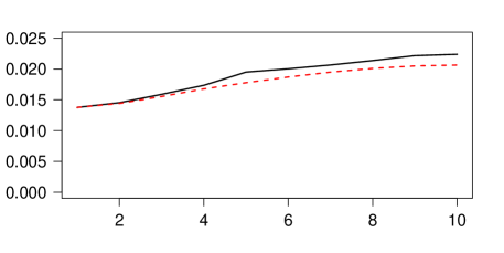
Figure 3: Linear interpolated annual forward inflation rates $F_{I}(0,T_{2(k-1)},T_{2k})$ (black) and its approximation $\operatorname{\mathcal{I}}(t,T_{2k})/\operatorname{\mathcal{I}}(t,T_{2(k-1)})-1$ (dashed red) for maturities from 1 to 10 years.

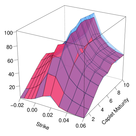
Figure 4: Market and model caplet/floorlet prices in basis points for annual forward inflation with strikes $-2\%$ to $6\%$ and maturities from 1 to 10 years. Market prices are in a transparent blue, while model prices are displayed in red. For strikes between $-2\%$ and $1\%$ prices are quoted for floorlets, for strikes between $2\%$ and $6\%$ prices are quoted for caplets. Market prices are bootstrapped from corresponding cap/floor data.

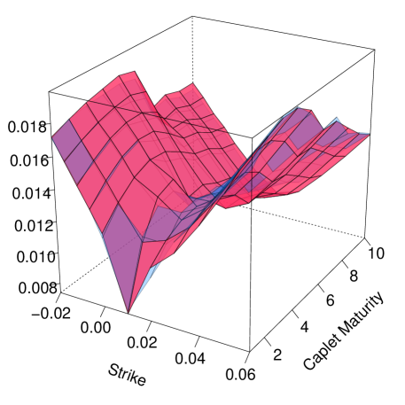
Figure 5: Market and model implied volatilities for annual forward inflation with strikes $-2\%$ to $6\%$ and maturities from 1 to 10 years. Market volatilities are in a transparent blue, while model volatilities are displayed in red.

We would also like to display the fit in terms of (shifted lognormal) implied volatilities. Typically one only has quotes on ZCIIS rates, which do not directly translate to forward inflation rates. However, annual forward inflation rates can be approximated by $F_{I}(t,T_{k-j},T_{k})\approx\operatorname{\mathcal{I}}(t,T_{k})/\operatorname{\mathcal{I}}(t,T_{k-j})-1$ (see figure 3). It is market practice to use this as forward value in the shifted Black formula to calculate approximate market volatilities. The resulting fit in terms of shifted implied volatilities is then displayed in figure 5. This shows that implied volatilities are closely reproduced by the model across all maturities and smiles and that the model is very capable in fitting the observed market data.

Conclusion

We have introduced a highly tractable inflation market model, where we are able to derive analytical formulas for both types of inflation-indexed swaps. Furthermore inflation caps and floors as well as CPI caps and floors can be calculated with a one-dimensional Fourier inversion formula. Hence prices for liquidly traded inflation derivatives can be calculated quickly and accurately. Additionally the proposed model is able to price classical interest rate derivatives like caps and floors. Using these formulas we are able to calibrate the model to market data. The calibration example shows that the model can be calibrated to inflation market data very accurately.

Appendix A Affine processes

Let $X=(X_{t})_{0\leq t\leq T}$ be a homogeneous Markov process with values in $D=\operatorname{\mathbb{R}}^{m}_{\geq 0}\times\operatorname{\mathbb{R}}^{n}$ on a measurable space $(\Omega,\mathcal{A})$ with filtration $(\operatorname{\mathcal{F}}_{t})_{0\leq t\leq T}$, with regards to which $X$ is adapted. Denote by $\operatorname{\mathbb{P}}^{x}$ and $\mathbb{E}^{x}\left[\cdot\right]$ the corresponding probability and expectation when $X_{0}=x$. X is said to be an affine process, if its characteristic function has the form

$$\mathbb{E}^{x}\left[\mathrm{e}^{u\cdot X_{t}}\right]=\,\mathrm{exp}\Big{(}\phi_{t}(u)+\psi_{t}(u)\cdot x\Big{)},\quad u\in{\mathbf{\mathfrak{i}}}\operatorname{\mathbb{R}}^{d},x\in D,$$

where $\phi:[0,T]\times{\mathbf{\mathfrak{i}}}\operatorname{\mathbb{R}}^{d}\rightarrow\operatorname{\mathbb{C}}$ and $\psi:[0,T]\times{\mathbf{\mathfrak{i}}}\operatorname{\mathbb{R}}^{d}\rightarrow\operatorname{\mathbb{C}}^{d}$ and ${\mathbf{\mathfrak{i}}}\operatorname{\mathbb{R}}^{d}=\{u\in\operatorname{\mathbb{C}}^{d}:\mathrm{Re}(u)=0\}.$ By homogeneity and the Markov property the conditional characteristic function satisfies

$$\mathbb{E}^{x}\left[e^{u\cdot X_{t}}|\operatorname{\mathcal{F}}_{s}\right]=\,\mathrm{exp}\Big{(}\phi_{t-s}(u)+\psi_{t-s}(u)\cdot X_{s}\Big{)}.$$ (18)

Accordingly affine processes can also be defined for inhomogeneous Markov processes (see Filipovic [6]). In this case the affine property reads

$$\mathbb{E}^{x}\left[\mathrm{e}^{u\cdot X_{t}}|\operatorname{\mathcal{F}}_{s}\right]=\,\mathrm{exp}\Big{(}\phi_{s,t}(u)+\psi_{s,t}(u)\cdot X_{s}\Big{)},\quad u\in{\mathbf{\mathfrak{i}}}\operatorname{\mathbb{R}}^{d},x\in D,$$

with $\phi_{s,t}:{\mathbf{\mathfrak{i}}}\operatorname{\mathbb{R}}^{d}\rightarrow\operatorname{\mathbb{C}}$ and $\psi_{s,t}:{\mathbf{\mathfrak{i}}}\operatorname{\mathbb{R}}^{d}\rightarrow\operatorname{\mathbb{C}}^{d}$ for $0\leq s\leq t$.

$X$ is called an analytic affine process, if $X$ is stochastically continuous and the interior of the set

$$\mathcal{V} :=\left\{u\in\operatorname{\mathbb{C}}^{d}:\sup_{0\leq s\leq T}\mathbb{E}^{x}\left[\mathrm{e}^{\mathrm{Re}(u)\cdot X_{s}}\right]<\infty\quad\forall x\in D\right\},$$ (19)

contains 0. In this case the functions $\phi$ and $\psi$ have continuous extensions to $\mathcal{V}$, which are analytic in the interior, such that (18) holds for all $u\in\mathcal{V}$ (see Keller-Ressel [11]).

The class of affine processes includes Brownian motion and more generally all Lévy processes. Since Lévy processes have stationary independent increments, it follows that $\psi_{t}(u)=u$, while $\phi_{t}(u)=t\kappa(u)$, where $\kappa$ is the cumulant generating function of the Lévy process. Ornstein-Uhlenbeck processes are further important examples of affine processes. The affine processes used in this work are described at the end of this section.

The standard reference for affine processes is Duffie et al. [4]. There they give a characterization of affine processes, where $\phi$ and $\psi$ are specified as solutions of a system of differential equations. To motivate this consider an affine process $X$. By the tower property for conditional expectations it holds for all $x\in D$

$$\mathbb{E}^{x}\left[e^{uX_{t+s}}\right]=\mathbb{E}^{x}\left[\mathbb{E}^{x}\left[e^{uX_{t+s}}|\operatorname{\mathcal{F}}_{s}\right]\right]=\mathbb{E}^{x}\left[e^{\phi_{t}(u)+\psi_{t}(u)\cdot X_{s}}\right].$$

Using equation (18) it follows that $\phi$ and $\psi$ satisfy the so-called semi-flow equations

$$\phi_{t+s}(u) =\phi_{t}(u)+\phi_{s}(\psi_{t}(u)),\qquad \phi_{0}(u) =0,$$ (20)

$$\psi_{t+s}(u) =\psi_{s}(\psi_{t}(u)), \psi_{0}(u) =u.$$

For a stochastically continuous affine process $X$ it was shown in Keller-Ressel et al. [13] that the functions

$$F(u):=\left.\frac{\partial}{\partial t}\phi_{t}(u)\right|_{t=0^{+}},\qquad R(u):=\left.\frac{\partial}{\partial t}\psi_{t}(u)\right|_{t=0^{+}}$$

exist. Rewriting (20) in terms of difference quotients and letting $s\rightarrow 0$ we get that $\phi$ and $\psi$ satisfy generalized Ricatti equations

$$\frac{\partial}{\partial t}\phi_{t}(u) =F(\psi_{t}(u)),\qquad\phi_{0}(u)=0,$$ (21)

$$\frac{\partial}{\partial t}\psi_{t}(u) =R(\psi_{t}(u)),\qquad\phi_{0}(u)=u.$$

The functions $F$ and $R$ have a specific form of Levy-Khintchine type as first described in Duffie et al. [4]. There it is also shown that for every $F$ and $R$ of this form (21) has a unique solution. Specifying the functions $F$ and $R$ is an alternative way to specify an affine process. Keller-Ressel and Mayerhofer [12] give conditions on $F$ and $R$ under which a solution of (21) defines an analytic affine process. Note that in order to evaluate $\phi$ and $\psi$ one would like to have closed form solutions to the system (21), which in general is not the case.

Coupling independent affine processes is very tractable. For two independent affine processes $X$ and $Y$ and all starting values $x,y$ one obtains

$$\mathbb{E}^{(x,y)}\left[\mathrm{e}^{(u_{X},u_{Y})\cdot(X_{t},Y_{t})}\right]=\mathbb{E}^{(x,y)}\left[\mathrm{e}^{u_{X}\cdot X_{t}}\mathrm{e}^{u_{Y}\cdot Y_{t}}\right]=\mathbb{E}^{(x,y)}\left[\mathrm{e}^{u_{X}\cdot X_{t}}\right]\mathbb{E}^{(x,y)}\left[\mathrm{e}^{u_{Y}\cdot Y_{t}}\right].$$ (22)

Hence $(X,Y)$ is an affine process with

$$\phi^{(X,Y)}_{t}(u_{X},u_{Y}) =\phi_{t}^{X}(u_{X})+\phi_{t}^{Y}(u_{Y}),$$ (23)

$$\psi^{(X,Y)}_{t}(u_{X},u_{Y}) =(\psi_{t}^{X}(u_{X}),\psi_{t}^{Y}(u_{Y})).$$

This fact together with the following Lemma is used in section 3.

Lemma 2.

Let $X$ be an analytic affine processes comprised of $m+n$ independent affine processes, where the first $m$ are nonnegative. For $(u_{1},\dots,u_{k},v,u_{k+1},\dots,u_{n})\in\mathrm{int}(\mathcal{V})\cap\operatorname{\mathbb{R}}^{m+n}$ define the function

$$f^{k}(v):=\mathbb{E}^{x}\left[\mathrm{e}^{(u_{1},\dots,u_{k-1},v,u_{k+1},\dots,u_{m+n})\cdot X_{t}}\right].$$

Then $f^{k}$ is monotonically increasing if $k\leq m$ and $f^{k}$ is convex for all $k$.

Proof.

For each $x\in D$ the term inside the expectation is convex in $v$ and monotonically increasing in $v$ if $k\leq m$. This then also holds after taking the expectation. ∎

The last part of this section describes the affine processes used in this paper. One classical example is the CIR process, which is the unique solution of

$$\,\mathrm{d}X_{t}=-\lambda(X_{t}-\theta)\,\mathrm{d}t+2\eta\sqrt{X_{t}}\,\mathrm{d}W_{t},\qquad X_{0}=x.$$ (24)

For this process the functions $\phi$ and $\psi$ are defined for $\mathrm{Re}(u)<\frac{\lambda}{2\eta^{2}}(1-\mathrm{e}^{-\lambda t})^{-1}$,

$$\phi_{t}(u) =-\frac{\lambda\theta}{2\eta^{2}}\,\ln\left(1-\frac{2\eta^{2}}{\lambda}(1-\mathrm{e}^{-\lambda t})u\right),$$

$$\psi_{t}(u) =\frac{\mathrm{e}^{-\lambda t}u}{1-\frac{2\eta^{2}}{\lambda}(1-\mathrm{e}^{-\lambda t})u}.$$

The CIR process almost surely stays nonnegative. It is strictly positive if $\frac{\lambda\theta}{2}>\eta^{2}$. One can add jumps to this process by adding the differential of a compound Poisson process $L_{t}$ to the dynamics of $X$.

$$\,\mathrm{d}X_{t}=-\lambda(X_{t}-\theta)\,\mathrm{d}t+2\eta\sqrt{X_{t}}\,\mathrm{d}W_{t}+\,\mathrm{d}L_{t},\qquad X_{0}=x.$$ (25)

If $L_{t}$ has exponentially distributed jumps with expectation values $\frac{1}{\alpha}$ arriving at rate $\lambda\beta$ the functions $\phi$ and $\psi$ are (see Grbac and Papapantoleon [8])

$$\phi_{t}(u) =-\frac{\lambda\theta}{2\eta^{2}}\,\ln\left(1-\frac{2\eta^{2}}{\lambda}(1-\mathrm{e}^{-\lambda t})u\right)-\frac{\lambda\beta}{\lambda-2\eta^{2}\alpha}\,\ln\left(\frac{\alpha-u}{\alpha-u\left(\mathrm{e}^{-\lambda t}+(1-\mathrm{e}^{-\lambda t})\frac{1}{\lambda}2\eta^{2}\alpha\right)}\right),$$

$$\psi_{t}(u) =\frac{\mathrm{e}^{-\lambda t}u}{1-\frac{2\eta^{2}}{\lambda}(1-\mathrm{e}^{-\lambda t})u},$$

where

$$\mathrm{Re}(u)<\min\left\{\frac{\lambda}{2\eta^{2}}(1-\mathrm{e}^{-\lambda t})^{-1},\alpha\left(\mathrm{e}^{-\lambda t}+(1-\mathrm{e}^{-\lambda t})\frac{1}{\lambda}2\eta^{2}\alpha\right)^{-1},\alpha\right\}.$$

Since $L_{t}$ has only positive jumps this process also stays nonnegative. As a third example consider the real-valued affine process defined by

$$\,\mathrm{d}X_{t}=-\lambda(X_{t}-\theta)\,\mathrm{d}t+\sigma\,\mathrm{d}W_{t}+\,\mathrm{d}\tilde{L}_{t},\qquad X_{0}=x,$$ (26)

where $\tilde{L}_{t}$ is a compound Poisson process with positive jumps with mean $\frac{1}{\alpha^{+}}$ arriving at rate $\lambda\beta^{+}$ and negative jumps with mean $\frac{1}{\alpha^{-}}$ arriving at rate $\lambda\beta^{-}$. The functions $\phi$ and $\psi$ in this case read (see Müller and Waldenberger [19])

$$\phi_{t}(u) =\frac{\sigma^{2}u^{2}}{4\lambda}(1-\mathrm{e}^{-2\lambda t})+\theta u(1-\mathrm{e}^{-\lambda t})+\frac{\beta^{+}+\beta^{-}}{2}\,\ln\left(\frac{(\alpha^{+}-\mathrm{e}^{-\lambda t}u)(\alpha^{-}+\mathrm{e}^{-\lambda t}u)}{(\alpha^{+}-u)(\alpha^{-}+u)}\right)$$

$$+\frac{\beta^{+}-\beta^{-}}{2}\,\ln\left(\frac{(\alpha^{+}-\mathrm{e}^{-\lambda t}u)(\alpha^{-}+u)}{(\alpha^{+}-u)(\alpha^{-}+\mathrm{e}^{-\lambda t}u)}\right),$$

$$\psi_{t}(u) =\mathrm{e}^{-\lambda t}u,$$

for $-\alpha^{-}<\mathrm{Re}(u)<\alpha^{+}$.

Graz University of Technology, Institute of Statistics, NAWI Graz

Kopernikusgasse 24/III, 8010 Graz, Austria

E-mail address: stefan.waldenberger@tugraz.at

References

- Belgrade et al. [2004] N. Belgrade, E. Benhamou, and E. Koehler. A Market Model for Inflation. SSRN eLibrary, 2004.
- [2] A. Brace, D. Gatarek, and M. Musiela. The market model of interest rate dynamics. Mathematical Finance, 7(2). ISSN 1467-9965.
- Cuchiero and Teichmann [2013] C. Cuchiero and J. Teichmann. Path properties and regularity of affine processes on general state spaces. In Séminaire de Probabilités XLV, Lecture Notes in Mathematics, pages 201–244. Springer International Publishing, 2013.
- Duffie et al. [2003] D. Duffie, D. Filipović, and W. Schachermayer. Affine processes and applications in finance. Annals of Applied Probability, 13:984–1053, 2003.
- Eberlein et al. [2010] E. Eberlein, K. Glau, and A. Papapantoleon. Analysis of fourier transform valuation formulas and applications. Applied Mathematical Finance, 17(3):211–240, 2010.
- Filipovic [2005] D. Filipovic. Time-inhomogeneous affine processes. Stochastic Processes and their Applications, 115(4):639–659, 2005.
- Fleckenstein et al. [2010] M. Fleckenstein, F. A. Longstaff, and H. N. Lustig. Why Does the Treasury Issue TIPS? The TIPS-Treasury Bond Puzzle. SSRN eLibrary, 2010.
- Grbac and Papapantoleon [2013] Z. Grbac and A. Papapantoleon. A tractable libor model with default risk. Mathematics and Financial Economics, 7(2):203–227, 2013. ISSN 1862-9679.
- Grbac et al. [2014] Z. Grbac, A. Papapantoleon, J. Schoenmakers, and D. Skovmand. Affine LIBOR models with multiple curves: theory, examples and calibration. ArXiv e-prints, May 2014.
- Jarrow and Yildirim [2003] R. Jarrow and Y. Yildirim. Pricing treasury inflation protected securities and related derivatives using an HJM model. Journal of Financial and Quantitative Analysis, 38(2):337–359, 2003.
- Keller-Ressel [2008] M. Keller-Ressel. Affine processes - Theory and application in finance. PhD-thesis, Wien University of Technology, 2008.
- Keller-Ressel and Mayerhofer [2011] M. Keller-Ressel and E. Mayerhofer. Exponential moments of affine processes. ArXiv e-prints, Nov. 2011.
- Keller-Ressel et al. [2001] M. Keller-Ressel, J. Teichmann, and W. Schachermayr. Affine processes are regular. Journal of Probability Theory and Related Fields, 151(3-4):591–611, 2001.
- Keller-Ressel et al. [2013a] M. Keller-Ressel, A. Papapantoleon, and J. Teichmann. The affine LIBOR models. Mathematical Finance, 23(4):627–658, 2013a.
- Keller-Ressel et al. [2013b] M. Keller-Ressel, W. Schachermayer, and J. Teichmann. Regularity of affine processes on general state spaces. Electron. J. Probab., 18:no. 43, 1–17, 2013b.
- Mercurio [2005] F. Mercurio. Pricing inflation-indexed derivatives. Journal of Quantitative Finance, 5(3):289–302, 2005.
- Mercurio and Moreni [2006] F. Mercurio and N. Moreni. Inflation with a smile. Risk magazine, 2006.
- Mercurio and Moreni [2009] F. Mercurio and N. Moreni. A multi-factor SABR model for forward inflation rates. SSRN eLibrary, 2009.
- Müller and Waldenberger [2015] W. Müller and S. Waldenberger. Affine LIBOR models driven by real-valued affine processes. arXiv:1503.00864, 2015.