Gas inside the 97 au cavity around the transition disk Sz 91

Abstract

We present ALMA (Cycle 0) band-6 and band-3 observations of the transition disk Sz 91. The disk inclination and position angle are determined to be $i=49.5\arcdeg\pm 3.5\arcdeg$ and $\mathrm{PA}=18.2\arcdeg\pm 3.5\arcdeg$ and the dusty and gaseous disk are detected up to $\sim 220$ au and $\sim 400$ au from the star, respectively. Most importantly, our continuum observations indicate that the cavity size in the mm-sized dust distribution must be $\sim 97$ au in radius, the largest cavity observed around a T Tauri star. Our data clearly confirms the presence of ${}^{12}\mathrm{CO}$ (2-1) well inside the dust cavity. Based on these observational constrains we developed a disk model that simultaneously accounts for the ${}^{12}\mathrm{CO}$ and continuum observations (i.e., gaseous and dusty disk). According to our model, most of the millimeter emission comes from a ring located between 97 and 140 au. We also find that the dust cavity is divided into an innermost region largely depleted of dust particles ranging from the dust sublimation radius up to 85 au, and a second, moderately dust-depleted region, extending from 85 to 97 au. The extremely large size of the dust cavity, the presence of gas and small dust particles within the cavity and the accretion rate of Sz 91 are consistent with the formation of multiple (giant) planets.

1 Introduction

Simulations of disk-planet interactions show that a giant planet embedded in a circumstellar disk should open a gap or carve an inner hole in the disk (Lin & Papaloizou, 1986). These gaps or holes are imprinted in the spectral energy distributions (SEDs) of young stellar objects as reduced near and/or mid infrared excess emission. Protoplanetary disks showing this observational feature are usually called “transition disks”, although different names and classifications are found in the literature (Evans et al., 2009). Apart from planet formation, three alternative mechanisms can create opacity holes in the inner disk: grain growth (Dullemond & Dominik, 2005), photoevaporation (Alexander et al., 2006), and tidal truncation by close stellar companions (Artymowicz & Lubow, 1994).

The latest models of photoevaporation show that only transition disks with small accretion rates and/or small inner cavities can be explained by this process (Owen et al., 2012). While grain growth and transport effects can explain the dips in the SEDs of transition disks, the most recent models fail in reproducing the large cavities observed in millimeter images of accreting transition disks (Birnstiel et al., 2013). Current planet formation models predict that a forming planet may reduce (or remove if the planet is massive enough) the amount of small particles within the disk’s cavity while allowing the gas to flow through the cavity (e.g., Rice et al., 2006; Lubow & D’Angelo, 2006; Dodson-Robinson & Salyk, 2011; Zhu et al., 2011).

The transition disk Sz 91, at 200 pc (Merín et al., 2008), has been classified as a planet forming candidate based on its lack of detected companions down to 30 au, its disk mass, accretion rate ($7.9\times 10^{-11}\mathrm{M_{\sun}}\,\mathrm{yr}^{-1}$), and SED shape (Romero et al., 2012). Recently, Tsukagoshi et al. (2014) (hereafter T2014) resolved the inner cavity in K-band polarized light with Hi CIAO/Subaru, and find evidences for a gap in the continuum at 345 GHz (870 µm) from SMA observations. These authors also detect the outer gaseous disk using the ${}^{12}\mathrm{CO}(3-2)$ line. We here use ALMA cycle 0 band-6 and band-3 observations to describe the disk in more detail. Our observations reveal a huge cavity of $\sim$97 au in radius in the continuum at 230 GHz (1.3 mm), and confirm the presence of ${}^{12}\mathrm{CO}(2-1)$ inside the cavity. We also derive stronger constrains on the disk’s geometry and orientation.

2 Observations and Data reduction

Table 1: Observing log.

LO	Date	Flux	$\tau_{\nu}$	PWV	$\mathrm{t_{exp}}$	$\mathrm{T_{sys}}$	bandwidth
$\mathrm{[GHz]}$	[dd/mm/yy]	Calibrator	Zenith	[mm]	[min]	[K]	[GHz]
231.46	18/06/2012	Titan	0.09	1.586	3.77	96	$2\times$1.875
231.46	02/07/2012	Neptune	0.05	0.827	3.77	70	$2\times$1.875
231.46	03/07/2012	Neptune	0.08	1.520	3.77	79	$2\times$1.875
231.46	04/07/2012	Titan	0.10	1.877	3.77	82	$2\times$1.875
109.99	01/08/2012	Neptune	0.03	1.552	0.4	53	$4\times$1.875

2.1 Interferometry

Sz 91 was observed with ALMA band-6 (231 GHz) and band-3 (110 GHz) during Cycle-0 (program 2011.0.00733, PI: M.R. Schreiber). The observations are summarized in Table 1.

Sz 91 was observed in five different epochs with different weather conditions and antenna configurations for the band-6 data. The system temperature ranged from 53 to 96 K. For the band-3 data, the ALMA correlator was configured to provide two spectral windows centered on the continuum, and two spectral windows centered on the ${}^{13}\rm{CO(1-0)}$ (110.20135 GHz) and the $\rm{C^{18}O(1-0)}$ (109.78218 GHz) lines. The total bandwidth of the band-3 observations was 7.5 GHz ($4\times 1.875$ GHz). For the band-6 observations, the ALMA correlator was initially configured to provide 1 spectral window centered on the continuum, and three spectral windows centered on the ${}^{12}\mathrm{CO}(2-1)$, 230.538 GHz (hereafter ${}^{12}\mathrm{CO}$ ), ${}^{13}\mathrm{CO}(2-1)$ and $\mathrm{C^{18}O}(2-1)$ lines. Unfortunately, because of technical problems only one sideband of the correlator could be configured, and only the spectral windows centered on the continuum and on the ${}^{12}\mathrm{CO}$ line could be produced. The total bandwidth of the band-6 observations was $2\times 1.875$ GHz. Both ALMA bands were sampled at 0.488 MHz (e.g., 0.635 km/s in the ${}^{12}\mathrm{CO}$ line).

The quasar QSO B1730-130 and the AGN ICRF J160431.0-444131 were used as bandpass and primary phase calibrator in both bands, respectively. Neptune and Titan were used to calibrate in amplitude in band-3 and band-6, respectively. The observations of the calibrators were alternated with the science observations. The individual exposure times for the calibrators and the science targets was 6.05 seconds, amounting to a total exposure time for the science observations of 226 seconds (3.77 minutes) in band-6 and 24 seconds (0.4 minutes) in band-3. Phase correction based on WVR measurements was performed in offline mode, as part of the basic ALMA Cycle 0 corrections. We used the dispersion of the band-6 flux calibrations to estimate a flux uncertainty of $\approx 15\%$. This value is a lower limit since it does not include uncertainties from the amplitude calibration.

The observations were processed using the Common Astronomy Software Application (CASA) package (McMullin et al., 2007). The visibilities were Fourier transformed and deconvolved, using natural weighting, with the CLEAN algorithm (Högbom, J. A., 1974). For the band-6 data, we combined the four datasets to increase the $uv$ coverage before cleaning. The cleaned image produced from this concatenated dataset had lower rms than the images created from individually cleaned datasets. After combining the band-6 data, the two bands contained 276 baselines, ranging from 21 to 402 m (16 to 309 k$\lambda$) in band-6, and from 21 to 452 m (7 to 167 k$\lambda$) in band-3.

In the continuum, we reach a rms of 0.1 mJy/beam in band-6 and 0.1 mJy/beam in band-3. The median rms on the channels associated to the ${}^{12}\mathrm{CO}$ , is 6.2 mJy/beam. In the continuum, the beam is $0\farcs 86\times 0\farcs 60$ with a position angle (PA) of $88.9\arcdeg$ in band-6, and $2\farcs 08\times 1\farcs 51$ with a PA of $99.4\arcdeg$ in band-3. No emission was detected in either the ${}^{13}\mathrm{CO}(1-0)$ or the $\mathrm{C^{18}O}(1-0)$ lines in band-3.

2.2 Photometry

We add two WISE flux at 12 and 22 µm, two Herschel/PACS fluxes at 100 and $160\micron$, three Herschel/Spire fluxes at 250, 350 and $500\micron$ and the two mm-fluxes discussed here to the photometry presented by Romero et al. (2012). For the Herschel fluxes we adopt the most recent values presented by Bustamante et al. (2015). The fluxes at wavelengths shorter than 24 $\micron$ were corrected of extinction by applying the dereddening relations listed in Cieza et al. (2007). We assume calibration errors of 20% for the optical photometry and 15% for the photometry up to 24µm. The photometry between 100-500 $\micron$ is affected by background contamination from the cloud in which Sz 91 is embedded, specially at 250, 350 and 500 $\micron$ (Bustamante et al., 2015). We therefore consider the Herschel fluxes at 250, 350 and 500 as upper limits. For the 870$\micron$ flux we used the $8.5\%$ uncertainty listed by Romero et al. (2012). To derive the fluxes from our ALMA observations we perform a fit in the $uv$-plane. Because of the lack of data at short baselines (i.e., large spatial scales), deriving the total flux from the cleaned images would result in underestimated values. Instead we fit different profiles to the visibilities to estimate the flux at the center of the $uv$-plane. In band-6 Sz 91 is resolved (see next section), so we fit a Gaussian profile; in band-3 Sz 91 is not resolved, so we use a point-source profile. The fluxes comprising the SED, their errors and references, are listed in Table 2.

Table 2: Photometry of Sz 91. All fluxes are extinction-corrected. References: (1) Romero et al. (2012), (2) Wright et al. (2010). (3) Merín et al. (2008), (4) Bustamante et al. (2015)

Wavelength	Flux	Error	Reference
$[\mu$m]	[mJy]	[mJy]
0.65	37.1	7.4	1
1.25	97.7	14.7	1
1.60	120.6	18.1	1
2.20	90.6	13.6	1
3.60	41.6	6.2	1
4.50	26.0	3.9	1
5.60	17.8	2.7	1
8.00	11.1	1.7	1
12.00	6.9	1.0	2
22.00	9.0	1.4	2
24.00	9.7	1.5	3
70.00	510.0	130.0	4
100.00	680.0	170.0	4
160.00	720.0	180.0	4
250.00	860.0	170.0	4
350.00	620.0	120.0	4
500.00	380.0	80.0	4
850.00	34.5	2.9	1
1300.00	12.7	1.9	This work
2700.00	0.7	0.1	This work

3 Continuum and $\mathrm{{}^{12}CO}$ images

In band-3, Sz 91 is only detected (and not resolved) in the continuum, with a maximum signal to noise ratio (S/N) of $\approx 4.6$ and a disk emission of $0.7\pm 0.1$ mJy. The median rms in the individual channels is 11.0 mJy/beam. The band-6 results are detailed below.

The continuum image (Fig. 1, left panel) shows an inclined disk (the geometry is derived in Sect. 3.3) with evidences of an inner cavity, as expected from the disk’s SED and the previous results of T2014. The inner hole is resolved along the projected major axis of the disk. Integrating over the regions of the image with S/N higher than 3 results in $\mathrm{F_{1.3mm}}=10.7\pm 1.6$ mJy, which is $\sim 20\%$ lower than the integrated flux estimated from the visibilities (see Table 2). The peak flux in the cleaned image is $3.7\pm 0.5$ mJy/beam. The difference in brightness between the peak flux of the northern and southern lobes is below 3$\sigma$.

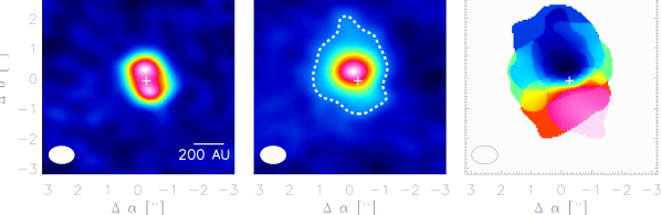
Figure 1: Left: band-6 continuum image. Center: Moment-0 image, constructed from the ${}^{12}\mathrm{CO}$ line channels showing emission above the $3\sigma$ level. The white dashed line contours the regions of the image with S/N larger than 3. The strong north-south asymmetry is most likely caused by cloud contamination (see text). Right: The moment-1 image, constructed using the same channel images as for the moment-0 image. A rotating gaseous disk is clearly identified. In all images, north is up, east is left. The white cross shows the disk’s center as derived in Sect. 4.3.

The channels corresponding to $v_{\mathrm{LSR}}$ velocities ranging from 0.5 to 4.7 km/s show significant (above $3\sigma$) ${}^{12}\mathrm{CO}$ emission (Fig. 2).

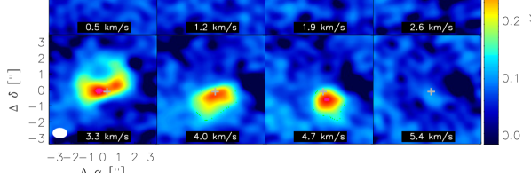
Figure 2: Band-6 channels showing significant (above $3\sigma$) ${}^{12}\mathrm{CO}$ emission. The $v_{\mathrm{LSR}}$ velocity of each channel is indicated in the legends. The channel at $v_{\mathrm{LSR}}=5.4$ km/s does not shows ${}^{12}\mathrm{CO}$ emission, and is shown for completeness. The images are plotted in square root strecht. North is up an east is left. The channel at $v_{\mathrm{LSR}}=3.3$ km/s is the closest to the derived systemic velocity of the system (see text). The grey cross shows the disk’s center as derived in Sect. 4.3.

Note that the emission at 0.5 km/s, although faint when compared to the maximum emission of the ${}^{12}\mathrm{CO}$ line, is detected with S/N $\approx 6$. The corresponding moment 0 and moment 1 images are shown in Fig. 1 (middle and right panel). The moment 0 image shows a strong north-south asymmetry, which is most likely caused by emission from the cloud in which Sz 91 is embedded. Indeed, the systemic velocity of the cloud has been measured to be $v_{\mathrm{LSR}}\approx 4.8$ km/s (Vilas-Boas et al., 2000; Tachihara et al., 2001), which coincides with the redshifted $\mathrm{{}^{12}CO}$ emission of Sz 91 (southern lobe, see the moment-1 image in Fig. 1, right panel). The same effect has been already noticed by T2014 when discussing the (less affected) ${}^{12}\rm{CO}(3-2)$ line profile. These authors estimate that the cloud affects their measurements in the range 4-7 km/s $v_{\mathrm{LSR}}$. Integrating the moment 0 image over the regions of the image with emission above $3\sigma$ (this region is delimited by the white dashed line contour in the central panel of Fig. 1) results in an integrated flux of $\mathrm{F_{{}^{12}CO}}=2.7\pm 0.4$ Jy km/s. As in the case of the continuum data, this value is an underestimation of the true flux due to the cleaning process. A Gaussian fit to the visibilities yields a larger value of $\mathrm{F_{{}^{12}CO}}=3.0\pm 0.4$ Jy km/s. Because of the cloud this value still represents a lower limit.

To determine the line center, we used public VLT/X-shooter spectra (ID: 089.C-0143) to derive the systemic radial velocity of Sz 91 (i.e., the center of the ${}^{12}\mathrm{CO}$ line) as $v_{\mathrm{LSR}}\approx 3.4\pm 0.2$ km/s, in good agreement with the results from Melo (2003) and T2014.

4 Constrains on the star and disk

In this section, we use our observations in combination with simple modeling to place constrains on some of the disk’s properties such as orientation, geometry, and mm slope. To complete our picture of the Sz 91 star$+$disk system we also derive the basic parameters of the central star.

4.1 Stellar parameters

First estimations of the Sz 91 stellar parameters were obtained by Hughes et al. (1994), who used a distance of $140\pm 20$ au, an extinction $A_{\mathrm{v}}$ of 2 and a spectral type of M0.5. These authors derived a stellar mass ranging from $M_{\star}=0.49-0.69M_{\sun}$, an effective temperature of $T_{eff}=3723$ K and an age ranging from 5-7 Myr. Romero et al. (2012) classified Sz 91 as a M1.5 star using high resolution spectra, in general agreement with the previous result. Using the latter spectral type, the most recent distance estimate of $\sim$200 pc, and an extinction of $A_{\mathrm{v}}$ = 2, we derive the stellar parameters using the stellar evolutionary models of Siess et al. (2000). We obtain a stellar radius of $R_{\star}=1.46R_{\sun}$, a temperature of $T_{eff}=3720$ K, a mass of $M_{\star}=0.47M_{\sun}$, and an age below 1 Myr. In what follows we use these values.

4.2 $\alpha_{mm}$ slope

At mm wavelengths, we can use the Rayleigh-Jeans approximation to express the flux as $F_{\nu}\propto\nu^{\alpha_{\mathrm{mm}}}$. Assuming optically thin emission, the mm-slope is a function of the dust opacity index $\beta$, i.e. $\alpha_{\mathrm{mm}}=2+\beta$. In particular, $\beta\sim 2$ for the interstellar medium (ISM) (see Williams & Cieza, 2011, and references therein). Trying to fit in this way the fluxes at 0.85, 1.3 and 2.7 mm it is not possible to match the observed fluxes, as shown in Fig. 3. The slope derived from a fit to the three fluxes results in $\alpha_{\mathrm{0.8-2.7mm}}=3.36\pm 0.14$ (solid line). Using the two shorter wavelengths we obtain $\alpha_{\mathrm{0.8-1.3mm}}=2.34\pm 0.40$ (dotted line), whereas using the fluxes at 1.3 and 2.7 mm yields to $\alpha_{\mathrm{1.3-2.7mm}}=4.07\pm 0.29$ (dashed line). This large $\alpha_{\mathrm{1.3-2.7mm}}$ would imply moderate or very low grain growth. On the other hand, our derived $\alpha_{\mathrm{0.8-1.3mm}}$ implies $\beta_{\mathrm{0.8-1.3mm}}=0.34\pm 0.40$, which suggests the opposite. This latter value agrees with the result by T2014 ($\beta=0.5\pm 0.1$) and with the average values for a set of transition disks and protoplanetary disks derived by Pinilla et al. (2014). In addition, we conclude from our models (see Sect. 5) that grains of at least 1 mm size are needed to match the SED at mm-wavelengths, implying that grain growth is happening in Sz 91 (see Sect. 5). One possible explanation of the different slopes is an optical depth effect. Enhancements in the optical thickness could reduce the slope explaining the reduction in $\alpha_{0.8-1.2mm}$ compared to the $\alpha_{1.3-2.7mm}$. However, using a sample of 50 disks, Ricci et al. (2012) find that low values of $\alpha_{mm}$ can be explained by emission from optically thick regions only in the most massive disks if their sample. Given the relatively low mass of Sz 91 (Sect. 5), the good agreement with the results by T2014, and the significant difference between $\alpha_{0.8-1.3mm}$ and $\alpha_{1.3-2.7mm}$, we consider that an underestimation of the error bars represents a more likely explanation of the broken $\alpha_{mm}$ slope and that $\alpha_{\mathrm{0.8-1.3mm}}=2.34\pm 0.40$ probably represents a realistic estimate of the true mm slope.

Figure 3: Different fits to the mm-slope ($\alpha_{mm}$). It is not possible to simultaneously match the three measurements (see text).

4.3 Disk orientation

Given the strong absorption observed towards the red-shifted channels, deriving the disk’s center and geometry by means of a Keplerian fit to the line profile as in e.g. Mathews et al. (2012) would result in large uncertainties. Instead, we determine the disk inclination ($i$), position angle (PA), and center by fitting different disk profiles to the continuum visibilities using the uvfit/MIRIAD task.

A ring morphology matches well our continuum observations and the results of T2014. Unfortunately, uvfit doesn’t allow to adjust the thickness of the fitted ring. To test for the effect of using different disk profiles, we performed three fits using a ring, a disk, and a Gaussian profile. Combining these results we derived a PA of $18.2\arcdeg\pm 3.5$ (east of north) and an inclination ($i$) of $49.5\arcdeg\pm 3.5$. These results are in agreement with those derived by T2014 ($\mathrm{PA}=17.5\arcdeg\pm 17.7\arcdeg$, $i=40\arcdeg\pm 15\arcdeg$). We find the disk’s center to have an offset of $\Delta\alpha=-0\farcs 29\pm 0\farcs 01$ and $\Delta\delta=-0\farcs 06\pm 0\farcs 02$ with respect to the center of the ALMA field. This offset is consistent with the measured proper motion of (-20.3,-18.4) mas $\mathrm{yr}^{-1}$ (UCAC3, Zacharias et al., 2010) when including the $\sim$0$\farcs$1 astrometric uncertainty from our ALMA Cycle 0 observations and the 0$\farcs$06 uncertainty from our input coordinates (2MASS catalogue, Cutri et al., 2003). We corrected for this offset in our analysis of the disk.

4.4 Outer disk

A quick inspection to the continuum (Fig. 2, left panel) and the ${}^{12}\mathrm{CO}$ moment-0 and moment-1 (Fig. 2, central panel) images shows that the gaseous disk extends further out than the continuum disk. The resolution of our images along the major axis of the disk is set by the beam size in that direction i.e. $0\farcs 61$. Keeping this in mind, we produced a 3-pixel wide cut along the blue-shifted (i.e., less affected by cloud emission) semi-major axis of the disk for the continuum and ${}^{12}\mathrm{CO}$ moment-0 images (Fig. 4). We compute the fluxes every $0\farcs 16$, which means that they are correlated (i.e., their separation is smaller than the beam size). Still, we can use them to obtain information about the extension of the gaseous and dusty disks. In the plot, the vertical dotted lines indicate the position at which the emission becomes significant (i.e., above $3\sigma$). The continuum emission becomes undetectable beyond $\sim 1\farcs 1$ (i.e., $\sim$220 au) from the center, whereas the ${}^{12}\mathrm{CO}$ emission is still detected at $\sim 2"$ ($\sim$400 au), i.e., almost 1.5 beams further out than the dusty disk. We therefore conclude that, although we are limited by the moderate resolution of the beam size, the gaseous disk is undoubtedly detected at larger distance from the star than the dusty disk. The outer radius of the dusty and gaseous disk estimated by T2014 at $345$ GHz ($170\pm 20$ au for the continuum, 420 au for the gas) matches notably well with our results. Our limited spatial resolution doesn’t allow us to probe for the sharp outer edge in the continuum disk observed in other disks, e.g., TW Hya (Andrews et al., 2011) and HD 163296 (de Gregorio-Monsalvo et al., 2013) that could be a consequence of radial drift (Birnstiel et al., 2013).

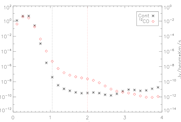
Figure 4: Cut along the blue-shifted (i.e., not affected by cloud extinction) semi-major axis of the disk. The points are correlated (i.e., their separation is smaller than the beam size along the disk’s major axis). The vertical black and red dotted lines show the position at which the emission is higher than $3\times$ the rms of the continuum and moment-0 ${}^{12}\mathrm{CO}$ images, respectively. The negative values are likely artifacts from the cleaning algorithm.

4.5 Inner disk

The shape of the continuum cleaned image is indicative of the presence of an inner cavity. To explore the partially resolved inner disk we here focus on the radially averaged deprojected ALMA visibilities. We split the continuum and ${}^{12}\mathrm{CO}$ visibilities into 30 radial bins, ensuring that all bins contain the same amount of visibilities. This results in minimum and maximum bin sizes of 3.7 k$\lambda$ and 22 k$\lambda$, respectively, and represents a good compromise between $uv$ sampling and error bars. The real part of the binned visibilities of our band-6 observations as a function of $uv$ distance are shown in Fig. 5. The steeper slope of the ${}^{12}\mathrm{CO}$ visibilities shows that the detected gaseous disk is indeed more extended than the dusty disk, as already noticed from the cleaned images. The null in the continuum visibilities at $\sim 150\rm{k}\lambda$ indicates a discontinuity caused by the lack of mm-sized particles in the inner disk regions, or, in other words, the presence of a cavity (see Hughes et al., 2007; Andrews et al., 2011; Hughes et al., 2009). With our observations we cannot estimate the sharpness of the inner wall (see e.g., Mulders, 2013). In the next section we derive the cavity size in the continuum by fitting the $uv$ plane.

The ${}^{12}\mathrm{CO}$ visibilities have lower S/N than the continuum and they are severely affected by the cloud. This complicates the description of the gaseous disk in terms of the analysis of the visibility profile. However, if the gaseous disk velocities are governed by Keplerian rotation, we can use the ${}^{12}\mathrm{CO}$ line profile to estimate how close to the central star we detect gas using the projected observed velocity $v(r)_{Kep}=\sqrt{GM_{\star}/r}\sin{i}$. Assuming that the line center is at $v_{\mathrm{LSR}}=3.4$ km/s, we detect ${}^{12}\mathrm{CO}$ emission down to $v_{\mathrm{LSR}}=0.5$ km/s with a S/N of $\sim$6 (Fig. 2). This corresponds to $-2.9$ km/s in the star’s reference system. Using this velocity, the stellar mass and inclination previously derived, and a distance of $200$ pc, we conclude that our observations probe the ${}^{12}\mathrm{CO}$ gas down to $\sim 28$ au from the central star.

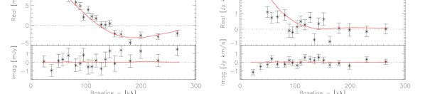
Figure 5: Deprojected, radially binned real and imaginary visibilities as a function of $uv$ distance for the continuum (left) and the gas (right). For the continuum, each bin shows the sum of the visibilities averaged over the continuum channels. For the ${}^{12}\mathrm{CO}$ , each bin shows the sum of the visibilities over the channels containing significant emission (see text). The null in the continuum visibilities at $\sim 125\mathrm{k}\lambda$ indicates the presence of a large inner cavity in the mm-sized dust distribution. The red solid lines show the model discussed in Sect. 5.

5 Radiative transfer model

Based on the obtained observational constraints, in what follows we develop an axisymmetric model for the disk around Sz 91 using the radiative transfer code MCFOST (Pinte et al., 2006, 2009). MCFOST computes the dust temperature structure under the assumption of radiative equilibrium between the dust and the local radiation field. Provided the proper set of parameters, MCFOST creates synthetic SEDs as well as continuum and ${}^{12}\mathrm{CO}$ images. From these images we create synthetic interferometric observations with the same $uv$ coverage as our observations, which are compared with our observations.

We start with a description of our model assumptions about the dust structure, composition, and distribution. Then we use a genetic algorithm (Charbonneau, 1995) to identify a best-fit model that can reproduce our observations.

5.1 Dusty Disk Structure

To account for the SED shape at mid-infrared wavelengths we define two inner disk-regions: the innermost region extending from the dust sublimation radius to $R_{out,1}$ which is severely dust-depleted (“Region 1”) and accounts for the fluxes at 12$\micron$ and below, and the intermediate region extending from $R_{in,2}$ to $R_{out,2}$ (“Region 2”) where some dust is emitting at 22 and 24 µm. There is no observational constrain on the surface density distribution of these two regions, and therefore we adopt a simple power-law of the form

$$\Sigma(r)=\Sigma_{100}\left(\frac{r}{100\mathrm{au}}\right)^{-p_{s}}$$ (1)

where $\Sigma_{100}$ is the surface density distribution at 100 au and $p_{s}$ is the power-law index. We define the outer disk, “Region 3”, as the part of the disk extending from the cavity radius ($R_{\rm{cav}}$) outwards. For a number of disks where the gaseous disk is detected beyond the dusty disk as in Sz 91 a tapered-edge profile can naturally explain the observations (e.g., Hughes et al., 2008; Williams & Cieza, 2011; Andrews et al., 2011; Mathews et al., 2012; Cieza et al., 2012; Zhang et al., 2014). There are three exceptions to this behavior. To explain the high resolution observations of IM Lup, TW Hya and V4046 Sgr strong variations of the gas to dust ratio at large radii are required (Panić et al., 2009; Andrews et al., 2012; Rosenfeld et al., 2013). Our data do not have the high spatial resolution and sensitivity needed to test for radial changes in the gas to dust ratio and therefore we adopt the tapered-edge prescription to describe the outer disk. The surface density distribution in Region 3 is then defined as

$$\Sigma(r)=\Sigma_{C}\,r^{-\gamma}\,\mathrm{exp}\left[-\left(\frac{r}{R_{\rm{C}}}\right)^{2-\gamma}\right],$$ (2)

where $R_{C}$ is the characteristic radius which defines where the tapered-edge begins to dominate over the power-law component, $\Sigma_{C}$ is the surface density at $R_{C}$, and $\gamma$ corresponds to the viscosity power-law index in accretion disk theory ($\nu\propto R^{\gamma}$, Lynden-Bell & Pringle, 1976; Hartmann et al., 1998). For each region we define the scale height $H(r)$ assuming that the dust follows a Gaussian vertical density profile

$$H(r)=H_{0}(r/100\mathrm{au})^{\psi},$$ (3)

where $\psi$ is the flaring parameter of the disk and $H_{0}$ is the scale height at $r=100$ au.

5.2 Dust composition and distribution

We assume homogeneous spherical dust particles. The scattering opacities and phase functions, extinctions and Mueller matrices are computed using Mie theory. For the composition we assumed compact astro-silicates (Mathis & Whiffen, 1989) with a power-law size distribution ($dn(a)\propto a^{-p}da$, with $p=3.5$ e.g., Draine, 2006). This assumption requires minimum and maximum grain sizes of $a_{\mathrm{min}}=2\micron,a_{\mathrm{max}}=15\micron$ in region 1 to not overproduce the flux at 8 and 12 $\micron$ due to the silicate resonance bands. We note that using a different grain composition as e.g. carbon grains it is also possible to match the SED using smaller values of $a_{\mathrm{min}}$ inside the cavity. In any case, the lack of emission above photospheric levels below $8\micron$ indicates that the innermost region of the cavity must be severely depleted of dust particles. Region 2 is mainly constrained by the fluxes at 22, 24 and 70 $\micron$ and therefore many combinations of $a_{\mathrm{min}},a_{\mathrm{max}}$, and the dust mass can reproduce the observed fluxes. The minimum grain size, however, cannot exceed $a_{\mathrm{min}}=0.1\micron$ in order to match the observed fluxes.

5.3 Fitting procedure

We use the stellar parameters derived in Sect. 4.1 and the inclination ($i$) and position angle (PA) derived in Sect. 4.3. We focus on identifying a model that can describe the thermal structure of the disk (constrained by SED and continuum observations) using the disk structure and dust parameters described in the previous sections. Regions 1 and 2 are poorly constrained and therefore we fix the power-law indexes of their surface density distribution to the standard value of $p_{s}=1$ following Andrews & Williams (2007). In Region 1 we fix the minimum and maximum grain sizes to the values discussed in the previous section. Using this prescription we find that we need a maximum dust mass of $M_{dust,1}=1\times 10^{-4}\,M_{\mathrm{\earth}}$ to reproduce the SED shape below 12$\micron$. We adopt this value to describe the dust content inside Region 1. A first exploration of the $H_{0}$ parameter in this region reveals that it is completely unconstrained, and we adopt an arbitrary value of $H_{0_{1}}=5$au. In Regions 1 and 2 we fix the minimum grain size to $a_{min}=0.05\micron$, as in the interstellar medium. For Region 3 we explore the effects of varying the surface density parameter $\gamma$ within the range of $[-1,1]$. We find that our data is equally well fitted with values ranging from $\gamma=[-0.2,0.8]$ and use $\gamma=0.3$. Similarly, our data does not provide observational constraints on the flaring index ($\psi$) in any of the three regions. For all three regions we adopt a typical value of $\psi=1.15$ from model results in , e.g. T Cha (Cieza et al., 2011), IM Lup (Pinte et al., 2008) and HD 163296 (de Gregorio-Monsalvo et al., 2013). Free parameters in our model approach are the outer radius of Region 1 and 2 ($R_{out_{1,2}}$), the inner radius of Region 2 ($R_{in,2}$), and the cavity and characteristic radius of Region 3 ($R_{cav},R_{C}$). We also fit the dust masses $M_{dust_{2,3}}$, the maximum grain sizes $a_{max_{2,3}}$ and the scale heights $H_{0_{2,3}}$.

We explore the parameter space by means of a genetic algorithm. The procedure starts by randomly selecting a number of models. The parameters of these models are defined as their “genes”. Models producing a better match to our observational dataset have the highest chance to reproduce their parameter values (genes) into the next generation of models. The quality of a fit is measured with the combined reduced $\chi^{2}$ given by the sum of reduced $\chi^{2}$ from SED and the continuum visibilities, i.e $\chi^{2}=\chi_{SED}^{2}+\chi_{uv}^{2}$. We use a population of 50 “parent” models and let them evolve through 50 generations, resulting in a total of 2500 models. We find that after 35 generations the models quickly converge, and after 45 generations the variations of each free parameter are within the 5% of the average value of the parameter.

5.4 Modeling results

We find a best-fit model that agrees well with our ALMA observations and with the SED of Sz 91. Its parameters are summarized in Table 3.

Table 3: Model Results. Fixed parameters are listed above the line.

Parameter	Value
$T_{\star}$	$3720$ K
$R_{\star}$	$1.46$ $R_{\sun}$
$M_{\star}$	$0.47$ $M_{\sun}$
$d$	200 pc
$i$	$49.5\arcdeg$
$PA$	$18.2\arcdeg$
$p$	$3.5$
$a_{\rm{min_{1}}},a_{\rm{max_{1}}}$	$2,15$µm
$a_{\rm{min}_{2,3}}$	$0.05\micron$
$H_{0_{1}}$	$5$ au
$p_{s_{1,2}}$	$1$
$\gamma$	$0.3$
$\psi_{1,2,3}$	$1.15$
$M_{\mathrm{dust_{1}}}$	$1\times 10^{-4}$ $M_{\mathrm{\earth}}$
$R_{\rm{1}}$	$0.025$ au
$a_{\rm{max_{2}}}$	$5\micron$
$a_{\rm{max_{3}}}$	$1000$µm
$R_{out_{1}}$	$85$ au
$R_{in_{2}}$	$85$ au
$R_{out_{2}}$	$97$ au
$R_{cav}$	$97$ au
$R_{C}$	$100$ au
$M_{\mathrm{dust_{2}}}$	$0.7$ $M_{\mathrm{\earth}}$
$M_{\mathrm{dust_{3}}}$	$14.3$ $M_{\mathrm{\earth}}$
$H_{0_{2}}$	$5$ au
$H_{0_{3}}$	$10$ au
$\mathrm{log}(\Sigma_{100_{1}})$	$-8.20$ [$gr/cm^{2}$]
$\mathrm{log}(\Sigma_{100_{2}})$	$-2.95$ [$gr/cm^{2}$]
$\mathrm{log}(\Sigma_{C})$	$-1.98$ [$gr/cm^{2}$]

The most significant result of our modeling is that a large cavity of $\sim 97$ au in the dust grain distribution is required to mach our observations. This is clearly illustrated by the null in the real part of the continuum deprojected visibilities as shown in Fig. 5 (left panel). For direct comparison with our ALMA band-6 images we created synthetic ALMA observations using the simalma/casa package. We created an antenna configuration file that mimics our observations using the buildConfigurationFile/Analysis Utilities task. We then run the simulation using the same PWV, exposure time and hour angle as in our observations. The synthetic ALMA image of our model for Sz 91 and the residuals obtained by subtracting the synthetic image from the real observations are shown in Fig. 6 (central and right panels). The residual image has an rms of 0.1 mJy/beam similar to the rms of the observations. Interestingly, our simulated image also shows a brightness difference between the northern and southern lobes of the disk, with the northern lobe being the brighter one (although our MCFOST model image is axisymmetric). To investigate this feature we repeated the SIMALMA/CASA simulations using different $uv$ coverages and PWV. We find that the asymmetry is a consequence of the low S/N of the visibilities at longer baselines as increasing the $uv$ coverage at larger baselines or decreasing the PWV of the simulated ALMA observations removes the apparent difference in brightness.

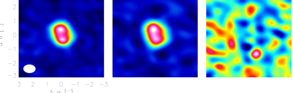
Figure 6: Left: Band-6 continuum observations. Center: Synthetic, ALMA simulated images. Right: Residual image. Notice the different color scale used in this figure.

The SED and surface density distribution of the model are shown in Figs. 7 and 8, respectively. In Fig. 7 we additionally show the individual contributions of Region 1 and Region 2.

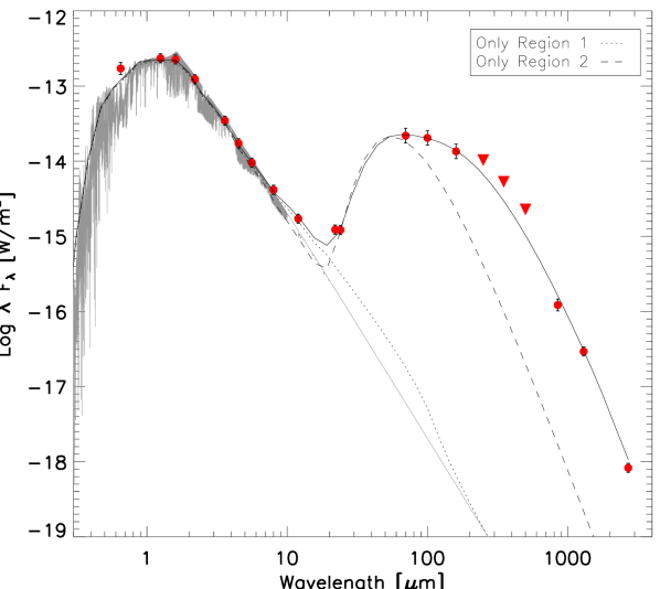
Figure 7: Observed SED of Sz 91, in red symbols. The simulated star’s photosphere is shown in grey. The model described in Sect. 5 is shown as a solid black line. The dotted and dashed lines represent the separate contributions of Region 1 and 2 of our model disk, respectively.

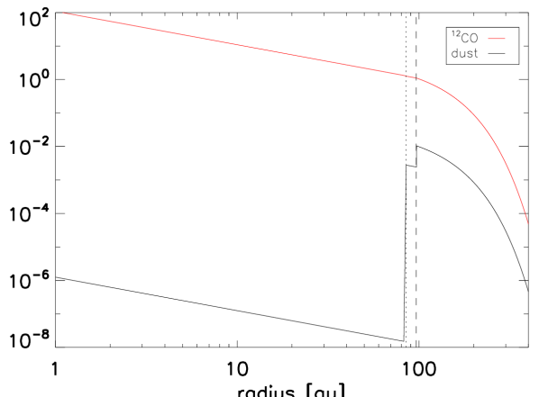
Figure 8: Surface density distribution of the model. The dotted and dashed lines represent $R_{in,2}$ and $R_{cav}$, respectively. The model extends down to 0.025 au (sublimation radius).

5.5 Model uncertainties

To estimate which model parameters are well constrained from our observational dataset we proceed as follow. We fix all but one parameter and run a grid of models exploring the local parameter space. We then derive the reduced $\chi^{2}$ of the models forming this local grid. This procedure is repeated for all free parameters. Keeping in mind that this is equivalent to assume that all parameters are uncorrelated (which is clearly not the case), this approach allow us to get a first idea of which parameters are clearly constrained by our observations without spending unreasonable amounts of computing time. The results of this exploration are shown in Fig. 9. These plots illustrate the severe degeneracy of most of the parameters describing Regions 1 and 2 in our model disk. In contrast, we find that the parameters such as $M_{dust}$, $a_{max}$ and the cavity size ($R_{cav}$) in Region 3 are more constrained by our observations. In particular, values of $R_{cav}$ below 90 au are very difficult to reconcile with the ALMA observations. According to our model, most of the disk’s mass (10 $M_{\earth},\sim 70\%$ of $M_{dust,3}$) is concentrated in a ring ranging from 97 to 140 au.

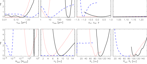
Figure 9: $\Delta\chi^{2}$ (i.e., the difference between the reduced $\chi^{2}$ and its minimum) of the fixed parameters in our modeling (see text). Blue dashed line corresponds to Region 1, red-dotted and black-solid lines indicate Regions 2 and 3, respectively.

5.6 Gaseous Disk

Our observations trace the optically thick ${}^{12}\mathrm{CO}$ line which is severely affected by the cloud. We therefore only present a simple model of the gas component of the disk around Sz 91 that is able to match the ${}^{12}\mathrm{CO}$ line profile reasonably well using standard assumptions. We only consider the blue-shifted (less absorbed) side of the line. Given the sparse observational constrains on the gaseous disk, we build this model upon the best-fit model for the dusty disk obtained in the previous section. The lack of measurements of the isotopologues ${}^{13}\mathrm{CO}$ and $\mathrm{C^{18}O}$ prevents us from estimating the gas to dust ratio and total gas mass as in Williams & Best (2014). We fix the gas to dust ratio in the outer region (Region 3) to the standard value of 100, and we ensure that the ${}^{12}\mathrm{CO}$ freezes-out at 20 K (Qi et al., 2004; de Gregorio-Monsalvo et al., 2013). We assume that the gas and the dust have the same temperature (local thermal equilibrium, LTE). For the ${}^{12}\mathrm{CO}$ abundance we use the standard $\mathrm{H}_{2}$ / ${}^{12}\mathrm{CO}$ ratio ($10^{4}$), which is a reasonable value for protoplanetary disks as confirmed by France et al. (2014). The gas is assumed to be in Keplerian rotation with an inner radius of at least 28 au (in agreement with our observations). Assuming that the gas is in hydrostatic equilibrium in this direction, the gas profile is described by

$$\rho(r,z)=\rho(r,0)\mathrm{exp}\left[-\frac{z^{2}}{2{H(r)}^{2}}\right].$$ (4)

The scale height of the gas component $H(r)$ is given by

$$H(r)=\sqrt{\frac{r^{3}k_{\mathrm{B}}T(r)}{GM_{\star}\mu m_{H}}},$$ (5)

where $k_{\mathrm{B}}$ is the Boltzmann constant, $G$ is the gravitational constant and $m_{H}$ is the Hydrogen mass. We also take into account the thermal broadening of the velocities (defined as $V_{th}=\sqrt{2k_{\mathrm{b}}T_{\mathrm{CO}}/m_{\mathrm{CO}}}$, where $m_{\mathrm{CO}}$ is the molecular mass of the ${}^{12}\mathrm{CO}$ ) and the effect of turbulence ($v_{\mathrm{turb}}$) on the ${}^{12}\mathrm{CO}$ emission along the line of sight.

Under these assumptions, we manually explore different models by varying the turbulence velocity ($v_{\mathrm{turb}}$) within a range of [10,300] m/s (in accordance with the observations discussed by Hughes et al., 2011) and the gas mass inside the dust depleted regions (Region 1 and 2). We find a model that agrees relatively well with our observations using a continuous gaseous disk (i.e. without depletion or inner cavity) with $v_{\mathrm{turb}}=120$ m/s. The radially binned deprojected visibilities and the surface density of this model are shown in Fig. 5 (right panel) and Fig. 8 (red line), respectively. The integrated ${}^{12}\mathrm{CO}$ line profile of the model, along with the real observations, is shown in Fig. 10.

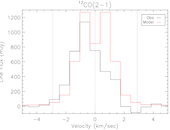
Figure 10: Observed ${}^{12}\mathrm{CO}$ line profile, in black histogram. The velocity scale is centered at the reference system of the star, using $v_{\mathrm{LSR}}=3.4$ km/s. The profile was computed by integrating the flux contained in the $>3\sigma$ region of the moment-0 image (white dashed contour in central panel of Fig. 2) in each channel. The vertical dotted lines show the center of the line and the highest velocity bin observed at $>3\sigma$ significance, corresponding to -2.9 km/s. The vertical dotted line at 2.9 km/s highlights the strong absorption-like effect on the red-shifted side of the ${}^{12}\mathrm{CO}$ line. The red histogram shows the gas model presented in Sect. 5.

6 Discussion

6.1 Are three zones required?

Assuming three different disk regions we find a model that reproduces reasonably well our observational dataset. As a separate exercise we also tried to fit a disk model composed by only two regions (the inner cavity and the outer disk). After running the genetic search we could not find a good match to our observations with such a disk structure. This result is in agreement with the findings of T2014, who need an extra component, either a circumplanetary disk or a narrow, optically thick inner ring, to reproduce the fluxes at 22 and 24$\micron.$

6.2 Model limitations

The local parameter exploration (Fig. 9) represents a useful approach to estimate how sensitive are the model parameters to our observations. We find that most of the parameters describing Region 1 and 2 remain unconstrained from our observations. For instance, in our representative model there are no empty gaps as we find $R_{out,1}=R_{in,2}$ and $R_{out,2}=R_{cav}$, although other values for these parameters (i.e., an empty gap between Region 1 and 2, or a dust empty innermost region) could equally reproduce our observations (as indicated by the $\Delta\chi^{2}$ profile in the $R_{in}$ and $R_{out}$ panels in Fig.9). For all 3 regions we find that the the exponents of the surface density distributions are completely unconstrained by our observations. The same happens with the flaring index $\psi$, as expected if the emission is optically thin at these wavelengths. However, the exercise we performed does not allow to derive proper statistical errors of the fitted parameters as we did not investigate correlations between the parameters. The latter would require to map the entire multidimensional parameter space which is beyond the scope of this paper and which would require to spend an unreasonable amount of computing time. We reserve this exercise for the future, when data with more sensitivity and much better angular resolution will be available. Regarding the gas model, we find that it is difficult to reproduce the observed ${}^{12}\mathrm{CO}$ profile with our model. Overall we see that compared to the observations the model shows a lack of emission at higher velocities, and an excess at lower velocities. Even using a non-depleted gaseous disk our model produces less flux at higher velocities than the observations. We note that this does not exclude the possibility of a gas-depleted cavity (as found for HD 142527, Perez et al., 2014), since we also find that it is possible to produce a similar ${}^{12}\mathrm{CO}$ profile modeling a gas-depleted cavity using higher values of turbulence, or using different surface density profiles for the gaseous and dusty disks (i.e., different $\gamma$ for the gas and dust disks).

6.3 Cavity-making mechanism

With a size of 97 au in radius, Sz 91 has by far the largest the inner cavity observed in a transition disk around a T Tauri star. This cavity size and accretion rate ($7.9\times 10^{-11}\mathrm{M_{\sun}}\,\mathrm{yr}^{-1}$) exclude photoevaporation alone as the mechanism responsible for the cavity (e.g., Rosotti et al., 2013; Owen et al., 2012). Similarly, studies of grain growth conclude that grain growth alone cannot produce the large cavities resolved by interferometric mm observations (Birnstiel et al., 2013). Romero et al. (2012) excluded a stellar companion down to separations of $\sim 30$ au with a contrast of $\Delta K\sim 3.3$. Using NextGen models (e.g. Allard et al., 1997), an age of 1 Myr and the stellar mass derived in Sect. 4.1 translates into a sensitivity close to the brown dwarf limit of $\sim 80~{}\mathrm{M_{J}}$. In addition, Melo (2003) found no evidence for a close-in binary companion around Sz 91 in their 3-years radial velocity survey (down to masses of $\approx 0.2\mathrm{M}_{\odot}$). However, we cannot yet exclude that a low mass stellar companion is carving the cavity in the disk around Sz 91. The other possible mechanism is planet formation. In fact, our direct detection of gas inside of the large dust-depleted cavity, the presence of $\micron$-sized dust inside the cavity, and the large cavity size indicated by the continuum visibilities matches well several predictions of models for multiple (Jupiter-sized) planet formation (e.g. Lubow & D’Angelo, 2006; Dodson-Robinson & Salyk, 2011; Zhu et al., 2011).

6.4 Inner disk structure: planet formation signature?

There are at least four transition objects with detectable (but different) accretion rates that can be explained by an inner disk structure similar to the one derived for Sz 91. DM Tau and RX J1615.3-3255 have resolved cavities and require an empty disk very close to the star because of the lack of NIR excess, but some dust in the outer regions of the cavity to account for the MIR emission (Andrews et al., 2011). However, a direct comparison with Sz 91 is difficult because the modeling approach adopted by Andrews et al. (2011) is different from ours. RX J1633.9-2442 and [PZ99] J160421.7-213028 have been analyzed using similar tools than those used in this work for Sz 91. In both systems, an empty inner disk and some dust inside the main cavity (Cieza et al., 2012; Mathews et al., 2012; Zhang et al., 2014) are needed to explain the mm-observations and SED. Interestingly, the mm-sized dust distribution in [PZ99] J160421.7-213028 is concentrated in a ring similar to what we find for Sz 91 (Zhang et al., 2014; Mathews et al., 2012). Pinilla et al. (2012) concludes that this ring-shaped dusty structure is a product of the planet-disk interaction.

While in all five cases strong parameter degeneracies of the models do not allow us to constrain the exact configuration of the dust inside the cavity, photoevaporation and grain growth can be ruled out as the mechanisms carving the inner hole of these disks. Furthermore, for DM Tau, RX J1633.9-2442, and [PZ99] close binarity can also be excluded and planet-formation has been suggested to explain both the cavities and the presence of dust inside the cavity (e.g., Rice et al., 2006; Cieza et al., 2012; Mathews et al., 2012). As suggested by Cieza et al. (2012), these inner structures are likely simple approximations to the complex structures predicted by hydrodynamical models of planet formation (Dodson-Robinson & Salyk, 2011), which have now been directly observed (e.g., Casassus et al., 2013; Quanz et al., 2013) in a few systems.

7 Conclusions

We presented ALMA band-6 and band-3 observations of Sz 91 which clearly show that there must be a very large inner cavity in the disk around Sz 91. We also detect ${}^{12}\mathrm{CO}$ gas inside the cavity down to at least 28 au. We detect gas at larger radii (400 au) than the dust (220 au). We used a genetic algorithm to construct an MCFOST model of the disk around Sz 91 explaining our ALMA observations and the SED of the system. We find that a three-zone model is required to fully explain the observations. The inner region of the disk is significantly depleted of dust particles, and there are $\approx 0.7\rm{M}_{\earth}$ of dust confined within the 85-97 au region. The exact spatial distribution of the dust in these two regions is not constrained by the available observations but our $uv$-fit to the data indicates that the dust depleted region extends to $\sim 97$ au. This implies that there must be significant amounts of gas inside the dust depleted inner regions. The bulk of the dust mass is located in a ring extending from 97 au to 140 au. The different outer radius observed for the ${}^{12}\mathrm{CO}$ and the dust can be explained by an exponential tapered surface density profile.

A yet undetected, very low mass companion (below $0.2\mathrm{M_{\sun}}$) in the inner 30 au, could create the large cavity observed in Sz 91. However, the size of the disk’s cavity and the presence of gas and small dust particles inside the cavity agree remarkable well with the theoretical predictions for multiple, Jupiter-sized, planet formation. Considering its spectral type and low stellar mass, Sz 91 has an extremely large inner cavity when compared with other transition disks (e.g. Andrews & Williams, 2007). Finally, we find that similar structures of the inner regions of dusty disks are also observed in at least four other planet-forming candidates transition disks. It is tempting to interpret the inner disk structure and large cavity size as a signpost of forming planets inside these disks.

References

- Alexander et al. (2006) Alexander, R. D., Clarke, C. J. & Pringle, J. E. 2006, MNRAS, 369, 229
- Allard et al. (1997) Allard, F., Hauschildt, P. H., Alexander, D. R. & Starrfield, S., 1997, ARA&A, 35
- Andrews & Williams (2007) Andrews, S. M. & Williams, J. P., 2007, ApJ, 659, 705
- Andrews et al. (2011) Andrews, S. M., Wilner, D. J., Espaillat, C. et al. 2011, ApJ, 732, 42
- Andrews et al. (2012) Andrews, S. M., Wilner, D. J., Hughes, A. M. et al. 2012, ApJ, 744, 162
- Artymowicz & Lubow (1994) Artymowicz, P. & Lubow, S. H. 1994, ApJ, 421, 651
- Birnstiel et al. (2013) Birnstiel, T., Andrews, S. M. & Ercolano, B. 2013, A&A, 544, A79
- Birnstiel et al. (2013) Birnstiel, T. & Andrews, S. M. 2013, ApJ, 780,153
- Bustamante et al. (2015) Bustamante, I., Merín, B., Ribas, Á. et al. 2015, A&A, in press
- Casassus et al. (2013) Casassus, S., van der Plas, G., Perez, S. M. et al. 2013, Nature, 493, 191
- Charbonneau (1995) Charbonneau, P. 1995, ApJS, 101, 309
- Cieza et al. (2007) Cieza, L. A., Padgett, D. L. , Stapelfeldt, K. R. et al. 2007, ApJ, 667, 308
- Cieza et al. (2011) Cieza, L. A., Olofsson, J., Harvey, P. M. et al. 2011, ApJ, 741, L25
- Cieza et al. (2012) Cieza, L. A., Mathews, G. S. Williams et al. 2012, ApJ, 752, 75
- Cutri et al. (2003) Cutri, R. M. , Skrutskie, M. F., van Dyk, S., et al. 2003, The 2MASS All-Sky Catalog of Point Sources (Pasadena, CA: University of Massachusetts and Infrared Processing and Analysis Center, IPAC/California Institute of Technology)
- Dodson-Robinson & Salyk (2011) Dodson-Robinson, S. E. & Salyk, C. 2011, ApJ, 738, 131
- Draine (2006) Draine, B. T, 2006, ApJ, 636, 1114
- Dullemond & Dominik (2005) Dullemond, C. P. & Dominik, C. 2005, A&A, 434, 971
- Evans et al. (2009) Evans, N., Calvet, N., Cieza, L., et al. 2009, arXiv:0901.1691
- France et al. (2014) France, K., Herczeg, G. J., McJunkin, M. & Penton, S. V. 2014, ApJ, 794, 60
- de Gregorio-Monsalvo et al. (2013) de Gregorio-Monsalvo, I., Ménard, F., Dent, W. et al. 2013, A&A, 557, A133
- Hartmann et al. (1998) Hartmann, L., Calvet, N., Gullbring, E. & D’Alessio, P. 1998, ApJ, 495,385
- Högbom, J. A. (1974) Högbom, J. A.. 1974, A&AS, 15, 417
- Hughes et al. (1994) Hughes, J., Hartigan, P., Krautter, J. & Kelemen, J. 1994, AJ, 108, 1071
- Hughes et al. (2007) Hughes, A. M., Wilner, D. J., Calvet, N. et al. 2007, ApJ, 664, 536
- Hughes et al. (2008) Hughes, A. M., Wilner, D. J., Qi, C. & Hogerheijde, M. R. 2008, ApJ, 678,1119
- Hughes et al. (2009) Hughes, A. M. , Andrews, S. M., Espaillat, C. et al. 2009, ApJ, 698, 131
- Hughes et al. (2011) Hughes, A. M. , Wilner, D. J., Andrews, S. M., Qi, C. & Hogerheijde, M. R., 2011, ApJ, 727, 85
- Lin & Papaloizou (1986) Lin, D. N. C. & Papaloizou, J. 1986, ApJ, 309, 846
- Lynden-Bell & Pringle (1976) Lynden-Bell, D. & Pringle, J. E. 1974, MNRAS, 168, 603
- Lubow & D’Angelo (2006) Lubow, S. H. & D’Angelo, G. 2006, ApJ, 641, 526
- Mathews et al. (2012) Mathews, G. S., Williams, J. P. & Ménard, F. 2012, ApJ, 753, 59
- Mathis & Whiffen (1989) Mathis, J. S. & Whiffen, G., 1989, ApJ, 341, 808
- McMullin et al. (2007) McMullin, J. P. , Waters, B. , Schiebel, D., Young, W. & Golap, K. 2007, Astronomical Data Analysis Software and Systems XVI, 376, 127
- Melo (2003) Melo, C. H. F. 2003, A&A, 410, 269
- Merín et al. (2008) Merín, B., Jorgensen, J., Spezzi, L. et al. 2008, ApJS, 177, 551
- Mulders (2013) Mulders, G. D., Paardekooper, S.-J., Panić, et al. 2013, A&A, 557, 68
- Owen et al. (2012) Owen, J., Clarke, C. J. & Ercolano, B. 2012, MNRAS, 422, 1880
- Panić et al. (2009) Panić, O., Hogerheijde, M. R., Wilner, D. & Qi, C., 2009, A&A, 501, 260
- Perez et al. (2014) Perez, S., Casassus, S., Ménard, F., et al. 2015, ApJ, 798, 95
- Pinilla et al. (2012) Pinilla, P., Benisty, M., & Birnstiel, T. 2012, A&A, 545, A81
- Pinilla et al. (2014) Pinilla, P., Benisty, M., Birnstiel, T., Ricci, L. et al. 2014, A&A, 564, A51
- Pinte et al. (2006) Pinte, C., Ménard, F., Duchene, G. & Bastien, P. 2006, A&A, 459, 797
- Pinte et al. (2008) Pinte, C., Padgett, D. L., Ménard, F. et al. 2008, A&A, 489, 633
- Pinte et al. (2009) Pinte, C., Harries, T. J., Min, M., et al. 2009, A&A, 498, 967
- Qi et al. (2004) Qi, C., Ho, P. T. P., Wilner, D. J., Takakuwa, S. et al. 2004, ApJ, 616, L11
- Quanz et al. (2013) Quanz, S. P. , Avenhaus, H., Buenzli, E., Garufi, A. et al. 2013, ApJ, 2013, 766
- Rice et al. (2006) Rice, W. K. M., Armitage, P. J., Wood, K. & Lodato, G. 2006, MNRAS, 373, 1619
- Ricci et al. (2012) Ricci, L., Trotta, F.. Testi, L. et al. 2012, A&A, 540, A6
- Romero et al. (2012) Romero, G. A., Schreiber, M. R., Cieza, L. A et al. 2012, ApJ, 749, 79
- Rosotti et al. (2013) Rosotti, P. G., Ercolano, B., Owen, J. & Armitage, P. J. 2013, MNRAS, 430, 1392
- Rosenfeld et al. (2013) Rosenfeld, K. A, Andrews, S. M., Wilner, D. J., Kastner, J. H. & McClure, M. K. 2013, ApJ, 775, 136
- Siess et al. (2000) Siess, L., Dufour, E. & Forestini, M. 2000, A&A, 358, 593
- Tachihara et al. (2001) Tachihara, K., Toyoda, S., Onishi, T. et al. 2001, PASJ, 53,1081
- Tsukagoshi et al. (2014) Tsukagoshi, T., Momose, M., Hashimoto, J. et al. 2013, ApJ, 783, 90
- Vilas-Boas et al. (2000) Vilas-Boas, J. W. S., Myers, P. C. & Fuller, G. A. 2000, ApJ, 532, 1038
- Williams & Cieza (2011) Williams, J. P. & Cieza, L. A. 2011, ARA&A, 49, 67
- Williams & Best (2014) Williams, J. P. & Best, W. M. J., 2014, ApJ, 788, 59
- Wright et al. (2010) Wright, E., L.; Eisenhardt, P., R., M., Mainzer, A. K. et al. 2010, AJ, 140, 1868
- Zacharias et al. (2010) Zacharias, N., Finch, C., Girard, T. et al. 2010, AJ, 139, 2184
- Zhang et al. (2014) Zhang, K., Isella, A., Carpenter, J. M. & Blake, G., A 2014, ApJ, in press
- Zhu et al. (2011) Zhu, Z., Nelson, R. P. , Hartmann, L., Espaillat, C. & Calvet, N. 2011, ApJ, 729, 47