Baryon and chiral symmetry breaking in holographic QCD

Abstract

We study the relationship between chiral symmetry breaking and baryons in holographic QCD. We construct a soliton with unit baryon charge in the presence of a nonzero mean value of the scalar bifundamental field, which is dual to the chiral condensate. We obtain a relation between the chiral condensate and the mass of the baryon and find in a clear-cut way that at large values of the condensate the holographic soliton is no longer located on the IR wall. Instead it is split into two halves, which are symmetrically located on the left and right flavor branes. On the other hand we find that the local value of the quark condensate is suppressed in the core of the soliton, which is evidence for a partial chiral symmetry restoration inside the baryon.

I Introduction

Baryon physics in holographic setups has been addressed since the time the first holographic QCD models have been developed. There is a wealth of works related to the interpretation of the baryon as a holographic instanton Hata:2007mb ; Bolognesi:2013nja ; Rozali:2013fna , the QCD currents sourced by the baryon Hashimoto:2008zw ; Hong:2007dq ; Kim:2008pw and even high-density baryonic matter Kaplunovsky:2012gb ; Dymarsky:2010ci ; Rho:2009ym . Unfortunately though, the studies of the interplay between baryon physics and physics of chiral symmetry breaking is undeservedly rare: Ref.Domenech:2010aq is the only example that we are aware of. But from the other hand these relationships remain one of the longstanding questions in QCD ioffe and should be definitely addressed with the new tools provided by the holographic duality, which proved to be useful in describing both chiral symmetry breaking and baryons in QCD.

Usually the AdS/QCD model, which is used for the studies of baryons, is (a modification of) the Sakai-Sugimoto model (SS) Sakai:2004cn ; Sakai:2005yt . This model is based on the system of $N_{f}$ $D8-\overline{D8}$ branes, which are embedded in the curved hyperbolic space produced by a stack of $N_{c}$ $D4$ branes. One of the dimensions, $\tau$, is compact and serves for breaking supersymmetry. The compactification radius of $\tau$ vanishes at some point and thus the background space has the shape of a cigar Witten:1998zw . The location of the tip of the cigar plays the role of the $\Lambda_{QCD}$ scale. From the holographic point of view, the tip serves as a boundary beyond which nothing can propagate as the space practically ends there. The $D8-\overline{D8}$ branes embedded in this background are located at the opposite (or almost opposite Seki:2008mu ) points of the $\tau$-circle and consequently they merge together when the circle collapses. The gauge field, $\mathcal{A}$, which is a massless mode of the open string with two ends connected to the $D8$ branes, belongs to the adjoint representation of the flavor group $U(N_{f})$ and is dual to the quark current operator of QCD. One can introduce the coordinate $U$ along the branes with the origin on the tip of the cigar, which goes from $-\infty$ on the $D8$ brane to $+\infty$ on the $\overline{D8}$ brane. The values of the gauge field $\mathcal{A}$ at $-\infty$ may be thought of as being coupled to the left quark current $J^{aL}_{\mu}=\bar{q}\frac{1+\gamma_{5}}{2}\gamma_{\mu}t^{a}q$ while the values at $\infty$ are coupled to the right current $J^{aR}_{\mu}=\bar{q}\frac{1-\gamma_{5}}{2}\gamma_{\mu}t^{a}q$. Accordingly one can call the $D8$ branes Left and the $\overline{D8}$ branes Right.

The baryon in the Sakai-Sugimoto model is an instanton of the field $\mathcal{A}$ Hata:2007mb . The baryon charge equals the topological charge of the instanton because the baryon current is sourced in the Chern-Simons (CS) term of the action by a topological charge density. One can find that the instanton in the SS model is well approximated by the usual flat BPST instanton. This holds because the size of the instanton is parametrically small; the center of the solution is located on the tip of the cigar and one can neglect the curvature of the metric at the scale of the solution radius. The vanishing difference between spatial ($x_{i},i=1,\dots,3$) and holographic ($U$) parts of the metric leads to an approximate $SO(4)$ symmetry group of the space Bolognesi:2013nja . In this setting it is very convenient to use the usual radial ansatz of the BPST instanton with the radial coordinate $\rho^{2}=U^{2}+\Sigma x_{i}^{2}$. The solution is then located at $\rho=0$.

For our purposes, though, the Sakai-Sugimoto model is not entirely satisfactory. The obstacle is that it is not at all easy to describe chiral symmetry breaking and the associated chiral condensate in this setup. This problem was analyzed in Refs. Bergman:2007pm ; Dhar:2008um and it was shown that the holographic field dual to the scalar quark current $\bar{q}q$ is a tachyonic mode of the string stretched between the $D8$ and the $\overline{D8}$ branes. The tachyonic field condenses on the tip of the cigar, thus providing a nonzero vacuum expectation value (VEV) of $\bar{q}q$, the chiral condensate. There are, however, several complications in this setup. The construction of the tachyonic DBI action is ambiguous, the backreaction of the condensed open string on the geometry of space should be taken into account and so on. On top of that, when constructing an effective 5-dimensional holographic model for mesons it is impossible to treat the open string as a local field.

The chiral symmetry breaking is relatively easy to implement in the other, “bottom-up”, approach of holographic QCD. Instead of constructing the brane system which would reproduce the effective theory of mesons, one builds the model by including the fields, dual to the QCD operators, in the 5-dimensional AdS background Erlich:2005qh ; Karch:2006pv . In the “hard-wall” (HW) model Erlich:2005qh the space ends on the wall located at a finite value of the holographic coordinate $z_{m}$. This wall (we will call it the IR wall) serves the same purpose as the tip of the cigar in the SS model by breaking conformal symmetry and providing the scale $\Lambda_{QCD}$. There are two gauge fields $\bm{L}$ and $\bm{R}$, which are dual to left and right quark currents. The field, which is dual to the scalar quark operator $\bar{q}q$, is just a bifundamental scalar $\bm{X}$. Its vacuum profile is described by the two parameters

$$\bm{X}_{0}=\frac{\mathbbm{1}}{2}\big{(}mz+\sigma z^{3}\big{)},$$ (1)

which by the holographic dictionary gubser-klebanov are related to the quark mass $m$ and condensate (see Refs. Krikun:2008tf ; Gorsky:2009ma ; Cherman:2008eh and the derivation in Sec. VI)

$$\langle\bar{q}q\rangle=\frac{N_{c}}{2\pi^{2}}\sigma.$$ (2)

In the model there is no internal mechanism, which would fix the value of the chiral condensate. Instead one obtains a nonzero value of $\sigma$ by imposing a Dirichlet boundary condition on $\bm{X}$ at the IR wall

$$\bm{X}\Big{|}_{z=z_{m}}=\frac{\mathbbm{1}}{2}\big{(}mz_{m}+\sigma z_{m}^{3}\big{)}={\rm const}.$$ (3)

One can obtain the correlation functions of various operators in the setup with nonzero profile of the bifundamental scalar and study the dependence of various observables on the chiral condensate, which is just a parameter of the model. Unfortunately, the treatment of the baryon in this setup is not as straightforward as it is in the SS model. There are two gauge fields, which should realize the topologically nontrivial solution, and on top of that, there is a scalar with a nonzero VEV, which interacts with both of them. One should also pay special attention to the boundary conditions at the IR boundary, as they are arbitrary in the construction and should be additionally fixed in the model. Concerning the baryon, the question of IR boundary condition becomes substantially important because the corresponding topological soliton falls on the IR wall, a phenomenon similar to the localization of the SS-instanton on the tip of the cigar. The baryon physics in HW model without a chiral condensate was addressed in Ref. Pomarol:2008aa .

The bifundamental scalar was included in Ref. Domenech:2010aq , however the dependence of the baryon mass on the condensate has not been investigated. Motivated by the formula derived using the QCD sum rules in Ref. ioffe two of us have analyzed the baryon-mass origin in the framework of the hard wall model gk ; gkk and found that at large values of the chiral condensate, there are clear indications that it dominates. However the accuracy of the numerical calculations was not high enough to make precise claims. In this paper we perform a detailed analysis of the different aspects of the impact of the chiral symmetry breaking on the baryon solution. We will clearly see the internal structure of the solution and two regimes in the dependence of the baryon mass on the chiral condensate.

The paper is organized as follows. In Sec. II we introduce our setup, which we try to keep sufficiently general and applicable to a wide range of holographic QCD models. We study the qualitative structure of the baryon solution in the presence of the chiral scalar field in Sec. III. The quantitative support for this treatment is given by the numerical solution in Sec. IV. Secs. V and VI are devoted to the calculation of the baryon mass and local mean values of the QCD currents in presence of the baryon. We conclude in Sec. VII. The analysis of the precision of our numerics is outlined in the Appendix.

II The model

It is actually possible to make a qualitative connection between the seemingly different setups of the Sakai-Sugimoto and the “hard wall” models. In order to build up our intuition we use the following “folding trick”: Consider the cigar-bended $D8$ brane of the SS model. There is a single gauge field $\mathcal{A}$ on this brane, but let us call it $\bm{L}$ when it is considered on the Left brane and $\bm{R}$ on the Right brane (see Fig. 1). On the tip of the cigar $\bm{L}=\bm{R}$, of course. Next, let us assume trivial dynamics along the $\tau$ direction, which will allow us to neglect the separation of the branes along $\tau$ altogether, effectively “folding” the cigar-shaped brane into a single sheet. More specifically, we cut the brane along the tip or $U=0$ line. On one side we have the $\bm{L}$ field and $U\in[0;+\infty)$ and on the other side the $\bm{R}$ field and $U\in(-\infty;0]$. In order to get consistent coordinates, we perform a $U\rightarrow-U$ transformation on the Right brane, which also means $\bm{R}_{U}\rightarrow-\bm{R}_{U}$. It is convenient to introduce the inverse holographic coordinate $z=1/(U+z_{m}^{-1})$. Then the tip of the cigar ($U=0$) corresponds to the maximum $z=z_{m}$ and the boundary values are assigned at $z=0$. At the end of the day we have two gauge fields propagating on a strip $z\in(0,z_{m}]$, which is qualitatively the same as in the HW model. The important additional information, that we get here, is the boundary conditions on the gauge fields at the IR boundary. Because we know that $\bm{L}$ and $\bm{R}$ are the same field there, we get

$$\mathrm{IR:}\qquad\bm{L}_{z}+\bm{R}_{z}=0,\qquad\bm{L}_{\mu}-\bm{R}_{\mu}=0.$$ (4)

In this picture the tachyonic string, which was responsible for the chiral condensate in the SS model, collapses to the local bifundamental tachyonic scalar $\bm{X}$. The SS baryon, which was originally located at $U=0$, is now split into two halves, one composed of $\bm{L}$ and the other of $\bm{R}$, which are folded together. Thus we expect that in the HW model, the baryon would appear as one half of the instanton lying on the IR wall.

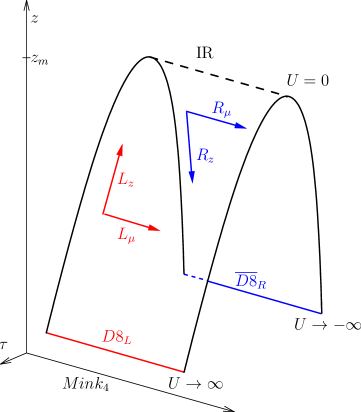
Figure 1: Scheme of the “folding trick” explained in the text.

As we see, in any case the holographic QCD model with two quark flavors $N_{f}=2$ can be described by dynamics of left ($\bm{L}$) and right ($\bm{R}$) gauge fields of the group $U(2)_{L}\times U(2)_{R}$ and a bifundamental tachyonic scalar $\bm{X}$ in 5-dimensional curved space. We use Hermitian gauge-group generators and treat the gauge connection as Hermitian matrices:

$$\bm{L}=\hat{L}\ \frac{\mathbbm{1}}{2}+L=\hat{L}\ \frac{\mathbbm{1}}{2}+L^{a}t^{a},\qquad a=1,\dots,3,$$ (5)

$$t^{a}=\frac{\sigma^{a}}{2},\qquad\mathrm{tr}(t^{a}t^{b})=\frac{1}{2}\delta^{ab},\qquad[t^{a},t^{b}]=i\epsilon^{abc}t^{c}.$$

where $\sigma^{a}$ are the Pauli matrices. The background space can be described by the mostly-minus metric of the general form

$$ds^{2}=h(z)^{2}dt^{2}-h(z)^{2}dx_{i}^{2}-k(z)^{2}dz^{2},\qquad t\equiv x_{0},\ z\equiv x_{5},\ i=1,\dots,3.$$ (6)

For instance, in the “hard-wall” model Erlich:2005qh $k(z)=h(z)=L/z$; in Sakai-Sugimoto model Sakai:2004cn $h(z)=(L/z)^{3/4},\ k(z)=(L/z)^{1/4}(1-\frac{z^{3}}{z_{m}^{3}})^{-1/2}$. $L$ is a curvature scale and the holographic coordinate $z$ is bounded from above: $z\in(0;z_{m}]$. The Yang-Mills action is

$$S_{YM}=\int d^{3}xdtdz\bigg{\{}-\frac{1}{4g_{5}^{2}} \mathrm{Tr}\Big{\langle}k(z){\bm{F}_{L}}_{ij}^{2}-2k(z){\bm{F}_{L}}_{0i}^{2}+2\frac{h(z)^{2}}{k(z)}\left({\bm{F}_{L}}_{5i}^{2}-{\bm{F}_{L}}_{50}^{2}\right)+(\bm{L}\leftrightarrow\bm{R})\Big{\rangle}$$ (7)

$$+g_{X}^{2} \mathrm{Tr}\Big{\langle}h(z)^{2}\left(D_{0}\bm{X}^{2}-D_{i}\bm{X}^{2}\right)-\frac{h(z)^{4}}{k(z)}(D_{5}\bm{X})^{2}-h(z)^{4}k(z)m_{X}^{2}|\bm{X}|^{2}\Big{\rangle}\bigg{\}},$$

where the covariant derivative is $D_{*}\bm{X}=\partial_{*}\bm{X}-i\bm{L}_{*}\bm{X}+i\bm{X}\bm{R}_{*}$ and the gauge coupling $g_{5}$ and normalization of the scalar $g_{X}$ are to be fixed by phenomenology Erlich:2005qh ; Krikun:2008tf ; Gorsky:2009ma ; Cherman:2008eh or a specific top-down construction Sakai:2004cn ; Bergman:2007pm . The mass of the scalar $m_{X}$ is defined by the dimension of the corresponding operator $q^{\alpha}\bar{q}^{\beta}$ and equals $m_{X}^{2}=-\frac{3}{L^{2}}$.

The Chern-Simons term is present as well

$$S_{CS}=\frac{N_{c}}{24\pi^{2}}\int\frac{3}{2}\ \left\{\hat{L}\wedge\mathrm{Tr}\left\langle F_{L}\wedge F_{L}\right\rangle-(\bm{L}\leftrightarrow\bm{R})\right\}+\dots.$$ (8)

One can immediately spot that the non-Abelian part of the gauge field, which has nonzero topological charge in the 4-dimensional spacelike slice, provides a source for the temporal component of the Abelian field, which is dual to the baryon current. Thus we can identify the baryon charge of a given field configuration Hata:2007mb ; Pomarol:2008aa

$$Q_{B}=\frac{1}{16\pi^{2}}\int d^{3}xdz\;\epsilon^{mnlk}\left({F_{L}^{a}}^{mn}{F_{L}^{a}}^{lk}-{F_{R}^{a}}^{mn}{F_{R}^{a}}^{lk}\right),\qquad m=1,\dots,3,5.$$ (9)

In order to construct the solution in the 4D spacelike $(x_{i},z)$-plane we adopt the cylindrical ansatz proposed in Refs. Witten_inst ; Pomarol:2008aa ; Domenech:2010aq , taking $r=\sqrt{x_{i}^{2}}$ and $z$ as the cylindrical coordinates. The 4D gauge potentials are parametrized by all possible tensor structures which link the spatial and $SU(2)$ group indices. It is convenient to work with the vector and axial combinations, defined as

$$\bm{L}=\bm{V}+\bm{A},\qquad\bm{R}=\bm{V}-\bm{A}.$$ (10)

In order to preserve 3D parity, we choose the P-odd and P-even tensors for the spatial components of $V_{i}=(L_{i}+R_{i})/2$ and $A_{i}=(L_{i}-R_{i})/2$, respectively. Similarly, the time and $z$ components should be parity even for $V$ and odd for $A$. Hence we obtain the following ansatz for the gauge fields

$$V_{j}^{a} =-\frac{1+\eta_{2}(r,z)}{r}\epsilon_{jak}\frac{x_{k}}{r}, V_{5}^{a} =0, \hat{V}_{0} =v(r,z),$$ (11)

$$A_{j}^{a} =\frac{\eta_{1}(r,z)}{r}\left(\delta_{ja}-\frac{x_{j}x_{a}}{r^{2}}\right)+A_{r}(r,z)\frac{x_{j}x_{a}}{r^{2}}, A_{5}^{a} =A_{z}(r,z)\frac{x_{a}}{r}, \hat{A}_{0} =0.$$

For the scalar we have

$$X=\chi_{1}(r,z)\frac{\mathbbm{1}}{2}+i\chi_{2}(r,z)\frac{t^{a}x^{a}}{r}.\\$$ (12)

The action (7) with this ansatz is $S=\int dtdrdz\big{(}\mathcal{L}_{YM}+\mathcal{L}_{U1}+\mathcal{L}_{CS}\big{)}$:

$$\mathcal{L}_{YM} =-\frac{2\pi}{g_{5}^{2}}\bigg{\{}r^{2}\frac{h(z)^{2}}{k(z)}\big{[}\partial_{z}A_{r}-\partial_{r}A_{z}\big{]}^{2}$$ (13)

$$\phantom{=-\frac{2\pi}{g_{5}^{2}}\bigg{\{}\ }+\frac{2}{k(z)}\Big{[}k(z)^{2}\mathcal{D}_{r}\eta_{\alpha}^{2}+h(z)^{2}\mathcal{D}_{z}\eta_{\alpha}^{2}\Big{]}\bigg{\}}$$ (14)

$$-2\pi g_{X}^{2}\bigg{\{}r^{2}\frac{h(z)^{2}}{k(z)}\Big{[}k(z)^{2}\mathcal{D}_{r}\chi_{\alpha}^{2}+h(z)^{2}\mathcal{D}_{z}\chi_{\alpha}^{2}+m_{X}^{2}h(z)^{2}k(z)^{2}\chi_{\alpha}^{2}\Big{]}$$ (15)

$$\phantom{=-\frac{2\pi}{g_{5}^{2}}\bigg{\{}\ }+2\ \frac{h(z)^{4}}{k(z)}\big{[}\chi_{2}\eta_{2}+\chi_{1}\eta_{1}\big{]}^{2}+\frac{1}{g_{X}^{2}g_{5}^{2}}\frac{k(z)}{r^{2}}\left(1-\eta_{\alpha}^{2}\right)^{2}\bigg{\}},\quad\alpha=1,2,$$ (16)

$$\mathcal{L}_{U1} =\left(\frac{4\pi}{2g_{5}^{2}}\right)\frac{r^{2}}{k(z)}\Big{[}h(z)^{2}(\partial_{z}v)^{2}+k(z)^{2}(\partial_{r}v)^{2}\Big{]},$$ (17)

$$\mathcal{L}_{CS} =\left(\frac{N_{c}}{2\pi}\right)\ v\ \Big{[}2\epsilon^{\alpha\beta}\mathcal{D}_{z}\eta_{\alpha}\mathcal{D}_{r}\eta_{\beta}+\big{(}\partial_{z}A_{r}-\partial_{r}A_{z}\big{)}\left(1-\eta_{\alpha}^{2}\right)\Big{]},$$ (18)

where the Abelian covariant derivative is $\mathcal{D}_{*}\eta_{\alpha}=\partial_{*}\eta_{\alpha}+A_{*}\epsilon^{\alpha\beta}\eta_{\beta}$, and similarly for $\chi_{\alpha}$. We see that the problem boils down to the 2D Abelian Higgs model with two complex scalars $\eta$ and $\chi$, which interact with each other, plus some potentials as well as interactions with the real scalar $v$, which has the opposite sign of the kinetic term. One can expect to have vortices as topologically nontrivial solutions in this model Witten_inst .

III Structure of the solution

In order to study the structure of the soliton it is useful to introduce the phases of the complex scalars

$$\eta_{1}+i\eta_{2}=\eta e^{i\theta},\qquad\chi_{1}+i\chi_{2}=\chi e^{i\gamma}.$$ (19)

First we note that the baryon charge (9) can be rewritten in the form

$$Q_{B}=\frac{1}{\pi}\int drdz\Big{[}\partial_{r}(\mathcal{D}_{z}\eta_{\alpha}\eta_{\beta}\epsilon^{\alpha\beta})-\partial_{z}(\mathcal{D}_{r}\eta_{\alpha}\eta_{\beta}\epsilon^{\alpha\beta})+\big{(}\partial_{z}A_{r}-\partial_{r}A_{z}\big{)}\Big{]}.$$ (20)

Once we demand that, in a particular gauge, the first two total derivative terms vanish, we are left with the standard topological charge of Abelian Higgs model. Assuming the pure gauge condition $A_{i}=\partial_{i}\theta+const$ at the boundaries, we realize that the topological charge equals the winding of the phase $\theta$ around the boundary of the spatial patch.

$$Q_{B}=\frac{1}{\pi}\int drdz\big{(}\partial_{z}\partial_{r}\theta-\partial_{r}\partial_{z}\theta\big{)}.$$ (21)

One should note though that the baryon, which is a solution with $Q_{B}=1$, should have the phase $\theta$ winding by $\pi$. Hence the baryon in our model is a half-vortex.. The only way a half-vortex can be realized as a smooth solution is by having its core located on one of the boundaries. There is only one boundary of the $[0,\infty)_{r}\times(0,z_{m}]_{z}$ patch which is suitable for this. Indeed, in the core of the vortex the modulus $\eta$ should necessarily vanish. The second potential term in Eq. (16) does not allow $\eta$ to deviate from 1 either at $r=0$ or at $z=0$ where $k(z)$ is singular. The core cannot be located at infinity as well, because this will require a nonzero derivative $\partial_{r}\eta$ at $r\rightarrow\infty$ and lead to a divergence in energy due to the $\eta$ kinetic term (14). Thus we see that the core of the $\eta$ half-vortex should be located on the IR wall $z=z_{m}$, which corresponds to the tip of the cigar in the Sakai-Sugimoto picture.

At the next step we should consider the interaction of the scalar fields $\eta$ and $\chi$. It is governed by the first term in Eq. (16), which conveniently can be represented in terms of the phases (19):

$$\frac{h(z)^{4}}{k(z)}\big{[}\chi_{2}\eta_{2}+\chi_{1}\eta_{1}\big{]}^{2}=\frac{h(z)^{4}}{k(z)}\chi^{2}\eta^{2}\cos(\theta-\gamma)^{2}.$$ (22)

We see that this interaction effectively “locks” the phases $\theta$ and $\gamma$, requiring $\theta-\gamma=\frac{\pi}{2}+\pi n$. Therefore, if $\theta$ has a winding $\pi$, the same holds true for $\gamma$ and the scalar $\chi$ realizes a half-vortex as well. The location of the core of this vortex is different though. At infinity we need to connect the baryon solution with the vacuum, where the profile of the $\bm{X}$ field is given by the quark mass and condensate (1), thus the modulus $\chi$ cannot vanish. The core cannot be located at $z=0$ as well, because according the holographic dictionary the boundary value of $\chi$ is defined by the source of the corresponding operator, which is the quark mass. On the IR wall, $\chi$ is fixed by the boundary condition (3) which defines the quark condensate. At the end of the day, the only remaining place for the core of the $\chi$ half-vortex is the center of the soliton $r=0$.

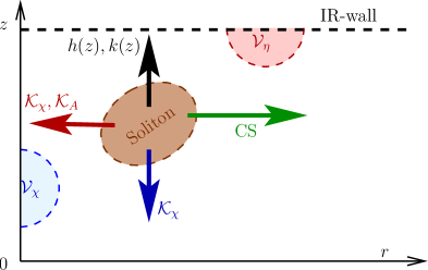
Figure 2: Schematic structure of the soliton. $\mathcal{V}_{\eta},\mathcal{V}_{\chi}$ – half-vortices of $\eta$ and $\chi$ scalars. Arrows show the effective forces produced by the metric ($h(z),k(z)$), kinetic terms of $\chi$ and $A_{\mu}$ ($\mathcal{K}_{\chi},\mathcal{K}_{A}$) and self interaction with the Abelian field in the CS-term.

At this point we see that the holographic baryon is a soliton consisting of two interacting half-vortices of two scalar fields. One is located on the IR wall and another at the center of the soliton (see Fig. 2). Now it is important to consider the energy of the solution and ensure that there exists a mechanism which stabilizes its size, preventing the soliton from collapsing.

It was pointed out in Ref. Hata:2007mb that due to the metric factors $h(z),k(z)$ the energy of the soliton is roughly inversely proportional to its $z$ position. Hence the solution tends to lie at the largest possible $z=z_{m}$. In other words, the metric provides a force, which pulls the solution to the IR wall.

On the other hand, due to the IR boundary condition on $\bm{X}$, the core of the $\chi$ vortex cannot approach IR wall too close. This would lead to a large gradient of $\chi$, which evolves from zero in the core to $\chi\sim\sigma$ on the wall. Hence the kinetic term of $\chi$ (15) and IR boundary condition (3) provide a counterforce, which repels the solution from the wall.

One can see though that this counterforce is proportional to the radius of the solution squared. Therefore it becomes negligible when the size of the soliton is small. Moreover, the whole $\chi$ energy term (15) is proportional to $r^{2}$, so it contributes (in addition to the gauge field kinetic term (13)) to the pressure, which would shrink the solution to zero size.

It is known Hata:2007mb ; Pomarol:2008aa that the important counterforce to this shrinking, which stabilizes the radius of the solution, is provided by the interaction of the soliton with the Abelian gauge field via the Chern-Simons term (18). The smaller the radius of the solution becomes, the higher the density of topological charge is, which sources the temporal component of the vector Abelian field, and the larger its gradient is. This results in the effective internal pressure which fixes the size of the soliton (see Fig. 2).

This treatment shows an interesting effect, which is produced by the chiral scalar field in the “hard-wall” model. Once the soliton radius is fixed by the CS term, the IR boundary condition (3) together with the $\chi$ kinetic term (15) produce the force which repels the soliton from the IR wall. The larger the chiral condensate is, the stronger the repulsion is. At large enough values of $\sigma$, this repulsion will define the equilibrium $z$ coordinate of the soliton center and therefore, will directly affect its energy. Hence one should expect a substantial dependence of the baryon mass on the chiral condensate. In the Sakai-Sugimoto model, though, the radius of the soliton is inversely proportional to the ’t Hooft coupling and is therefore parametrically small Hata:2007mb ; Bolognesi:2013nja . This renders the repulsive force parametrically small as well and consequently it is questionable whether in the Sakai-Sugimoto model any impact of the chiral condensate on the baryon mass can be observed.

IV Numerical solution

In order to confirm the expectations outlined above we construct the soliton solution numerically. For the numerical simulation we choose the “hard-wall” model, so the metric is unperturbed AdS₅: $h(z)=k(z)=L/z$, and the scalar asymptotic profile is given by Eq. (1). The couplings in the model have the values Erlich:2005qh ; Cherman:2008eh ; Gorsky:2009ma

$$g_{5}^{2}=\frac{12\pi^{2}}{N_{c}},\qquad g_{X}^{2}=\frac{3}{g_{5}^{2}}.$$ (23)

The IR wall is located at $z_{m}=(323\,\mathrm{MeV})^{-1}$ which is fixed by the mass of the $\rho$-meson Erlich:2005qh . The parameter $\sigma$ is related to the quark condensate as in Eq. (2). In what follows, unless explicitly stated otherwise, we will measure all the dimensional quantities in terms of $z_{m}$ and rescale the curvature radius $L=1$.

Because we are dealing with a gauge field theory, first of all we need to fix the gauge. It is useful to adopt the Lorenz gauge $\partial_{z}A_{z}+\partial_{r}A_{r}=0$. The gauge fixing condition is enforced by adding the Lagrange term to the action

$$S_{\lambda}=\bm{\lambda}\left(-\frac{4\pi}{2g_{5}^{2}}\right)r^{2}\frac{h(z)^{2}}{k(z)}\left[\partial_{z}A_{z}+\partial_{r}A_{r}\right]^{2}.$$ (24)

With this choice of gauge fixing, the equations for $A_{z}$ and $A_{r}$ become elliptic and the boundary value problem has unique solution. The resulting physical solution should not depend on the value of $\bm{\lambda}$.

Next we need to choose the boundary conditions consistently with the given gauge. In the $\eta$ half-vortex the phase $\theta$ changes by $\pi$ along the boundary of space. We can chose the gauge in such a way that the total winding occurs along the $r\rightarrow\infty$ boundary, where $\theta$ changes linearly $\theta\big{|}_{r\rightarrow\infty}=-\frac{\pi}{2}+\pi\frac{z}{z_{m}}$ and it is constant everywhere except the jump by $\pi$ in the core of the $\eta$ half-vortex on the IR boundary. This choice of $\theta$ ensures us that $\eta_{2}=-1$ at $z=0$, hence there are no source terms for the axial current, $\eta_{2}=-1$ at infinity, hence the currents decay there, and $\eta_{1}=0$ on the IR wall which is required by the IR condition (4). Due to the interaction between the scalars $\chi$ and $\eta$ (22), the phase difference $(\theta-\gamma)$ should be either $-\frac{\pi}{2}$ or $\frac{\pi}{2}$ on all the boundaries. Therefore the phase $\gamma$ winds linearly along the $r\rightarrow\infty$ boundary as well: $\gamma\big{|}_{x=1}=\pi\frac{z}{z_{m}}$. It is constant along the $z=0$ and $z=z_{m}$ boundaries, having a $\pi$ jump in the core of the $\chi$ half-vortex at $r=0$. One can check that this choice of phase guarantees the constant value of the quark mass $m$ at $z=0$.

The pure gauge condition at $r\rightarrow\infty$ will then fix $A_{z}$ to be a constant: $A_{z}\big{|}_{r\rightarrow\infty}=\partial_{z}\theta=\partial_{z}\gamma=z_{m}^{-1}\pi$. Hence according to the Lorenz gauge, we get $\partial_{r}A_{r}\big{|}_{r\rightarrow\infty}=-\partial_{z}A_{z}=0$. As we discussed in the introduction, on the IR boundary $A_{r}\big{|}_{z=z_{m}}=0$ due to the merging of the Left and Right branes at this point (4). This does not apply though to the $z$ component and thus the gauge condition will take the form $\partial_{z}A_{z}\big{|}_{z=z_{m}}=-\partial_{r}A_{r}=0$. The boundary condition on the UV boundary $z=0$ is dictated by the absence of the sources for the spatial axial current, hence $A_{r}\big{|}_{z=0}=0$ and $\partial_{z}A_{z}=-\partial_{r}A_{r}=0$. Finally in the center of the soliton the pure gauge condition states $A_{z}\big{|}_{r=0}=0$ and consequently $\partial_{r}A_{r}\big{|}_{r=0}=0$. The boundary conditions for the Abelian vector field $v$ are set by the absence of sources, regularity at the center and on the IR wall as well as the fall-off condition at infinity. Reexpressing these results in terms of the scalar fields $\eta_{\alpha},\chi_{\alpha}$ we get the set of the boundary conditions shown in Table 1, which we will use for the numerical solution. Conveniently, all of them are either of Dirichlet or of Neumann type.

$r\rightarrow\infty$		$z=0$		$r=0$		$z=z_{m}$
$\eta_{1}$ =	$\cos\big{(}-\frac{\pi}{2}+\pi\frac{z}{z_{m}}\big{)}$	$\eta_{1}$ =	$0$	$\eta_{1}$ =	$0$	$\eta_{1}$ =	$0$
$\eta_{2}$ =	$\sin\big{(}-\frac{\pi}{2}+\pi\frac{z}{z_{m}}\big{)}$	$\eta_{2}$ =	$-1$	$\eta_{2}$ =	$-1$	$\partial_{z}\eta_{2}$ =	$0$
$\chi_{1}$ =	$(mz+\sigma z^{3})\cos\big{(}\pi\frac{z}{z_{m}}\big{)}$	$\chi_{1}$ =	$(mz+\sigma z^{3})$	$\partial_{r}\chi_{1}$ =	$0$	$\chi_{1}$ =	$-(mz+\sigma z^{3})$
$\chi_{2}$ =	$(mz+\sigma z^{3})\sin\big{(}\pi\frac{z}{z_{m}}\big{)}$	$\chi_{2}$ =	$0$	$\chi_{2}$ =	$0$	$\chi_{2}$ =	$0$
$\partial_{r}A_{r}$ =	$0$	$A_{r}$ =	$0$	$\partial_{r}A_{r}$ =	$0$	$A_{r}$ =	$0$
$A_{z}$ =	$z_{m}^{-1}\pi$	$\partial_{z}A_{z}$ =	$0$	$A_{z}$ =	$0$	$\partial_{z}A_{z}$ =	$0$
$v$ =	$0$	$v$ =	$0$	$\partial_{r}v$ =	$0$	$\partial_{z}v$ =	$0$

Table 1: Boundary conditions for the fields used in the numerical calculation.

We look for a solution to the equations of motion, which follow from Eqs. (13),(17-18). In order to reduce the problem to the calculation on a square patch $[0,1]_{x}\times[0,1]_{y}$ we introduce the rescaled coordinates

$$r=c\ \mathrm{tan}\Big{(}\frac{\pi}{2}x\Big{)},\qquad z=z_{m}\ y,$$ (25)

where the dimensional constant $c$ specifies the radial scale on which the solution will be best resolved. On this patch the homogeneous grid $N_{x}\times N_{y}$ is introduced and we construct 7 equations (one for each dynamical field) on each node by the nearest neighbor discretization of the derivatives in the equations of motion.

Special attention should be paid to the boundaries $r=0,z=0$ and $r\rightarrow\infty$, as the equations of motion are divergent there. We do not perform the regularization by stepping out from the boundary. Instead, for the fields with Neumann boundary conditions, we expand the equations of motion near the singular point and solve the leading order contribution. This allows us to impose the boundary conditions directly on the boundaries.

After discretization we obtain $7\times(N_{x}-2)\times(N_{y}-2)$ algebraic equations in internal points of the grid plus $4N_{x}+4N_{y}$ equations on the boundaries and solve the resulting system both by Newton-Raphson method and the relaxation method, independently, in order to have a good check of the numeric results. The analysis of numerical accuracy is described in the Appendix.

As a starting field configuration we take the superposition of two vortices according to Fig. 2, which has unit topological charge (9). At the end of the day we were able to find solutions with a number of different parameters $\sigma$ and $m$ on the grids $60\times 60$, $120\times 120$, $240\times 240$ and observe good convergence and matching between the two methods (several other grids were used as well, see the Appendix). The procedure is run until the change in the field values on each step falls below $10^{-8}$. For the solutions we check that they do not depend on the value of the Lagrange multiplier $\bm{\lambda}$, ensuring that the gauge fixing condition (24) is fulfilled. On top of that, we check that the observables do not depend on the choice of the parameter $c$, which defines the radial coordinate transformation (25).

V Baryon mass

Before we proceed with the analysis of various baryon parameters, it is interesting to look at the general behavior of the solution. The distribution of the topological charge at various $\sigma$ is shown in Fig. 3. At very low $\sigma$ the solution is concentrated near the IR boundary and does not feel the presence of the scalar field. At intermediate values of the chiral condensate the charge distribution is pulled downwards by the scalar “repulsion force” described above. Finally, at large $\sigma$ one can see that the solution is detached completely from the IR wall and is localized at intermediate values of the holographic coordinate $z$. Another observation is the dependence of the radial coordinate of the solution on the value of the condensate. At large $\sigma$ the shrinking force produced by the scalar part of the action grows and it is harder for the CS term to stabilize the radius of the solution. All these observations are in perfect agreement with the intuition developed in Sec. III.

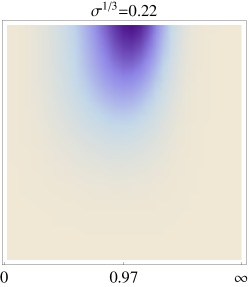
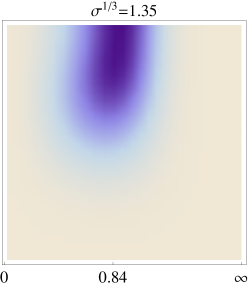
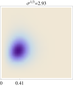
Figure 3: Topological charge density of the soliton at various values of the scalar field boundary value. At large $\sigma$ the soliton is detached from the IR wall. The radial (horizontal) coordinate and $\sigma$ are measured in units of $z_{m}=(323\ \mathrm{MeV})^{-1}$.

In order to study the mass of the holographic baryon we first regularize the energy by subtracting the infinite contribution from the vacuum configuration of the scalar field (1):

$$E_{reg}=\int dzd^{3}x\left[-\mathcal{L}+2\pi g_{X}^{2}\frac{2r^{2}}{z^{3}}\left(m^{2}-3\sigma^{2}z^{4}\right)\right].$$

The mass of the holographic baryon for different values of $\sigma$ is shown in Fig. 4 (the value of quark mass here is $m=0.01z_{m}^{-1}=3.23\,\mathrm{MeV}$ and we use $N_{c}=3$ in order to obtain the numeric results). As anticipated, at low values of $\sigma$, when the solution lies on the IR wall, the mass is governed by the confinement scale. In the opposite case of large $\sigma$, the position of the solution is only controlled by the scalar “repulsion force” and hence its mass is directly proportional to the chiral symmetry-breaking energy scale $\langle\bar{q}q\rangle^{1/3}$. The intermediate region, where the effects of chiral and confinement scales are comparable, is quite narrow, so using Eq. (2) we may approximate the result for the mass of the baryon as

$$M_{B}=N_{c}z_{m}^{-1}\, \mathrm{max}\Big{[}0.92;-0.42+0.97\ \left(2\pi^{2}\tfrac{\langle\bar{q}q\rangle}{N_{c}}\right)^{1/3}\Big{]}$$

$$=\, \mathrm{max}\Big{[}887;-407+940\ \left(z_{m}\sigma^{1/3}\right)\Big{]}\mathrm{\ MeV}.$$

It is important to check that the $N_{c}$ scaling of the baryon mass is linear due to $\langle\bar{q}q\rangle\sim N_{c}$. Interestingly, the physical value of the baryon mass $M_{B}=940\,\mathrm{MeV}$ corresponds to the point where the scalar repulsion just becomes significant (as claimed in gkk ).

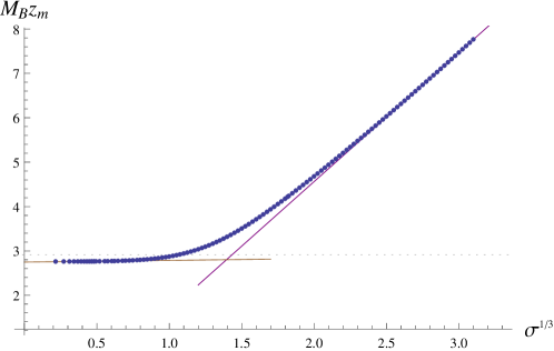
Figure 4: Dependence of the baryon mass on the chiral condensate. The solid lines show the asymptotes at small and large condensate values. The dashed line shows the physical value of the proton mass.

VI Mean values of quark operators

Now we calculate the mean values of the currents induced by the baryon. The vacuum expectation value of the operator is obtained by taking the variation of the action on the classical solution with respect to the boundary value of the corresponding field gubser-klebanov ; Bianchi:2001kw . Given the field content of the model, we are able to calculate the mean values of vector and axial quark currents as well as the scalar quark bilinear. It is important to note also that the proper formulation of the operator/field duality is possible only in a specific gauge in the 5D theory, namely in the axial gauge $A_{z}=0$. Our numerical solution was obtained in different, Lorentz gauge (24), hence a gauge transformation should be performed before we can obtain the mean values. Let us denote the fields in the axial gauge with bars: $\bar{A}_{z}=0$. The action (13) evaluated on the classical solution in axial gauge can be recast as a boundary term

$$S_{cl}=\int dtdr\ 4\pi r^{2}\ \left(-\frac{1}{g_{5}^{2}}\right)\bigg{\{}\frac{1}{z}\bar{A}_{r}\partial_{z}\bar{A}_{r}+\frac{2}{r^{2}z}\left[\bar{\eta}_{2}\partial_{z}\bar{\eta}_{2}+\bar{\eta}_{1}\partial_{z}\bar{\eta}_{1}\right]+\frac{3}{z^{3}}\left[\bar{\chi}_{1}\partial_{z}\bar{\chi}_{1}+\bar{\chi}_{2}\partial_{z}\bar{\chi}_{2}\right]\bigg{\}}_{z=\epsilon}.$$

According to the equations of motion, the solutions near the boundary are represented by the Frobenius series

$$\bar{A}_{r}=a^{(0)}+a^{(2)}z^{2}+\dots,\qquad\bar{\eta}_{\alpha}=\eta^{(0)}_{\alpha}+\eta^{(2)}_{\alpha}z^{2}+\dots,\qquad\bar{\chi}_{\alpha}=\chi^{(1)}_{\alpha}z+\chi^{(3)}_{\alpha}z^{3}+\dots.$$ (26)

Substituting these into the action we find a divergent contribution as $\epsilon\rightarrow 0$ which comes from the $\chi$ term: $S_{div}\sim\epsilon^{-2}\big{(}\chi_{\alpha}^{(1)}\big{)}^{2}$. This must be regularized according to the holographic regularization procedure Bianchi:2001kw with a boundary counter term

$$S_{c.t.}=\int dtdr\ 4\pi r^{2}\left(\frac{3}{g_{5}^{2}}\right)\frac{1}{\epsilon^{4}}\left[\bar{\chi}_{1}(\epsilon)^{2}+\bar{\chi}_{2}(\epsilon)^{2}\right].$$ (27)

In order to get the mean value of the 3D spatial current, one needs to take the variation of the regularized action $S_{reg}=S_{cl}+S_{c.t.}$ with respect to the boundary value of the corresponding spatial component of the 3D vector field $A^{(0)}_{i}$ or $V^{(0)}_{i}$. It is convenient to express these boundary values in terms of the 2D fields of the ansatz (11). This will reduce the problem to the variations with respect to $\eta_{\alpha}^{(0)},\chi_{\alpha}^{(1)}$ and $a^{(0)}$. Therefore in terms of the Frobenius coefficients (26) we get

$$\langle J^{V}\rangle^{a}_{i} =-\frac{2}{g_{5}^{2}}\frac{\eta_{2}^{(2)}}{r}\ \epsilon_{iak}\frac{x_{k}}{r},$$ (28)

$$\langle J^{A}\rangle^{a}_{i} =-\frac{2}{g_{5}^{2}}\left[\frac{\eta_{1}^{(2)}}{r}\ \left(\delta_{ia}-\frac{x_{i}x_{a}}{r^{2}}\right)+a^{(2)}\ \frac{x_{i}x_{a}}{r^{2}}\right],$$

$$\langle\bar{q}q\rangle_{\rho\gamma} =-\frac{6}{g_{5}^{2}}\left[\chi_{1}^{(3)}\ \frac{\mathbbm{1}}{2}+i\chi_{2}^{(3)}\ \frac{x^{a}t^{a}}{r}\right]_{\rho\gamma}.$$

The values of the coefficients can be calculated after we transform the numerical solution to the axial gauge. With the gauge function $\lambda$, the fields in Eq. (13) transform as

$$\bar{A}=A+\partial\lambda,\qquad\bar{\eta}_{\alpha}=\eta_{\alpha}\cos\lambda-\epsilon^{\alpha\beta}\eta_{\beta}\sin\lambda,\qquad\bar{\chi}_{\alpha}=\chi_{\alpha}\cos\lambda-\epsilon^{\alpha\beta}\chi_{\beta}\sin\lambda.$$ (29)

In order to reach the axial gauge $\bar{A}_{z}=0$ while keeping the value of the quark mass $m\sim\chi_{1}^{(1)}$ constant, we choose

$$\lambda=-\int_{0}^{z_{m}}dzA_{z}.$$ (30)

In the vicinity of the boundary, it is expanded as $\lambda(\epsilon)=-\epsilon A_{z}(\epsilon)$. At the end of the day the coefficients in Eq. (28) are expressed in terms of the components of our numerical solution

$$\chi_{\alpha}^{(3)} =\left.\frac{1}{2z}\partial_{z}\frac{\bar{\chi}_{\alpha}}{z}\right|_{z=\epsilon}=\frac{1}{2}\left[\frac{1}{z}\mathcal{D}_{z}\Big{(}\frac{\chi_{\alpha}}{z}\Big{)}+\epsilon^{\alpha\beta}A_{z}\,\mathcal{D}_{z}\Big{(}\frac{\chi_{\beta}}{z}\Big{)}\right]_{z=\epsilon},$$ (31)

$$\eta_{\alpha}^{(2)} =\left.\frac{1}{2z}\partial_{z}\bar{\eta}_{\alpha}\right|_{z=\epsilon}=\frac{1}{2}\left[\frac{1}{z}\mathcal{D}_{z}\eta_{\alpha}+\epsilon^{\alpha\beta}A_{z}\,\mathcal{D}_{z}\eta_{\beta}\right]_{z=\epsilon},$$

$$a^{(2)} =\left.\frac{1}{2z}\partial_{z}\bar{A}_{r}\right|_{z=\epsilon}=\frac{1}{2}\left[\frac{1}{z}(\partial_{z}A_{r}-\partial_{r}A_{z})\right]_{z=\epsilon}.$$

Given these expressions we can calculate the mean values of the currents (28).

It is interesting to study the local scalar VEV. In a hedgehog Skyrmion it behaves as

$$\langle\bar{q}q\rangle(r)=\langle\bar{q}q\rangle_{0}\left(\cos(\theta)+i\frac{t^{a}x^{a}}{r}\sin(\theta)\right),$$ (32)

where $\langle\bar{q}q\rangle_{0}$ is the value of the chiral condensate at infinity, and $\theta(r)$ is a chiral phase which goes from $\pi$ in the center of the Skyrmion to 0 at infinity. In the analysis of our solution we find that the phase of the scalar VEV behaves exactly as expected (see Fig. 5), but on top of that, the modulus of the chiral condensate is suppressed in the center of the baryon. This observation agrees with the lattice studies Iritani:2014fga of the partial chiral symmetry restoration inside baryons. Spectacularly, while the value of the chiral condensate affects the baryon mass, the presence of thee baryon has its effect on the scalar quark density as well.

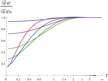
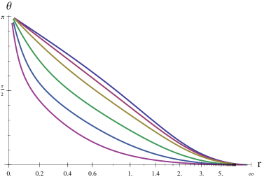
Figure 5: Relative local mean value of the scalar operator $\langle\bar{q}q\rangle$ and its phase $\theta$ for various solutions with $\sigma^{1/3}z_{m}=\{0.31,\ 0.37,\ 0.62,\ 1.50,\ 2.10,\ 3.10\}$ counting from top to bottom.

The other interesting observable is the nucleon axial charge $g_{A}$. In Refs. Panico:2008it ; Domenech:2010aq the value of the axial charge calculated for a holographic baryon was almost 2 times smaller than the phenomenological value $g_{A}\sim 1.25$, although the other baryon observables exhibited good agreement. One should expect, though, the dependence of $g_{A}$ on the pion mass, which is related to the chiral condensate by the Gell-Mann-Oakes-Renner relation. Thus it is interesting to check whether this value changes significantly for different values of $\sigma$. For this purpose we reproduce the calculation of Ref. Domenech:2010aq and study the dependence of $g_{A}$ on the chiral condensate. If one parametrize the mean value of the QCD axial quark current by the following radial functions

$$\langle J^{A}\rangle_{i}^{a}(\mathbf{r}) =A_{1}(r)\delta^{ia}+A_{2}(r)\frac{x^{i}x^{a}}{r^{2}},$$ (33)

the axial form factor is expressed as mei

$$G_{A}(q^{2})=-\left(\frac{M_{B}}{E}\right)\frac{8\pi}{3}\int\limits_{0}^{\infty}\left[r^{2}j_{0}(qr)A_{1}(r)+\Big{(}\frac{r}{q}\Big{)}j_{1}(qr)A_{2}(r)\right],$$

and the axial vector charge $g_{A}$ is

$$g_{A} =G_{A}(\mathbf{q}^{2}=0)=-\frac{8\pi}{3}\int\limits_{0}^{\infty}dr\,r^{2}\left[A_{1}(r)+\tfrac{1}{3}A_{2}(r)\right].$$ (34)

The values of $g_{A}$ for different $\sigma$s and different quark masses $m$ are shown in Fig. 6 (for details of the numerical calculation see the Appendix). At $\sigma^{1/3}=1.23$ (which provides a good fit to QCD phenomenology) we get $g_{A}=0.63$, which is close to the value obtained in Ref. Domenech:2010aq . The axial charge exhibits only a minor dependence on the parameters of chiral symmetry breaking. So we can conclude that the discrepancy with phenomenological value is a qualitative feature and can not be cured by a simple tuning of the model. We note that this result is similar to the Skyrme model, where $g_{5}$ also has a small value Adkins:1983ya , which is weakly affected by the pion mass. The problem of small $g_{A}$ is a long standing problem in Skyrmion physics. There might be significant $N_{c}$ corrections to this value, which are not taken into account here and may require a qualitative modification of the model. For a detailed discussion of this issue see e.g. Panico:2008it ; mei and references therein.

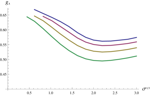
Figure 6: The baryon axial charge for various $\sigma$s and various quark masses: from top to bottom $mz_{m}=\{0.01,0.02,0.04,0.08\}$ ($z_{m}^{-1}=323\,\mathrm{MeV}$).

VII Conclusion

In this paper we have studied the interplay between chiral symmetry breaking and the baryon in a holographic QCD setup. Although the numerical calculations were done for a specific “hard-wall” model, our qualitative treatment is fairly general and the results should hold for a generic model. We have proved in a clear-cut manner the conjecture advocated in Refs. gk ; gkk that there are essentially two regimes in baryon physics where the dependence of the baryon mass on the chiral condensate is very different. The numerical calculations show that the physical value of the baryon mass is in the transition region between the two regimes, which clearly demonstrates that the Ioffe’s formula for the baryon mass ioffe derived in QCD sum rules is relevant.

The main finding of our work is the phenomenon of repulsion of the baryon from the IR wall due to the interaction with the scalar field dual to the chiral condensate. It is very important to understand how this repulsion looks from the perspective of the Sakai-Sugimoto setup. At large values of the chiral condensate the baryon is moved away from the tip of the cigar. The only way to do this without violating P-symmetry is to split the soliton into two symmetric halves. One of them is moved to the Left brane and another to the Right one. For symmetry reasons, these two halves carry equal half-integer baryon charges and opposite half-integer Abelian axial charges, producing in total the solution with unit baryon charge.

In spirit the splitting of the holographic baryon is very similar to the splitting of an instanton on compact space into monopoles. This phenomenon takes place when the system is considered at finite temperature or finite chemical potential. However, the details can be very different and deserve a thorough study. In particular it is not completely clear how the splitting occurs in terms of the branes. The baryon is represented by the D4 brane wrapped around the internal sphere $S^{4}$ and cannot be naively split into half D4 branes. The process could be viewed upon a T-duality transformation around the compact coordinate on the cigar. Another delicate issue concerns the behavior at the nonvanishing temperature. Different scenarios of the splitting phenomenon could take place once one takes into account the temperature dependence of the chiral condensate.

We should recall, that once one moves from the tip of the cigar, the separation between $D8$ and $\overline{D8}$ branes grows with the radius of the compact circle $\tau$. In our treatment we neglected this separation in favor of the opportunity of working with the 5D model with local fields, but in a general setup once the baryon is split and repelled from the tip of the cigar this separation may lead to interesting phenomena. For example, although the net Abelian axial charge of the solution is zero, the axial dipole moment is nonzero and proportional to the size of the $\tau$-circle. The $\theta$- dependence of the Skyrmion due to the splitting can be considered in the SS model as well since the $\theta$-term corresponds to the holonomy of the one-form RR field along the compact coordinate on the cigar. One should note though, that the splitting effect is proportional to the size of the instanton and therefore is parametrically suppressed by the ’t Hooft coupling in the original Sakai-Sugimoto model. On the other hand, the divergent tachyonic mode of the open string can provide a sufficiently large scalar boundary value, which will render the effect sizable. Given these subtleties, it is not clear in which particular setup one should study the phenomena mentioned above.

The other interesting finding, that we made in the present study, is the backreaction of the baryon solution on the local density of the quark bilinear operator. We find that the chiral condensate gets suppressed inside the baryon and the chiral symmetry is partially restored. This idea was widely discussed in the literature but to our knowledge this phenomenon has not been directly observed in any models of QCD. The chiral condensate in the SS model follows from tachyon condensation on the string, hence it would be interesting to investigate the impact of the Skyrmion on the tachyon action directly. This could also be related to the recent discussion of the spectrum of hadrons including baryons in terms of the details of the Dirac operator spectrum in QCD glozman .

Appendix A Accuracy of the numerical calculation

We perform our numerical analysis using two different methods implemented in different codes in order to exclude any possible systematic errors (see text). The mass and topological charge distribution of the soliton is calculated on the grids $60\times 60$, $120\times 120$ and $240\times 240$. One can observe a good convergence of the results (see Fig. 7) and the estimated precision of the finest grid is within 1%.

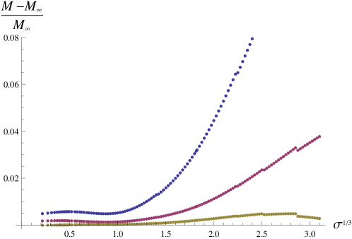
Figure 7: The accuracy of calculated baryon mass on different $N\times N$ grids with $N=\{60,120,240\}$ (from top to bottom). $M_{\infty}$ is the extrapolated value for $N\rightarrow\infty$.

It is numerically challenging to calculate the axial charge (34). The mean value of the axial current is defined by the asymptotic form of the solution near the boundary $y=\epsilon\rightarrow 0$. The equations of motion are singular on this boundary, hence the precision of the calculated solution should be higher than $\epsilon$. On top of that, the integrand in Eq. (34) has several factors of $r$ and in order to get finite results one needs to ensure that the fall off of the solution at large $r$ is calculated with a precision of order $1/r^{2}$. An additional difficulty is the fact that we impose nontrivial boundary conditions at $r\rightarrow\infty$. Because of that, the accuracy of the solution at $r\rightarrow\infty$ is limited by the precision of the finite difference approximation of the scalar field derivatives on the grid. At the end of the day we are forced to use very dense grids in the $z$ direction in order to obtain convergent integrals for $g_{A}$. The sample of the integrand in Eq. (34) for $\sigma=2.6$ and $m=0.01$ calculated on the grids $60\times 120$, $60\times 240$, $60\times 480$ and $60\times 1000$ is shown in Fig. 8. While for intermediate values of $x$, the results of all the grids coincide, the tail at $x=1$ ($r\rightarrow\infty$) is resolved only on the finest one.

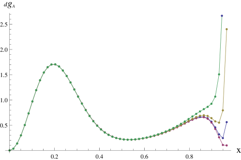
Figure 8: The integrand (34) calculated for $\sigma=2.6$ on different grids with $N_{y}=\{120,240,480,1000\}$ (from top to bottom). The tail is decently resolved only on the finest grid.

References

- (1) H. Hata, T. Sakai, S. Sugimoto and S. Yamato, Prog. Theor. Phys. 117, 1157 (2007) [hep-th/0701280].
- (2) S. Bolognesi and P. Sutcliffe, JHEP 1401, 078 (2014) [arXiv:1309.1396 [hep-th]].
- (3) M. Rozali, J. B. Stang and M. van Raamsdonk, JHEP 1402, 044 (2014) [arXiv:1309.7037 [hep-th]].
- (4) K. Hashimoto, T. Sakai and S. Sugimoto, Prog. Theor. Phys. 120, 1093 (2008) [arXiv:0806.3122 [hep-th]].
- (5) D. K. Hong, M. Rho, H. U. Yee and P. Yi, Phys. Rev. D 77, 014030 (2008) [arXiv:0710.4615 [hep-ph]].
- (6) K. Y. Kim and I. Zahed, JHEP 0809, 007 (2008) [arXiv:0807.0033 [hep-th]].
- (7) V. Kaplunovsky, D. Melnikov and J. Sonnenschein, JHEP 1211, 047 (2012) [arXiv:1201.1331 [hep-th]].
- (8) A. Dymarsky, D. Melnikov and J. Sonnenschein, JHEP 1106, 145 (2011) [arXiv:1012.1616 [hep-th]].
- (9) M. Rho, S. J. Sin and I. Zahed, Phys. Lett. B 689, 23 (2010) [arXiv:0910.3774 [hep-th]].
- (10) O. Domenech, G. Panico and A. Wulzer, Nucl. Phys. A 853, 97 (2011) [arXiv:1009.0711 [hep-ph]].
- (11) B. L. Ioffe, Nucl. Phys. B 188, 317 (1981) [Erratum-ibid. B 191, 591 (1981)].
- (12) T. Sakai and S. Sugimoto, Prog. Theor. Phys. 113, 843 (2005) [hep-th/0412141].
- (13) T. Sakai and S. Sugimoto, Prog. Theor. Phys. 114, 1083 (2005) [hep-th/0507073].
- (14) E. Witten, Adv. Theor. Math. Phys. 2, 505 (1998) [hep-th/9803131].
- (15) S. Seki and J. Sonnenschein, JHEP 0901 (2009) 053 [arXiv:0810.1633 [hep-th]].
- (16) O. Bergman, S. Seki and J. Sonnenschein, JHEP 0712, 037 (2007) [arXiv:0708.2839 [hep-th]].
- (17) A. Dhar and P. Nag, Phys. Rev. D 78, 066021 (2008) [arXiv:0804.4807 [hep-th]].
- (18) J. Erlich, E. Katz, D. T. Son and M. A. Stephanov, Phys. Rev. Lett. 95, 261602 (2005) [hep-ph/0501128].
- (19) A. Karch, E. Katz, D. T. Son and M. A. Stephanov, Phys. Rev. D 74, 015005 (2006) [hep-ph/0602229].
- (20) S. S. Gubser, I. R. Klebanov, A. M. Polyakov, Phys. Lett. B428, 105-114 (1998). [hep-th/9802109].
- (21) A. Krikun, Phys. Rev. D 77, 126014 (2008) [arXiv:0801.4215 [hep-th]].
- (22) A. Gorsky and A. Krikun, Phys. Rev. D 79, 086015 (2009) [arXiv:0902.1832 [hep-ph]].
- (23) A. Cherman, T. D. Cohen and E. S. Werbos, Phys. Rev. C 79, 045203 (2009) [arXiv:0804.1096 [hep-ph]].
- (24) A. Pomarol and A. Wulzer, Nucl. Phys. B 809, 347 (2009) [arXiv:0807.0316 [hep-ph]].
- (25) A. Gorsky and A. Krikun, Phys. Rev. D 86, 126005 (2012) [arXiv:1206.4515 [hep-th]].
- (26) A. Gorsky, P. N. Kopnin and A. Krikun, Phys. Rev. D 89, no. 2, 026012 (2014) [arXiv:1309.3362 [hep-th]].
- (27) E. Witten, Phys. Rev. Lett. 38, 121 (1977).
- (28) Wolfram Research, Inc., Mathematica, Version 9.0, Champaign, IL (2013).
- (29) M. Bianchi, D. Z. Freedman and K. Skenderis, Nucl. Phys. B 631, 159 (2002) [hep-th/0112119].
- (30) T. Iritani, G. Cossu and S. Hashimoto, arXiv:1412.2322 [hep-lat].
- (31) G. Panico and A. Wulzer, Nucl. Phys. A 825, 91 (2009) [arXiv:0811.2211 [hep-ph]].
- (32) U. G. Meissner, Phys. Rept. 161, 213 (1988).
- (33) G. S. Adkins, C. R. Nappi and E. Witten, Nucl. Phys. B 228, 552 (1983).
- (34) L. Y. Glozman, C. B. Lang and M. Schrock, Phys. Rev. D 86, 014507 (2012) [arXiv:1205.4887 [hep-lat]].