Diffusive cosmic ray acceleration at relativistic shock waves with magnetostatic turbulence

Abstract

The analytical theory of diffusive cosmic ray acceleration at parallel stationary shock waves with magnetostatic turbulence is generalized to arbitrary shock speeds $V_{s}=\beta_{1}c$, including in particular relativistic speeds. This is achieved by applying the diffusion approximation to the relevant Fokker-Planck particle transport equation formulated in the mixed comoving coordinate system. In this coordinate system the particle’s momentum coordinates $p$ and $\mu=p_{\parallel}/p$ are taken in the rest frame of the streaming plasma, whereas the time and space coordinates are taken in the observer’s system. For magnetostatic slab turbulence the diffusion-convection transport equation for the isotropic (in the rest frame of the streaming plasma) part of the particle’s phase space density is derived. For a step-wise shock velocity profile the steady-state diffusion-convection transport equation is solved. For a symmetric pitch-angle scattering Fokker-Planck coefficient $D_{\mu\mu}(-\mu)=D_{\mu\mu}(\mu)$ the steady-state solution is independent of the microphysical scattering details. For nonrelativistic mono-momentum particle injection at the shock the differential number density of accelerated particles is a Lorentzian-type distribution function which at large momenta approaches a power law distribution function $N(p\geq p_{c})\propto p^{-\xi}$ with the spectral index $\xi(\beta_{1})=1+[3/(\Gamma_{1}\sqrt{r^{2}-\beta_{1}^{2}}-1)(1+3\beta_{1}^{2})]$. For nonrelativistic ($\beta_{1}\ll 1$) shock speeds this spectral index agrees with the known result $\xi(\beta_{1}\ll 1)\simeq(r+2)/(r-1)$, whereas for ultrarelativistic ($\Gamma_{1}\gg 1$) shock speeds the spectral index value is close to unity.

1. Introduction

One of the most important problems of modern astrophysics is to explain how cosmic ray particles are accelerated to relativistic energies in powerful sources of nonthermal radiation. Diffusive first-order Fermi acceleration at nonrelativistic shock fronts has been regarded as a prime candidate for particle acceleration in astrophysics (for reviews see Drury 1983; Blandford and Eichler 1987). Modern TeV air-Cherenkov telescopes have indeed resolved the shock regions in supernova remnants and identied the shocks as strong emission regions of TeV photons generated by the accelerated particles (Hinton and Hofmann 2009).

It is likely that diffusive shock acceleration also operates efficiently at magnetized shock waves with relativistic speeds. Such relativistic shocks form during the interaction of relativistic supersonic and super-Alfvenic outflows with the ambient ionized interstellar or intergalactic medium (Gerbig and Schlickeiser 2009) producing anisotropic counterstream plasma distribution functions due to shock-reflected charged particles in the upstream medium (Spitkovsky 2008, Sironi and Spitkovsky 2009). Relativistic outflows are a direct consequence of violent explosive events such as in gamma-ray burst sources (Piran 1999) both in the collapsar (Woosley 1993, Paczynski 1998) and supranova (Vietri and Stella 1998) models, but also occur as highly collimated pulsar winds and jets of active galactic nuclei with initial bulk Lorentz factors $\Gamma_{0}=(1-(V_{0}/c)^{2})^{-1/2}\simeq 400$.

The transport and acceleration of energetic particles in the partially turbulent cosmic magnetic fields associated with shocks is described using the Fokker-Planck equation for the particle distribution function (for a recent derivation, see Schlickeiser 2011). The diffusion approximation for the particle density in the rest frame of the fluid is a well-known simplied form of the Fokker-Planck equation, which results when turbulent pitch-angle scattering is strong enough to ensure that the scale of the particle density variation is signicantly greater than the particle mean free path (Jokipii 1966, Hasselmann and Wibberenz 1968, Earl 1974). Numerical studies confirmed the accuracy of the diffusion approximation in a uniform mean guide magnetic field (Kota et al. 1982).

While for nonrelativistic shock waves the analytic theory of diffusive shock acceleration is well developed (Axford et al. 1977, Krymsky 1987, Blandford and Ostriker 1978, Bell 1978, Drury 1983), for relativistic shock speeds such an analytical theory does not exist sofar even for parallel shock waves, although the underlying Fokker-Planck transport equation (see Eq. (3) below) for the particle dynamics has already been derived (Webb 1985; Kirk, Schneider and Schlickeiser 1988) some years ago. The existing literature concentrated on semi-numerical eigenfunction solutions of this Fokker-Planck transport equation pioneered by Kirk and Schneider (1987), relativistic Monte Carlo simulations (Ellison et al. 1990, Ostrowski 1991, Bednarz and Ostrowski 1998, Summerlin and Baring 2012), and relativistic particle in-cell simulations (Spitkovsky 2008, Sironi and Sptkovsky 2009). It is the purpose of this manuscript to develop an analytical study of cosmic ray acceleration in parallel relativistic magnetized shock waves employing the diffusion approximation in the upstream and downstream regions of the shock wave. The development runs much in parallel with the existing work on nonrelativistic shocks.

2. Basic equations

Magnetized space plasmas such as the interstellar medium harbour low-frequency linear ($\delta B\ll B_{0}$) transverse MHD waves (such as shear Alfven and magnetosonic plasma waves) with dispersion relations $\omega_{R}^{2}=V_{A}^{2}k_{\parallel}^{2}$ and $\omega_{R}^{2}=V_{A}^{2}k^{2}$, respectively, in the rest frame of the moving plasma. Faraday${}^{{}^{\prime}}$s induction law then indicates for MHD waves that the strength of turbulent electric fields $\delta E=(V_{A}/c)\delta B\ll\delta B$ is much smaller than the strength of turbulent magnetic fields. The ordering $B_{0}\gg\delta B\gg\delta E$ corresponds to the derivation of cosmic ray transport equations for $<f>(\vec{X},p,\mu,\phi,t)\to f_{0}(\vec{X},p,\mu,t)\to F(\vec{X},p,t)$ from the collisionfree Boltzmann equation fir the full phase space distribution $<f>(\vec{X},p,\mu,\phi,t)$ to the Fokker-Planck equation for its gyrotropic part $f_{0}(\vec{X},p,\mu,t)$, and to the diffusion-convection transport equation for its isotropic part $F(\vec{X},p,t)$, respectively (for a recent review see Schlickeiser 2011). Accordingly, the cosmic ray anisotropy, defined as the deviation

$$g(\vec{X},v,\mu,t)=f_{0}(\vec{X},p,\mu,t)-F(\vec{X},p,t),$$ (1)

then is small ($|g|\ll F$) with respect to $F$. The diffusion approximation applied to the Fokker-Planck transport equation for $f_{0}(\vec{X},p,\mu,t)$ allows us to relate the cosmic ray anisotropy $g$ to the solutions of the diffusion-convection tranport equation for $F$.

Because of the gyrorotation of the cosmic ray particles in the uniform magnetic field, one is not so much interested in their actual position as in the coordinates of the cosmic ray guiding center

$$\vec{X}=(X,Y,Z)=\vec{x}+{c\over q_{a}B_{0}^{2}}\vec{p}\times\vec{B}_{0}=\vec{x}+{c\over q_{a}B_{0}}\begin{pmatrix}p_{y}\\ -p_{x}\\ 0\end{pmatrix},$$ (2)

where we orient the large-scale guide magnetic field, which is uniform on the scales of the cosmic ray particles gyradii $R_{L}=v/|\Omega|$, $\vec{B}_{0}=B_{0}\vec{e}_{z}=(0,0,B_{0})$ along the $z$-axis. $v$ and $\Omega_{a}=q_{a}B_{0}/\gamma m_{a}c$ denote the speed and the relativistic gyrofrequency of a cosmic ray particle with mass $m$, charge $g_{a}$ and energy $\gamma m_{a}c^{2}$.

The Larmor-phase averaged Fokker-Planck transport equation in a medium, propagating with the stationary bulk speed $\vec{U}=U(z)\vec{e_{z}}$ with $\Gamma=[1-(U^{2}/c^{2})]^{-1/2}$ aligned along the magnetic field direction is given by (Webb 1985; Kirk, Schneider and Schlickeiser 1988)

$$\Gamma\left[1+{Uv\mu\over c^{2}}\right]{\partial f_{0}\over\partial t}+\Gamma\left[U+v\mu\right]{\partial f_{0}\over\partial z}+{v(1-\mu^{2})\over 2L}{\partial f_{0}\over\partial\mu}$$

$$-\alpha(z)\left(\mu+{U\over v}\right)\left[\mu p{\partial f_{0}\over\partial p}+(1-\mu^{2}){\partial f_{0}\over\partial\mu}\right]+{\cal R}f_{0}-S(\vec{X},p,t)$$

$$={\partial\over\partial\mu}\left[D_{\mu\mu}{\partial f_{0}\over\partial\mu}+D_{\mu\sigma}{\partial f_{0}\over\partial y_{\sigma}}\right]$$

$$+p^{-2}{\partial\over\partial y_{\omega}}p^{2}\left[D_{\omega\mu}{\partial f_{0}\over\partial\mu}+D_{\omega\sigma}{\partial f_{0}\over\partial y_{\sigma}}\right],$$ (3)

irrespective of how the Fokker-Planck coefficients are calculated, either by quasilinear (Schlickeiser 2002) or nonlinear (Shalchi 2009) cosmic ray transport theories. $\alpha(z)$ denotes the rate of adiabatic deceleration/acceleration in relativistic flows

$$\alpha(z)={c^{2}\over U(z)}{d\Gamma(z)\over dz}={dU\over dz}\Gamma^{3}={d(U\Gamma)\over dz}$$ (4)

In the Fokker-Planck Eq. (3) the phase space coordinates have to be taken in the mixed comoving coordinate system (time and space coordinates in the laboratory (=observer) system and particle’s momentum coordinates $p$ and $\mu=p_{\parallel}/p$ in the rest frame of the streaming plasma). Moreover, in Eq. (3) we use the Einstein sum convention for indices, and $y_{\omega},y_{\sigma}\in[p,X,Y]$ represent the three phase space variables with non-vanishing stochastic fields $\delta\vec{E}$ and $\delta\vec{B}$. Consequently, the term on the right-hand side generally represents 9 different Fokker-Planck coefficients: but, depending on the turbulent fields considered, not all of them are non-zero and some are much larger than others. $S(\vec{X},p,t)$ accounts for additional sources and sinks of particles.

The focusing length (Roelof 1969)

$$L=-{B_{0}^{2}\over\vec{B}_{0}\cdot\hbox{grad}\,(|\vec{B}_{0}|)}=-{B_{0}(z)\over(dB_{0}(z)/dz)}$$ (5)

represents the spatial gradient of the guide magnetic field $B_{0}$. It is the only term, resulting from the mirror force in the large scale inhomogeneous guide magnetic field, that we consider (neglecting possible drift effects). $L>0$ for a diverging guide magnetic field; $L<0$ for a converging guide magnetic field.

$${\cal R}f=-p^{-2}{\partial\over\partial p}\left[p^{2}\dot{p}_{\rm loss}f\right]+{f\over T_{c}}$$ (6)

represents continuous ($\dot{p}_{\rm loss}$) and catastrophic ($T_{c}$) momentum losses of cosmic ray particles.

For spatially constant flows the rate of adiabatic deceleration/acceleration (4) vanishes, and the remaining flow velocity ($U$) dependent terms in Eq. (3) simply result from the Lorentz transformation of special relativity of the laboratory-frame position-time coordinates $(z,t)$ to the mixed-comoving-frame position-time coordinates $(z^{{}^{\prime}},t^{{}^{\prime}})$. However, for spatially varying flow speeds $U(z)$ special relativity no longer applies and has to be replaced by the transformation laws from general realtivity. As noted by Riffert (1986) as well as Kirk, Schneider and Schlickeiser (1988) these introduce connection coefficients or Christoffel symbols of the first kind. In a flat Euclidean space-time metric the terms proportional to $\alpha(z)$ in Eq. (3) are exactly these connection coefficients.

3. Magnetostatic slab turbulence

As important special case we consider magnetostatic (vanishing turbulent electric fields), isospectral, slab ($k_{\perp}=0$) turbulence. Then the only nonvanishing Fokker-Planck coefficient is $D_{\mu\mu}$. In this case the Fokker-Planck transport equation (3) simplifies to

$$\Gamma\left[1+{Uv\mu\over c^{2}}\right]{\partial f_{0}\over\partial t}+\Gamma\left[U+v\mu\right]{\partial f_{0}\over\partial z}+{v(1-\mu^{2})\over 2L}{\partial f_{0}\over\partial\mu}$$

$$-\alpha(z)\left(\mu+{U\over v}\right)\left[\mu p{\partial f_{0}\over\partial p}+(1-\mu^{2}){\partial f_{0}\over\partial\mu}\right]+{\cal R}f_{0}$$

$$=S(\vec{X},p,t)+{\partial\over\partial\mu}\left[D_{\mu\mu}{\partial f_{0}\over\partial\mu}\right]$$ (7)

Due to the rapid pitch angle scattering the gyrotropic particle distribution function $f_{0}(\vec{X},p,\mu,t)$ adjusts very quickly to a distribution function which is close to the isotropic distribution in the rest frame of the moving background plasma. Defining the isotropic part of the phase space density $F(\vec{X},z,p,t)$ as the $\mu$-averaged phase space density

$$F(\vec{X},p,t)\equiv{1\over 2}\int_{-1}^{1}d\mu\;f_{0}(\vec{X},p,\mu,t),$$ (8)

we follow the analysis of Jokipii (1966) and Hasselmann and Wibberenz (1968) to split the total density $f_{0}$ into the isotropic part $F$ and an anisotropic part $g$,

$$f_{0}(\vec{X},p,\mu,t)=F(\vec{X},p,t)+\;g(\vec{X},p,\mu,t)$$ (9)

where because of Eq. (8)

$$\int_{-1}^{1}d\mu\,g(\vec{X},p,\mu,t)=0$$ (10)

Inserting the ansatz (9) yields for the Fokker-Planck equation (7)

$$\Gamma\left[1+{Uv\mu\over c^{2}}\right]\left({\partial F\over\partial t}+{\partial g\over\partial t}\right)+\Gamma\left[U+v\mu\right]\left({\partial F\over\partial z}+{\partial g\over\partial z}\right)$$

$$-\alpha(z)\left(\mu+{U\over v}\right)\left[\mu p{\partial F\over\partial p}+\mu p{\partial g\over\partial p}+(1-\mu^{2}){\partial g\over\partial\mu}\right]$$

$$+{v(1-\mu^{2})\over 2L}{\partial g\over\partial\mu}+{\cal R}F+{\cal R}g-S(\vec{X},p,t)={\partial\over\partial\mu}\left[D_{\mu\mu}{\partial g\over\partial\mu}\right]$$ (11)

Averaging this equation over $\mu$, using that $D_{\mu\mu}(\mu=\pm 1)=0$, leads to the diffusion-convection transport equation

$$\Gamma\left[{\partial F\over\partial t}+U{\partial F\over\partial z}\right]-{\alpha\over 3}p{\partial F\over\partial p}+{\cal R}F-S(\vec{X},p,t)$$

$$+{v\over 2}\left[\Gamma\left({\partial\over\partial z}+{U\over c^{2}}{\partial\over\partial t}\right)+{1\over L}\right]\int_{-1}^{1}d\mu\,\mu g$$

$$-{\alpha U\over 2v}\left[p{\partial\over\partial p}+2\right]\int_{-1}^{1}d\mu\,\mu g-{\alpha\over 2}\left[p{\partial\over\partial p}+3\right]\int_{-1}^{1}d\mu\,\mu^{2}g=0,$$ (12)

involving the first and second moment of the anisotropy.

Subtracting Eq. (12) from the Fokker-Planck equation (11) provides

$$\Gamma v\mu\left({\partial F\over\partial z}+{U\over c^{2}}{\partial F\over\partial t}\right)+\Gamma v\mu\left({\partial g\over\partial z}+{U\over c^{2}}{\partial g\over\partial t}\right)+\Gamma\left({\partial g\over\partial t}+U{\partial g\over\partial z}\right)$$

$$+{\alpha\over 3}p{\partial F\over\partial p}+{\cal R}g-\alpha\left(\mu+{U\over v}\right)\left[\mu p{\partial F\over\partial p}+\mu p{\partial g\over\partial p}+(1-\mu^{2}){\partial g\over\partial\mu}\right]$$

$$-\left[{v\Gamma\over 2}\left({\partial\over\partial z}+{U\over c^{2}}{\partial\over\partial t}\right)+{v\over 2L}\right]\int_{-1}^{1}d\mu\,\mu g$$

$$+{\alpha U\over 2v}\left[p{\partial\over\partial p}+2\right]\int_{-1}^{1}d\mu\,\mu g+{\alpha\over 2}\left[p{\partial\over\partial p}+3\right]\int_{-1}^{1}d\mu\,\mu^{2}g$$

$$+{v(1-\mu^{2})\over 2L}{\partial g\over\partial\mu}={\partial\over\partial\mu}\left[D_{\mu\mu}{\partial g\over\partial\mu}\right]$$ (13)

We note that Eqs. (12) and (13) are still exact.

3.1. Diffusion approximation for cosmic shock waves

With $|g|\ll F$ we approximate the anisotropy equation (13) to leading order by

$$\Gamma v\mu\left({\partial F\over\partial z}+{U\over c^{2}}{\partial F\over\partial t}\right)+\alpha\left[{1\over 3}-\mu^{2}-{U\mu\over v}\right]p{\partial F\over\partial p}$$

$$\simeq{\partial\over\partial\mu}\left[D_{\mu\mu}{\partial g\over\partial\mu}\right]$$ (14)

In previous nonrelativistic ($\Gamma\simeq 1$) studies (Jokipii 1966, Hasselmann and Wibberenz 1968, Schlickeiser et al. 2007, Schlickeiser and Shalchi 2008) only the first term on the left-hand side of Eq. (14) has been considered, so that

$$v\mu{\partial F\over\partial z}\simeq{\partial\over\partial\mu}\left[D_{\mu\mu}{\partial g\over\partial\mu}\right]$$ (15)

For gradual flows with non-zero values of $\alpha$ for an extended region of space, we have to consider also the term resulting from the momentum gradient $(\partial F/\partial p)$. This case will be considered elsewhere.

Here we consider flows with non-zero values of $\alpha$ in a very limited region of space such as cosmic shock waves. We chose as laboratory frame the rest frame of the shock wave with the step-wise velocity profile

$$U(z)=\begin{cases}-U_{1}=\hbox{const.}&\text{for $0<z\leq\infty$}\;\hbox{(upstream)}\\ -U_{2}=\hbox{const.}&\text{for $-\infty\leq z<0$}\;\hbox{(downstream)}\end{cases}$$ (16)

with $U_{2}<U_{1}$. In this case the rate of adiabatic acceleration (4)

$$\alpha=\alpha_{0}\delta(z),\;\;\alpha_{0}=-(U_{1}\Gamma_{1}-U_{2}\Gamma_{2})$$ (17)

is non-zero only at the position of the shock. We therefore neglect in the anisotropy equation (14) the term resulting from the momentum gradient $(\partial F/\partial p)$, and additionally neglect the time derivate of $F$ as compared to the spatial gradient of $F$, i.e.

$${U\over c^{2}}{\partial F\over\partial t}\ll{\partial F\over\partial z},$$ (18)

so that Eq. (14) reduces to the streaming anisotropy contribution only

$$\Gamma v\mu{\partial F\over\partial z}\simeq{\partial\over\partial\mu}\left[D_{\mu\mu}{\partial g\over\partial\mu}\right],$$ (19)

which differs from the nonrelativistic anisotropy equation (15) by the additional factor $\Gamma$.

Integrating Eq. (19) provides

$$D_{\mu\mu}{\partial g\over\partial\mu}=c_{0}+{\Gamma v\mu^{2}\over 2}{\partial F\over\partial z}$$ (20)

The integration constant $c_{0}$ (with respect to $\mu$) is determined from the property that the left-hand side of this equation vanishes for $\mu=\pm 1$, yielding $c_{0}=-(\Gamma v/2)(\partial F/dz)$, providing

$${\partial g\over\partial\mu}=-{\Gamma v(1-\mu^{2})\over 2D_{\mu\mu}(\mu)}{\partial F\over\partial z}$$ (21)

A further integration over $\mu$ together with Eq. (10) provides for the cosmic ray anisotropy

$$g(\vec{X},p,\mu,t)\simeq{\Gamma v\over 4}\Bigl{[}\int_{-1}^{1}d\mu\,{(1-\mu)(1-\mu^{2})\over D_{\mu\mu}(\mu)}$$

$$-2\int_{-1}^{\mu}dx\,{(1-x^{2})\over D_{\mu\mu}(x)}\Bigr{]}{\partial F\over\partial z},$$ (22)

which is determined by the spatial gradient of the isotropic distribution function $F(X,Y,z,p,t)$ with respect to $z$.

3.2. Anisotropy moments

With the anisotropy (22) we readily determine the moments needed in the diffusion-convection transport equation (12) as

$$\int_{-1}^{1}d\mu\,\mu g=-{\Gamma vK_{0}\over 4}{\partial F\over\partial z}$$ (23)

and

$$\int_{-1}^{1}d\mu\,\mu^{2}g=-{\Gamma vK_{1}\over 6}{\partial F\over\partial z}$$ (24)

in terms of the two ($n=0,1$) integrals

$$K_{n}=\int_{-1}^{1}d\mu\,{\mu^{n}(1-\mu^{2})^{2}\over D_{\mu\mu}(\mu)}$$ (25)

For the often considered case of symmetric pitch-angle Fokker-Planck coefficients $D_{\mu\mu}(-\mu)=D_{\mu\mu}(\mu)$ the integral $K_{1}=0$ vanishes.

3.3. Diffusion-convection transport equation

For further reduction of the diffusion-convection transport equation (12) it is convenient to introduce as new momentum variable

$$s=\ln p$$ (26)

and to define the convection and diffusion operators

$${\cal C}F=-{\alpha\over 3}p{\partial F\over\partial p}+{v\over 2L}\int_{-1}^{1}d\mu\,\mu g=-{\alpha\over 3}{\partial F\over\partial s}+{v\over 2L}\int_{-1}^{1}d\mu\,\mu g$$ (27)

and

$${\cal D}F={v\Gamma\over 2}{\partial\over\partial z}\int_{-1}^{1}d\mu\,\mu g-{\alpha U\over 2v}\left[p{\partial\over\partial p}+2\right]\int_{-1}^{1}d\mu\,\mu g$$

$$-{\alpha\over 2}\left[p{\partial\over\partial p}+3\right]\int_{-1}^{1}d\mu\,\mu^{2}g={v\Gamma\over 2}{\partial\over\partial z}\int_{-1}^{1}d\mu\,\mu g$$

$$-{\alpha U\over 2v}\left[{\partial\over\partial s}+2\right]\int_{-1}^{1}d\mu\,\mu g-{\alpha\over 2}\left[{\partial\over\partial s}+3\right]\int_{-1}^{1}d\mu\,\mu^{2}g,$$ (28)

respectively. With the assumption (18) we then can write the diffusion-convection transport equation (12) in the compact form

$$\Gamma\left[{\partial F\over\partial t}+U{\partial F\over\partial z}\right]+{\cal C}F+{\cal D}F+{\cal R}F=S(\vec{X},p,t)$$ (29)

Using for any momentum dependent quantity $M(s)$ the identity

$${1\over v}{\partial\over\partial s}\left[A(s)M(p)\right]={\partial\over\partial s}\left[{A(s)\over v}M(p)\right]+{A(s)\over v\gamma^{2}}M(p)$$

$$={\partial\over\partial s}\left[{A(s)\over v}M(p)\right]+{A(s)(1-\beta^{2})\over v}M(p)$$ (30)

with the cosmic ray particle Lorentz factor $\gamma=(1-\beta^{2})^{-1/2}$ and the dimensionless particle velocity $\beta=v/c$, the diffusion operator (28) reads

$${\cal D}F={v\Gamma\over 2}{\partial\over\partial z}\int_{-1}^{1}d\mu\,\mu g-{\alpha\over 2}{\partial\over\partial s}\left[{U\over v}\int_{-1}^{1}d\mu\,\mu g+\,\int_{-1}^{1}d\mu\,\mu^{2}g\right]$$

$$-{\alpha\over 2}\left[{U\over v}(3-\beta^{2})\int_{-1}^{1}d\mu\,\mu g+\,3\int_{-1}^{1}d\mu\,\mu^{2}g\right]$$ (31)

With the moments (21) - (22) we derive after straightforward but tedious algebra

$${\cal D}F=-\Gamma{\partial\over\partial z}\left[\Gamma\kappa_{zz}{\partial F\over\partial z}\right]+\Gamma{\partial\over\partial s}\left[\kappa_{sz}{\partial F\over\partial z}\right]$$

$$+{\Gamma\alpha v\over 4}\left(K_{1}+{3-\beta^{2}\over 2}{U\over v}K_{0}\right){\partial F\over\partial z},$$ (32)

where we introduce the two diffusion coefficients

$$\kappa_{zz}={v^{2}K_{0}\over 8},$$

$$\kappa_{sz}=\kappa_{zs}={\alpha v\over 12}\left(K_{1}+{3U\over 2v}K_{0}\right)$$ (33)

Likewise, the convection operator (27) becomes with the first moment (23)

$${\cal C}F=-{\Gamma\kappa_{zz}\over L}{\partial F\over\partial z}-{\alpha\over 3}{\partial F\over\partial s}$$ (34)

Inserting the operators (32) and (34) provides for the diffusion-convection transport equation (29)

$$\Gamma{\partial F\over\partial t}+\Gamma\left[U-{\kappa_{zz}\over L}+{\alpha v\over 4}\left(K_{1}+{3-\beta^{2}\over 2}{U\over v}K_{0}\right)\right]{\partial F\over\partial z}+{\cal R}F$$

$$-{\alpha\over 3}{\partial F\over\partial s}-\Gamma{\partial\over\partial z}\left[\Gamma\kappa_{zz}{\partial F\over\partial z}\right]+\Gamma{\partial\over\partial s}\left[\kappa_{zs}{\partial F\over\partial z}\right]=S(\vec{X},p,t)$$ (35)

Applying the identity

$${\partial\over\partial s}\left[\kappa M\right]={1\over p^{2}}{\partial\over\partial p}\left[p^{3}\kappa M\right]-3\kappa M,$$ (36)

for any momentum dependent quantity $M(s)$ to the last term on the left-hand side of Eq. (35) we obtain

$${\partial\over\partial s}\left[\kappa_{sz}{\partial F\over\partial z}\right]={1\over p^{2}}{\partial\over\partial p}p^{3}\left[\kappa_{sz}{\partial F\over\partial z}\right]-3\kappa_{sz}{\partial F\over\partial z}$$

$$={1\over p^{2}}{\partial\over\partial p}p^{2}\left[\kappa_{sz}p{\partial F\over\partial z}\right]-3\kappa_{sz}{\partial F\over\partial z}$$ (37)

Consequently, we find as alternative form for the diffusion-convection transport equation (35)

$$\Gamma{\partial F\over\partial t}+{\cal R}F-\Gamma{\partial\over\partial z}\left[\Gamma\kappa_{zz}{\partial F\over\partial z}\right]+{\Gamma\over p^{2}}{\partial\over\partial p}p^{2}\kappa_{sz}p{\partial F\over\partial z}$$

$$+\Gamma\left[U-{\kappa_{zz}\over L}-3\kappa_{sz}+{\alpha v\over 4}\left(K_{1}+{3-\beta^{2}\over 2}{U\over v}K_{0}\right)\right]{\partial F\over\partial z}$$

$$-{\alpha\over 3}{\partial F\over\partial s}=S(\vec{X},p,t)$$ (38)

With the diffusion coefficients (33) we obtain for the difference

$${\alpha v\over 4}\left(K_{1}+{3-\beta^{2}\over 2}{U\over v}K_{0}\right)-3\kappa_{sz}=-{\alpha UK_{0}\beta^{2}\over 8}$$

$$=-{\alpha U\over c^{2}}\kappa_{zz}=-\kappa_{zz}{d\Gamma\over dz},$$ (39)

where we used Eq. (4). The diffusion-convection transport equation (38) then becomes

$$\Gamma{\partial F\over\partial t}-{\kappa_{zz}\Gamma\over L}{\partial F\over\partial z}+\Gamma\left[U{\partial F\over\partial z}-{\alpha p\over 3\Gamma}{\partial F\over\partial p}\right]-{d\Gamma\over dz}\Gamma\kappa_{zz}{\partial F\over\partial z}$$

$$-\Gamma{\partial\over\partial z}\left[\Gamma\kappa_{zz}{\partial F\over\partial z}\right]+{\Gamma\over p^{2}}{\partial\over\partial p}p^{2}\kappa_{pz}{\partial F\over\partial z}+{\cal R}F=S(\vec{X},p,t)$$ (40)

with

$$\kappa_{pz}=p\kappa_{sz}=\alpha K_{pz},$$

$$K_{pz}={vp\over 12}\left(K_{1}+{3U\over 2v}K_{0}\right)$$ (41)

We note the identity

$$U{\partial F\over\partial z}-{\alpha p\over 3\Gamma}{\partial F\over\partial p}={1\over\Gamma}{\partial\over\partial z}\left[\Gamma UF\right]-{F\over\Gamma}{d\over dz}\left(\Gamma U\right)$$

$$-{1\over\Gamma p^{2}}{\partial\over\partial p}\left({\alpha p^{3}F\over 3}\right)+{\alpha F\over\Gamma}={1\over\Gamma}{\partial\over\partial z}\left[\Gamma UF\right]-{1\over\Gamma p^{2}}{\partial\over\partial p}\left({\alpha p^{3}F\over 3}\right),$$ (42)

because

$${d\over dz}\left(\Gamma U\right)=\Gamma{dU\over dz}+U{d\Gamma\over dz}=\Gamma{dU\over dz}\left[1+{U^{2}\over c^{2}}\Gamma^{2}\right]=\alpha$$ (43)

Likewise,

$${d\Gamma\over dz}\kappa_{zz}\Gamma{\partial F\over\partial z}+\Gamma{\partial\over\partial z}\left[\Gamma\kappa_{zz}{\partial F\over\partial z}\right]$$

$$=\left({d\Gamma\over dz}+\Gamma{\partial\over\partial z}\right)\left[\Gamma\kappa_{zz}{\partial F\over\partial z}\right]={\partial\over\partial z}\left[\Gamma^{2}\kappa_{zz}{\partial F\over\partial z}\right]$$ (44)

With these two identities the diffusion-convection transport equation (40) finally reads

$$\Gamma{\partial F\over\partial t}-{\kappa_{zz}\Gamma\over L}{\partial F\over\partial z}+{\partial\over\partial z}\left[\Gamma\left(UF-\Gamma\kappa_{zz}{\partial F\over\partial z}\right)\right]$$

$$+{1\over p^{2}}{\partial\over\partial p}\left[p^{2}\kappa_{pz}\Gamma{\partial F\over\partial z}-{\alpha p^{3}F\over 3}\right]+{\cal R}F=S(\vec{X},p,t)$$ (45)

Eq. (45) is the first important new result of this study: the diffusion-convection transport equation of cosmic rays in aligned parallel flows of arbitrary speed containing magnetostatic slab turbulence with the cosmic ray phase space coordinates taken in the mixed comoving coordinate system. It is particularly appropriate to investigate cosmic ray particle acceleration in parallel relativistic flows.

In the limit of nonrelativistic flows $U(z)\ll c$ so that $\Gamma\simeq 1$. the transport equation (45) becomes

$${\partial F\over\partial t}-{\kappa_{zz}\over L}{\partial F\over\partial z}+{\partial\over\partial z}\left[UF-\kappa_{zz}{\partial F\over\partial z}\right]$$

$$+{1\over p^{2}}{\partial\over\partial p}\left[p^{2}\kappa_{pz}{\partial F\over\partial z}-{\alpha p^{3}F\over 3}\right]+{\cal R}F=S(\vec{X},p,t),$$ (46)

which differs from the transport theory used in earlier nonrelativistic diffusive shock acceleration theory (Axford et al. 1977, Krymsky 1987, Blandford and Ostriker 1978, Bell 1978, Drury 1983) by the additional third last term on the left-hand side involving $\kappa_{pz}$, which results from our correct handling of the connection coefficients in Eq. (3). As we will demonstrate below, this additional term provides a major modification of the resulting differential momentum spectrum of accelerated particles in the nonrelativistic flow limit at nonrelativistic particles momenta: instead of a power law distribution of accelerated particles at the shock a Lorentzian distribution function results, which at large momenta then approaches the power law distribution inferred in earlier acceleration theories for nonrelativistic shock speeds.

3.4. Slab Alven waves

There are four different magnetostatic slab Alven waves: forward and backward propagating waves which each can be left- or right-handed circularly polarized, respectively. In terms of the cross helicity $H_{c}$ and the magnetic helicities $\sigma_{\pm}$ of forward and backward moving Alfven waves, and power-law type wave intensities $I\propto k_{\parallel}^{-s}$ with $s\in(1,2)$ with the same spectral index $s$ of all four waves (isospectral turbulence), the two integrals (25) are given by (Dung and Schlickeiser 1990, Schlickeiser 2002)

$$K_{n}={64\over s-1}{(R_{L}k_{\rm min})^{2-s}\over vk_{\rm min}}\left({B_{0}\over\delta B}\right)^{2}S_{n}(H_{c},\sigma_{+},\sigma_{-})$$ (47)

for $R_{L}k_{\rm min}\leq 1$ with

$$S_{0}={2\over(2-s)(4-s)G(H_{c},\sigma_{+},\sigma_{-})}$$

$$S_{1}={Z\left[\sigma_{+}+\sigma_{-}+H_{c}(\sigma_{+}-\sigma_{-})\right]\over(3-s)(5-s)G(H_{c},\sigma_{+},\sigma_{-})},$$ (48)

where

$$G(H_{c},\sigma_{+},\sigma_{-})=4-\left[\sigma_{+}+\sigma_{-}+H_{c}(\sigma_{+}-\sigma_{-})\right]^{2}$$ (49)

is always positive. $R_{L}=v/|\Omega|=pc/(|q|B_{0})$ is the cosmic ray gyroradius, $Z=q/|q|$ the sign of the cosmic ray particle and $k_{\rm min}$ the smallest wavenumber of the Alfven waves with total magnetic field strength $(\delta B)^{2}$. It is obvious that the two integrals (47) exhibit the same momentum dependence $K_{n}\propto(p/|q|)^{2-s}v^{-1}$. Moreover, $S_{1}/Z$ is positive for $H_{c}>(\sigma_{+}+\sigma_{-})/(\sigma_{-}-\sigma_{+})$ and negative for $H_{c}<(\sigma_{+}+\sigma_{-})/(\sigma_{-}-\sigma_{+})$.

Defining the maximum cosmic ray momentum with $q=Qe$

$$p_{m}={|Q|eB_{0}\over k_{\rm min}c}=1.5\cdot 10^{16}|Q|B(\mu\hbox{G})\lambda_{100}\;\;{\hbox{eV}\over c},$$ (50)

where $\lambda_{\rm max}=2\pi k^{-1}_{\rm min}=100\lambda_{100}$ pc denotes the maximum wavelength of the Alfven waves, we obtain for the integrals (47) for $p\leq p_{m}$

$$K_{n}=K{S_{n}\over v}\left({p\over p_{m}}\right)^{2-s}$$ (51)

with the constant length

$$K={32\over\pi(s-1)}\left({B_{0}\over\delta B}\right)^{2}\lambda_{\rm max}=3.1\cdot 10^{21}\lambda_{100}\left({B_{0}\over\delta B}\right)^{2}$$ (52)

For larger momenta $p>p_{m}$ the integrals (47) are zero.

Consequently, we find for the diffusion coefficients (33) and (41)

$$\kappa_{zz}={vK\over 8}S_{0}\left({p\over p_{m}}\right)^{2-s},$$

$$\kappa_{pz}=\alpha K_{pz},\;\;K_{pz}={pK\over 12}\left(S_{1}+{3US_{0}\over 2v}\right)\left({p\over p_{m}}\right)^{2-s}$$ (53)

4. Particle acceleration at relativistic shock waves

We adopt the step-like shock profile (16) and assume particle injection $S(\vec{X},p,t)=S_{0}\delta(z)$ at the position of the shock only with the injection momentum spectrum $S(p)$. Moreover, we assume spatially constant flow velocities and diffusion coefficients in the upstream and downstream region.

In the steady-state case with no losses (${\cal RF}=0$) and a uniform background magnetic field ($L=\infty$) the diffusion-convection transport equation (45) in the rest frame of the shock wave reduces to

$${\partial\over\partial z}\left[\Gamma\left(UF-\Gamma\kappa_{zz}{\partial F\over\partial z}\right)\right]-{\alpha_{0}\delta(z)\over p^{2}}{\partial\over\partial p}\left[p^{2}K_{pz}\Gamma{\partial F\over\partial z}-{p^{3}F\over 3}\right]$$

$$=S(p)\delta(z=0)$$ (54)

We will solve Eq. (54) by the same method as for nonrelativistic parallel step-like shock waves (Axford et al. 1977, Krymsky 1987, Blandford and Ostriker 1978, Bell 1978, Drury 1983).

For the upstream region $z>0$ the steady-state transport equation (54) yields

$$F_{1}(z,p)=F_{0}(p)\exp\left[-{U_{1}z\over\Gamma_{1}\kappa_{zz,1}}\right],$$ (55)

which approaches zero far upstream $z\to\infty$.

For the downstream region $z<0$ the solution of the steady-state transport equation (54) is given by

$$F_{2}(z,p)=F_{0}(p),$$ (56)

which is finite far downstream $z\to-\infty$. At the position of the shock

$$F_{1}(z=0,p)=F_{2}(z=0,p)=F_{0}(p)$$ (57)

the distribution function is continuous.

4.1. Momentum spectrum of accelerated particles at the shock

The particle momentum spectrum $F_{0}(p)$ at the position of the shock is obtained by integrating the transport equation (54) from $z=-\eta$ to $z=\eta$ and considering the limit $\eta\to 0$. This provides the continuity condition for the cosmic ray streaming density at the shock

$$\Gamma_{1}\left(U_{1}F_{1}-\Gamma_{1}\kappa_{zz,1}{\partial F_{1}\over\partial z}\right)_{0^{+}}-\Gamma_{2}\left(U_{2}F_{2}-\Gamma_{2}\kappa_{zz,2}{\partial F_{2}\over\partial z}\right)_{0^{-}}$$

$$-{\alpha_{0}\over p^{2}}{\partial\over\partial p}\left[p^{2}K_{pz,1}\Gamma_{1}\left({\partial F_{1}\over\partial z}\right)_{0^{+}}-{p^{3}F_{0}\over 3}\right]=S(p)$$ (58)

With the up- and downstream solutions (55) and (56) we obtain

$$\Gamma_{2}U_{2}F_{0}(p)+{U_{1}\Gamma_{1}-U_{2}\Gamma_{2}\over 3p^{2}}{d\over dp}\left(p^{3}+{3p^{2}K_{pz,1}U_{1}\over\kappa_{zz,1}}\right)F_{0}(p)$$

$$=S(p)$$ (59)

where we inserted $\alpha_{0}$ from Eq. (17).

According to Eqs. (53) we find for the case of slab Alfven waves discussed in Sect. 3.4 for the ratio

$${3K_{pz,1}U_{1}\over\kappa_{zz,1}}=p{U_{1}\over v}\left[{2S_{1}\over S_{0}}+{3U_{1}\over v}\right]$$

$$=p{U_{1}\over v}\left[ZR(s,\sigma_{+},\sigma_{-},H_{c})+{3U_{1}\over v}\right]$$ (60)

with the helicity dependent function

$$R(s,\sigma_{+},\sigma_{-},H_{c})={(2-s)(4-s)\over(3-s)(5-s)}\left[\sigma_{+}+\sigma_{-}+H_{c}(\sigma_{+}-\sigma_{-})\right]$$ (61)

The value of the bracket of this function is not greater than $2$ for all helicity values, so the function is limited to values

$$|R_{\rm max}|\leq{2(2-s)(4-s)\over(3-s)(5-s)},$$ (62)

which for all values of $s\in[1,2)$ is smaller than $0.75$.

In the case of symmetric pitch-angle Fokker-Planck coefficients $D_{\mu\mu}(-\mu)=D_{\mu\mu}(\mu)$ so that $K_{1}=0$ the ratio (60) simplifies to

$${3K_{pz,1}U_{1}\over\kappa_{zz,1}}=3p{U_{1}^{2}\over v^{2}},$$ (63)

which agrees with the limit for $R=0$ of Eq. (60).

For both cases Eq. (59) then reads

$$F_{0}(p)+{1\over\psi p^{2}}{d\over dp}\left(p^{2}T(p)F_{0}(p)\right)={S(p)\over\Gamma_{2}U_{2}}$$ (64)

where we define the ratio

$$\psi={3U_{2}\Gamma_{2}\over U_{1}\Gamma_{1}-U_{2}\Gamma_{2}}$$ (65)

and the function

$$T(p)=p\left(1+{\beta_{1}\over\beta}[ZR+{3\beta_{1}\over\beta}]\right)=p\Bigl{(}1+$$

$${mc\beta_{1}\sqrt{1+(p/mc)^{2}}\over p}\left[ZR+{3mc\beta_{1}\sqrt{1+(p/mc)^{2}}\over p}\right]\Bigr{)}$$ (66)

with $\beta_{1}=U_{1}/c$ and $\beta=v/c$. Setting

$$M(p)=p^{2}T(p)F_{0}(p)$$ (67)

provides for Eq. (64)

$$T(p){dM(p)\over dp}+\psi M(p)={\psi p^{2}S(p)T(p)\over\Gamma_{2}U_{2}}$$ (68)

Eq. (68) suggests to introduce as momentum variable

$$w(p)=\int_{0}^{p}{dp^{{}^{\prime}}\over T(p^{{}^{\prime}})}$$

$$=\int_{mc\over p}^{\infty}{dy\over y\left[1+\beta_{1}\sqrt{1+y^{2}}[ZR+3\beta_{1}\sqrt{1+y^{2}}]\right]}$$

$$=\int_{0}^{\beta}dt\,{t\over(1-t^{2})\left[t^{2}+\beta_{1}ZRt+3\beta^{2}_{1}]\right]},$$ (69)

implying

$${dw\over dp}={1\over T(p)}$$ (70)

Eq. (68) then becomes

$${d\over dw}\left[M(w)e^{\psi w}\right]=Q(w)$$ (71)

with the source term

$$Q(w)={3p^{2}(w)S(p(w))T(p(w))e^{\psi w}\over U_{1}\Gamma_{1}-U_{2}\Gamma_{2}}$$ (72)

Eq. (72) is solved for any injection spectrum $S(p)$ by

$$M(w)=\int_{0}^{\infty}dw^{{}^{\prime}}\,G(w,w^{{}^{\prime}})Q(w^{{}^{\prime}})$$ (73)

in terms of the Green${}^{{}^{\prime}}$s function $G(w,w^{{}^{\prime}})$ obeying

$${d\over dw}\left[G(w,w^{{}^{\prime}})e^{\psi w}\right]=\delta(w-w^{{}^{\prime}})$$ (74)

The solution of Eq. (74) is given by

$$G(w,w^{{}^{\prime}})=H\left[w-w^{{}^{\prime}}\right]e^{-\psi w},$$ (75)

where $H[x]$ denotes Heaviside’s step function. With Eqs. (75) and (72) we obtain for Eq. (73)

$$M(w)=e^{-\psi w}\int_{0}^{w}dw^{{}^{\prime}}\,Q(w^{{}^{\prime}})={3\over U_{1}\Gamma_{1}-U_{2}\Gamma_{2}}$$

$$\times\int_{p^{{}^{\prime}}}^{p}dt\,t^{2}S(t))\exp\left[-\psi\int_{t}^{p}{dx\over T(x)}\right],$$ (76)

so that according to Eq. (67)

$$F_{0}(p)={3\over U_{1}\Gamma_{1}-U_{2}\Gamma_{2}}{1\over p^{2}T(p)}\int_{p^{{}^{\prime}}}^{p}dt\,t^{2}S(t))e^{-\psi\int_{t}^{p}{dx\over T(x)}}$$ (77)

4.2. Monomentum injection

For a monomomentum injection spectrum

$$S(p)=S_{0}\delta(p-p_{0}),$$ (78)

the solution (77) becomes

$$F_{0}(p\geq p_{0})={3S_{0}\over U_{1}\Gamma_{1}-U_{2}\Gamma_{2}}{p_{0}^{2}\over p^{2}T(p)}e^{-\psi I(p,p_{0})}$$ (79)

with the integral

$$I(p,p_{0})=\int_{p_{0}}^{p}{dx\over T(x)}$$

$$=\int_{mc\over p}^{mc\over p_{0}}{dy\over y\left[1+\beta_{1}\sqrt{1+y^{2}}[ZR+3\beta_{1}\sqrt{1+y^{2}}]\right]}$$

$$=\int_{\beta_{0}}^{\beta}dt\,{t\over(1-t^{2})\left[t^{2}+\beta_{1}ZRt+3\beta^{2}_{1}]\right]},$$ (80)

The integral (80) can be solved in closed form (see Appendix A), but asymptotic expressions for relativistic and nonrelativistic cosmic ray particle momenta can be directly deduced from approximating the integrand in Eq.(80).

For the differential number density of accelerated particles $N(p)=4\pi p^{2}F(p)$ the solution (80) implies

$$N_{0}(p\geq p_{0})=4\pi p^{2}F(p\geq p_{0})$$

$$={4\pi S_{0}\psi\over U_{2}\Gamma_{2}}{p_{0}^{2}\over T(p)}e^{-\psi I(p,p_{0})}$$ (81)

at the position of the shock $z=0$, and the up- and down-stream number densities

$$N_{1}(z>0,p)=N_{0}(p\geq p_{0})\exp\left[-{U_{1}z\over\Gamma_{1}\kappa_{zz,1}}\right]$$ (82)

and

$$N_{2}(z<0,p)=N_{0}(p\geq p_{0}),$$ (83)

where the ratio (65) is given by

$$\psi={3\over\sqrt{r^{2}-\beta_{1}^{2}\over 1-\beta_{1}^{2}}-1}$$ (84)

in terms of shock wave compression ratio $r=U_{1}/U_{2}=\beta_{1}/\beta_{2}$.

In the following sections we will investigate some interesting limits of this solution.

5. Symmetric pitch-angle Fokker-Planck coefficients ($R=0$)

For symmetric pitch-angle Fokker-Planck coefficients ($R=0$) the integral (80) reduces to

$$I(R=0)=\int_{p_{0}/mc}^{p/mc}{dy\over y\left[1+3\beta_{1}(1+{1\over y^{2}})\right]}$$

$$={1\over 2}\int_{p_{0}^{2}\over m^{2}c^{2}}^{p^{2}\over m^{2}c^{2}}{ds\over 3\beta_{1}+(1+3\beta_{1}^{2})s}={1\over 2(1+3\beta_{1}^{2})}\ln{1+{p^{2}\over p_{c}^{2}}\over 1+{p_{0}^{2}\over p_{c}^{2}}}$$ (85)

with the characteristic momentum

$$p_{c}(\beta_{1})=\sqrt{3\beta_{1}^{2}\over 1+3\beta_{1}^{2}}mc\simeq\begin{cases}\sqrt{3}mU_{1}&\text{for $\beta_{1}\ll 1$}\\ mc&\text{for $\Gamma_{1}\gg 1$}\end{cases}$$ (86)

Then the differential number density at the shock (81) becomes the Lorentzian-type distribution function

$$N_{0}(p\geq p_{0})=A_{0}p\left[1+({p\over p_{c}})^{2}\right]^{-\rho}$$ (87)

with

$$A_{0}={4\pi S_{0}\psi p_{0}^{2}\over U_{2}\Gamma_{2}(1+3\beta_{1}^{2})p_{c}^{2}}\left[1+{p_{0}^{2}\over p_{c}^{2}}\right]^{\rho-1},$$ (88)

$$\rho={\psi\over 2(1+3\beta_{1}^{2})}+1$$ (89)

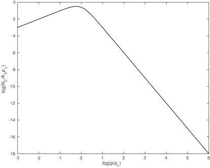
Figure 1.— Differential number density (87) of accelerated particles at the shock as a function of $p/p_{c}$ in the case $R=0$ for the adopted spectral index value $\rho=2$ and injection momentum $p_{0}/p_{c}=10^{-3}$.

In Fig. 1 we illustrate the Lorentzian differential number density of accelerated particles at the shock as a function of $p/p_{c}$. For particle momenta $p_{0}\leq p\leq p_{c}$ the Lorentzian distribution (87) increases linearly with momentum, $N_{0}(p_{0}\leq p\leq p_{c})\simeq A_{0}p$, whereas for large momenta $p\geq p_{c}$ it approaches the decreasing power law distribution

$$N_{0}(p\geq p_{c})\simeq A_{0}p_{c}\left({p\over p_{c}}\right)^{-\xi}$$ (90)

with

$$\xi=2\rho-1=1+{\psi\over 1+3\beta_{1}^{2}}$$

$$=1+{3\over(\Gamma_{1}\sqrt{r^{2}-\beta_{1}^{2}}-1)(1+3\beta_{1}^{2})}$$ (91)

Notice that for relativistic ($\Gamma_{1}\gg 1$) shock speeds the characteristic momentum (86) coincides with $mc$, so that in this case the no decreasing power law distributions for nonrelativistic shock accelerated particles result.

The Lorentzian distribution (87) attains its maximum value

$$N_{0,\rm max}=A_{0}p_{c}{(2\rho-1)^{\rho-{1\over 2}}\over(2\rho)^{\rho}}$$ (92)

at $p_{\rm max}=p_{c}/\sqrt{2\rho-1}$. The total number of accelerated particles at the shock is given by

$$N_{0,\rm tot}=\int_{p_{0}}^{\infty}N_{0}(p\geq p_{0})={A_{0}p_{c}^{2}\over 2(\rho-1)}\left[1+({p_{0}\over p_{c}})^{2}\right]^{1-\rho}$$

$$={4\pi S_{0}p_{0}^{2}\over U_{2}\Gamma_{2}}={4\pi S_{0}p_{0}^{2}\sqrt{r^{2}-\beta_{1}^{2}}\over c\beta_{1}}$$ (93)

The injection rate of charged particles in a partially ionized (with ionization fraction $\tau_{i}=n_{e1}/n_{\rm tot1}$) cold upstream medium is related to the upstream particle number flux $n_{\rm tot1}U_{1}$ as

$$S_{0}\delta(p-p_{0})={\tau_{i}\tau_{e}n_{\rm tot1}U_{1}\over p_{1}^{2}}\delta(p-p_{1})={\tau_{i}\tau_{e}n_{\rm tot1}c\beta_{1}\over p_{1}^{2}}\delta(p-p_{1}),$$ (94)

where the injection efficiency $\tau_{e}\ll 1$ indicates the small fraction of ionized upstream particles being accelerated. Then the total number of accelerated particles at the shock (93) is

$$N_{0,\rm tot}=4\pi\tau_{i}\tau_{I}n_{\rm tot1}\sqrt{r^{2}-\beta_{1}^{2}}$$ (95)

5.1. Nonrelativistic shock waves

For nonrelativistic shock velocities $\beta_{1}\ll 1$, so that $\Gamma_{1}\simeq 1$, Eq. (89) becomes

$$\rho\simeq{\psi_{0}\over 2}+1={2r+1\over 2(r-1)},$$ (96)

where we used

$$\psi_{0}={3\over r-1}$$ (97)

for the limit of Eq. (84) for $\beta_{1}\ll 1$. In this case the Lorentzian distribution function (87) reads

$$N_{0}(p\geq p_{0})=A_{0}p\left[1+({p\over\sqrt{3}\beta_{1}mc})^{2}\right]^{-{2r+1\over 2(r-1)}}$$ (98)

At momenta greater than the nonrelativistic characteristic momentum $p_{c}^{\rm nr}=\sqrt{3}\beta_{1}mc$ this function approaches the decreasing power law distribution

$$N_{0}(p\geq p_{c}^{\rm nr})\simeq A_{0}p_{c}^{\rm nr}\left({p\over p_{c}}\right)^{-\xi_{0}}$$ (99)

with the spectral index

$$\xi_{0}={r+2\over r-1}$$ (100)

This spectral index agrees with the standard result for nonrelativistic shocks providing $\xi_{0}\geq 2$ for shocks in adiabatic electron-proton media with compression ratios $r\leq 4$ and $\xi_{0}\geq 3/2$ for shocks in adiabatic electron-positron media with compression ratios $r\leq 7$.

5.2. Relativistic shock waves

For relativistic shock velocities with $\beta_{1}\simeq 1$ and $\Gamma_{1}\gg 1$, Eq. (89) becomes

$$\rho\simeq 1+{\psi\over 8}\simeq 1+{3\over 8(\Gamma_{1}\sqrt{r^{2}-1}-1)},$$ (101)

but now we have to distinguish between particle injection at nonrelativistic ($p_{0}\ll mc$) and at relativistic ($p_{0}\gg mc$) momenta.

In the first case the Lorentzian distribution function (87) reads

$$N_{0}(p\geq p_{0})=A_{0}p\left[1+({p\over mc})^{2}\right]^{-1-{3\over 8(\Gamma_{1}\sqrt{r^{2}-1}-1)}}$$ (102)

At nonrelativistic particle momenta this function increases linearly in momentum. At relativistic particle momenta it approaches the decreasing power law distribution

$$N_{0}(p\geq mc)\simeq A_{0}mc\left({p\over mc}\right)^{-\xi(\Gamma_{1}\gg 1)}$$ (103)

with the spectral index

$$\xi(\Gamma_{1}\gg 1)=1+{3\over 4(\Gamma_{1}\sqrt{r^{2}-1}-1},$$ (104)

which for $\Gamma_{1}\gg 1$ approaches unity. We defer the discussion of this spectral index to the next section where the acceleration of relativistic cosmic rays is investigated in more detail.

If cosmic rays are injected at relativistic momenta $p_{0}\gg mc$ the power law limit (90) of the distribution function (87) holds, so that with $p_{c}\simeq mc$ again Eq. (103) results. As $p_{0}\gg p_{c}$ the quantity (88) becomes

$$A_{0}={4\pi S_{0}\psi\over U_{2}\Gamma_{2}(1+3\beta_{1}^{2})}\left[{p_{0}\over mc}\right]^{2\rho},$$ (105)

providing for the distribution (103)

$$N_{0}(p\geq p_{0}\gg mc)\simeq{4\pi S_{0}\psi p_{0}\over U_{2}\Gamma_{2}(1+3\beta_{1}^{2})}\left({p\over p_{0}}\right)^{-\xi(\Gamma_{1}\gg 1)}$$ (106)

6. Relativistic cosmic rays

For relativistic particle momenta the integral (80) can be solved for general values of the helicity dependent function $R$. We assume here that cosmic ray particles are injected at relativistic momenta $p_{0}\gg mc$ with the monomomentum injection spectrum $S(p)=S_{0}\delta(p-p_{0})$. With $p\geq p_{0}\gg mc$ the integral (80) reduces to

$$I(p\geq p_{0}\gg mc)\simeq{1\over 1+\beta_{1}ZR+3\beta_{1}^{2}}\ln\left({p\over p_{0}}\right)$$ (107)

Consequently, the solution (81) becomes the power law distribution

$$N_{0}(p\geq p_{0}\gg mc)\simeq{4\pi S_{0}p_{0}\psi\over U_{2}\Gamma_{2}(1+\beta_{1}ZR+3\beta_{1}^{2})}\left({p\over p_{0}}\right)^{-\xi}$$ (108)

with the power law spectral index

$$\xi=1+{\psi\over 1+\beta_{1}ZR+3\beta_{1}^{2}}$$

$$=1+{3\over\left(\Gamma_{1}\sqrt{r^{2}-\beta_{1}^{2}}-1\right)\left(1+\beta_{1}ZR+3\beta_{1}^{2}\right)}$$ (109)

We first note that for $R=0$ the power law solution (108) agrees with the earlier derived expression (106) and that the spectral indices (109) and (91) agree.

6.1. Nonrelativistic shock waves

For nonrelativistic shock velocities $U_{1,2}\ll c$, so that $\Gamma_{1}\simeq 1+(\beta_{1}^{2}/2)$ and $\Gamma_{2}\simeq 1+(\beta_{1}^{2}/2r^{2})$, the particle power law spectral index (109) to first order in $\beta_{1}\ll 1$ reduces to

$$\xi=1+{3[1-ZR\beta_{1}]\over r-1}={r+2-3ZR\beta_{1}\over r-1}$$ (110)

To lowest order in $\beta_{1}$ we again reproduce the standard result for nonrelativistic shocks

$$\xi(\beta_{1}=0)={r+2\over r-1},$$ (111)

providing $\xi\geq 2$ for shocks in adiabatic electron-proton media with compression ratios $r\leq 4$ and $\xi\geq 3/2$ for shocks in adiabatic electron-positron media with compression ratios $r\leq 7$.

However, our result (110) gives a small (for turbulence spectral indices $s<2$) correction to this standard spectral index which is different for positively ($Z=1$) and negatively ($Z=-1$) charged cosmic ray particles. Depending on the sign of helicity dependent function $R$ defined Eq. (60) this implies either a smaller or greater spectral index compared to the standard result (111). With the maximum value (62) the correction is at most

$$|\Delta\xi|\leq{3R_{\rm max}\beta_{1}\over r-1}={6(2-s)(4-s)\over(3-s)(5-s)}{\beta_{1}\over r-1},$$ (112)

which for a Kolmogorov turbulence spectral index $s=5/3$ gives

$$|\Delta\xi|\leq{3R_{\rm max}\beta_{1}\over r-1}=1.05{\beta_{1}\over r-1},$$ (113)

For most adiabatic shocks with $r>1.1$ this is negligibly small as $|\Delta\xi|\leq 10.5\beta_{1}$.

6.2. Relativistic shock waves

The determination of the power law spectral indices (109) and (91) require the knowledge of the shock compression ratio $r=\beta_{1}/\beta_{2}$ which for relativistic shocks depends for any given shock speed $\beta_{1}$ in a non-trivial way on the equations of state of the up- and downstream fluids as shown for hyrodynamical shocks by Peacock (1981), Heavens and Drury (1988) and Kirk and Duffy (1999). The jump conditions for relativistic magnetohydrodynamic shocks in gyrotropic plasmas were studied by Double et al. (2004) and Gerbig and Schlickeiser (2011), including the pressure anisotropy $\chi=P_{\perp}/P_{\parallel}$ of the upstream and downstream gas pressures adopting adiabatic equation of states of the up- and down-stream gas with adiabatic indices $\kappa_{1,2}$. For a parallel ultrarelativistic shock ($\Gamma_{1}\gg 1$, $\beta_{1}\simeq 1$) Gerbig and Schlickeiser (2011) found the relations between the downstream parallel plasma beta $\beta_{\parallel 2}=8\pi P_{\parallel 2}/B_{0}^{2}$, the compression ratio $r=\beta_{1}/\beta_{2}$ and the anisotropies $\chi_{1,2}$.

For illustrating our results we consider here only the case of an ultrarelativistic shock $\Gamma_{1}\gg 1$ and a relativistic downstream medium with adiabatic index $4/3$, so that $\beta_{1}=3\beta_{2}$ (Blandford and McKee 1976) or $r=3$. In this case we obtain for the power law spectral indices (109) and (91)

$$\xi(\Gamma_{1}\gg 1)=1$$

$$+{3\over\left[\sqrt{8\Gamma_{1}^{2}+1}-1\right]\left[4-{3\over\Gamma_{1}^{2}}+ZR\sqrt{1-{1\over\Gamma_{1}^{2}}}\right]}$$

$$\simeq 1+{3\over 2\sqrt{2}[4+ZR]\Gamma_{1}}$$ (114)

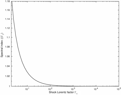
Figure 2.— Power law spectral index (114) of relativistic particles accelerated at an ultrarelativistic shock for the case $R=0$ as a function of the shock Lorentz factor $\Gamma_{1}$.

In Fig. 2 we calculate this spectral index for the case $R=0$ for relativistic shocks with $\Gamma_{1}\geq 2$, indicating spectral index values close to unity. Possible modifications and charge-sign dependencies (i.e. the case $R\neq 0$) will be considered elsewhere. Due to the dominating $\Gamma^{-1}$ dependence of $\xi-1$ the limit $\xi\simeq 1$ is reached for $\Gamma_{1}>10$.

Our result of flat spectral indices with $\xi\simeq 1$ for ultrarelativistic shock disagrees strongly with the earlier established universal spectral index value $\xi\in[2.25-2.30]$ from the eigenfunction and Monte Carlo simulation studies (for review see Kirk and Duffy 1999). As possible explanation for this difference we recall that our analytical solution is based on the two continuity conditions (57) and (58) at the shock. These two continuity conditions are needed as our steady-state diffusion-convection transport equation (54) is a second-order differential equation in the position coordinate $z$. While the continuity condition (57) for the particle phase density at the shock is also used in the eigenfunction solution method, the continuity condition (58) for the flux of particles is not used in that method as the Fokker-Planck transport equation (3) is a first-order differential equation in the position coordinate $z$. It is clear that the use of different continuity conditions results in different results.

7. Summary and conclusions

The analytical theory of diffusive cosmic ray acceleration at parallel stationary shock waves with magnetostatic turbulence is generalized to arbitrary shock speeds $V_{s}=\beta_{1}c$, including in particular relativistic speeds. This is achieved by applying the diffusion approximation to the relevant Fokker-Planck particle transport equation formulated in the mixed comoving coordinate system. In this coordinate system the particle’s momentum coordinates $p$ and $\mu=p_{\parallel}/p$ are taken in the rest frame of the streaming plasma, whereas the time and space coordinates are taken in the observer’s system. The Fokker-Planck particle transport equation contains connection coefficients resulting from the coordinate transformations into this mixed frame which are properly included in the diffusion approximation. For magnetostatic slab turbulence the diffusion-convection transport equation (45) for the isotropic (in the rest frame of the streaming plasma) part of the particle’s phase space density is derived for the first time for arbitrary shock speeds. In the limit of nonrelativistic flows the diffusion-convection transport equation differs from the transport equation used in earlier nonrelativistic diffusive shock acceleration theory (Axford et al. 1977, Krymsky 1987, Blandford and Ostriker 1978, Bell 1978, Drury 1983) by an additional term. This results from our correct handling of the connection coefficients. The additional term implies a velocity dependence of the acceleration rate and thus provides a major modification of the resulting differential momentum spectrum of accelerated particles in the nonrelativistic flow limit at nonrelativistic particles momenta: instead of a power law distribution of accelerated particles at the shock a Lorentzian distribution function results, which at large momenta then approaches the power law distribution inferred in earlier acceleration theories for nonrelativistic shock speeds.

For a step-wise shock velocity profile the steady-state diffusion-convection transport equation is solved analytically again for the first time for arbitrary shock speeds following closely the solution method developed for nonrelativistic speeds, making use of the continuity conditions (57) and (58) for the cosmic ray phase space density and streaming density at the shock. For a symmetric pitch-angle scattering Fokker-Planck coefficient $D_{\mu\mu}(-\mu)=D_{\mu\mu}(\mu)$ the steady-state solution is independent of the microphysical scattering details. For nonrelativistic mono-momentum particle injection at the shock the differential number density of accelerated particles is a Lorentzian-type distribution function which at large momenta approaches a power law distribution function $N(p\geq p_{c})\propto p^{-\xi}$ with the spectral index $\xi(\beta_{1})=1+[3/(\Gamma_{1}\sqrt{r^{2}-\beta_{1}^{2}}-1)(1+3\beta_{1}^{2})]$. For nonrelativistic ($\beta_{1}\ll 1$) shock speeds this spectral index agrees with the known result $\xi(\beta_{1}\ll 1)\simeq(r+2)/(r-1)$, whereas for ultrarelativistic ($\Gamma_{1}\gg 1$) shock speeds the spectral index value is close to unity. If particle injection occurs already at relativistic momenta, the steady-state solution is of power law type at all higher particle momenta.

For asymmetric pitch-angle scattering Fokker-Planck coefficient $D_{\mu\mu}(-\mu)\neq D_{\mu\mu}(\mu)$, resulting from magnetostatic isospectral slab Alfven waves with non-zero values of the magnetic and cross helicities, the momentum spectrum of accelerated particles depends on the microphysical details of particle’s pitch angle scattering. In particular, a dependence of the momentum spectrum on the charge sign of the cosmic ray particles is found. For turbulence spectral indices $s<2$, however, this difference is negligibly small. But steeper turbulence power spectra with $s\geq 2$ may provide stronger differences, which needs to be investigated in the future. Further future research topics will be concerned with the derivation of time-dependent solutions of the generalized diffusion-convection transport equation, the study of non-stationary flows, the inclusion of finite up- and downstream free escape boundary conditions, the investigation of the influence of finite frequency effects for low-frequency Alfven waves discarding the magnetostatic approximation, and the investigation of the influence of cosmic ray momentum losses. These additional effects have been studied before in great detail for nonrelativistic shocks, and it is of high interest to investigate their importance for relativistic shocks. The work presented here provides the analytical basis for these future studies.

8. Appendix A: the integral $I(p,p_{0})$

The integral (80) is be solved in closed form by

$$I(\beta,\beta_{0})=w(\beta)-w(\beta_{0}),\;\;\;w(x)={W_{1}(x)\over W_{2}},$$

$$W_{1}(x)=2(1-3\beta_{1}^{2})\arctan\left({ZR\beta_{1}+2x\over\beta_{1}\sqrt{12-R^{2}}}\right)$$

$$+\sqrt{12-R^{2}}\Bigl{[}\left(ZR\beta_{1}-1-3\beta_{1}^{2}\right)\ln(x-1)$$

$$-\left(1+3\beta_{1}^{2}+ZR\beta_{1}\right)\ln(1+x)$$

$$+\left(1+3\beta_{1}^{2}\right)\ln(3\beta_{1}^{2}+ZR\beta_{1}x+x^{2})\Bigr{]},$$

$$W_{2}=2\left[\left(1+3\beta_{1}^{2}\right)^{2}-R^{2}\beta_{1}^{2}\right)\sqrt{12-R^{2}}$$ (115)

References

• Batman (1940) Axford, W. I., Leer, E., Skadron, G., 1977,Proc. 15th Intern. Cosmic Ray Conf., Plovdiv, Bulgaria, Vol. 11, p. 132
• Batman (1940) Bell, A. R., 1978, MNRAS 182, 147
• Batman (1940) Bednarz, J., Ostrowski, M., 1998, PRL 80, 3911
• Batman (1940) Blandford, R., Eichler, D., 1987, Phys. Rep. 154, 1
• Batman (1940) Blandford, R., McKee, C. F., 1976, Phys. Fluids 19, 1130
• Batman (1940) Blandford, R., Ostriker, J. P., 1978, ApJ 221, L29
• Batman (1940) Double, G. P., Baring, M. G., Jones, F. C., Ellison, D. C., 2004, ApJ 600, 485
• Batman (1940) Drury, L. O. C., 1983, Rep. Progr. Phys. 46, 973
• Batman (1940) Dung, R., Schlickeiser, R. 1990, A& A 237, 504
• Batman (1940) Earl, J. A., 1974, ApJ 193, 231
• Batman (1940) Ellison, D. C., Jones, F. C., Reynolds, S. P., 1990, ApJ 360, 702
• Batman (1940) Gerbig, D., Schlickeiser, R., 2011, ApJ 733, 32
• Batman (1940) Hasselmann, K., Wibberenz, G., 1968, Z. Geophys. 34, 353
• Batman (1940) Heavens, A. F., Drury, L. O. C., 1988, MNRAS 235, 997
• Batman (1940) Hinton, J. A., Hofmann, W., 2009, ARAA 47, 523
• Batman (1940) Jokipii, J. R., 1976, ApJ 146, 480
• Batman (1940) Kirk,J. G., Duffy, P., 1999, J. Phys. G 25, R163
• Batman (1940) Kirk,J. G., Schneider, P., 1987, ApJ 315, 425
• Batman (1940) Kirk,J. G., Schneider, P., Schlickeiser, 1988, ApJ 328, 269
• Batman (1940) Kota, J., Merenyi, E., Jokipii, J. R., et al., 1982, ApJ 254, 398
• Batman (1940) Krymskii, G. F., 1077, Sov. Phys. Doklady 22, 327
• Batman (1940) Ostrowski, M., 1991, MNRAS 249, 551
• Batman (1940) Paczynski, B., 1998, ApJ 494, L45
• Batman (1940) Peacock, J. A., 1981, MNRAS 196, 135
• Batman (1940) Piran, T., 1999, Phys. Rep. 314, 575
• Batman (1940) Riffert, H., 1986, ApJ 310, 729
• Batman (1940) Roelof, E. C., 1969, in: Lectures in High Energy Astrophysics, eds. H. Ögelman and J. R. Wayland (NASA SP-199, Washington), p. 111
• Batman (1940) Schlickeiser, R., 2002, Cosmic Ray Astrophysics, Springer, Berlin
• Batman (1940) Schlickeiser, R., 2011, ApJ 732, 96
• Batman (1940) Shalchi, A., Nonlinear Cosmic Ray Diffusion Theories, Springer, Berlin
• Batman (1940) Sironi, L., Spitkovsky, A., 2009, ApJ 707, L92
• Batman (1940) Spitkovsky, A., 2008, ApJ 682, L5
• Batman (1940) Summerlin, E. J., Baring, M. G., 2012, ApJ 745, 63
• Batman (1940) Vietri, M., Stella, L., 1998, ApJ 507, L45
• Batman (1940) Webb, G. M., 1985, ApJ 296, 319
• Batman (1940) Woosley, S. E., 1993, ApJ 405, 273