Global coherence of quantum evolutions based on decoherent histories: theory and application to photosynthetic quantum energy transport

Abstract

Assessing the role of interference in natural and artificial quantum dyanamical processes is a crucial task in quantum information theory. To this aim, an appopriate formalism is provided by the decoherent histories framework. While this approach has been deeply explored from different theoretical perspectives, it still lacks of a comprehensive set of tools able to concisely quantify the amount of coherence developed by a given dynamics. In this paper we introduce and test different measures of the (average) coherence present in dissipative (Markovian) quantum evolutions, at various time scales and for different levels of environmentally induced decoherence. In order to show the effectiveness of the introduced tools, we apply them to a paradigmatic quantum process where the role of coherence is being hotly debated: exciton transport in photosynthetic complexes. To spot out the essential features that may determine the performance of the transport we focus on a relevant trimeric subunit of the FMO complex and we use a simplified (Haken-Strobl) model for the system-bath interaction. Our analysis illustrates how the high efficiency of environmentally assisted transport can be traced back to a quantum recoil avoiding effect on the exciton dynamics, that preserves and sustains the benefits of the initial fast quantum delocalization of the exciton over the network. Indeed, for intermediate levels of decoherence, the bath is seen to selectively kill the negative interference between different exciton pathways, while retaining the initial positive one. The concepts and tools here developed show how the decoherent histories approach can be used to quantify the relation between coherence and efficiency in quantum dynamical processes.

I Introduction

Coherence is ultimately the most distinctive feature of quantum systems. Finding a proper measure of the coherence present at different times scales in a quantum dynamical system is the first essential step for assessing the role of quantum interference in natural and artificial processes. This is of particular relevance for those quantum evolutions in which information or energy are transformed and transferred in order to achieve a given task with high efficiency. In this context the relevant questions are: how much and what kind of coherence is created vs destroyed by the dynamical evolution? How does coherence determine/enhance the performance of the given process? These are in general difficult questions and to be answered they require an appropriate and sufficiently comprehensive framework. A general and fundamental formalism to describe quantum interference is provided by the decoherent histories (DH) approach to quantum mechanics. DH have mainly found applications to foundational issues of quantum mechanics such as the formulation of a consistent framework to describe closed quantum systems, the emergence of classical mechanics from a quantum substrate, the solution of quantum paradoxes, decoherence theory, quantum probabilities Griffiths ; Griffiths-Book ; Omnes ; GMannHartle ; GellMannHartle ; ZurekHist ; Hartle_NegProb2008 ; GMann-Hartle_2014-1 . However, DH can also be a systematic tool for quantifying interference in quantum processes, and discussing its relevance therein. Indeed, DH provide a precise mathematical formalization of interference by means of the the so called decoherence matrix $\mathcal{D}$. The latter is built on the elementary notion of histories and allows one to describe the quantum features vs the classical ones in tems of interference between histories, or pathways if one resorts to the mental picture of the double slit experiments. It is however difficult to quantify in a compact and meaningful way the content of $\mathcal{D}$ and its implications for the dynamics of specific systems. Our first main goal is therefore to define and test appropriate measures allowing for the investigation of how interference can determine the performance of a given quantum information processing task. Starting from $\mathcal{D}$ and by its sub-blocks we define different functionals. In particular, we introduce a global measure of coherence $\mathcal{C}$ able to describe the coherence content of a general quantum evolution at its various time scales; an average (over different time-scales) measure of coherence; and average mesure of interference between histories leading to a specific output.

While the tools we introduce are of general interest and application, in order to test them we apply them to a specific but relevant instance of quantum dynamics taking place in photosynthetic membranes of bacteria and plants: quantum energy transport. Here the basic common mechanism is the following: a quantum excitation is first captured by the system and then migrates through a network of sites (chromophores) towards a target site, e.g., a reaction center, where the energy is transformed and used to trigger further chemical reactions. There is now an emerging consensus that efficient transport in natural and biologically-inspired artificial light-harvesting systems builds on a finely tuned balance of quantum coherence and decoherence caused by environmental noise Ishizaki-PCCP ; Ishizaki-PNAS ; Belcher-Virus ; Kevin-Bardeen_Original ; GiordaJCP , a phenomenon known as environment-assisted quantum transport (ENAQT). This paradigm has emerged with clarity in recent years, as modern spectroscopic techniques first suggested that exciton transport within photosynthetic complexes might be coherent over appreciable timescales Engel . Indeed, a growing number of experiments has provided solid evidence that coherent dynamics occurs even at room temperature for unusually long timescales (of the order of $100fs$) Collini ; Panit . Efforts to describe these systems have led to general models of ENAQT Kevin-Bardeen_Original ; Mohseni ; Mohseni2 ; Plenio ; Cao , depicting the complex interplay of three key factors: coherent motion, i.e., quantum delocalization of the excitation over different sites, environmental decoherence, and localization caused by a disordered energy landscape. So far, the presence of coherence in light-harvesting systems has been qualitatively associated to the observation of distinctive ‘quantum features’. Originally, coherence was identified with ‘quantum wavelike’ behavior as reflected by quantum beats in the dynamics of chromophore populations within a photosynthetic complex. Later works, employing quantum-information concepts and techniques, have switched attention towards quantum correlations between chromophores, in particular quantum entanglementCaruso ; Whaley ; GiordaLHCII ; Ishizaki . Besides being open to criticism (see, e.g., Miller ; Tiersch ), these approaches do not provide direct quantitative measures of coherence in the presence of noise. Therefore, in what follows, we shall apply the novel tools based on DH to a simple yet fundamental model of quantum energy transfer. We will focus on a relevant trimeric subunit of the Fenna-Matthews-Olson (FMO) complex, the first pigment-protein complex to be structurally characterized Blankenship . The trimer is virtually the simplest paradigmatic model retaining the basic charcteristics of a disordered transfer network and it can also be conceived as an essential building block of larger networks. For simplicity, we will use the well-known Haken-Strobl model Haken to describe the interplay between Hamiltonian and dephasing dynamics. While the model is an oversimplified description of the actual dynamics taking place in real systems, it allows to spot out the essential features that may determine the high efficiency of the transport. We shall initially focus on a new coherence measure $\mathcal{C}$, based on the decoherence matrix, and characterize its behavior verifying that it can consistently identify the bases and timescales over which quantum coherent phenomena are present during the evolution of the system. We shall then show how the average coherence exhibited on those time scales can be connected with the delocalization process. A more detailed analysis will be aimed at distinguishing between constructive and destructive interference affecting the histories ending at the site where the excitation exits the photosynthetic structure. By using the decoherence functional, we will show that the beneficial role of dephasing for the transport efficiency lies in a selective suppression of destructive interference, a fact that has been systematically suggested in the literature, but never expressed within a general and comprehensive framework that allows the quantitative evaluation of coherence and its effects.

The application of the introduced tools and methods based on DH to a simple yet paradigmatic system shows how one can properly quantify the coherence content of a complex quantum dynamics and elucidate the role of coherence in determining the overall efficiency of the process Pleniocoherence .

The paper is structured as follows. In Section II we review the basic decoherent histories formalism. In Section III we define the measure of coherence $\mathcal{C}$ and describe its meaning and properties. In Section IV we first introduce the used model for describing the energy transport in the selected trimeric complex. We then discuss the coherence properties of the excitonic transport: By means of the appropriate measures based on the decoherent histories formalism we identify the essential features that may determine the high efficiency of the transport. In Section V we briefly discuss how to extend our results to the whole FMO complex. In Section VI we summarize our results an draw our conclusions.

II Decoherent histories

The formalism of decoherent (or consistent) histories was developed in slightly different flavors by Griffiths Griffiths ; Griffiths-Book , Gell-Mann GMannHartle ; GMann-Hartle_2014-1 , HartleHartle_NegProb2008 and Omnès Omnes . DH provide a consistent formulation of quantum mechanics where probabilities of measurement outcomes are replaced by probabilities of histories. In this formulation, external measurement apparatuses are not needed, and then one does not need to postulate a “classical domain" of observers. As a consequence, quantum mechanics becomes a theory that allows the calculation of probabilities of sequences of events within any closed system, including the whole universe, without the necessity of invoking postulates about the role of measurement. In this framework, the “classical domain" can be seen to emerge as the description of the system becomes more and more coarse-grained.

The idea of ‘histories’ stems from Feynman’s ‘sum-over-histories’ formulation of quantum mechanics. As is known, any amplitude $\langle\psi_{f}|U(t_{f}-t_{0})|\psi_{i}\rangle$ between an initial and a final state can be expressed as a sum over paths, or histories: Upon inserting the identity decomposition $\mathbb{I}=\sum_{j}|j\rangle\langle j|=\sum_{j}P_{j}$ at differerent times $t_{1}\dots t_{N}$ we get

$$\langle\psi_{f}|U(t_{f}-t_{0})|\psi_{i}\rangle= \langle\psi_{f}|U(t_{f}-t_{N})\sum_{j_{N}}P_{j_{N}}U(t_{N}-t_{N-1})\dots$$

$$\dots U(t_{2}-t_{1})\sum_{j_{1}}P_{j_{1}}U(t_{1}-t_{0})|\psi_{i}\rangle=$$

$$=\sum_{j_{1\dots}j_{N}}\langle\psi_{f}|P_{j_{N}}(t_{N}) \dots P_{j_{1}}(t_{1})|\psi_{i}\rangle$$

where we use the Heisenberg notation $P_{j}(t)=U^{\dagger}(t-t_{0})P_{j}U(t-t_{0})$. Thus the total amplitude $\langle\psi_{f}|U(t_{f}-t_{0})|\psi_{i}\rangle$ is decomposed as a sum of amplitudes, each one corresponding to a different history identified by a sequence of projectors $P_{j_{N}}\dots P_{j_{1}}$.

The decoherent histories formalism assumes that histories are the fundamental objects of quantum theory and gives a prescription to attribute probabilities to (sets of) histories. A history is defined as a sequence of projectors at times $t_{1}<\dots<t_{N}$. Probabilites can be assigned within exhaustive sets of exclusive histories, i.e., sets of histories $\mathcal{S}_{N}=\{t_{1},\dots,t_{N},P_{j_{1}},\dots,P_{j_{N}}\}$ where subscripts $j_{1},\dots,j_{N}$ label different alternatives at times $t_{1},\dots,t_{N}$. Histories are exhaustive and exclusive in the sense that the projectors at each time satisfy relations of orthogonality $P_{j}P_{k}=\delta_{jk}P_{j}$, and completeness, $\sum_{j}P_{j}=\mathbb{I}$. In other words, the projectors $P_{j}$ define a projective measurement. Within a specified set, any history can be identified with the sequence of alternatives $\mathbf{j}\equiv j_{1},\dots,j_{N}$ realized at times $t_{1},\dots,t_{N}$.

Different alternative histories can be grouped together with a procedure called coarse-graining. Starting from histories $\mathbf{j}$ and $\mathbf{k}$ we can define a new, coarse-grained history $\mathbf{m}=\mathbf{j}\lor\mathbf{k}$ by summing projectors for all times $t_{\ell}$ such that $j_{\ell}$ and $k_{\ell}$ differ:

$$P_{m_{\ell}}=P_{j_{\ell}}+P_{k_{\ell}} \mbox{ if }j_{\ell}\neq k_{\ell}$$

$$P_{m_{\ell}}=P_{j_{\ell}} \mbox{ if }j_{\ell}=k_{\ell},$$

for all $\ell=1,\dots,N$. By iterating this procedure, one can obtain more and more coarse-grained histories. A special type of coarse-graining is the temporal coarse-graining: we group together histories $\mathbf{j},\mathbf{k},\dots,\mathbf{l}$ such that such that at some time $t_{\ell}$ we have $P_{j_{\ell}}+P_{k_{\ell}}+\dots P_{l_{\ell}}=\mathbb{I}$. Then the coarse-grained history $\mathbf{m}=\mathbf{j}\lor\mathbf{k}\lor\dots\lor\mathbf{l}$ contains only one-projector (equal to the identity) at time $t_{\ell}$, that can be neglected and hence removed from the string of projectors defining the history. On the other hand temporal fine-graining can be implemented for example by allowing different alternatives at a times $t_{k}\notin\{t_{1},..,t_{N}\}$. In particular, one can create new sets of histories $\mathcal{S}_{N+1}=\{t_{1},\dots,t_{N},t_{N+1},P_{j_{1}},\dots,P_{j_{N}},P_{j_{N+1}}\}$ from a given one $\mathcal{S}_{N}$ by adding different alternatives at time $t_{N+1}>t_{N}$; the sets $\mathcal{S}_{N+1}$ are fine grained versions of the sets $\mathcal{S}_{N}$.
Once we specify the initial state $\varrho$ and the (unitary) time evolution $U(t)$, we can assign any history $\mathbf{j}$ a weight

$$w_{\mathbf{j}}=\mbox{Tr}[C_{\mathbf{j}}\varrho C_{\mathbf{j}}^{\dagger}],\quad\mbox{with}\quad C_{\mathbf{j}}=P_{j_{N}}(t_{N})\dots P_{j_{1}}(t_{1})$$

where we use the Heisenberg notation $P_{j_{\ell}}(t_{\ell})=U(t_{\ell})P_{j_{\ell}}U(t_{\ell})^{\dagger}$. When the initial state is pure, $\varrho=|\psi_{i}\rangle\langle\psi_{i}|$ and the final projectors are one dimensional, $P_{j_{N}}=|\psi_{j_{N}}\rangle\langle\psi_{j_{N}}|$, this formula takes the simple form of a squared amplitude

$$w_{\mathbf{j}}=|\langle\psi_{j_{N}}|P_{j_{N-1}}(t_{N-1})\dots P_{j_{1}}(t_{1})|\psi_{i}\rangle|^{2}.$$ (1)

Weights cannot be interpreted as true probabilities, in general. Indeed, due to quantum interference between histories, the $w_{j}$ do not behave as classical probabilities. Indeed, consider two exclusive histories $\mathbf{j},\mathbf{k}\in\mathcal{S}$ and the relative coarse-grained history $\mathbf{m}=\mathbf{j}\lor\mathbf{k}$ by: $P_{m_{\ell}}=P_{j_{\ell}}+P_{k_{\ell}},\forall\ell$. If the $w_{\mathbf{j}}$ were real probabilities, we would expect $w_{\mathbf{m}}=w_{\mathbf{j}}+w_{\mathbf{k}}$. Instead, what we find is

$$w_{\mathbf{m}}=w_{\mathbf{j}}+w_{\mathbf{k}}+2Re(\mbox{Tr}[C_{\mathbf{j}}\varrho C_{\mathbf{k}}^{\dagger}]).$$

Due to the non-classical term $Re(\mbox{Tr}[C_{\mathbf{j}}\varrho C_{\mathbf{k}}^{\dagger}])$, representing quantum interference between the histories $\mathbf{j}$ and $\mathbf{k}$, the classical probability-sum-rule is violated. The matrix

$$\mathcal{D}_{\mathbf{j}\mathbf{k}}=\mbox{Tr}[C_{\mathbf{j}}\varrho C_{\mathbf{k}}^{\dagger}]=\mbox{Tr}[P_{j_{N}}U(t_{N}-t_{N-1})\dots P_{j_{1}}U(t_{1})\varrho U(t_{1})^{\dagger}P_{k_{1}}\dots U(t_{N}-t_{N-1})^{\dagger}P_{k_{N}}]$$ (2)

is called decoherence functional or decoherence matrix. The decoherence matrix can be thought of as a “density matrix over histories”: Its diagonal elements are the weights of histories and its off-diagonal elements are interferences between pairs of histories. The decoherence matrix has the following properties: i) it is Hermitian ii) it is semipositive definite iii) it is trace one iv) it is block-diagonal in the last index, $\mathcal{D}_{\mathbf{j}\mathbf{k}}=\delta_{j_{N}k_{N}}\mathcal{D}_{\mathbf{j}\mathbf{k}}$. Weights of coarse-grained histories can be obtained by summing matrix entries in an $n\times n$ block of the decoherence matrix corresponding to the original fine-grained histories. For istance, the weight of history $\mathbf{m}=\mathbf{j}\lor\mathbf{k}$ is obtained by summing entries of a $2\times 2$ block of the decoherence matrix:

$$w_{\mathbf{m}}=\mathcal{D}_{\mathbf{j}\mathbf{j}}+\mathcal{D}_{\mathbf{k}\mathbf{k}}+\mathcal{D}_{\mathbf{j}\mathbf{k}}+\mathcal{D}_{\mathbf{k}\mathbf{j}}.$$

A necessary and sufficient condition to guarantee that the probability sum rule $w_{\mathbf{j}\lor\mathbf{k}}=w_{\mathbf{j}}+w_{\mathbf{k}}$ apply within a set of histories is

$$Re[\mathcal{D}_{\mathbf{j}\mathbf{k}}]=0,\forall\mathbf{j}\neq\mathbf{k}.$$

This condition is termed as weak decoherenceGellMannHartle ; the necessary and sufficient condition that is typically satisfied GellMannHartle and that we will adopt in the following is the stronger one termed as medium decoherence

$$\mathcal{D}_{\mathbf{j}\mathbf{k}}=0,\forall\mathbf{j}\neq\mathbf{k}.$$ (3)

Medium decoherence implies weak decoherence. Any exhaustive and set of exclusive histories satisfying medium decoherence is called a decoherent set. The fundamental rule of DH approach is that probabilities can be assigned within a decoherent set, each history being assigned a probabability equal to its weight. If medium decoherence holds, the diagonal elements of the decoherence matrix can be identified as real probabilities for histories and we can write $\mathcal{D}_{\mathbf{j}\mathbf{j}}=p_{\mathbf{j}}$.

Due to property iv), if we perform a temporal coarse-graining over all times except the last, we obtain ‘histories’ with only one projection, $P_{j_{N}}$ at the final time $t_{N}$. These histories automatically satisfy medium decoherence:

$$\sum_{j_{1},\dots,j_{N-1}}\sum_{k_{1},\dots k_{N-1}}\mathcal{D}_{\mathbf{j}\mathbf{k}} =$$

$$=\delta_{j_{N}k_{N}}\mbox{Tr}[P_{j_{N}}(t_{N})\varrho P_{j_{N}}(t_{N})] \equiv\delta_{j_{N}k_{N}}p_{j_{N}}$$

where $p_{j_{N}}\equiv\mbox{Tr}[P_{j_{N}}(t_{N})\varrho P_{j_{N}}(t_{N})]$ is the probability that the system is in $j_{N}$ at time $t_{N}$. Due to interference, the probability of being in $j_{N}$ at time $t_{N}$ is not simply the sum of probabilities of all alternative paths leading to $j_{N}$, i.e, of all alternative histories with final projection $P_{j_{N}}$. In formulas,

$$p_{j_{N}}\neq\sum_{j_{1},\dots j_{N-1}}w_{\mathbf{j}}=\sum_{j_{1},\dots j_{N-1}}\mathcal{D}_{\mathbf{j}\mathbf{j}}.$$

The probability and the global interference of histories $\mathcal{I}_{j_{N}}(\tau)$ ending in $j_{N}$ can be thus expressed as

$$p_{j_{N}}(\tau)=\sum_{j_{1},\dots j_{N-1}}w_{\mathbf{j}}(\tau)+\mathcal{I}_{j_{N}}(\tau)$$ (4)

with $\tau=N\Delta t\,$. Destructive interference will happen when $\mathcal{I}_{j_{N}}<0$, constructive interference when $\mathcal{I}_{j_{N}}>0$.

The decoherent histories formalism is consistent with and encompasses the model of environmentally induced decoherenceZurekHist . Given a factorization of the Hilbert space into a subsystem of interest and the rest (environment), $\mathcal{H}=\mathcal{H}_{S}\otimes\mathcal{H}_{\mathcal{E}}$, the events of a history take the form $P_{j_{\ell}{j^{\prime}}_{\ell}}=\tilde{P}_{j_{\ell}}\otimes\Pi_{{j^{\prime}}_{\ell}}$ where $\tilde{P}_{j_{\ell}}$ and $\Pi_{j^{\prime}_{\ell}}$ are projectors onto Hilbert subspaces of $\mathcal{H}_{S}$ and $\mathcal{H}_{\mathcal{E}}$ respectively. Histories for $S$ alone can be obtained upon considering appropriate coarse-grainings over the degrees of freedom of the environment, such that the events are $\tilde{P}_{j_{\ell}}\otimes\mathbb{I}_{\mathcal{E}}$ where $\mathbb{I}_{\mathcal{E}}$ is the identity over $\mathcal{H}_{\mathcal{E}}$. Upon introducing the time-evolution propagator $\mathcal{K}_{t\ t_{0}}$ as $\varrho(t)=U(t-t_{0})\varrho(t_{0})U(t-t_{0})^{\dagger}\equiv\mathcal{K}_{t\,t_{0}}[\varrho(t_{0})]$, we can rewrite the decoherence matrix as:

$$\mathcal{D}_{\mathbf{j}\mathbf{k}}= \mbox{Tr}[\tilde{P}_{j_{N}}\mathcal{K}_{t_{N}\ t_{N-1}}[\tilde{P}_{j_{N-1}}\mathcal{K}_{t_{N-1}\ t_{N-2}}[$$ (5)

$$\dots\mathcal{K}_{t_{1}\ t_{0}}[\varrho_{0}]\dots]\tilde{P}_{k_{N-1}}]\tilde{P}_{k_{N}}].$$

If the initial state is factorized $\varrho(t_{0})=\tilde{\varrho}_{S}(t_{0})\otimes\varrho_{\mathcal{E}}(t_{0})$, then the reduced density matrix $\varrho_{S}(t)=Tr_{\mathcal{E}}[\varrho(t)]$ evolves according to $\varrho_{S}(t)=\tilde{\mathcal{K}}_{t\ t_{0}}\varrho_{S}(t_{0})$ where $\tilde{\mathcal{K}}$ is the (non-unitary) reduced propagator defined by

$$\small\mbox{Tr}_{\mathcal{E}}[U(t-t_{0})\tilde{\varrho_{S}}(t_{0})\otimes\varrho_{\mathcal{E}}(t_{0})U^{\dagger}(t-t_{0})]=\tilde{\mathcal{K}}_{t\ t_{0}}[\tilde{\varrho}_{S}(t_{0})].$$ (6)

If the evolution of the system and environment is Markovian, we can write $\tilde{\mathcal{K}}_{t\ t^{\prime}}=\tilde{\mathcal{K}}_{t-t^{\prime}}$. As proved by Zurek ZurekHist , under the assumption of Markovianity we can rewrite the decoherence matrix in terms of reduced quantities alone, i.e., quantities pertaining to the system only:

$$\mathcal{D}_{\mathbf{j}\mathbf{k}}= \mbox{Tr}_{S}[\tilde{P}_{j_{N}}\tilde{\mathcal{K}}_{t_{N}\ t_{N-1}}[\tilde{P}_{j_{N-1}}\tilde{\mathcal{K}}_{t_{N-1}\ t_{N-2}}[\dots\tilde{\mathcal{K}}_{t_{1}\ t_{0}}[\varrho_{0}]\dots]\tilde{P}_{k_{N-1}}]\tilde{P}_{k_{N}}].$$ (7)

That is, the model of environmentally induced decoherence can be obtained by applying the decoherent histories formalism to system and environment together, and by coarse-graining over the degrees of freedom of the environment.

III The coherence measure $C$

The DH approach provides the most fundamental framework in which the transition from the quantum to the classical realm can be expressed. Indeed, it is based on the most basic feature characterizing the quantum world: interference and the resulting coherence of the dynamical evolution. Despite being a well developed field of study, the DH history approach lacks for a proper global measure of the coherence produced by the dynamics at the different time scales. We therefore introduce a measure that quantifies the global amount of coherence within a set of histories. Assume projectors for all times $t_{\ell},\ell=1,\dots,N$ are taken in a fixed basis $|e_{j}\rangle$, $P_{j}^{\ell}=|e_{j}\rangle\langle e_{j}|$. Assume further that histories are composed by taking equally spaced times between consecutive projections i.e., $t_{1}=\Delta t,\dots,t_{N}=N\Delta t$. (in other words, histories correspond to projections applied in the same basis and repeated at regular times). For such a set of histories, consider the decoherence matrix

$$\mathcal{D}_{\mathbf{j}\mathbf{k}}^{(N,P,\Delta t)}=\mbox{Tr}[C_{\mathbf{j}}^{(N,P,\Delta t)}\varrho C_{\mathbf{k}}^{(N,P,\Delta t)}]$$

where $C_{\mathbf{j}}^{(N,P,\Delta t)}=P_{j_{N}}(N\Delta t)\dots P_{j_{1}}(\Delta t)$. Take the von Neumann entropy of the decoherence matrix,

$$h(P,N,\Delta t)=-\mbox{Tr}[\mathcal{D}^{(N,P,\Delta t)}\log\mathcal{D}^{(N,P,\Delta t)}].$$ (8)

Due to coherence between histories, $h_{N}$ differs from the ‘classical-like’ Shannon entropy of history weights

$$h^{(c)}(P,N,\Delta t)=-\sum_{\mathbf{j}}w_{\mathbf{j}}^{(N,P,\Delta t)}\log w_{\mathbf{j}}^{(N,P,\Delta t)}$$ (9)

where $w_{\mathbf{j}}^{(N,P,\Delta t)}=\mbox{Tr}[C_{\mathbf{j}}^{(N,P,\Delta t)}\varrho C_{\mathbf{j}}^{(N,P,\Delta t)}]$ are the diagonal elements of $\mathcal{D}^{(N,P,\Delta t)}$, i.e., the weights. The difference between the two quantities is wider if off-diagonal elements of the decoherence matrix are bigger, i.e., if the set of histories is more coherent. Let us define:

$$C(P,N,\Delta t)\equiv\frac{h^{(c)}(P,N,\Delta t)-h(P,N,\Delta t)}{h^{(c)}(P,N,\Delta t)}.$$ (10)

We argue that $C(P,N,\Delta t)$ is suitable to be used as a general measure of coherence within the set of histories defined by $P,N,\Delta t$. Indeed, we can readily prove the following properties:
i) $0\leq C(P,N,\Delta t)<1$. $C(P,N,\Delta t)<1$ is obvious. To prove $C(P,N,\Delta t)>0$, let us define a matrix $\tilde{\mathcal{D}}_{\mathbf{j}\mathbf{k}}^{(N,P,\Delta t)}=\delta_{\mathbf{j}\mathbf{k}}\mathcal{D}_{\mathbf{j}\mathbf{k}}^{(N,P,\Delta t)}$ where off-diagonal entries are set to zero. Since

$$\mbox{Tr}[\mathcal{D}^{(N)}\log\tilde{\mathcal{D}}^{(N)}] =\sum_{\mathbf{j}}D_{\mathbf{j},\mathbf{j}}^{(N,P,\Delta t)}\log D_{\mathbf{j},\mathbf{j}}^{(N,P,\Delta t)}=$$

$$=\mbox{Tr}[\tilde{\mathcal{D}}^{(N,P,\Delta t)}\log\tilde{\mathcal{D}}^{(N,P,\Delta t)}]$$

we obtain that the numerator of (10) can be expressed as a quantum relative entropy:

$$\ h^{(c)}(P,N,\Delta t)-h(P,N,\Delta t)=$$

$$-\mbox{Tr}[\tilde{\mathcal{D}}^{(N,P,\Delta t)}\log\tilde{\mathcal{D}}^{(N,P,\Delta t)}]+\mbox{Tr}[\mathcal{D}^{(N,P,\Delta t)}\log\mathcal{D}^{(N,P,\Delta t)}]$$

$$=\mbox{Tr}[\tilde{\mathcal{D}}^{(N,P,\Delta t)}(\log\mathcal{D}^{(N,P,\Delta t)}-\log\tilde{\mathcal{D}}^{(N,P,\Delta t)})]$$

$$=h(\mathcal{D}^{(N,P,\Delta t)}||\tilde{\mathcal{D}}^{(N,P,\Delta t)})\geq 0$$

where $h(A||B)\geq 0$ is the relative entropy between $A$ and $B$.
ii) $C(P,N,\Delta t)=0$ iff $\mathcal{D}_{\mathbf{j},\mathbf{j}}^{(N,P,\Delta t)}=\tilde{\mathcal{D}}_{\mathbf{j},\mathbf{j}}^{(N,P,\Delta t)}$, i.e., $C(P,N,\Delta t)$ vanishes if medium decoherence holds for the set of histories, since the two quantities $h(N,P,\Delta t)$ and $h^{(c)}(N,P,\Delta t)$ coincide in this case.

Thus $C(P,N,\Delta t)$ is in essence a (statistical) distance between the decoherence matrix $\mathcal{D}$ and the corresponding diagonal matrix $\tilde{\mathcal{D}}^{(P,N,\Delta t)}$, renormalized so that its value lies between $0$ and $1$. The greater are the off-diagonal elements of $\mathcal{D}^{(P,N,\Delta t)}$, the greater the distance. The meaning of $C(P,N,\Delta t)$ can be easily understood if we use the linear entropy, a lower bound to the logarithmic version:

$$h_{L}(P,N,\Delta t)=1-\mbox{Tr}[(\mathcal{D}^{(N,P,\Delta t)})^{2}],$$

$$1-h_{L}^{(c)}(P,N,\Delta t)=\mbox{Tr}[(\tilde{\mathcal{D}}^{(N,P,\Delta t)})^{2}].$$

In this case, we obtain a ‘linear entropy’ proxy of $C(N,P,\Delta t)$ as:

$$C_{L}(P,N,\Delta t)\equiv\frac{h_{L}^{(c)}(P,N,\Delta t)-h_{L}(P,N,\Delta t)}{h_{L}^{(c)}(P,N,\Delta t)}=$$

$$=\frac{\sum_{\mathbf{j}\neq\mathbf{k}}|\mathcal{D}_{\mathbf{j}\mathbf{k}}^{(N,P,\Delta t)})|^{2}}{1-\sum_{\mathbf{j}}|\mathcal{D}_{\mathbf{j}\mathbf{j}}^{(N,P,\Delta t)})|^{2}}$$

which is a simplified version that, by avoiding the diagonalization of $\mathcal{D}^{(N,P,\Delta t)}$, helps containing the numerical complexity.

The measure introduced is well grounded on physical considerations. In the following we will apply it to a simple system in order to check its consistency, and later use it to characterize the coherence properties of the evolutions induced by various regimes of interaction with the environment. First, one has to check whether the measure properly takes into account the action of the bath. In particular, if the bath is characterized by a decoherence time $\gamma^{-1}$, it is known (ZurekHist ) that on time scales $\Delta t\geq\gamma^{-1}$ the decoherence matrix becomes diagonal: The probability of a history at time $t_{N+1}$ can be fully determined by its probability at time $t_{N}$, since no interference can occur between different histories. Indeed, the action of the bath is to create a decoherent set of histories that are defined by a proper projection basis: the pointer basis (ZurekHist ). Therefore, the fine-graining procedure obtained by constructing a set of histories $\mathcal{S}_{N+1}$ via the addition of a new complete set of projections in the same basis at time $t_{N+1}=(N+1)\Delta t$ to the set $\mathcal{S}_{N}$, should leave the coherence functional $C$ invariant, i.e., $C(P,N+1,\Delta t)\approx C(P,N,\Delta t)$. If instead $\Delta t<\gamma^{-1}$ the same fine-graining procedure should lead to $C(P,N+1,\Delta t)\geq C(P,N,\Delta t)$.

Before passing to analyze a specific system, we want to focus on the complexity of the evaluation of $\mathcal{D}$ and $\mathcal{{C}}$. The dimension of the decoherent matrix grows with the dimension $d$ of the basis $P$ and the number $N$ of time instants that define each history as $d^{2N}$. This exponential growth in principle limits the application of the DH approach to small systems. However, as for the system considered in this paper the computational effort is contained due to the small number of subsystems (chromophores) and the small dimension of the Hilbert space which is limited to the single-exciton manifold. As we shall see, by limiting the choice of $N$ to a reasonable number, the analysis can be fruitfully carried even on a laptop.

IV Trimer

We now start to analyze decoherent histories in simple models of energy transfer comprising a small number $d$ of chromophores (sites). Neglecting higher excitations, each site $i$ can be in its ground $|0\rangle_{i}$ or excited $|1\rangle_{i}$ state. We work in the single-excitation manifold, and define the site basis as

$$|i\rangle\equiv|0\rangle_{1}\dots|1\rangle_{i}\dots|0\rangle_{d}\qquad i=1\dots d,$$

i.e., state $|i\rangle$ represents the exciton localized at site $i$. On-site energies and couplings are represented by a Hamiltonian $H$ that is responsible for the unitary part of the dynamics. Interaction with the environment is implemented by the Haken-Strobl model, that has been extensively used in models of ENAQT Mohseni ; Plenio ; GiordaLHCII ; Cao . The effect of the environment is represented by a Markovian dephasing in the site basis, expressed by Lindblad terms $L$ in the evolution, as follows:

$$\dot{\varrho}=[H,\varrho]+\sum_{i}\gamma_{i}[2L_{i}\varrho L_{i}^{{\dagger}}-L_{i}^{{\dagger}}L_{i}\varrho-\varrho L_{i}^{{\dagger}}L_{i}]$$ (11)

where $L_{i}=|i\rangle\langle i|$ are projectors onto the site basis, and $\gamma_{i}$ are the (local) dephasing rates. Furthermore, site $d$ can be incoherently coupled to an exciton sink, represented by a Linblad term

$$k_{trap}[2L_{trap}\varrho L_{trap}^{{\dagger}}-L_{trap}^{{\dagger}}L_{trap}\varrho-\varrho L_{trap}^{{\dagger}}L_{trap}]$$

where $L_{trap}=|sink\rangle\langle e|$ and $k_{trap}$ is the trapping rate. Contrary to other works, we neglect exciton recombination, as it acts on much longer timescales $(\sim 1\>ns)$ than dephasing and trapping.
The global evolution is Markovian and can be represented by means of the Liouville equation

$$\dot{\varrho}=\mathcal{L}(\varrho)=\mathcal{L}_{H}(\varrho)+\mathcal{L}_{\gamma}(\varrho)+\mathcal{L}_{{trap}}(\varrho)$$ (12)

that can be simply solved by exponentiation,

$$\varrho(t)=e^{i\mathcal{L}t}(\varrho(0)).$$ (13)

In the notation above, the propagator has the form $\tilde{\mathcal{K}}_{t^{\prime}t}=e^{i\mathcal{L}(t^{\prime}-t)}$. The efficiency of the transport can be evaluated as the leak of the population $p_{e}(t)=\langle e|\rho|e\rangle$ of the exit site $e$ towards the sink:

$$\eta(t)=2k_{trap}\intop_{0}^{t}\langle e|\rho|e\rangle.$$ (14)

The overall efficiency of the process is obtained by letting $t\rightarrow\infty.$

While its Markovianity limits the faithful description of decoherence processes actually taking place in real photosynthetic systems, the model retains the basic and commonly accepted aspects of decoherence, that acts in the site basis: albeit in a complex non-Markovian way, the protein enviroment measures the system locally (i.e., on each site), thus destroying the coherence in the site basis and creating it in the exciton basis. Note that the formalism can also be applied to a ‘dressed’ or polaronic basis where we include strong interactions between chromophores and vibrational modes. That is, to apply the DH method, one only needs a model in which an exciton hops between sites, dressed or undressed. The model is therefore suitable to readily implement the decoherent histories paradigm and to spot the main basic features we are interested in and that are at the basis of the success of ENAQT.

The FMO unit has $7$ chromophores and a complex energy and coupling landscape with no symmetries. Energies and couplings (i.e., the Hamiltonian $H$) can be obtained by different techniques: They can be extracted by means of 2D spectroscopy as in Cho or computed through ab initio calculations as in Renger , with similar but not exactly equal results. This very complex struxture makes FMO far from ideal as a first example to study. We thus prefer to start by working with a much simpler, yet fully relevant subsystem: the trimeric unit composed by the sites $1,2$ and $3$ of the FMO complex in the notation of Renger ; Cho ). The first chromophore is the site in which the energy transfer begins, while the third chromophore is the site from which the excitation leaves the complex. The Hamiltonian of the trimeric subunit is Renger

$$H_{Renger}=\left(\begin{array}[]{ccc}215&-104.1&5.1\\ -104.1&220&32.6\\ 5.1&32.6&0\end{array}\right).$$ (15)

The eigenenergies of the system ar given by $E_{+}=322.85\,cm^{-1},$$E_{-}=119.13\,cm^{-1},$ $\,E_{3}=-6.98\,cm^{-1}$ which yields the eigenperiods $T_{ij}=(2\pi\hbar/\Delta E_{ij}):$ $T_{+-}=0.163\,ps,\,T_{-3}=0.100\,ps,\,T_{+3}=0.264\,ps$. Due its structure, the trimer is a chain composed by a pair of chromophores ($1,2$), degenerate in energy and forming a strongly coupled dimer, and a third chromophore moderately coupled with the second one only. Since in the following we suppose that the exciton starts from site $1$, we expect a prominent role of the dimer in the dynamics, at least in the first tens of femtoseconds.

In order to show how the DH analysis can be implemented, in the following we are going to consider histories in the site and the energy bases, with $N$ projections at times $n\Delta t,\>n=1,..,N$. We first use the coherence function $C(P,N,\Delta t)$ introduced above (10) to evaluate the global coherence of the exciton transport process. In order to test the behavior of $C$ for different values of dephasing, in Fig 1 we first plot $C$ as a function of the time interval $\Delta t$ between projections for two values of the dephasing rate: $i)\,\gamma=0$, corresponding to the full quantum regime (Fig.1) for the site basis (a); $ii)\>\gamma=10$ corresponding to an intermediate value of dephasing (Fig. 1) for the site basis (b) and the energy basis (c).

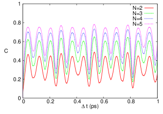
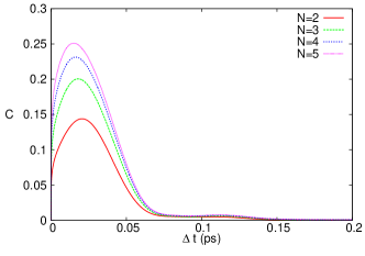
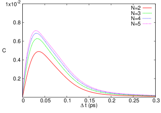
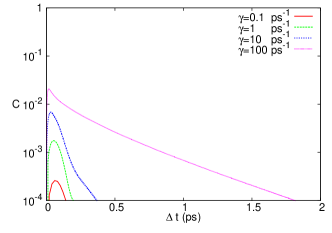
Figure 1: Coherence function $C(P,N,\Delta t)$ as a function of $\Delta t$ for the trimer with Hamiltonian 15 evaluated: (a) in the site basis for $\gamma=0$, (b) in the site basis for $\gamma=10ps^{-1}$ (c) in the exciton basis for $\gamma=10ps^{-1}$ (d) in the exciton basis for different values of dephasing $\gamma$.

Before entering the discussion of the various regimes, we note that as a function of the number of projections $N$ all curves display the expected behavior: The increase (decrease) of the number of projections corresponds to a temporal fine-graining (coarse-graining) of the evolution; therefore, an increase (decrease) of $N$ should imply an increase (decrease) of the amount of coherence between histories. As shown in Fig. (1) the function $C$ correctly reproduces the fine (coarse) graining feature: the qualitative behavior of $C$ as a function of $\Delta t$ is not affected by the choice of $N$, while an increase of $N$ corresponds, at fixed $\Delta t$, to an increase of $C$. We will therefore use in the following the value $N=4$ that allows for a neat description of the phenomena and for a reasonable computational time.

As for the behavior at fixed $N$, we have that in the full quantum regime ($\gamma=0$), the system obviously displays coherence in the site basis only since

$$\mbox{Tr}[|E_{i}\rangle\langle E_{i}|e^{-iH\Delta t}\rho e^{iH\Delta t}|E_{j}\rangle\langle E_{j}|]=\langle E_{i}|\rho|E_{i}\rangle\delta_{i,j}$$

and the decoherence matrix $\mathcal{D}$ in the energy basis is diagonal and independent on $\Delta t$ and $N$. This simply means that in the full quantum regime histories in the exciton basis are fully decohered, since the system is not able to create coherence among excitons. Still in the full quantum regime, in the site basis, the coherence oscillates as the exciton, starting at site $1$, goes back an forth along the trimer, and the evolution builds up coherence in this basis, see Fig.1 (a). In this regime, the trimer can be approximately seen as a dimer composed by the first two chromophores, and the exciton performs Rabi oscillations with a period given by $T_{+-}=160\,fs$; $C$ oscillates with half the period: for $\Delta t=80\,fs$ the exciton is migrated mostly on site $2$ and $C$ has a minumum – which is different from zero since the exciton is partly delocalized on site $3$, and the system therefore exhibits a non vanishing coherence.

For intermediate values of $\gamma\approx 10\,ps^{-1}$ , Fig.1 (b), the coherence in site basis as measured by $C$ correctly drops down at $\Delta t\geq\gamma^{-1}$ZurekHist . The dephasing has a strong and obvious effect on the coherence between pathways: coherence in this basis is a monotonically decreasing function of $\gamma$. This is well highlighted by the global coherence function $C$, whose maximal values are reduced by a factor of $\sim 3$ with respect to those corresponding to full quantum regime. After a time $\tau_{decoh}=\gamma^{-1}$ the histories are fully decohered. Indeed, due to the specific model of decoherence (11), which amounts to projective measurements on $|i\rangle\langle i|$ at each site with a rate $\gamma$, the system kills the coherence in the site basis, which in turn corresponds to the stable pointer basis for this model ZurekHist , i.e., the basis in which the density matrix is forced to be diagonal by the specific decoherence model. On the other hand, and for the same reason, the dynamics starts to build up coherence in the exciton basis $|E_{i}\rangle\langle E_{i}|$, see Fig. 1(c). However, this coherence is later destroyed - on a time scale of approximately $0.2\>ps$ - since the stationary state of the model is the identity. This effect is even more evident if one compares the behavior of $C$ in the exciton basis for different values of $\gamma$, as shown in Fig. 1(d): $C$ grows with $\gamma$ and it lasts over longer time scales. This feature is coherent with the expectations: the equilibrium state for high $\gamma$ is the identity. Due to the projections implemented by the environment in the site basis, the system is forced to create coherence in the exciton basis. When $\gamma$ is very high a quantum Zeno effect takes in, the dynamics is blocked, and the time required to reach the equilibrium, and to destroy coherences in all bases, consequently grows.

This first analysis therefore shows that $C$ is indeed a good candidate for assessing the global coherence properties of quantum evolutions. For a fixed number of projections $N$, $C(\Delta t)$ can be interpreted as a measure of the global coherence exhibited by the dynamics over the time scale $\Delta t$.

We now analyze in detail the specific features of quantum transport for the trimer. The dynamics starts at site $1$ and evolves by delocalizing the exciton on the other chromophores. In order to study this process, we first use a measure of delocalization introduced inGiordaLHCII for the study of LHCII complex dynamics:

$$\mathcal{{H}}(t)=-\sum_{i}p_{i}(t)\ln p_{i}(t)$$ (16)

that is simply the Shannon entropy of $p_{i}(t)$, the populations of the three chromophores. This measure allows one to follow how much the exciton gets delocalized over the trimer with time and in different dephasing situations: $0\leq\mathcal{{H}}(t)\leq\ln(3)$, i.e., $\mathcal{{H}}$ is zero when the exciton is localized on a chromophore and it takes its maximal value $\ln(3)$ when the population of the three sites are equal. In Fig. 2 we plot both $\mathcal{{H}}(t)$ and the population $p_{3}(t)$ of site $3$ for different values of $\gamma$. Due to the presence of interference, in the mainly quantum regime ($\gamma=0.1,1\>ps^{-1}$), the exiton first delocalizes mainly over the dimer and partly on the third site: The first maximum corresponds to $t=40\>fs=1/4\ T_{+-}$ when the system builds up a (close to uniform) coherent superposition between sites $1$ and $2$, while a non negligible part of the exciton is found in site $3$; indeed $\mathcal{{H}}(t=40\,fs)\approx 0.75>0.69$, the last value corresponding to $\ln(2)$ i.e., to a uniform superposition over the sites $1$ and $2$ only. As the dynamics of the sytems extends to later times we see that $\mathcal{{H}}(t)$ and $p_{3}(t)$ have an oscillatory behavior, whose main period is $1/2\ T_{+-}$, and which approximately corresponds to Rabi oscillations between site $1$ and $2$, although the initial state fully localized in site $1$ cannot be rebuilt due to the presence of site $3$. As for the transport, we see that in this regime the system cannot take advantage of the initial fast and high delocalization: the exciton bounces back and forth over the trimer. In the intermediate regime $\gamma=16\>ps^{-1}$, due, as we will later see, to the selective suppression of interference processes, the initial speed up in delocalization is sustained by the dynamical evolution, and the transfer rate to site $3$ is correspondingly increased. For very high values of decoherence ($\gamma=100$) the role of initial interference is suppressed and the initial speed-up disappears: the environment measures the system in site basis at high rates and the delocalization process is highly reduced.

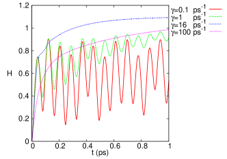
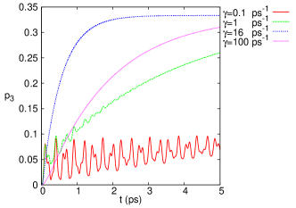
Figure 2: For the trimer (15): (a) Delocalization $\mathcal{{H}}(t)$ and (b) $p_{3}(t)$ population of site $3$ as a function of time for different values of $\gamma=0.1,1,16,100$ $ps^{-1}$

The optimal delocalization occurs in correspondence of $\gamma\approx 16\>ps^{-1}$ and it can be interpolated with a double exponential function

$$\mathcal{{H}}_{\gamma=16}(t)=c_{0}+c_{1}e^{-t/\tau_{1}}+c_{2}e^{-t/\tau_{2}}$$

with $c_{0}=1.098=\ln 3,\,c_{1}=-0.84,\,c_{2}=-0.373$. The first time scale $\tau_{1}=23\>fs$ describes the initial fast quantum delocalization process described above, while the second time scale $\tau_{2}=238\>fs$ the slower subsequent delocalization and the reaching of the equilibrium situation, $\mathcal{{H}}(t=\infty)=\ln(3)$.

We now pass to systematically analyze the behavior of the coherence of the evolution with respect to the strength of the interaction with the environment and its relevance for the energy transport process. As a first step we plot both $\mathcal{{H}}(\tau=N\Delta t)$ and $\mathcal{{C}}(\Delta t)$ for different values of $\gamma$, Fig. (3). The plots show that the coherence function exhibits the required behavior: For small $\gamma=0.1$ , $\mathcal{{C}}(\Delta t)$ oscillates with period $1/2\ T_{+-}$, following the Rabi oscillations of the dimer. The minima occur at $n/4\ T_{+-}$ , showing that the exciton is “partially” localized on site $1$ or $2$, and partially delocalized on site $3$. As $\gamma$ grows, the system becomes unable to create coherence on large time scales; the decay of $\mathcal{{C}}(\Delta t)$ is mirrored by a the reduction of the amplitude in the oscillations of $\mathcal{{H}}(\tau=N\Delta t)$.

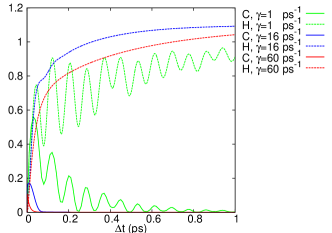
Figure 3: Delocalization $\mathcal{{H}}(\tau=N\Delta t)$ and coherence function $\mathcal{{C}}(\Delta t)$ for $\gamma=1,16,60$ $ps^{-1}$

We now focus on the relevant time scales $\tau_{d}$ for the initial fast delocalization process highlighted by our previous analysis, which are of the order of tens to hundreds of femtoseconds. We therefore introduce the following average measure of global coherence of the evolution

$$Q_{\tau_{d}}(\gamma)=\frac{1}{\tau_{d}}\int_{0}^{\tau_{d}}C(\Delta t)\,d\Delta t.$$

$Q_{\tau_{d}}(\gamma)$ is the average of the coherence exhibited by the dynamics of the system at the time scales $\Delta t\in(0,\tau_{d})$. In Fig. 4 we show $Q_{\tau_{d}}(\gamma)$ for the trimer (15) in the site basis for different values of $\tau_{d}$. We first focus on the behavior of $Q_{\tau_{d}}(\gamma)$ for values of dephasing in the range $\gamma\in(0,1)$ $ps^{-1}$. In this range, for small time scales $\tau_{d}=20$ to $200\,fs$ the average global coherence $Q_{\tau_{d}}(\gamma)$ is approximately constant and equals the value attained in the full quantum regime i.e., $Q_{\tau_{d}}(\gamma)\approx Q_{\tau_{d}}(\gamma=0.1)$ . For larger time scales ($\tau_{d}\approx 1\>ps$) $Q_{\tau_{d}}(\gamma)$ rapidly decreases with $\gamma$. This analysis shows that the behavior of $Q_{\tau_{d}}(\gamma)$ matches the expectations: the higher $\gamma$ the smaller the time scales over which decoherence takes place, the lower the global coherence of the dynamics. Along with $C(\Delta t)$ the functional $Q_{\tau_{d}}(\gamma)$ is therefore in general a good candidate for the evaluation of the global coherence of open quantum systems evolution. As for the transport dynamics, we focus on the timescale identified with the analysis of $\mathcal{{H}}(t)$ for optimal dephasing; for $\tau_{d}=\tau_{1}=20\,ps$ and $\tau_{d}=40\,ps$ we see that the system indeed retains most of the average coherence of the purely quantum regime up to the optimal values of decoherence ($\gamma=16\>ps^{-1}$ in the figure), losing it afterwards; this is a clear indication that this phenomenon is at the basis of the the fast initial delocalization process. Over longer time scales, the relevance of coherence is highly suppressed.

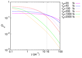
Figure 4: Average coherence of the evolution $Q_{\tau_{d}}(\gamma)$ for the trimer (15) for different values of $\tau_{d}$

We now deepen our analysis about the relevance of the coherence of the evolution for the energy tranfer efficiency. To this aim we focus on the basic feature that distingushes the classical and the quantum regime: interference. In particular we focus on the sub-block $\mathcal{D}_{3}$ of the decoherence matrix $\mathcal{D}$ pertaining to the third chromophore, which describes the set of histories in site basis ending at site $3$. Due to interference the probability of occupation of the site $3$ at time $\tau=N\Delta t$ can be written in terms of the the histories ending at site $3$ $p_{3}(\tau)=w_{3}(\tau)+\mathcal{I}_{3}(\mathbf{\tau})$, see (4) .

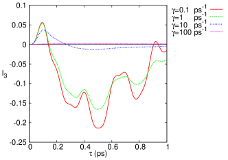
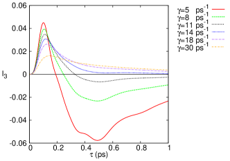
Figure 5: (a) interference $\mathcal{{I}}_{3}(\tau)$ of histories ending in site $3$ for the trimer (15) as a function of $\tau=N\Delta t$ for different values of $\gamma=0.1,1,10,100$; (b) $\mathcal{{I}}_{3}(\tau)$ for different intermediate values of $\gamma$

In Fig. 5 we show $\mathcal{I}_{3}(\tau)$ for different values of dephasing. One has different regimes: for $\gamma\gg 1$, the set of histories in site basis is fully decohered; $\mathcal{I}_{3}(\tau)\approx 0$, the histories do not interfere with each other and $p_{3}(\tau)\approx w_{3}(\tau)$ i.e, the probability is simply the sum of diagonal elements of $\mathcal{D}_{3}$. In the mainly quantum regime $\gamma\leq 1\,ps^{-1}$, $p_{3}(\tau)\neq w_{3}(\tau)$: after the initial positive peak the histories interfere with each other, globally the interference is mostly negative and therefore $p_{3}(\tau)\leq w_{3}(\tau)$. For intermediate values of decoherence $\gamma^{-1}\approx 10\>ps$ the interference has a positive peak and then reduces to zero. While the first initial fingersnap of positive interference that takes place in the first $\approx 80\>fs$ is common for all curves corresponding to small and intermediate values of $\gamma$, the main effect of the bath is displayed after this initial period of time: the decoherence gradually suppresses interference, both the positive and the negative one; however, for intermediate values of $\gamma$ the effect is stronger as for the negative part of the interference patterns. The environment thus implements what can be called a quantum recoil avoiding effect: it prevents the part of the exciton that – thanks to constructive interference – has delocalized on site $3$ to flow back to the the other sites.

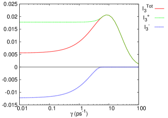
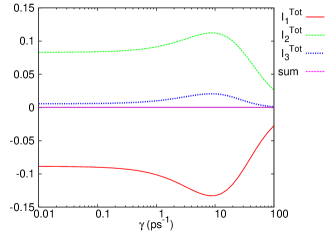
Figure 6: For the trimer (15) (a) Average positive (green), negative (blue), total (red) interference $\langle\mathcal{{I}}_{3}\rangle$ of histories ending in site $3$ as a function of $\gamma$; (b) total average interference $\langle\mathcal{{I}}_{i}^{Tot}\rangle$ for site $i=1$ (red), $i=2$ (blue), $i=3$ (green) $\gamma$.

In order to evaluate a possible advantage provided by the initial speed-up in the delocalization process and by the interference phenomena showed above one has to take into account another relevant time scale of the transport process: the trapping time. Indeed, if the system is to take advantage of the fast delocalization due to the coherent behavior, the exit of the exciton should take place on time scales of the order of the delocalization process. The theoretical and experimental evidences show that this is the case: the trapping time $\tau_{trap}=k_{trap}^{-1}$ for the FMO complex is estimated in the literature to be of the order of $0.2\>ps$ i.e., the exit of the exiton starts soon after the fast delocalization due to quantum coherence has taken place. The role of the interference between paths, in particular those leading to site $3$, can therefore be appreciated by numerically evaluating

$$\langle\mathcal{I}_{i}^{\beta}\rangle=\frac{{1}}{\tau_{trap}}\int_{0}^{\tau_{trap}}\mathcal{I}_{i}^{\beta}(\tau)d\tau$$ (17)

i.e., the average over the trapping time scale of $\tau_{trap}=200\>fs$ of the total ($\beta=Tot$), negative ($\beta=-$) and positive ($\beta=+$) average interference between the histories ending in site $i$, with $\langle\mathcal{I}_{i}^{Tot}\rangle=\langle\mathcal{I}_{i}^{+}\rangle+\langle\mathcal{I}_{i}^{-}\rangle$. In particular, in Fig. 6(a) the different kinds of interference are plotted for histories terminating at site $3$: on average, the negative interference highly reduces the total interference for small values of decoherence strength; when $\gamma\approx 10\>ps^{-1}$, $\langle\mathcal{I}_{3}^{-}\rangle$ vanishes, the average total interference equals the positive one $\langle\mathcal{I}_{3}^{Tot}\rangle=\langle\mathcal{I}_{3}^{+}\rangle$, and it is maximal for values of $\gamma$ comparable to those that maximize $\mathcal{{H}}(t)$ ($\approx 16\>ps^{-1}$). In Fig. 6(b), we compare the behavior of $\langle\mathcal{I}_{i}^{Tot}\rangle$ for all sites. The results again suggest that decoherence acts on the interference provided by the quantum engine in order to favor the flow of the exciton towards the exit chromophore: the average positive interference between histories ending at sites $2$ and $3$ grows in modulus with $\gamma$ and attains a maximum for intermediate values of decoherence; while the average negative interference between histories ending at site 1 decreases and attains a minimum for intermediate values of $\gamma$. The combined effect of decoherence and interference thus helps depopulating site 1 and populating site 2 and 3.

We can now tackle one of the most relevant aspects of our discussion: the net effect of the above described phenomena on the overall efficiency of the transport. The latter can be fully appreciated by evaluating the efficiency of the process (14) and by recognizing that, in the decoherent histories language, it can be expressed as:

$$\eta(t)=2k_{trap}\intop_{0}^{t}p_{3}(\tau)d\tau=W_{3}(t)+I_{3}(t)$$

where $\tau=N\Delta t$ and $W_{3}(t)=2k_{trap}\intop_{0}^{t}w_{3}(\tau)d\tau,\ I_{3}(t)=2k_{trap}\intop_{0}^{t}\mathcal{{I}}_{3}(\tau)d\tau$. This split allows one to appriciate the role of interference for the efficiency. In Fig. (7) $\eta$ is plotted for different values of dephasing. In agreement with what discussed above, we have three regimes: for very small values of $\gamma$ the overall efficiency is poor; this is due to the presence of high negative interference that in average prevents the exciton to migrate to the exit site. For large values of $\gamma$ the interference processes are completely washed out and the system cannot take advantage of the fast quantum delocalization. For intermediate (optimal) values of $\gamma$ only the negative interference has been washed out: $\mathcal{{I}}_{3}(\tau)$ is positive, it acts on short time scales, and it provides on average an enhancement of the global efficiency.

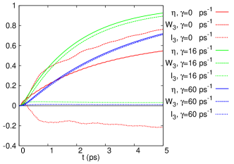
Figure 7: For the trimer (15): transport efficiency $\eta(t)$, integrated weight $W_{3}(t)=2k_{trap}\intop_{0}^{t}w_{3}(\tau)d\tau$ and integrated interference $I_{3}(t)=2k_{trap}\intop_{0}^{t}\mathcal{{I}}_{3}(\tau)d\tau$ for pathways ending at site $3$ for different values of $\gamma=0.1,16,60$ $ps^{-1}$ and $k_{trap}=5\,ps^{-1}$

These results, within the limits of the simple model of decoherence taken into account, undoubtedly show for the first time that the so called ENAQT phenomenon can well and properly be understood both qualitatively and quantitatively within the decoherence histories approach, i.e., in terms of very the basic concepts of coherence and interference between histories. The often recalled “convergence” of time scales or “Goldilocks” effect (Goldilocks ) in biological quantum transport systems seems therefore to be well rooted in the processes discussed above: if decoherence is too small the system shows both positive and negative interference (see Fig. 2), the delocalization has an ocillatory behavior, and the exciton bounces back and forth along the network thus preventing its efficient extraction. If instead decoherence is very high one has that the complete washing out of intereference and coherence implies the delocalization process to be very slow, no matter how fast the trapping mechanism try to suck the exciton out of the system. In order to take advantage of the effects of quantum coherent dynamics: $i)$ the bath must act on the typical time scales of quantum evolution in order to implement the quantum recoil avoiding process; $ii)$ the extraction of the exciton from the complex, characterized by $k_{trap}$, must then start soon after the initial fast delocalization has taken place. Should the extraction take place on longer time scales, the benefits of the fast initial delocalization would be spoiled: Waiting long enough, the system would eventually reach together with equilibrium a decent delocalization even for moderately high values of $\gamma$, but in this case the transfer would be obviously much slower.

V FMO

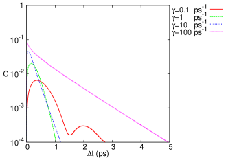
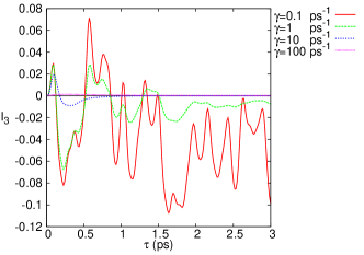
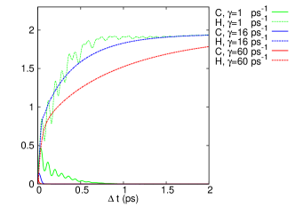
Figure 8: FMO: (a) $\mathcal{C}(\Delta t)$ for different values of $\gamma$; (b) $\mathcal{I}_{3}(\Delta t)$ for different values of $\gamma$; (c) $\mathcal{H}(\tau=N\Delta t),\mathcal{C}(\Delta t)$ for $\gamma=1,16,60\>ps^{-1}$;

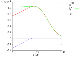
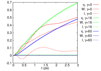
Figure 9: FMO: (a) average interference $<\mathcal{I}_{3}>$ for $k_{trap}=5\,ps^{-1}$; (b) transport efficiency $\eta(t)$, integrated weight $W_{3}(t)$ and integrated interference $I_{3}(t)$ for pathways ending at site $3$ for different values of $\gamma=0,1,16$ $ps^{-1}$ and $k_{trap}=5\,ps^{-1}$

The above arguments can be easily applied to the whole FMO complex. Fig. 8 and 9 show the application of the decoherent histories method to excitonic transport in FMO. The main features of the behavior of $\mathcal{{C}},\mathcal{{H}},\mathcal{{Q}},\mathcal{{I}}_{3}$ and $\eta$ are maintained although obvious differences can be found since the dynamics in now determined by the interplay of different eigenperiods and interference paths are more complex. In particular, Fig.8(b), one can observe a revival of positive interference $\mathcal{{I}}_{3}$ for small values of $\gamma\simeq 1$ , that does enhance the efficiency for $t\approx 1.5ps$, Fig. 9(a); but this is not sufficient to compensate the initial and subsequent negative interference, thus impeding the reach of optimal values of $\eta$. In general, compared to the trimer and as suggested by Fig. 9(a) the maximum average positive coherence on short time scales is attained for smaller values of $\gamma$. The overall picture is not significantly affected if one decides to start the dynamics from site $6$ instead of site $1$, as it often is reported in the literature.

VI Conclusions

The decoherent histories approach provides a general theory to study the distinctive feature exhibited by quantum systems: coherence. However, despite its generality and foundational character, in order to measure the effects of coherence and decoherence the DH approach needs to be complemented with a quantitative way to condense the information contained in the basic object of the theory, i.e., the decoherence matrix $\mathcal{D}$. In this paper we introduce a set of tools that allow one to assess the (global) coherence properties of quantum (Markovian) evolution and that can be used to relate the coherence content of a general quantum dynamical process to the relevant figure of merits of the given problem. We first define the coherence functional $C(P,N,\Delta t)$, that can be interpreted as a measure of the global coherence exhibited by the dynamics in the basis $P$ over the time scale $\Delta t$. While this measure is completely general, one can further introduce other relevant tools tailored to the specific system and type of system-environment interaction at hand. We thus focus on a simple yet paradigmatic model of environmentally assisted energy transfer where coherence effects have been shown to play a significant role in determining the efficiency of the process: a trimeric subunit of the Fenna-Matthews-Olson photosynthetic complex. Based on $\mathcal{D}$ and $C(P,N,\Delta t)$ we define: $a)$ a measure $\mathcal{Q}_{\tau}(\gamma)$ able to characterize the average coherence exhibited by the dynamics of the system over the time scales $\Delta t\in(0,\tau)$ for a fixed value of the dephasing $\gamma$; $b)$ a measure of the average interference $<\mathcal{I}_{i}>$ occurring between the histories ending at a given “site” $i$.
Within the specific model, we first thoroughly assess the consistency of the behavior of $C(P,N,\Delta t)$ in the various regimes. We then show how the introduced tools allow to study the intricate connections between the efficiency of the transport process and the coherence properties of the dynamics. In particular we show that the delocalization of the exciton over the chromophoric subunit is strongly affected by the amount of (average) coherence allowed by the interaction with the bath in the first tens to hundreds of femtoseconds. If the system-bath interaction is too strong, coherence is suppressed alongside the interference between different histories, in particular those ending at the site where the excitation leaves the complex. If the interaction is too weak the system exhibits high values of coherence even on long time scales, but it also exhibits negative interference between pathways ending at the exit site, a manifestation of the fact that the exciton bounces back and forth over the network thus preventing its efficient extraction. In the intermediate regime i.e., when the different time scales of the system (quantum oscillations, decoherence and trapping rate) converge, the system shows high values of coherence on those time scales. The action of the bath has a quantum recoil avoiding effect on the dynamics of the excitation: the benefits of the fast initial quantum delocalization of the exciton over the network are preserved and sustained in time by the dynamics; in terms of pathways leading to the exit site, the action is to selectively kill the negative interference between pathways, while retaining the initial positive one. These effects can be explicitly connected to the overall efficiency of the environment-assisted quantum transport: the gain in efficiency for intermediate (optimal) values of decoherence can thus be traced back to the basic concepts of coherence and interference between pathways as expressed in the decoherent histories language.
While the specific decoherence model used (Haken-Strobl) is an oversimplified description of the actual dynamics taking place in real systems, we believe that our analysis allows to spot out the essential features that may determine the high efficiency of the transport even in more complex system-environment scenarios.
In conclusion, the tools introduced in this paper allow to thoroughly assess the coherence properties of quantum evolutions and can be applied to a large variety of quantum systems, the only limits being the restriction to Markovian dynamics and the computational efforts required for high dimensional systems. However, the extension to non-Markovian realms is indeed possible Allegraprep , and the use of parallel computing may allow the treatement of reasonably large systems.

References

- (1) R. B. Griffiths, J. Stat. Phys. 36, 219 (1984).
- (2) R. B. Griffiths, Consistent quantum theory, Cambridge University Press (2003).
- (3) M. Gell-Mann and J. B. Hartle, Phys.Rev. D 47, 3345 (1993).
- (4) M. Gell-Mann and J. B. Hartle, in Complexity, entropy, and the physics of information (Addison-Wesley, Reading, Massachusetts, 1990); in Proc. of the 25th International Conference on High Energy Physics, Singapore (World Scientific, Singapore, 1990).
- (5) M. Gell-Mann and J. B. Hartle. Physical Review A 89, 052125 (2014).
- (6) J. B. Hartle, Phys. Rev. A 78, 012108 (2008).
- (7) W. H. Zurek, J. P. Paz, Phys. Rev. D 48, 2728 (1993).
- (8) R. Omnès, J. Stat. Phys. 53, 893, 933, 957 (1988), 57, 357 (1989); Rev. Mod. Phys. 64, 339 (1992);
- (9) A. Ishizaki, T. R Calhoun,G. S. Schlau-Cohen, and G. R. Fleming, Phys. Chem. Chem. Phys. 12, 7319 (2010).
- (10) A. Ishizaki, and G. R. Fleming, Proc. Natl. Acad. Sci. USA 106, 17255 (2009).
- (11) H. Park, N. Heldman, P. Rebentrost, L. Abbondanza, A. Iagatti, A. Alessi, B. Patrizi, M. Salvalaggio, L. Bussotti, M. Mohseni, F. Caruso, H. C. Johnsen, R. Fusco, P. Foggi, P. F. Scudo, S. Lloyd & A. M. Belcher, Nature Materials (2015).
- (12) L. Banchi, G. Costagliola, A. Ishizaki, and P. Giorda, J. Chem. Phys. 138, 184107 (2013).
- (13) K. M. Gaab and C. J. Bardeen, J. Chem. Phys. 121, 7813 (2004).
- (14) R.E. Blankenship, Molecular Mechanisms of Photosynthesis, Blackwell Science Ltd., London (2002).
- (15) G.S. Engel, T. R. Calhoun, E. L. Read, T. K. Ahn, T. Mancal, Y. C. Cheng, R. E. Blankenship and G. R. Fleming, Nature 446, 782 (2007).
- (16) E. Collini, C. Y.Wong, K. E.Wilk, P.M. Curmi, P. Brumer, and G. D. Scholes, Nature 463, 644 (2010).
- (17) G. Panitchayangkoon, D. Hayes, K. A. Fransted, J. R. Caram, E. Harel, J. Wen, R. E. Blankenship, G. S. Engel, Proc. Nat. Acad. Sci. 107, 12766 (2010).
- (18) M. Mohseni, P. Rebentrost, S. Lloyd, and A. Aspuru-Guzik, J. Chem. Phys. 129, 174106 (2008).
- (19) P. Rebentrost, M. Mohseni, I. Kassal, S. Lloyd, and A. Aspuru- Guzik, New J. Phys. 11, 033003 (2009).
- (20) M.B. Plenio and S.F. Huelga, New J. Phys. 10, 113019 (2008).
- (21) J.M. Moix, M. Khasin, J. Cao, New Journal of Physics 15, 085010 (2013)
- (22) S. Lloyd, M. Mohseni, A. Shabani, H. Rabitz, arXiv:1111.4982 (2011).
- (23) H. Haken, G. Strobl, in The Triplet State, Proceedings or the International Symposium, Am. Univ. Beirut, Lebanon (1967), A.B. Zahlan, ed., Cambridge University Press, Cambridge (1967); H. Haken, P. Reineker, Z. Phys. 249, 253 (1972).
- (24) M. Cho, H. M. Vaswani, T. Brixner, J. Stenger, and Gr. R. Fleming, J. Phys. Chem. B 109, 10542-10556 (2005).
- (25) J. Adolphs and T. Renger, Biophysical Journal 91, 2778-2797 (2006).
- (26) F. Caruso, A.W. Chin, A. Datta, S.F. Huelga, M.B. Plenio, Phys. Rev. A 81, 062346 (2010).
- (27) M. Sarovar, A. Ishizaki, G.R. Fleming, K.B. Whaley, Nat. Phys. 6, 462 (2010).
- (28) P. Giorda, S. Garnerone, P. Zanardi, S. Lloyd, arXiv:1106.1986 (2011).
- (29) A. Ishizaki and G. R. Fleming, New J. Phys. 12, 055004 (2010).
- (30) M. Tiersch, S. Popescu and H. J. Briegel, Phil. Trans. R. Soc. A, 370, 1972, 3771-3786 (2012).
- (31) W. H. Miller, J. Chem. Phys. 136, 210901 (2012).
- (32) for a definion and discussion of coherence in quantum states, see T. Baumgratz, M. Cramer, and M. B. Plenio Phys. Rev. Lett. 113, 140401 (2014) and references therein.
- (33) M. Allegra, P. Giorda and S. Lloyd, in preparation.