Supplementary Material for ”Exotic attractors of the non-equilibrium Rabi-Hubbard model”

The supplementary material is organized as follows: Section I presents further details of the possible explicit driving scheme realizing a (tunable) Rabi-Hubbard model as presented in Eq. (1) of the main text. Section II presents the mean field and linear stability results for the generalized Rabi-Hubbard, with $g^{\prime}\neq g$ that were mentioned in the main text. Section III discusses the construction of the effective spin model introduced in the main text and the linear stability analysis of this model. Section IV presents further results on the effective spin model obtained by MPO simulations of an infinite chain.

I Raman Driving Scheme and Tunable Rabi Hubbard

In this section we present a possible scheme to obtain the Rabi Hubbard model starting from a driven four-level atom in a cavity. This scheme follows closely the original proposal Dimer et al. (2007) for a driven realisation of the generalized Dicke model, which was recently experimentally realized Baden et al. (2014). To show most clearly how Rabi-like interactions can be generated from multi-atom driven problem we focus here on the isolated single cavity Hamiltonian, and disregard for now the photon hopping to other neighboring resonators. The interference between coupling to other cavities and pump induced terms can generate very weak long-ranged hopping and interactions between cavities. The analysis of these small corrections is left for future studies.

Our starting point is thus a four-level (artificial) atom in an optical cavity (or microwave resonator), supporting a single photon mode, see Figure 1. The full local Hamiltonian is made of several terms. The non-interacting atom and cavity are described by

$$\hat{H}_{0}=\omega_{\text{cav}}\,\hat{a}^{\dagger}\hat{a}+\sum_{j=0,1,r,s}\,E_{j}\,|\,j\rangle\langle\,j|.$$

Following Ref. Dimer et al., 2007 we consider a case where the cavity mode drives transitions between the states $|0\rangle\leftrightarrow|\,r\rangle$ and $|1\rangle\leftrightarrow|\,s\rangle$. Selecting these transitions can either be done by tuning the other transitions to be far off resonance with the cavity mode, or ideally, by engineering a system with selection rules restricting which transitions the cavity mode polarisation couples to Baden et al. (2014). The resulting cavity-atom coupling Hamiltonian reads:

$$\hat{H}_{\text{int}}=g_{r}\,|\,r\rangle\langle\,0|\,\hat{a}+g_{s}\,|\,s\rangle\langle\,1|\,\hat{a}+\text{H.c.}$$

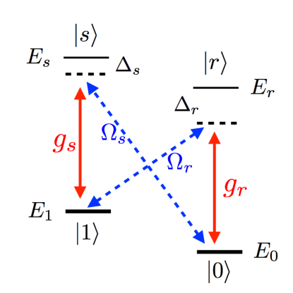
Figure 1: Cartoon of the level structure and Raman driving scheme to engineer a tunable Rabi Hamiltonian.

Since the goal is to generate effective light-matter interactions between the photon and the low-lying doublet $|\,0\rangle,|\,1\rangle$, we need to connect these states through resonant two-photon transitions. This can be done by adding the drive term:

$$\hat{H}_{\text{drive}}(t)=\frac{\Omega_{r}}{2}\,e^{-i\omega_{r}^{p}\,t}\,|\,r\rangle\langle\,1|+\frac{\Omega_{s}}{2}\,e^{-i\omega_{s}^{p}\,t}\,|\,s\rangle\langle\,0|+\text{H.c.}$$

A cartoon of the level scheme, and the pump- and cavity-mediated transitions is shown in Figure 1.

The crucial feature of this scheme is that the laser drives transitions between $|1\rangle\leftrightarrow|\,r\rangle$ and $|0\rangle\leftrightarrow|\,s\rangle$ so that the combined effect of $H_{\text{int}}$ and $H_{\text{drive}}$ is to induce two-photon transitions between $|\,0\rangle$ and $|\,1\rangle$, involving emission or absorption of a cavity photon. These will become the familiar rotating and counter-rotating terms of the Rabi model.

We proceed in two steps, that we briefly outline here. First, we eliminate the explicit time dependence of the drive by performing an unitary transformation to a rotating (comoving) frame. This can be implemented by the operator:

$$\hat{\Omega}(t)=\exp\left(-i\hat{K}t\right),\quad\hat{K}=\alpha\,\hat{a}^{\dagger}\hat{a}+\sum_{i}\,\beta_{i}|\,i\rangle\langle\,i|,$$

which has the property that, $\hat{\Omega}^{\dagger}(t)\,\hat{a}\,\hat{\Omega}(t)=\hat{a}e^{-i\alpha t}$ and $\hat{\Omega}^{\dagger}(t)\,|\,i\rangle\langle\,j|\,\hat{\Omega}(t)=|\,i\rangle\langle\,j|\,e^{i\left(\beta_{i}-\beta_{j}\right)t}$. We can fix the parameters in $\hat{K}$ in such a way that the transformed Hamiltonian $\tilde{H}=i\partial_{t}\left(\hat{\Omega}^{\dagger}(t)\right)\hat{\Omega}(t)+\hat{\Omega}^{\dagger}(t)\,\hat{H}(t)\,\hat{\Omega}(t)$, with $\hat{H}=\hat{H}_{0}+\hat{H}_{\text{int}}+\hat{H}_{\text{drive}}$, becomes time-independent. We stress that while the problem in this new rotating frame is now fully time-independent, it remains intrinsically out of equilibrium in nature since (i) we are forced to study the dynamics of $\tilde{H}$, and (ii) the distribution function of any bath modes the system couples to becomes strongly non-thermal (breaking detailed balance between gain and loss), as the unitary transform $\hat{\Omega}$ must also be applied to the system-bath coupling.

We now proceed to the elimination of atomic excited states $|\,r\rangle,|\,s\rangle$ in order to obtain an Hamiltonian for the manifold $|\,i\rangle=|\,0\rangle,|\,1\rangle$ that will play the role of our qubit. This can be done perturbatively, using a Schrieffer-Wolf transformation, $\tilde{H}_{\text{S}}=e^{i\hat{S}}\tilde{H}e^{-i\hat{S}}$ with a generator $\hat{S}$ coupling the qubit manifold $|0\rangle,|1\rangle$ to the excited states $|r\rangle,|s\rangle$

$$\hat{S}=i\biggl{(}\frac{\Omega_{r}}{2\Delta_{r}}|r\rangle\langle 1|+\frac{\Omega_{s}}{2\Delta_{s}}|s\rangle\langle 0|+\\ +\frac{g_{r}}{\Delta^{\omega}_{r}}\,\hat{a}|r\rangle\langle 0|+\frac{g_{s}}{\Delta^{\omega}_{s}}\,\hat{a}|s\rangle\langle 1|\biggr{)}+H.c..$$

This is obtained by imposing the condition $[\hat{H}_{0},i\hat{S}]=\hat{H}_{\text{int}}+\hat{H}_{\text{drive}}$ (in terms of the time-independent Hamiltonian). We have introduced the detunings

$$\Delta^{\omega}_{r} =\omega_{\text{cav}}+E_{0}-E_{r},$$

$$\Delta^{\omega}_{s} =\omega_{\text{cav}}+E_{1}-E_{s}+(\omega^{s}_{p}-\omega_{p}^{r})/2,$$

$$\Delta_{r} =E_{1}-E_{r}+\omega_{p}^{r},\qquad\Delta_{s}=E_{0}-E_{s}+\omega_{p}^{s}.$$

To leading order in the strength of the drive and light-matter coupling we get $\tilde{H}_{\text{S}}=\tilde{H}_{\text{Rabi}}+\mathcal{O}(g_{r}/\Delta_{r},g_{s}/\Delta_{s},\Omega_{r}/\Delta_{r},\Omega_{s}/\Delta_{s})$ where

$$\tilde{H}_{\text{Rabi}}=\omega\,\hat{a}^{\dagger}\hat{a}+\frac{\omega_{0}}{2}\hat{\sigma}^{z}+\lambda\,\hat{a}^{\dagger}\hat{a}\hat{\sigma}^{z}+g(\hat{a}^{\dagger}\hat{\sigma}^{-}+\hat{a}\hat{\sigma}^{+})\\ +g^{\prime}(\hat{a}^{\dagger}\hat{\sigma}^{+}+\hat{a}\hat{\sigma}^{-}).$$ (1)

This is a generalized Rabi model, for which the parameters depend on the frequency and strength of the external drive as follows:

$$\omega =\omega_{cav}+\frac{1}{2}\left(\frac{g^{2}_{r}}{\Delta^{\omega}_{r}}+\frac{g^{2}_{s}}{\Delta^{\omega}_{s}}\right)-\frac{\omega^{s}_{p}+\omega^{r}_{p}}{2},$$

$$\omega_{0} =E_{1}-E_{0}+\frac{1}{8}\left(\frac{\Omega^{2}_{r}}{\Delta_{r}}-\frac{\Omega^{2}_{s}}{\Delta_{s}}\right)-\frac{\omega^{s}_{p}-\omega^{r}_{p}}{2},$$

$$\lambda =\frac{1}{2}\left(\frac{g^{2}_{r}}{\Delta^{\omega}_{r}}-\frac{g^{2}_{s}}{\Delta^{\omega}_{s}}\right),\quad g=\frac{g_{r}\Omega_{r}}{2\bar{\Delta}_{r}},\quad g^{\prime}=\frac{g_{s}\Omega_{s}}{2\bar{\Delta}_{s}},$$

where we defined $1/\bar{\Delta}_{r/s}=1/\Delta^{\omega}_{r/s}+1/\Delta_{r/s}$.

To complete the mapping to the generalized Rabi model we must choose parameters such that the coefficient $\lambda=0$, as also discussed in Dimer et al. (2007). To this end we note that $\Delta^{\omega}_{r}$ is drive-independent and therefore fixed by the physical realization, while $\Delta^{\omega}_{s}$ can be tuned by $\omega^{s}_{p}$. We therefore impose the condition:

$$\Delta^{\omega}_{s}=\Delta^{\omega}_{r}\frac{g_{s}^{2}}{g_{r}^{2}},\qquad$$

which immediately gives $\lambda=0$. From this we see that we may want to have $g_{s}/g_{r}\sim 1$ in order to have both $\Delta^{\omega}_{r},\Delta^{\omega}_{s}$ large. The second drive frequency $\omega^{r}_{p}$ can then be used to control the effective detuning between the qubit and the resonator. In addition to changing the detuning through the pump frequencies, we can vary the pump strengths $\Omega_{r},\Omega_{s}$ to tune (independently) the relative strengths of the rotating and counter-rotating terms.

II Open Rabi Hubbard for $g^{\prime}\neq g$

In this section we present results, anticipated in the main text, for the phase diagram of the generalized open Rabi Hubbard, with $g^{\prime}\neq g$. We use again linear stability analysis of the normal phase, as described in the main text, and plot in figure 2 the phase boundary in the $(g,J)$ plane and, in color scale, the wavevector of the most unstable mode, for two different values of $g^{\prime}/g$, respectively $g^{\prime}=0.5g$ (left panel) and $g^{\prime}=0.25g$ (right panel). These results show several interesting features. Firstly there is a change in the topography of the phase boundary, with multiple separate ordered regions, as opposed to the case $g^{\prime}=g$ which features a single, connected, broken symmetry phase. As a result, upon increasing the light-matter interaction $g$ one can have a sequence of transitions, where the symmetry is broken first, then restored and then broken again. In addition, for smaller values of the ratio $g^{\prime}/g$ the nature of the ordered phase changes qualitatively and an instability at $k=\pi$, eventually emerges. This corresponds to an antiferroelectric (AF) order, where photon and two-level system (qubit) polarization changes sign between neighboring sites. This latter result is particularly striking if interpreted in terms of equilibrium physics. Indeed the effective qubit-qubit interaction mediated by a population of photon modes in equilibrium at zero temperature would be negative at short distance Schiró et al. (2012) leading to a uniform ferroelectric pattern in the ground state. The results of figure 2 show the profound differences between the open driven-dissipative and equilibrium incarnations of the Rabi Hubbard model. As we have discussed in the main text, these intriguing results can be understood qualitatively in terms of an effective open-dissipative spin model whose construction we are now going to discuss in detail in the rest of this supplementary material.

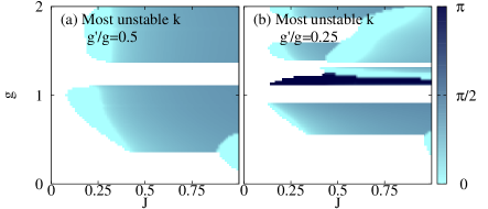
Figure 2: Mean field phase diagram of the generalized ($g^{\prime}\neq g$) open Rabi Hubbard model as obtained from the linear stability analysis of the normal phase. We plot the phase boundary in the $(g,J)$ plane and, in color scale, the wavevector of the most unstable mode, for two different values of $g^{\prime}/g$, respectively $g^{\prime}=0.5g$ (left panel) and $g^{\prime}=0.25g$ (right panel).

III Effective Spin Model

By truncating the on-site Rabi model ($\tilde{H}_{\text{Rabi}}$ obtained in the previous section) to the lowest two eigenstates and labelling these as $|\pm\rangle_{n}$ (with corresponding energies $E_{\pm}$) to denote their different parities, we obtain the following low-frequency effective Master equation describing the dynamics of the generalized Rabi-Hubbard model:

$$\partial_{t}\rho=-i[\hat{H}^{\text{\text{eff}}},\rho]+\kappa\mathcal{L}[A_{-}\hat{\tau}_{n}^{-}+A_{+}\hat{\tau}_{n}^{+},\rho]+\\ +\gamma\mathcal{L}[S_{-}\hat{\tau}_{n}^{-}+S_{+}\hat{\tau}_{n}^{+},\rho],$$ (2)

where the effective Hamiltonian for the generalized Rabi-Hubbard Model reads (for a detailed discussion of this projection, see Refs. Schiró et al., 2012, 2013 which discuss the case $g=g^{\prime}$)

$$\hat{H}^{\text{\text{eff}}}=\frac{\Delta}{2}\sum_{n}\hat{\tau}^{z}_{n}\\ -J\sum_{\langle n,m\rangle}\left(A_{-}\hat{\tau}^{+}_{n}+A_{+}\hat{\tau}^{-}_{n}\right)\left(A_{-}\hat{\tau}^{-}_{m}+A_{+}\hat{\tau}^{+}_{m}\right),$$

where $\hat{\tau}_{n}^{i}$ are Pauli matrices on the $n$th site, $\Delta=E_{+}-E_{-}$ is the lowest excitation energy of the local Rabi model, and we have introduced the real-valued coefficients

$$A_{\pm}={}_{n}\langle\pm|\hat{a}_{n}|\mp\rangle_{n},\qquad S_{\pm}={}_{n}\langle\pm|\hat{\sigma}^{-}_{n}|\mp\rangle_{n}.$$ (3)

For later convenience it is useful to introduce the even and odd combinations of these coefficients, namely

$$\alpha_{\pm}=A_{+}\pm A_{-},\;\qquad\;\varsigma_{\pm}=S_{+}\pm S_{-}.$$ (4)

The effective-model parameters $\Delta,\alpha_{\pm},\varsigma_{\pm}$ are functions of the parameters $g,g^{\prime},\omega_{0}$ in the Rabi model. We will discuss below analytic approximations in the limit of large $g=g^{\prime}$, the effective model is however useful more generally.

III.1 Mean-field theory, linear stability

The effective model can be used to find a closed-form expression for the critical hopping required to stabilize the ordered state within the mean-field theory, as discussed next. Within a mean-field decoupling of the hopping, the single site Hamiltonian has the form

$$\hat{H}^{\text{eff,MF}}_{n}=\frac{\Delta}{2}\hat{\tau}^{z}_{n}-\frac{J}{4}\alpha_{+}^{2}\,\hat{\tau}^{x}_{n}\,h^{x}_{n}-\frac{J}{4}\alpha_{-}^{2}\,\hat{\tau}^{y}_{n}\,h^{y}_{n},$$ (5)

where the local effective fields

$$h^{x}_{n}=\sum_{m:\langle mn\rangle}x_{m},\,\qquad\,h^{y}_{n}=\sum_{m:\langle mn\rangle}y_{m},,$$

are written in terms of $x_{n}=\langle\hat{\tau}^{x}_{n}\rangle,y_{n}=\langle\hat{\tau}^{y}_{n}\rangle,z_{n}=\langle\hat{\tau}^{z}_{n}\rangle$, account for the effect of the sites $m$ connected by photon hopping to sites $n$. By introducing the damping rates

$$\Gamma_{\pm}=\kappa\alpha_{\pm}^{2}+\gamma\varsigma_{\pm}^{2},$$

and the normal state inversion

$$z_{0}=\frac{2}{\Gamma_{+}+\Gamma_{-}}\left(\kappa\alpha_{+}\alpha_{-}+\gamma\varsigma_{+}\varsigma_{-}\right),$$

we can write down the mean field dynamics in a compact form as

$$\partial_{t}x_{n} =-\Delta y_{n}-\Gamma_{-}x_{n}-\frac{J}{2}\alpha_{-}^{2}\,h^{y}_{n}\,z_{n},$$

$$\partial_{t}y_{n} =\Delta x_{n}-\Gamma_{+}y_{n}+\frac{J}{2}\alpha_{+}^{2}\,h^{x}_{n}\,z_{n},$$

$$\partial_{t}z_{n} =\left(\Gamma_{+}+\Gamma_{-}\right)\left(z_{0}-z_{n}\right)-\frac{J}{2}\alpha_{-}^{2}\,h^{x}_{n}\,y_{n}+\frac{J}{2}\alpha_{-}^{2}\,h^{y}_{n}\,x_{n}.$$

The normal state solution is given by $z_{n}=z_{0}$ and $x_{n}=y_{n}=0$. Considering small fluctuations about this stationary solution we obtain a decoupled equation for $z_{n}$, with damping rate $\Gamma_{+}+\Gamma_{-}$ while for the other components the ansatz $x_{n}=\sum_{{\bm{k}}}\,x_{{\bm{k}}}\,e^{i\left({\bm{k}}\cdot{\bm{n}}-\nu_{{\bm{k}}}t\right)}$ gives the secular equation for the frequencies $\nu_{{\bm{k}}}$,

$$(i\nu_{{\bm{k}}}-\Gamma_{-})(i\nu_{{\bm{k}}}-\Gamma_{+})+\left(\Delta-t_{\bm{k}}\alpha_{+}^{2}z_{0}\right)\left(\Delta-t_{\bm{k}}\alpha_{-}^{2}z_{0}\right)=0,$$

where $t_{{\bm{k}}}=-2J\sum_{i=1}^{d}\cos(k_{i})$ is the $d$-dimensional bare photon dispersion. The instability, corresponding to a pitchfork bifurcation, is given by $\nu_{{\bm{k}}}=0$. This leads to a simple expression for the critical $J$ in the limit $|\alpha_{-}|\ll|\alpha_{+}|$, which, as we will see, is satisfied at large $g=g^{\prime}$. For the case where a ferromagnetic (anti-ferromagnetic) instability ${k}_{i}=0(\pi)$ occurs, this expression is:

$$J_{crit}=\mp\frac{1}{2d\alpha_{+}^{2}z_{0}}\left(\Delta+\frac{\Gamma_{+}\Gamma_{-}}{\Delta}\right).$$ (6)

Since we consider only positive $J$, it is clear from the form of this equation that the sign of $t_{{\bm{k}}}$ required, i.e. whether the instability is ferro (F) or antiferro (AF), is determined by the sign of the product $\Delta z_{0}$. For $g=g^{\prime}$, we always have $\Delta>0,z_{0}<0$ and so only the ferromagnetic case (negative sign) occurs Thus, as discussed in the main text, the level crossing at $\Delta=0$, and the inversion point at $z_{0}=0$ lead to suppression of ordering, and a switch between F and AF ordering.

III.2 Large $g$ limit and Effective Model parameters

In the limit of large $g=g^{\prime}$ one may use an approximate solution of the on-site Rabi model to derive simple analytic expressions for the lowest excitation energy $\Delta$ and the matrix elements $\alpha_{\pm},\varsigma_{\pm}$. To extract these expressions we start from the single site Rabi Hamiltonian

$$\hat{H}^{\text{Rabi}}=\frac{\omega_{0}}{2}\hat{\sigma}^{z}+\omega\hat{a}^{\dagger}\hat{a}+g(\hat{a}^{\dagger}+\hat{a})\hat{\sigma}^{x},$$ (7)

and perform the unitary transformation

$$\hat{U}=\exp\left[-\hat{X}\hat{\sigma}^{x}\right],\,\qquad\,\hat{X}=\frac{g}{\omega}(\hat{a}^{\dagger}-\hat{a}),$$

to obtain $\tilde{H}^{\text{Rabi}}=\hat{U}^{\dagger}\hat{H}^{\text{Rabi}}\hat{U}$ in the form

$$\tilde{H}^{\text{Rabi}}=-\frac{g^{2}}{\omega}+\omega\hat{a}^{\dagger}\hat{a}+\frac{\omega_{0}}{2}\left[\cosh 2\hat{X}\,\hat{\sigma}^{z}-i\sinh 2\hat{X}\,\hat{\sigma}^{y}\right].$$ (8)

In absence of the term in brackets the spectrum has an infinite sequence of two-fold degenerate states with energies $E^{0}_{n}=-(g^{2}/\omega)+n\omega$ and corresponding eigenstates $|\sigma=\{\uparrow,\downarrow\},n\rangle$ in the transformed basis. In what follows we carry out a perturbation expansion in $\delta\hat{H}=\frac{\omega_{0}}{2}\left[\cosh 2\hat{X}\,\hat{\sigma}^{z}-i\sinh 2\hat{X}\,\hat{\sigma}^{y}\right]$ for the states in the lowest manifold (identified by $n=0$). This is justified by the smallness of the parameter $\langle 0|e^{\pm 2\hat{X}}|0\rangle=\exp\left(-2(g/\omega)^{2}\right)$ in the large-g limit $g/\omega\gg 1$. To lowest order, this splits the $n=0$ doublet and yields an analytic expression for the lowest excitation energy of the Rabi model:

$$\Delta=\omega_{0}\exp\left(-2g^{2}/\omega^{2}\right).$$ (9)

To obtain an analytic expression for the matrix elements Eq. 4, we also need to compute the first order correction to the wavefunctions $|\sigma,0\rangle$:

$$|\widetilde{{\sigma},0}\rangle=|{\sigma},0\rangle-\sum_{n>0,\tau}\frac{|{\tau},n\rangle\langle\tau,n|\delta\hat{H}|{\sigma},0\rangle}{n\omega},$$ (10)

where $|\widetilde{\sigma,0}\rangle$ denotes the corrected wavefunction, and the matrix elements of the perturbation Hamiltonian can be found using the following expression:

$$\langle n|\delta\hat{H}|0\rangle =\frac{\omega_{0}}{2}\langle n|\cosh(2\hat{X})\hat{\sigma}_{z}-i\sinh(2\hat{X})\hat{\sigma}_{y}|0\rangle$$

$$=\frac{\Delta}{2\sqrt{n!}}\left(\frac{2g}{\omega}\right)^{n}\left[I_{n\in even}\,\hat{\sigma}_{z}-i\,I_{n\in odd}\,\hat{\sigma}_{y}\right].$$ (11)

where $I_{n\in A}$ is an indicator function, taking value $1$ for $n\in A$ and zero elsewhere.

We can now evaluate the matrix elements of photon and spin operators in the space spanned by the low-energy doublet, that in the transformed basis are simply the states $|\uparrow,0\rangle,|\downarrow,0\rangle$. To evaluate the spin matrix elements we note that, under the unitary transformation we have

$$\hat{U}^{\dagger}\hat{\sigma}^{-}\hat{U}=\frac{1}{2}\left[\hat{\sigma}_{x}+\cosh(2\hat{X})(-i\hat{\sigma}_{y})+\sinh(2\hat{X})\hat{\sigma}_{z}\right],$$ (12)

from which we conclude that

$$S_{+} =\langle\uparrow,0|\hat{U}^{\dagger}\hat{\sigma}^{-}\hat{U}|\downarrow,0\rangle=\frac{1}{2}\left(1-\frac{\Delta}{\omega_{0}}\right),$$ (13)

$$S_{-} =\langle\downarrow,0|\hat{U}^{\dagger}\hat{\sigma}^{-}\hat{U}|\uparrow,0\rangle=\frac{1}{2}\left(1+\frac{\Delta}{\omega_{0}}\right),$$ (14)

where to leading order we have only accounted for the transformation of the operator. Turning to the photon matrix elements we first note that under the unitary transformation we have

$$\hat{U}^{\dagger}\hat{a}\hat{U}=\hat{a}-\frac{g}{\omega}\hat{\sigma}_{x},$$ (15)

therefore to evaluate the matrix element one has to use the perturbed eigenstate to obtain, at leading order,

$$A_{+}=\langle\widetilde{\uparrow,0}|\hat{a}-\frac{g}{\omega}\hat{\sigma}_{x}|\widetilde{\downarrow,0}\rangle=\frac{g\Delta}{\omega^{2}}-\frac{g}{\omega},,\quad A_{-}=-\frac{g\Delta}{\omega^{2}}-\frac{g}{\omega}.$$ (16)

Using these results, we find that the matrix elements can be found to leading order to be $\alpha_{+}=2g/\omega,\alpha_{-}=2g\Delta/\omega^{2},\varsigma_{+}=1,\varsigma_{-}=\Delta/\omega_{0}$, from which we can obtain the approximate expression for the critical boundary given in the main text.

IV MPO Results for the Rabi Hubbard case, $g=g^{\prime}$

In order to test the predictions of mean-field theory, we may use a infinite Matrix-Product Operator (iMPO) approach Vidal (2003, 2004); Zwolak and Vidal (2004); Schollwöck (2011) to find the non-equilibrium steady state of the effective model, supplementary Eq. (2). The iMPO approach is applicable to a translationally invariant problem Orús and Vidal (2008), allowing one to evolve only a representative pair of sites, and has no finite-size effects. Despite this, as seen in Fig. 5 of the paper, iMPO can fully describe inhomogeneous order; this is because multi-site expectations involve traces of products of the representative matrix. Our approach, as in previous work Joshi et al. (2013), is to simulate an adiabatic sweep, starting from the point $g=g^{\prime}=0$ where the state is trivially a product state. Such a sweep avoids the high transient entanglement that occurs with a quench of parameters, and means that the correlation functions we measure are converged for the bond dimension $\chi=120$ we use.

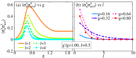
Figure 3: Correlations of the one-dimensional effective spin $1/2$ model, evaluated in an infinte-MPO approach for $g^{\prime}=g=1,J=0.5$ (a) Correlations vs $g$, at various separations $l$ between sites. (b) Correlations vs separation at various values of $g$.

In the main text we showed results for $g^{\prime}/g=0.25$, illustrating that the F-AF-F sequence predicted by mean-field theory still exists (albeit short-ranged) for the MPO simulation. Here we present additional MPO results on the effective spin model in the pure Rabi case, i.e. for $g=g^{\prime}=1$. In particular the data reported in figure 3 show short-ranged ferroelectric correlations developing for several values of the light-matter interaction, consistently with the mean field picture.

References

- Dimer et al. (2007) F. Dimer, B. Estienne, A. S. Parkins, and H. J. Carmichael, Phys. Rev. A 75, 013804 (2007).
- Baden et al. (2014) M. P. Baden, K. J. Arnold, A. L. Grimsmo, S. Parkins, and M. D. Barrett, Phys. Rev. Lett. 113, 020408 (2014).
- Schiró et al. (2012) M. Schiró, M. Bordyuh, B. Öztop, and H. E. Türeci, Phys. Rev. Lett. 109, 053601 (2012).
- Schiró et al. (2013) M. Schiró, M. Bordyuh, B. Öztop, and H. E. Türeci, J. Phys. B: At. Mol. Opt. Phys. 46, 224021 (2013).
- Vidal (2003) G. Vidal, Phys. Rev. Lett. 91, 147902 (2003).
- Vidal (2004) G. Vidal, Phys. Rev. Lett. 93, 040502 (2004).
- Zwolak and Vidal (2004) M. Zwolak and G. Vidal, Phys. Rev. Lett. 93, 207205 (2004).
- Schollwöck (2011) U. Schollwöck, Annals of Physics 326, 96 (2011), january 2011 Special Issue.
- Orús and Vidal (2008) R. Orús and G. Vidal, Phys. Rev. B 78, 155117 (2008).
- Joshi et al. (2013) C. Joshi, F. Nissen, and J. Keeling, Phys. Rev. A 88, 063835 (2013).