Towards the large volume limit – A method for lattice QCD + QED simulations

Abstract:

We present a method to couple finite-volume QCD to infinite-volume QED by an appropriate twist-averaging procedure. We demonstrate the prescription numerically for the leading-order hadronic contribution to the anomalous magnetic moment of the muon and the electro-magnetic pion mass splitting.

1 Motivation

The long-distance nature of QED poses a substantial challenge when including QED interactions in lattice QCD simulations. While it is possible to account analytically for the large power-law corrections that are introduced by the QED interaction in finite-volume QCD+QED simulations, see, e.g., [1, 2], such a setup requires the use of lattice ensembles that are much larger than necessary for a pure QCD simulation. An alternative procedure that explicitly couples regular QCD simulations in a finite volume (QCD_V) to QED in infinite volume (QED_∞) is presented here.

In the following we first introduce a specific prescription to put valence fermions and photons in infinite volume and then demonstrate two versions of the method in a numerical application to the leading-order hadronic vacuum polarization (HVP). We present results for electro-magnetic mass splittings and give an outlook to general QCD_V + QED_∞ simulations.

2 The setup

Let us consider a box of QCD gauge fields $U_{\mu}$ periodic in a volume $V$. We furthermore imagine that we repeat the QCD gauge field in each direction an infinite number of times and couple an infinite-volume valence fermion $\Psi$ to the repeated gauge background as illustrated in Fig. 1. The infinite-volume fermion is in turn coupled to infinite-volume photons $A_{\mu}$ via $A_{\mu}(x)V_{\mu}(x)$, where $V_{\mu}$ is a vector current of fields $\Psi$. One may imagine that such a setup with photons living in infinite volume has largely suppressed QED finite-volume errors since there are no mirror charges and the finite-volume sum over photon momenta is explicitly replaced by the infinite-volume integral.

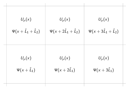
Figure 1: Valence fermions $\Psi$ living on a repeated gluon background $U_{\mu}$ with periodicity $L_{1}$, $L_{2}$ and vectors $\hat{L}_{1}=(L_{1},0)$, $\hat{L}_{2}=(0,L_{2})$.

If restricted to a finite number of QCD gauge field copies, this setup is identical to solving the Dirac operator on the repeated QCD gauge background but with QED gauge fields living in the larger volume. In the following we present a prescription to generate the infinite-volume (or large-volume) setup stochastically.

Let $\phi^{\theta}$ be a fermion field defined in finite volume with twisted boundary conditions

$$\phi^{\theta}_{x+L_{\mu}\hat{\mu}}=e^{i\theta_{\mu}}\phi^{\theta}_{x}\,,$$

where $\mu=\{x,y,z,t\}$, $L_{\mu}$ is the size of the QCD box in direction $\mu$, $\hat{\mu}$ is the unit vector in direction $\mu$, and $\theta_{\mu}$ is the twist angle in direction $\mu$. In analogy to Bloch’s theorem, the symmetry under translations by $L_{\mu}\hat{\mu}$ then yields

$$\left\langle\Psi_{x+nL}\bar{\Psi}_{y+mL}\right\rangle=\int_{0}^{2\pi}\frac{d^{4}\theta}{(2\pi)^{4}}e^{i\theta(n-m)}\left\langle\phi^{\theta}_{x}\bar{\phi}^{\theta}_{y}\right\rangle\,,$$ (1)

where the $\langle\cdot\rangle$ denotes the fermionic contraction in a fixed background gauge field $U_{\mu}(x)$, $L=\sum_{\mu}\hat{\mu}L_{\mu}$, and $x,y,n,m,\theta$ are four-vectors. For a finite number $N_{\mu}$ of QCD gauge field copies in direction $\mu$, the integral $\int_{0}^{2\pi}\frac{d\theta_{\mu}}{2\pi}$ is replaced by the sum $(1/N_{\mu})\sum_{\theta_{\mu}=0,2\pi/N_{\mu},\ldots,2\pi(N_{\mu}-1)/N_{\mu}}$. For $N_{\mu}=2$ this reduces to the well-known periodic-plus-antiperiodic trick. The twist-average of Eq. (1) may be performed stochastically and can be used to generate the infinite-volume photon momentum integrals, see Sec. 4.

The reduction of finite-volume errors through averaging of solutions with different twists is well-known in the study of metallic systems [3] but was also recently investigated in the study of two-baryon systems [4].

For a general observable, we propose the following prescription:

1. Use the infinite-volume fields $\Psi$ for all operators and sources,

2. perform the Wick contractions, and finally

3. use Eq. (1) to write the result in terms of integrals over twists involving only Dirac inversions of the finite-volume theory.

The positions of the vertices in the resulting expression can then be summed over the infinite volume. For quark-connected diagrams such a sum can be performed naïvely as described below. For quark-disconnected contributions one needs to restrict the position of separate quark loops to the same QCD box. Such a restriction can be readily implemented in the prescription discussed below.

The setup described in this section works well with multi-source methods such as AMA [5]. In the remainder of this manuscript the numerical data uses an AMA setup with only one twist vector per source (such that the number of twist vectors that are averaged coincides with the number of sources). Note that one may be able to re-use zero-twist eigenvectors by employing solvers such as [6] that use blocked eigenvectors.

3 The muon hadronic vacuum polarization

The leading-order hadronic vacuum polarization diagram, shown in Fig. 2, is conveniently evaluated following [7] which expresses the full diagram as

$$a_{\mu}=\int_{0}^{\infty}d(q^{2})F(q^{2})\hat{\Pi}(q^{2})$$ (2)

with function $F(q^{2})$ defined in [7] capturing the photon and muon components of the diagram, $\hat{\Pi}(q^{2})=\Pi(q^{2})-\Pi(0)$, $\Pi_{\mu\nu}(q)=(q_{\mu}q_{\nu}-q^{2}g_{\mu\nu})\Pi(q^{2})$. Furthermore $\Pi_{\mu\nu}(q)=\sum_{x}e^{iqx}\Pi_{\mu\nu}(x)$ and $\Pi_{\mu\nu}(x)=\left\langle V_{\mu}(x)V_{\nu}(0)\right\rangle$ with vector current $V_{\mu}$. In the following numerical examples, we use a conserved vector current at position $x$ and a local vector current at the origin.

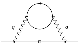
Figure 2: The leading-order hadronic vacuum polarization diagram. The lower fermion line is the muon.

Equation (2) follows the prescription that we outlined above. We couple the QCD fermion loop to an infinite-volume photon whose propagators are included in the function $F(q^{2})$. By computing $\Pi_{\mu\nu}$ defined in terms of the infinite-volume fields $\Psi$, we have access to a continuum of photon momenta $q$. The most significant simplification of this specific example is that we have reduced the four-dimensional photon momentum integral analytically to a one-dimensional integral over $q^{2}$. In this way, we can test our prescription in the case of twisting in just a single direction. In a general QCD+QED problem, we will evaluate four-dimensional photon-momentum integrals and appropriately included non-zero twist angles in all four directions.

In the remainder of this section we first explore a naïve implementation of the twist-averaging idea to evaluate $a_{\mu}$. Let $C_{\mu\nu}(t)=\sum_{\vec{x}}\Pi_{\mu\nu}(x_{0}=t,\vec{x})$, $C(t)=C_{\mu\mu}(t)$ for $\mu=x,y,z$. Then we can write down an estimator for $\hat{\Pi}(q^{2})$ that configuration-by-configuration satisfies $\hat{\Pi}(q^{2}=0)=0$ and thereby avoids a statistical noise problem for small momenta. Starting from $\left\langle\Pi_{\mu\nu}(q^{2}=0)\right\rangle=0$ and $\left\langle\operatorname{Im}\Pi_{\mu\nu}(q^{2})\right\rangle=0$ we arrive at

$$\left\langle\hat{\Pi}(q^{2})\right\rangle=\left\langle\sum_{t}\operatorname{Re}\left(\frac{\exp(iqt)-1}{q^{2}}+\frac{1}{2}t^{2}\right)\operatorname{Re}C_{\mu\mu}(t)\right\rangle$$ (3)

which is a minimal modification of Eq. (81) of [8]. This expression includes an explicit double-subtraction of $\Pi_{\mu\nu}(q^{2}=0)$ and $\Pi(q^{2}=0)$.

More specifically, we compute

averaging over independent temporal twist angles $\theta_{1}$ and $\theta_{2}$ for the two propagator lines. All spatial twists are zero such that our setup corresponds to an infinite time direction. We inject momentum only in time direction and cut the sum over time-slices at sufficiently large distance such that the contribution of the remainder can be ignored within the statistical precision. In Sec. 4, we present a method that does not require such a cut.

Figure 3 shows a numerical comparison of results using RBC/UKQCD’s $16^{3}$ and $24^{3}$ ensembles that only differ in their respective physical volume. This allows for a test of remnant finite-volume errors introduced by the sea sector. The integral over $q^{2}$ is performed using both the Trapezoidal and Simpson’s rule, choosing a step-size such that their difference is below $1/100$ of the statistical error. We find that the relative error of $a_{\mu}$ is consistent with the almost $q^{2}$-independent integrand uncertainty shown in Fig. 4.

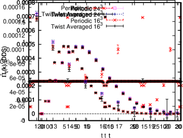
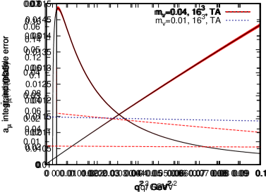
Figure 3: Strange quark contribution on RBC/UKQCD’s $16^{3}$ and $24^{3}$ ensembles with $a^{-1}\approx 1.73$ GeV, $m_{l}=0.01$ ($m_{\pi}\approx 422$ MeV), and $m_{s}=0.04$. The $16^{3}$ ($24^{3}$) measurement was performed using 2 (1) exact and 32 (16) inexact sources on 60 (78) configurations. The left figure shows the times-lice $t$ contribution to $\hat{\Pi}(k=m_{\mu})$, where $m_{\mu}$ is the physical muon mass. The right figure shows the integrand of $a_{\mu}$ as a function of $q^{2}$. Note that the stochastic noise is well-behaved for small momenta.

4 Stochastic integration of photon momenta

In this section we demonstrate an efficient method to use the twist-averaging procedure to sample over the photon momenta. A wise choice of sampling weight, i.e., the use of importance-sampling techniques can yield a substantial benefit. The following discussion is explicitly given in one dimension but all expressions and methods translate in a straightforward way to the more general four-dimensional case.

We continue the discussion of the HVP diagram to illustrate the method. The full diagram with lattice regulator can be written as

$$\int_{-\pi}^{\pi}dk\>\Gamma^{\mu\nu}(k)\Pi_{\mu\nu}(k)=\int_{-\pi}^{\pi}dk\>\Gamma^{\mu\nu}(k)\int_{0}^{2\pi}\frac{d\theta_{1}}{2\pi}\frac{d\theta_{2}}{2\pi}\sum_{x\in\{0,\ldots,L-1\},n\in\mathbbm{N}}e^{ik(nL+x)+in(\theta_{1}-\theta_{2})}C_{\mu\nu}(x,\theta_{1},\theta_{2})$$ (4)

for an appropriately defined $\Gamma^{\mu\nu}$. Poisson’s summation formula yields

$$\int_{-\pi}^{\pi}dk\>\Gamma^{\mu\nu}(k)\int_{0}^{2\pi}\frac{d\theta_{1}}{2\pi}\frac{d\theta_{2}}{2\pi}\sum_{x\in\{0,\ldots,L-1\}}e^{ikx}\hat{\delta}(k-(\theta_{2}-\theta_{1})/L)C_{\mu\nu}(x,\theta_{1},\theta_{2})$$ (5)

with $\hat{\delta}(k)=\frac{2\pi}{L}\sum_{n\in\mathbbm{N}}\delta(k+2\pi n/L)$. By writing $\int_{-\pi}^{\pi}dk\>g(k)=\frac{1}{L}\sum_{n=0,\ldots,L-1}\int_{0}^{2\pi}d\theta_{k}g(2\pi n/L+\theta_{k}/L)$ and performing the integral over $\theta_{k}$, we obtain a method to stochastically sample the photon momenta through the random choice of twist angles.

In Fig. 4 we show the resulting error for this method using the same configurations and sources as used in Fig. 3. We now, however, use importance sampling for the random twist angles such that they follow the probability distribution induced by $F(q^{2})$ of Eq. (2). We observe a slight reduction of statistical error, which may demonstrate the benefit of the importance sampling strategy.

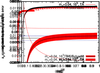
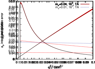
Figure 4: Relative errors of $a_{\mu}$ integrated up to maximal momentum $q^{2}$ (left) as well as the integrand of $a_{\mu}$ for $q^{2}$ (right) for the methods described in this manuscript.

The sum over $L$-translations in Eq. (4) generates conservation of the small-momentum component $\theta_{k}=\theta_{2}-\theta_{1}$. This leads to an intuitive pictorial prescription in momentum space

with average over twist-angle $\theta_{q}$ and sum over finite-volume periodic momenta $q_{\rm PBC}$.

5 QED mass splittings

A potentially interesting application of the ideas explained above is the computation of QED mass splittings. For a general meson two point function, one needs to evaluate (ignoring quark-disconnected diagrams for now)

$=C_{0}(t)+\alpha C_{1}(t)$

for which the mass-shifts could be obtained from effective mass plots following

$$m_{\rm eff}(t)=m_{\rm eff,0}(t)+\alpha m_{\rm eff,1}(t)\,,\qquad m_{\rm eff,1}(t)=\frac{C_{1}(t)}{C_{0}(t)}-\frac{C_{1}(t+1)}{C_{0}(t+1)}\,.$$

In this general case a four-dimensional photon momentum integral and hence a four-dimensional twist-averaging procedure is necessary. Using an appropriate importance-sampling of twist angles, the methods outlined above should be applicable in a straightforward manner. The photon propagator could, e.g., be implemented stochastically in a sequential source setup.

For a first test that allows us to re-use the HVP measurements, we use current algebra and soft pion theorems [9] and compute

.

Results of a quick numerical test are shown in Fig. 5.

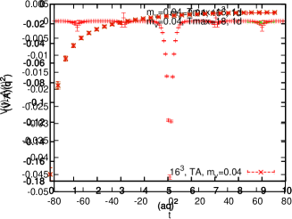
Figure 5: V-A contribution for the strange quark loop. At large $q^{2}$ there is a gap due to the heavy mass such that the integral does not converge. The stochastic integration method of the photon momentum with $(aq)^{2}<1$ cut yields an $\approx 4\%$ statistical error.

6 Conclusion

We have proposed a prescription to put valence fermions and photons in infinite volume. We expect a substantial reduction of finite-volume errors in lattice QCD+QED simulations in this setup such that regular lattice QCD boxes could be used for combined QCD+QED simulations. We have discussed both a naïve implementation of the idea and a refined strategy that samples over photon momenta stochastically. In the latter method an importance-sampling strategy seems promising.

In the future, the methods presented here will be tested for realistic pion masses in the context of QED mass splittings, QED corrections to decay constants, as well as finite-volume corrections to the hadronic contributions to $(g-2)_{\mu}$, in particular the light-by-light contribution.

Acknowledgements We thank our colleagues of the RBC and UKQCD collaborations and in particular Tom Blum, Norman Christ, Luchang Jin, and Chulwoo Jung for fruitful discussions. T.I and C.L are supported in part by US DOE Contract #AC-02-98CH10886(BNL). T.I is also supported by Grants-in-Aid for Scientific Research #26400261.

References

- [1] S. Borsanyi, S. Durr, Z. Fodor, C. Hoelbling, and S. D. Katz et al., arXiv:1406.4088 [hep-lat].
- [2] Z. Davoudi and M. J. Savage, Phys. Rev. D 90, no. 5, 054503 (2014) [arXiv:1402.6741 [hep-lat]].
- [3] C. Lin, F.-H. Zong, and D. M. Ceperley, Phys. Rev. E 64, 016702 (2001) [arXiv:cond-mat/0101339]; Loh and Campbell 1988 E. Y. Loh Jr. and D. K. Campbell, Synth. Metals 27, A499 (1988).
- [4] R. A. Briceno, Z. Davoudi, T. C. Luu and M. J. Savage, Phys. Rev. D 89, no. 7, 074509 (2014) [arXiv:1311.7686 [hep-lat]].
- [5] T. Blum, T. Izubuchi and E. Shintani, Phys. Rev. D 88, no. 9, 094503 (2013) [arXiv:1208.4349 [hep-lat]]; E. Shintani, R. Arthur, T. Blum, T. Izubuchi, C. Jung, and C. Lehner, arXiv:1402.0244 [hep-lat].
- [6] P. A. Boyle, arXiv:1402.2585 [hep-lat].
- [7] T. Blum, Phys. Rev. Lett. 91, 052001 (2003) [hep-lat/0212018].
- [8] D. Bernecker and H. B. Meyer, Eur. Phys. J. A 47, 148 (2011) [arXiv:1107.4388 [hep-lat]].
- [9] T. Das, G. S. Guralnik, V. S. Mathur, F. E. Low and J. E. Young, Phys. Rev. Lett. 18, 759 (1967); E. Shintani et al. [JLQCD Collaboration], PoS LAT 2007, 134 (2007) [arXiv:0710.0691 [hep-lat]].