High-field magnetoconductivity of topological semimetals with short-range potential

Abstract

Weyl semimetals are three-dimensional topological states of matter, in a sense that they host paired monopoles and antimonopoles of Berry curvature in momentum space, leading to the chiral anomaly. The chiral anomaly has long been believed to give a positive magnetoconductivity or negative magnetoresistivity in strong and parallel fields. However, several recent experiments on both Weyl and Dirac topological semimetals show a negative magnetoconductivity in high fields. Here, we study the magnetoconductivity of Weyl and Dirac semimetals in the presence of short-range scattering potentials. In a strong magnetic field applied along the direction that connects two Weyl nodes, we find that the conductivity along the field direction is determined by the Fermi velocity, instead of by the Landau degeneracy. We identify three scenarios in which the high-field magnetoconductivity is negative. Our findings show that the high-field positive magnetoconductivity may not be a compelling signature of the chiral anomaly and will be helpful for interpreting the inconsistency in the recent experiments and earlier theories.

I Introduction

Topological semimetals are three-dimensional topological states of matter. Their band structures look like three-dimensional analogue of graphene, in which the conduction and valence energy bands with linear dispersions touch at a finite number of points, i.e., Weyl nodes Balents (2011). The nodes always occur in pairs and carry opposite chirality. One of the topological aspects of Weyl semimetals is that they host pairs of monopole and anti-monopole of Berry curvature in momentum space Volovik (2003); Wan et al. (2011) (see Fig. 1), and the fluxes of Berry curvature flow from one monopole to the other. In the presence of both a magnetic field and an electric field along the direction that connects two monopoles, electrons can be pumped from one monopole to the other, leading to the Adler-Bell-Jackiw chiral anomaly Adler (1969); Bell and Jackiw (1969); Nielsen and Ninomiya (1981) (also known as triangle anomaly). Recently, angle-resolved photoemission spectroscopy (ARPES) has identified the Dirac nodes Young et al. (2012) (doubly-degenerate Weyl nodes) in (Bi_1-xIn_x)₂Se₃ Brahlek et al. (2012); Wu et al. (2013), Na₃Bi Wang et al. (2012); Liu et al. (2014a); Wang et al. (2013); Xu et al. (2015), and Cd₃As₂ Wang et al. (2013); Liu et al. (2014b); Neupane et al. (2014); Yi et al. (2014); Borisenko et al. (2014) and Weyl nodes in TaAs Weng et al. (2015); Huang et al. (2015a); Lv et al. (2015); Xu et al. . Also, scanning tunneling microscopy has observed the Landau quantization in Cd₃As₂ Jeon et al. (2014) and TlBiSSe Novak et al. (2014).

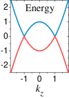
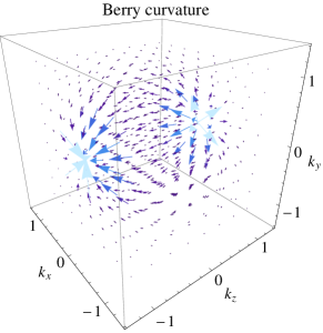
Figure 1: Left: the energy spectrum of a Weyl semimetal as a function of $k_{z}$ at $k_{x}=k_{y}=0$. Right: the vector plot of the Berry curvature of a Weyl semimetal. $(k_{x},k_{y},k_{z})$ is the wave vector. The analytic expression of the three-dimensional Berry curvature is given in Eq. (3). The parameters are $M_{0}=M_{1}=A=1$, so $k_{c}=1$.

While the chiral anomaly is well established in momentum space, it becomes a challenging issue how to detect the effects of the chiral anomaly or relevant physical consequences. This has been attracting a lot of theoretical efforts, such as the prediction of negative parallel magnetoresistance Nielsen and Ninomiya (1983); Aji (2012); Son and Spivak (2013); Burkov (2014a), proposal of non-local transport Parameswaran et al. (2014), using electronic circuits Kharzeev and Yee (2013), plasmon mode Zhou et al. (2015), etc. In particular, whether or not the chiral anomaly could produce measurable magnetoconductivity is one of the focuses in recent efforts. This has inspired a number of transport experiments in topological semimetals Cd₃As₂ Liang et al. (2015); Feng et al. (2014); He et al. (2014); Zhao et al. (2014); Cao et al. (2014); Narayanan et al. (2015), ZrTe₅ Li et al. (2014), NbP Shekhar et al. (2015), Na₃Bi Xiong et al. (2015), and TaAs Huang et al. (2015b); Zhang et al. (2015). The chiral anomaly has been claimed to be verified in several different topological semimetals, including BiSb alloy Kim et al. (2013), ZrTe₅ Li et al. (2014), TaAs Huang et al. (2015b); Zhang et al. (2015), and Na₃Bi Xiong et al. (2015), in which similar magnetoconductivity behaviors are observed when the magnetic field is applied along the conductivity measurement direction: (i) In weak fields, a $-\sqrt{B}$ negative magnetoconductivity is observed at low temperatures, consistent with the quantum transport theory of the weak antilocalization of Weyl or Dirac fermions in three dimensions Kim et al. (2013); Lu and Shen (2014). (ii) In intermediate fields, a $B^{2}$ positive magnetoconductivity is observed, as expected by the theory of the semiclassical conductivity arising from the chiral anomaly Son and Spivak (2013); Ramakrishnan et al. (2015); Burkov (2014a). (iii) In high fields, the magnetoconductivity is always negative in the experiments. However, in the strong-field limit, a positive magnetoconductivity is expected in existing theories, also as one of the signatures of the chiral anomaly Nielsen and Ninomiya (1983); Aji (2012); Son and Spivak (2013); Gorbar et al. (2014).

In this work, we focus on the high-field limit, and present a systematic calculation on the conductivity of topological semimetals. Beyond the previous treatments, we start with a two-node model that describes a pair of Weyl nodes with a finite distance in momentum space. Moreover, we fully consider the magnetic field dependence of the scattering time for electrons on each Landau level, and obtain a conductivity formula. The efforts lead to qualitatively distinct results compared to all the previous theories. We find that the conductivity does not grow with the Landau degeneracy but mainly depends on the Fermi velocity. The magnetoconductivity arises from the field dependence of the Fermi velocity when the chemical potential is tuned by the magnetic field. Based on this formula and the model, we find that although the positive magnetoconductivity is also possible, three cases can be identified in which the magnetoconductivity is negative, possibly applicable to those observed in the experiments in high magnetic fields.

The paper is organized as follows. In Sec. II, we introduce the two-node model and show how it carries all the topological properties of a topological semimetal. In Sec. III, we present the solutions of the Landau bands of the semimetal in a magnetic field applied along the $z$ direction (the two Weyl nodes are separated along this direction). In Sec. IV, we calculate the $z$-direction magnetoconductivity in the presence of the short-range delta scattering potential. In Sec. V, we discuss various scenarios that the negative or positive magnetoconductivity may occur. In Sec. VI, we present the transport in the $x-y$ plane, including the $x$-direction conductivity and the Hall conductance. Finally, a summary of three scenarios of the negative magnetoconductivity is given in Sec. VII. The details of the calculations are provided in Appendices A-D.

II Model and its topology

A minimal model for a Weyl semimetal is

$$H=A(k_{x}\sigma_{x}+k_{y}\sigma_{y})+\mathcal{M_{\mathbf{k}}}\sigma_{z},$$ (1)

where $\sigma$ are the Pauli matrices, $\mathcal{M}_{\mathbf{k}}=M_{0}-M_{1}(k_{x}^{2}+k_{y}^{2}+k_{z}^{2})$, $(k_{x},k_{y},k_{z})$ is the wave vector, and $A$, $M_{0/1}$ are model parameters. This minimal model gives a global description of a pair of Weyl nodes of opposite chirality and all the topological properties. It has an identical structure as that for A-phase of ³He superfluids Shen (2012) The dispersions of two energy bands of this model are $E_{\pm}=\pm\sqrt{\mathcal{M}_{\mathbf{k}}^{2}+A^{2}(k_{x}^{2}+k_{y}^{2})}$, which reduce to $E_{\pm}=\pm|M_{0}-M_{1}k_{z}^{2}|$ at $k_{x}=k_{y}=0$. If $M_{0}M_{1}>0$, the two bands intersect at $(0,0,\pm k_{c})$ with $k_{c}\equiv\sqrt{M_{0}/M_{1}}$ (see Fig. 1). Around the two nodes $(0,0,\pm k_{c})$, $H$ reduces to two separate local models

$$H_{\pm}=\mathbf{M}_{\pm}\cdot\sigma,$$ (2)

$H_{\pm}=\mathbf{M}_{\pm}\cdot\sigma$with $\mathbf{M}_{\pm}=\left(A\widetilde{k}_{x},A\widetilde{k}_{y},\mp 2M_{1}k_{c}\widetilde{k}_{z}\right)$ and $(\widetilde{k}_{x},\widetilde{k}_{y},\widetilde{k}_{z})$ the effective wave vector measured from the Weyl nodes.

The topological properties in $H$ can be seen from the Berry curvature Xiao et al. (2010), $\Omega(\mathbf{k})$ = $\nabla_{\mathbf{k}}\times\mathbf{A}(\mathbf{k})$, where the Berry connection is defined as $\mathbf{A}(\mathbf{k})$ = $i\left\langle u(\mathbf{k})\right|\nabla_{\mathbf{k}}\left|u(\mathbf{k})\right\rangle$. For example, for the energy eigenstates for the $+$ band $\left|u(\mathbf{k})\right\rangle$ = $[\cos(\Theta/2),\sin(\Theta/2)e^{i\varphi}]$, where $\cos\Theta\equiv\mathcal{M}_{\mathbf{k}}/E_{+}$ and $\tan\varphi\equiv k_{y}/k_{x}$. The three-dimensional Berry curvature for the two-node model can be expressed as

$$\boldsymbol{\Omega}\left(\mathbf{k}\right)=\frac{A^{2}M_{1}}{E_{+}^{3}}\left[k_{z}k_{x},k_{z}k_{y},\frac{1}{2}\left(k_{z}^{2}-k_{c}^{2}-k_{x}^{2}-k_{y}^{2}\right)\right].$$ (3)

When $M_{0}M_{1}>0$, there exist a pair of singularities at $(0,0,\pm k_{c})$ as shown in Fig. 1. The chirality of a Weyl node can be found as an integral over the Fermi surface enclosing one Weyl node $(1/2\pi)\oint\Omega(\mathbf{k})\cdot d\mathbf{S(\mathbf{k})}$, which yields opposite topological charges $\mp\mathrm{sgn}(M_{1})$ at $\pm k_{c}$, corresponding to a pair of “magnetic monopole and antimonopole” in momentum space. For a given $k_{z}$, a Chern number can be well defined as $n_{c}(k_{z})=-(1/2\pi)\iint dk_{x}dk_{y}\Omega(\mathbf{k})\cdot\hat{z}$ to characterize the topological property in the $k_{x}$-$k_{y}$ plane, and $n_{c}(k_{z})=-\frac{1}{2}[\mathrm{sgn}(M_{0}-M_{1}k_{z}^{2})+\mathrm{sgn}(M_{1})]$ Lu et al. (2010). For $M_{0}M_{1}>0$, $n_{c}(k_{z})=-\mathrm{sgn}(M_{1})$ for $-k_{c}<k_{z}<k_{c}$, and $n_{c}(k_{z})=0$ for other cases Yang et al. (2011). The nonzero Chern number corresponds to the $k_{z}$-dependent edge states (known as the Fermi arc) according to the bulk-boundary correspondence Hatsugai (1993). Thus the two-node model in Eq. (1) provides a generic description for Weyl semimetals, including the band touching, opposite chirality, monopoles of Berry curvature, topological charges, and Fermi arc. In the following we shall focus on the topological case of $M_{0}M_{1}>0$.

III Landau bands

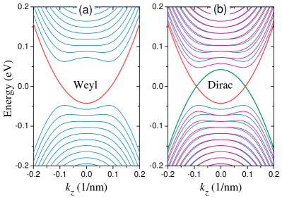
Figure 2: The energies of Landau bands of the minimal global model for Weyl and Dirac semimetals in a magnetic field $B$ applied along the $z$ direction, as functions of the wave vector $k_{z}$. The parameters: $M_{0}=0.05$ eV, $M_{1}=5$ eV$\cdot$nm², $A=1$ eV$\cdot$nm, and $B=1$ Tesla. The Zeeman energy is not included.

In a magnetic field along the $z$ direction, the energy spectrum is quantized into a set of 1D Landau bands dispersing with $k_{z}$ [see Fig. 2 (a)]. We consider a magnetic field applied along the $z$ direction, $\mathbf{B}=(0,0,B)$, and choose the Landau gauge in which the vector potential is $\mathbf{A}=(-yB,0,0)$. Under the Pierls replacement, the wave vector in the Hamiltonian in Eq. (1) is replaced by the operator

$$\mathbf{k}=(k_{x}-\frac{eB_{z}}{\hbar}y,-i\partial_{y},k_{z})$$ (4)

$k_{x}$ and $k_{z}$ are still the good quantum numbers as the introduction of the gauge field does not break the translational symmetry along the x and z direction. Introducing the ladder operators Shen et al. (2004, 2005), $k_{x}^{2}+k_{y}^{2}\rightarrow\omega(a^{{\dagger}}a+1/2)$, $k_{+}\rightarrow(\sqrt{2}/\ell_{B})a^{{\dagger}}$, $k_{-}\rightarrow(\sqrt{2}/\ell_{B})a$, where the magnetic length $\ell_{B}=\sqrt{\hbar/eB}$ and the ladder operators $a\equiv-[(y-\ell_{B}^{2}k_{x})/\ell_{B}+\ell_{B}\partial_{y}]/\sqrt{2}$ and $a^{{\dagger}}\equiv-[(y-\ell_{B}^{2}k_{x})/\ell_{B}-\ell_{B}\partial_{y}]/\sqrt{2}$ Sakurai (1993); Shen et al. (2004), then we can write the Hamiltonian in terms of the ladder operators,

$$H(\mathbf{k})=\left[\begin{array}[]{cc}M_{k}&Ak_{-}\\ Ak_{+}&-M_{k}\end{array}\right]\rightarrow\left[\begin{array}[]{cc}M_{a}&\eta a\\ \eta a^{{\dagger}}&-M_{a}\end{array}\right],$$ (9)

where $\mathcal{M}_{a}=M_{0}-M_{1}k_{z}^{2}-\omega(a^{{\dagger}}a+1/2)$, $\omega=2M_{1}/\ell_{B}^{2}$, and $\eta=\sqrt{2}A/\ell_{B}$. With the trial wave functions $(c_{1}|\nu-1\rangle,c_{2}|\nu\rangle)^{T}$ for $\nu=1,2,...$ (later denoted as $\nu\geq 1$) and $(0,|0\rangle)^{T}$ for $\nu=0$, where $\nu$ indexes the Hermite polynomials, the eigen energies $E$ can be found from the secular equation

$$\det\left[\begin{array}[]{cc}\mathcal{M}_{\nu}+\omega/2-E&\eta\sqrt{\nu}\\ \eta\sqrt{\nu}&-\mathcal{M}_{\nu}+\omega/2-E\end{array}\right]=0$$ (10)

for $\nu\geq 1$, and $-\mathcal{M}_{\nu}+\omega/2-E=0$ for $\nu=0$, where $\mathcal{M}_{\nu}=M_{0}-M_{1}k_{z}^{2}-\omega\nu$. The eigen energies are

$$E_{k_{z}}^{\nu\pm} = \omega/2\pm\sqrt{\mathcal{M}_{\nu}^{2}+\nu\eta^{2}},\ \nu\geq 1$$

$$E_{k_{z}}^{0} = \omega/2-M_{0}+M_{1}k_{z}^{2},\ \ \nu=0.$$ (11)

This represents a set of Landau energy bands ($\nu$ as band index) dispersing with $k_{z}$, as shown in Fig. 2. The eigen states for $\nu\geq 1$ are

$$|\nu\geq 1,k_{x},k_{z},+\rangle = \left[\begin{array}[]{cc}\cos\frac{\theta_{k_{z}}^{\nu}}{2}|\nu-1\rangle\\ \sin\frac{\theta_{k_{z}}^{\nu}}{2}|\nu\rangle\end{array}\right]|k_{x},k_{z}\rangle,$$ (14)

$$|\nu\geq 1,k_{x},k_{z},-\rangle = \left[\begin{array}[]{cc}\sin\frac{\theta_{k_{z}}^{\nu}}{2}|\nu-1\rangle\\ -\cos\frac{\theta_{k_{z}}^{\nu}}{2}|\nu\rangle\end{array}\right]|k_{x},k_{z}\rangle,$$ (17)

and for $\nu=0$ is

$$|\nu=0,k_{x},k_{z}\rangle=\left[\begin{array}[]{cc}0\\ |0\rangle\end{array}\right]|k_{x},k_{z}\rangle,$$ (18)

where $\cos\theta=\mathcal{M}_{\nu}/\sqrt{\mathcal{M}_{\nu}^{2}+\nu\eta^{2}}$, and the wave functions $\psi_{\nu,k_{z},k_{x}}(\mathbf{r})=\langle\mathbf{r}|\nu,k_{x},k_{z}\rangle$ are found as

$$\psi_{\nu,k_{z},k_{x}}(\mathbf{r}) = \frac{C_{\nu}}{\sqrt{L_{x}L_{z}\ell_{B}}}e^{ik_{z}z}e^{ik_{x}x}e^{-\frac{(y-y_{0})^{2}}{2\ell_{B}^{2}}}\mathcal{H}_{\nu}(\frac{y-y_{0}}{\ell_{B}}),$$

where $C_{\nu}\equiv 1/\sqrt{\nu!2^{\nu}\sqrt{\pi}}$, $L_{x}L_{z}$ is area of sample, the guiding center $y_{0}=k_{x}\ell_{B}^{2}$, $\mathcal{H}_{\nu}$ are the Hermite polynomials. As the dispersions are not explicit functions of $k_{x}$, the number of different $k_{x}$ represents the Landau degeneracy $N_{L}=1/2\pi\ell_{B}^{2}=eB/h$ in a unit area in the x-y plane.

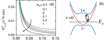
Figure 4: (a) The $x$-direction conductivity of the 0-th Landau band of the Weyl semimetal as a function of the $z$ direction magnetic field $B$, for different values of the carrier density $n_{0}$ (in units of $10^{17}$/cm³). (b) Schematic of the second-order processes that contribute to the $x$ direction conductivity. Parameters: $M_{0}=0.05$ eV, $M_{1}=5$ eV$\cdot$nm², $A=1$ eV$\cdot$nm, $V_{\text{imp}}=10$ (eV)²$\cdot$nm³.

This set of analytical solutions provides us a good base to study the transport properties of Weyl fermions. In the following, we will focus on the quantum limit, i.e., only the $\nu=0$ band is on the Fermi surface [see Fig. 4 (b)].

IV z-direction semiclassical conductivity

IV.1 Argument of positive magnetoconductivity

When the Fermi energy is located between the two states of $|\nu=1,k_{x},k_{z},\pm\rangle$, all the bands for $|\nu\geq 1,k_{x},k_{z},+\rangle$ are empty and all the bands $|\nu\geq 1,k_{x},k_{z},-\rangle$ are fully occupied. Only the band of $\nu=0$ is partially filled. In this case the transport properties of the system are dominantly determined by the highly degenerate $\nu=0$ Landau bands [the red curve in Fig. 2 (a)] . It is reasonable to regard them as a bundle of one-dimensional chains. Combining the Landau degeneracy $N_{L}$, the $z$-direction conductance is approximately given by

$$\sigma_{zz}=N_{L}\sigma_{\text{1D}},$$ (20)

where $\sigma_{\text{1D}}$ is the conductance for each one-dimensional Landau band.

If we ignore the scattering between the states in the degenerate Landau bands, according to the transport theory, the ballistic conductance of a one-dimensional chain in the clean limit is given by

$$\sigma_{\text{1D}}=\frac{e^{2}}{h},$$ (21)

then the conductivity is found as

$$\sigma_{zz}=\frac{e^{2}}{h}\frac{eB}{h},$$ (22)

which is is linear in magnetic field $B$, giving a positive magnetoconductivity.

In most measurements, the sample size is much larger than the mean free path, then the scattering between the states in the Landau bands is inevitable, and we have to consider the other limit, i.e., the diffusive limit. Usually, the scattering is characterized by a momentum relaxation time $\tau$. According to the Einstein relation, the conductivity of each Landau band in the diffusive limit is

$$\sigma_{\text{1D}}=e^{2}N_{\text{1D}}v_{F}^{2}\tau,$$ (23)

where $v_{F}$ the Fermi velocity and the density of states for each 1D Landau band is $N_{\text{1D}}=1/\pi\hbar v_{F}$, then

$$\sigma_{zz}=\frac{e^{2}}{h}\frac{eBv_{F}\tau}{\pi\hbar}.$$ (24)

If $v_{F}$ and $\tau$ are constant, one readily concludes that the magnetoconductivity is positive and linear in $B$.

According to Nielsen and Ninomiya Nielsen and Ninomiya (1983), to illustrate the physical picture of the chiral anomaly, they started with a one-dimensional model in which two chiral energy bands have linear dispersions and opposite velocities. An external electric field can accelerate electrons in one band to higher energy levels, in this way, charges are “created”. In contrast, in the other band, which has the opposite velocity, charges are annihilated. The chiral charge, defined as the difference between the charges in the two bands, therefore is not conserved in the electric field. This is literally the chiral anomaly. As one of the possible realizations of the one-dimensional chiral system, they then proposed to use the $\nu=0$ Landau bands of a three-dimensional semimetal, and expected “the longitudinal magneto-conduction becomes extremely strong”. In other words, the magnetoresistance of the 0th Landau bands in semimetals is the first physical quantity that was proposed as one of the signatures of the chiral anomaly.

Recently, several theoretical works have formulated the negative magnetoresistance or positive magnetoconductivity in the quantum limit as one of the signatures of the chiral anomaly Son and Spivak (2013); Gorbar et al. (2014), much similar to those in Eqs. (22) and (24). In both cases, the positive magnetoconductivity arises because the Landau degeneracy increases linearly with $B$. However, in the following, we will show that if $v_{F}$ and $\tau$ also depend on the magnetic field, the conclusion has to be reexamined.

IV.2 Green function calculation

Now we are ready to present the conductivity in the presence of the magnetic field when the Fermi energy is located near the Weyl nodes. The temperature is assumed to be much lower than the gap between bands $1+$ and $1-$, i.e, $k_{B}T\ll 2\sqrt{2}A/\ell_{B}$. In this case all the Landau levels of $E_{k_{z}}^{\nu-}$ are fully occupied while the $\nu=0$ band [the red curve in Fig. 2 (a)] is partially filled. Since $E_{k_{z}}^{0}$ is only a function of $k_{z}$, and independent of $k_{x}$, the system can be regarded as a bundle of highly degenerate one-dimensional chains. Along the $z$ direction, the semiclassical Drude conductivity can be found from the formula Datta (1997)

$$\sigma_{zz,0}^{sc}=\frac{e^{2}\hbar}{2\pi V}\sum_{k_{z},k_{x}}(v_{0}^{z})^{2}G_{0}^{R}G_{0}^{A},$$ (25)

where $-e$ is the electron charge, $V=L_{x}L_{y}L_{z}$ is the volume with $L_{x}$ the length along the $x$ direction and so on, $v_{0}^{z}=\partial E_{k_{z}}^{0}/\hbar\partial k_{z}=2M_{1}k_{z}/\hbar$ is the velocity along the $z$ direction for a state with wave vector $k_{z}$ in the $\nu=0$ band, $G_{0}^{R/A}=1/(E_{F}-E_{k_{z}}^{0}\pm i\hbar/2\tau^{0})$ is the retarded/advanced Green’s function, with $\tau^{0}$ the lifetime of a state in the $\nu=0$ band with wave vector $k_{x}$ and $k_{z}$. Usually, in the diffusive regime, one can replace $G_{0k_{z}}^{R}G_{0k_{z}}^{A}$ by $\frac{2\pi}{\hbar}\tau_{k_{x}}^{0}\delta(E_{F}-E_{k_{z}}^{0})$. However, in one dimension, to correct the van Hove singularity at the band edge, we introduce an extra correction factor $\Lambda$, so that $G_{0k_{z}}^{R}G_{0k_{z}}^{A}=\frac{2\pi}{\hbar}\Lambda\tau_{k_{x}}^{0}\delta(E_{F}-E_{k_{z}}^{0})$. As shown in Appendix A, $\Lambda\rightarrow 1$ (0) if the Fermi energy is far away from (approaching) the band edge. Now the conductivity formula can be written as

$$\sigma_{zz,0}^{sc} = \frac{e^{2}\hbar}{2\pi V}\sum_{k_{z},k_{x}}(v_{0k_{z}}^{z})^{2}\frac{2\pi}{\hbar}\Lambda\tau_{k_{x}}^{0}\delta(E_{F}-E_{k_{z}}^{0}).$$ (26)

The delta function $\delta(E_{F}-E_{k_{z}}^{0})=2\frac{\delta(k_{F}^{0}-k_{z})}{\hbar|v_{F}^{0}|}$, where $v_{F}^{0}=2|M_{1}|k_{F}^{0}/\hbar$ is the absolute value of the Fermi velocity of the $\nu=0$ band with $k_{F}^{0}$ the Fermi wave vector. This allows us to perform the summation over $k_{z}$, then

$$\sigma_{zz,0}^{sc} = \frac{e^{2}}{h}\frac{2v_{F}^{0}}{L_{x}L_{y}}\sum_{k_{x}}\Lambda\tau_{k_{x}}^{0}.$$ (27)

The summation over $k_{x}$ is limited by the Landau degeneracy, finally we can reduce the conductivity formula to

$$\sigma_{zz,0}^{sc} = \frac{e^{2}}{h}\frac{v_{F}^{0}}{\pi L_{y}}\int_{-L_{y}/2\ell_{B}^{2}}^{L_{y}/2\ell_{B}^{2}}dk_{x}\tau^{0}\Lambda.$$ (28)

The scattering time $\tau^{0}$ depends on the wave packet of the Landau levels in band 0 and is a function of magnetic field. It can be found from the iteration equation under the self-consistent Born approximation (see Appendix B for details)

$$\hbar/2\tau^{0}=\sum_{k_{x}^{\prime},k_{z}^{\prime}}\frac{\langle|U_{k_{x}k_{z},k_{x}^{\prime}k_{z}^{\prime}}^{0,0}|^{2}\rangle(\hbar/2\tau^{0})}{[(E_{F}-E_{k_{z}}^{0})^{2}+(\hbar/2\tau^{0})^{2}]},$$ (29)

where $U_{k_{x}k_{z},k_{x}^{\prime}k_{z}^{\prime}}^{0,0}$ represents the scattering matrix elements, $\langle...\rangle$ means the average over impurity configurations. The conductivity in semimetals in vanishing magnetic field has been discussed within the Born approximation Das Sarma and Hwang (2015).

In this work, we consider only the short-range delta scattering potential. The delta potential takes the form

$$U(\mathbf{r})=\sum_{i}u_{i}\delta(\mathbf{r}-\mathbf{R}_{i}),$$ (30)

where $u_{i}$ measures the strength of scattering for an impurity at $\mathbf{R}_{i}$, and the potential is delta correlated $\left\langle U\left(\mathbf{r}\right)U\left(\mathbf{r}^{\prime}\right)\right\rangle=V_{\text{imp}}\delta(\mathbf{r}-\mathbf{r}^{\prime})$, where $V_{\text{imp}}$ is a field-independent parameter that is proportional to the impurity density and averaged field-independent scattering strength. Using the wave function of the $\nu=\text{0}$ band, we find that (see Appendix C)

$$\langle|U_{k_{x}k_{z},k_{x}^{\prime}k_{z}^{\prime}}^{0,0}|^{2}\rangle=\frac{V_{\text{imp}}\exp[-\ell_{B}^{2}(k_{x}-k_{x}^{\prime})^{2}/2]}{L_{x}L_{z}\ell_{B}\sqrt{2\pi}},$$ (31)

and in the strong-field limit ($B\rightarrow\infty$),

$$\tau^{0}\Lambda = \frac{\hbar^{2}v_{F}^{0}\pi\ell_{B}^{2}}{V_{\text{imp}}},$$ (32)

which gives the conductivity in the strong-field limit as

$$\sigma_{zz,0}^{sc} = \frac{e^{2}}{h}\frac{(\hbar v_{F}^{0})^{2}}{V_{\text{imp}}}.$$ (33)

Notice that the Landau degeneracy in the scattering time cancels with that in Eq. (28), thus the magnetic field dependence of $\sigma_{zz,0}^{sc}$ is given by the Fermi velocity $v_{F}^{0}$. This is one of the main results in this paper. When ignoring the magnetic field dependence of the Fermi velocity, a $B$-independent conductivity was concluded, which is consistent with the previous work in which the velocity is constant Aji (2012). Later, we will see the magnetic field dependence of the Fermi velocity can lead to different scenarios of positive and negative magnetoconductivity.

V Scenarios of negative and positive z-direction magnetoconductivity

V.1 Weyl semimetal with fixed carrier density

In a strong field the Fermi velocity or the Fermi energy is given by the density of charge carriers and the magnetic field Abrikosov (1998). We assume that an ideal Weyl semimetal is the case that the Fermi energy crosses the Weyl nodes, all negative bands are fully filled and the positive bands are empty. In this case $\hbar v_{F}^{0}=2M_{1}k_{c}$. An extra doping of charge carriers will cause a change of electron density $n_{0}(>0)$ in the electron-doped case or hole density $n_{0}(<0)$ in the hole-doped case. The relation between the Fermi wave vector and the density of charge carriers is given by

$$n_{0}=2N_{L}\times\frac{k_{F}^{0}-k_{c}}{2\pi}$$ (34)

This means that the Fermi wave vector is determined by the density of charge carriers $n_{0}$ and magnetic field $B$,

$$k_{F}^{0} = k_{c}+\pi n_{0}h/eB$$ (35)

or $k_{F}^{0}=k_{c}+2\pi^{2}n_{0}\ell_{B}^{2}$. Thus the Fermi velocity is also a function of B, $\hbar v_{F}^{0}=2M_{1}k_{F}^{0},$ and

$$\sigma_{zz,0}^{sc}=\sigma_{N}\left[1+\mathrm{sgn}(n_{0})\frac{B_{c}}{B}\right]^{2}.$$ (36)

where the characteristic field $B_{c}=\pi\left|n_{0}\right|h/ek_{c}$. A typical order of $B_{c}$ is about 10 Tesla for $n_{0}$ of 10¹⁷/cm³ [see Fig. 3 (b)]. $\sigma_{zz,0}^{sc}$ is constant for the undoped case of $n_{0}=0$, and

$$\sigma_{N}=\frac{e^{2}}{h}\frac{4M_{1}^{2}k_{c}^{2}}{V_{\text{imp}}}$$ (37)

is the conductivity of the undoped case, and is independent of magnetic field. Thus the magnetoconductivity is always negative in the electron-doped case while always positive in the hole-doped regime as shown in Fig. 3 (a).

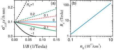
Figure 3: (a) The $z$-direction conductivity of the 0-th Landau band of the Weyl semimetal as a function of the $z$ direction magnetic field $B$, for different values of the carrier density $n_{0}$ (in units of $10^{17}$/cm³). The lower bound of the field for each curve is determined by the bottom of band $1+$ for $n_{0}>0$ or the bottom of band 0 for $n_{0}<0$. (b) The characteristic $B_{c}$ defined in Eq. (36) as a function of $n_{0}$. Parameters: $M_{0}=0.05$ eV, $M_{1}=5$ eV$\cdot$nm², $A=1$ eV$\cdot$nm, $V_{\text{imp}}=10$ (eV)²$\cdot$nm³. Using $n_{0}=(8\pi/3)E_{F}^{3}/2M_{1}k_{c}A^{2}(2\pi)^{3}$, a carrier density of $n_{0}\times 10^{17}$/cm³corresponds to a Fermi energy of about $E_{F}=$144$\times{}^{3}\sqrt{n_{0}}$ meV.

V.2 Weyl semimetal with fixed Fermi energy

In the case that the Fermi energy is fixed, $(\hbar v_{F}^{0})^{2}=4M_{1}(E_{F}-eM_{1}B/\hbar+M_{0})$, and we have

$$\sigma_{zz,0}^{sc} = \frac{e^{2}}{h}\frac{4M_{1}(E_{F}-eM_{1}B/\hbar+M_{0})}{V_{\text{imp}}},$$ (38)

then the magnetoconductivity is always negative and linear in $B$.

V.3 Dirac semimetal

If the system has time-reversal symmetry, we may have a Dirac semimetal, instead of Weyl semimetal, and all Weyl nodes turn to doubly-degenerate Dirac nodes. A model for Dirac semimetal can be constructed Wang et al. (2013) by adding a time-reversal partner to Eq. (1)

$$H_{\text{Dirac}}=\left[\begin{array}[]{cc}H(\mathbf{k})&0\\ 0&H^{*}(-\mathbf{k})\end{array}\right]+\sigma_{z}\otimes\left[\begin{array}[]{cc}\Delta_{s}&0\\ 0&\Delta_{p}\end{array}\right].$$ (39)

In the second term, the $z$-direction Zeeman energy $\Delta_{s/p}=g_{s/p}\mu_{B}B/2$ is also included, where $g_{s/p}$ is the g-factor for the $s/p$ orbital Jeon et al. (2014) and $\mu_{B}$ is the Bohr magneton. Fig. 2 (b) shows the Landau bands of both $H(\mathbf{k})$ and $H^{*}(-\mathbf{k})$ in the $z$-direction magnetic field. The Landau bands of the Dirac semimetal can be found in a similar way as that in Sec. III. Now there are two branches of $\nu=0$ bands, with the energy dispersions $E_{k_{z}}^{0\uparrow}=\omega/2+\Delta_{p}-M_{0}+M_{1}k_{z}^{2}$ and $E_{k_{z}}^{0\downarrow}=-\omega/2-\Delta_{s}+M_{0}-M_{1}k_{z}^{2}$ for $H(\mathbf{k})$ and $H^{*}(-\mathbf{k})$, respectively. They intersect at $k_{z}=\pm\sqrt{[M_{0}-(\omega+\Delta_{s}+\Delta_{p})/2]/M_{1}}$ and energy $(\Delta_{p}-\Delta_{s})/2$, and with opposite Fermi velocities near the points. In the absence of inter-block velocity, the longitudinal conductance along the $z$ direction is approximately a summation of those for two independent Weyl semimetals.

First, we consider the Fermi energy cross both bands $0\uparrow$ and $0\downarrow$. Using Eq. (38), the $z$-direction conductivity is found as

$$\sigma_{zz,0}^{sc} = \sigma_{zz,0\uparrow}^{sc}+\sigma_{zz,0\downarrow}^{sc}$$ (40)

$$= \frac{e^{2}}{h}\frac{8M_{1}}{V_{\text{imp}}}[M_{0}-\frac{eM_{1}B}{\hbar}-\frac{\mu_{B}(g_{p}+g_{s})B}{4}],$$

or using $\sigma_{N}$ defined in Eq. (37),

$$\sigma_{zz,0}^{sc} = 2\sigma_{N}[1-\frac{eB}{\hbar k_{c}^{2}}-\frac{\mu_{B}(g_{p}+g_{s})B}{4M_{0}}].$$ (41)

In this case we have a negative linear $B$ magnetoconductivity, when the Fermi energy crosses both $E_{k_{z}}^{0\uparrow}$ and $E_{k_{z}}^{0\downarrow}$.

With increasing magnetic field, the $0\uparrow$ bands will shift upwards and the $0\downarrow$ bands will shift downwards. Beyond a critical field, the Fermi energy will fall into either $0\uparrow$ or $0\downarrow$ bands, depending on whether the carriers are electron-type or hole-type. If the carrier density is fixed, the Fermi wave vector in this case does not depend on $k_{c}$ as that in Eq. (35), but

$$k_{F}^{0} = \frac{\pi n_{0}h}{eB}$$ (42)

or $k_{F}^{0}=2\pi^{2}n_{0}\ell_{B}^{2}$. In this case, with increasing magnetic field, the Fermi energy will approach the band edge and the Fermi velocity always decreases. Using Eq. (33),

$$\sigma_{zz,0}^{sc} = \frac{e^{2}}{h}\frac{4\pi^{2}h^{2}M_{1}^{2}n_{0}^{2}}{V_{\text{imp}}e^{2}B^{2}},$$ (43)

which also gives negative magnetoconductivity that is independent on the type of carriers.

Note that in the Weyl semimetal TaAs with broken inversion symmetry, where the Weyl nodes always come in even pairs because of time-reversal symmetry Weng et al. (2015); Huang et al. (2015a); Lv et al. (2015); Xu et al. , the situation is more similar to that for the Dirac semimetal and the magnetoconductivity does not depend on the type of carriers and may be described by a generalized version of Eqs. (41) and (43).

VI Longitudinal and Hall conductivities in x-y plane

VI.1 $x$-direction conductivity

In the $x-y$ plane normal to the magnetic field, the longitudinal conductivity along either the $x$ or $y$ direction is negligibly small as the effective velocity

$$v_{0}^{x}=\frac{\partial E_{k_{z}}^{0}}{\hbar\partial k_{x}}=0.$$ (44)

Nevertheless, a non-zero longitudinal conductivity along the $x$ direction can be found as

$$\sigma_{xx,0}^{sc}=\frac{e^{2}\hbar}{\pi V}\sum_{k_{x},k_{z},\nu=\pm}\mathrm{Re}(G_{0}^{R}v_{0,1\nu}^{x}G_{1\nu}^{A}v_{1\nu,0}^{x}),$$ (45)

where the Green’s functions of band $1\pm$ are $G_{1\pm}^{R/A}=1/(E_{F}-E_{k_{z}}^{1\pm}\pm i\hbar/2\tau_{k_{x},k_{z}}^{1\pm})$, and the inter-band velocity

$$\hbar v_{0,1+}^{x} = \frac{\sqrt{2}M_{1}}{\ell_{B}}\sin\frac{\theta_{k_{z}}^{1}}{2}+A\cos\frac{\theta_{k_{z}}^{1}}{2}$$

$$\hbar v_{0,1-}^{x} = -\frac{\sqrt{2}M_{1}}{\ell_{B}}\cos\frac{\theta_{k_{z}}^{1}}{2}+A\sin\frac{\theta_{k_{z}}^{1}}{2}.$$ (46)

Note that for the Landau bands generated by the $z$-direction magnetic field, the leading-order $x$-direction velocity is the inter-band velocity $v_{0,1\pm}^{x}$ that couples band $0$ with bands $1\pm$, and $\tau_{k_{x}k_{z}}^{1\pm\leftrightarrow 0}$, the scattering times of band $1\pm$ are due to virtual scattering going back and forth between band 0 [see Fig. 3 (d)], so $\sigma_{xx,0}^{sc}$ indeed stems from second-order processes and therefore is much smaller than $\sigma_{zz,0}^{sc}$ that arises from first-order processes. We find that $\sigma_{xx,0}^{sc}=\sigma_{xx}^{0,1+}+\sigma_{xx}^{0,1-}$, where (see Appendix D for details)

$$\sigma_{xx}^{0,1\pm}=\frac{e^{2}\hbar}{V}\sum_{k_{x},k_{z}}|v_{0,1\pm}^{x}|^{2}\frac{\Lambda\delta(E_{F}-E_{k_{z}}^{0})}{2(E_{F}-E_{k_{z}}^{1\pm})^{2}}\frac{\hbar}{\tau_{k_{x}k_{z}}^{1\pm\leftrightarrow 0}}.$$ (47)

At this stage, we have the same form as Eq. (28) in the paper by Abrikosov Abrikosov (1998). If the Hamiltonian is replaced by $H=vk\cdot\sigma$ and the scattering time is evaluated for screened charge impurities under the random phase approximation, an $x$-direction $1/B$ magnetoconductivity can be found, leading to the quantum linear magnetoresistance. In the present case, the scattering time is found as

$$\frac{\hbar}{\tau_{k_{z}k_{x}}^{1\pm\leftrightarrow 0}}=\frac{V_{\text{imp}}}{2\pi\ell_{B}^{2}}\frac{\Lambda}{\hbar v_{F}^{0}}(1\mp\cos\theta_{k_{z}=k_{F}^{0}}^{1}).$$ (48)

Note that $\sigma_{zz,0}^{sc}$ is proportional to $\tau^{0}$ so the Landau degeneracy $1/2\pi\ell_{B}^{2}$ from the conductivity formula cancels with that from the scattering time. However, $\sigma_{xx,0}^{sc}$ is inversely proportional to the scattering time $\tau_{k_{x}k_{z}}^{1+}$ then the effect of the Landau degeneracy actually is doubled, and finally we arrive at

$$\sigma_{xx}^{0,1+}=\frac{e^{2}}{h}\frac{V_{\text{imp}}}{2\pi^{2}\ell_{B}^{4}}\left[\frac{\Lambda^{2}}{(v_{F}^{0})^{2}}\frac{|v_{0,1+}^{x}(k_{z})|^{2}}{(E_{F}-E_{k_{z}}^{1+})^{2}}\sin^{2}\frac{\theta_{k_{z}}^{1}}{2}\right]_{k_{z}=k_{F}^{0}},$$

where one replaces $\sin$ by $\cos$ for $\sigma_{xx}^{0,1-}$. In both the electron- and hole-doped regimes, the magnetoconductivity is always positive as shown in Fig. 3 (c).

In the strong-field limit, $\sin^{2}(\theta_{k_{z}}^{1}/2)\rightarrow 1$ if $M_{1}>0$, $\hbar\hat{v}_{0,\mu+}^{x}\rightarrow M_{1}\sqrt{2}/\ell_{B}$ according to Eq. (VI.1), and $(E_{F}-E_{k_{z}}^{1+})^{2}\rightarrow\omega^{2}=4M_{1}^{2}/\ell_{B}^{4}$ according to Eq. (III), then

$$\sigma_{xx}^{0,1}=\frac{e^{2}}{h}\frac{V_{\text{imp}}}{4\pi^{2}\ell_{B}^{2}}(\frac{\Lambda}{\hbar v_{F}^{0}})^{2}.$$ (50)

(1) In Weyl semimetals with a fixed carrier density, the magnetic field will push the Fermi wave vector to $k_{F}^{0}=k_{c}$, near which $\Lambda\rightarrow 1$ and $\hbar v_{F}^{0}=2M_{1}k_{c}(1+\text{sgn}(n_{0})B_{c}/B)$, then

$$\sigma_{xx}^{0,1}=\frac{e^{2}}{h}\frac{eV_{\text{imp}}B}{16\pi^{2}hM_{1}^{2}k_{c}^{2}(1+\text{sgn}(n_{0})B_{c}/B)^{2}}.$$ (51)

In the limit that $B\gg B_{c}$, $\sigma_{xx}^{0,1}$ increases linearly with $B$.

(2) In Dirac semimetals, the magnetic field pushes the Fermi energy to the band edge, using $\Lambda/v_{F}^{0}$ in Eq. (65),

$$\sigma_{xx}^{0,1}=\frac{e^{2}}{h}\frac{V_{\text{imp}}}{4\pi^{2}\ell_{B}^{2}}\left(\frac{\pi\ell_{B}^{2}}{4M_{1}V_{\text{imp}}}\right)^{2/3}\propto B^{1/3}.$$ (52)

VI.2 Hall conductivity

In the presence of the $z$-direction magnetic field, a Hall conductance in the $x-y$ plane can also be generated Yang et al. (2011); Zyuzin and Burkov (2012); Goswami and Tewari (2013); Burkov (2014b). The correction of an electric field $E_{y}$ to the model Hamiltonian is the potential energy,

$$\Delta V=-eE_{y}y.$$ (53)

In the state of $\nu=0$, the energy dispersion is corrected to $E_{k_{z}}^{0}-eE_{y}\ell_{B}^{2}k_{x}$ as $\left\langle y\right\rangle=l_{B}^{2}k_{x}$. This energy correction leads to a velocity shift along the $x$ direction,

$$v_{x}\equiv\frac{1}{\hbar}\frac{\partial(E_{k_{z}}^{0}-eE_{y}\ell_{B}^{2}k_{x})}{\partial k_{x}}=-\frac{eE_{y}\ell_{B}^{2}}{\hbar}.$$ (54)

For each $k_{z}$, this $v_{x}$ leads to a quantized Hall conductance

$$\frac{j_{x}}{E_{y}}=-\frac{ev_{x}}{E_{y}}\times\frac{1}{2\pi\ell_{B}^{2}}=\frac{e^{2}}{h}.$$ (55)

The total Hall conductance is found by integrating over $k_{z}$ up to the Fermi wave vector $k_{F}^{0}$, and

$$\sigma_{yx}=k_{F}^{0}\frac{e^{2}}{\pi h}.$$ (56)

In particular, $k_{F}^{0}=k_{c}+\pi n_{0}h/eB$ for Weyl semimetals with a fixed carrier density $n_{0}$, and a Hall conductance is found as

$$\sigma_{yx}=\frac{en_{0}}{B}+\frac{e^{2}k_{c}}{h\pi}$$ (57)

The first term is attributed to the classical Hall effects, and the second term comes from the non-zero Chern number of the fully filled low energy bands of $-k_{c}<k_{z}<k_{c}$. This is consistent with the calculation by using the Kubo formula for the Hall conductivity Zhang et al. (2014).

VII Summary

We present a conductivity formula for the lowest Landau band in a semimetal in the presence of short-range delta scattering potentials. The conductivity depends on the square of the Fermi velocity, instead of the Landau degeneracy. Based on this mechanism and the model that describes two Weyl nodes with a finite spacing in momentum space, we find three cases that could give a negative magnetoconductivity in the strong-field limit. (i) A Weyl semimetal with a fixed density of electron-type charge carries [Eq. (36)]. (ii) A Weyl semimetal with a fixed Fermi energy [Eq. (38)]. (iii) A Dirac semimetal or a Weyl semimetal with time-reversed pairs of Weyl nodes [Eqs. (41) and (43)], with a $1/B^{2}$ dependence. These formulas are valid as long as the Fermi energy crosses the $\nu=0$ Landau bands. Our theory can be applied to account for the negative magnetoconductivity observed experimentally in various topological semimetals in high magnetic fields, such as BiSb alloy Kim et al. (2013), TaAs Huang et al. (2015b); Zhang et al. (2015), and Na₃Bi Xiong et al. (2015). In this way, we conclude that a positive magnetoconductivity (or negative magnetoresistance) in the strong-field limit is not a compelling signature of the chiral anomaly in topological semimetals. Our theory can also be generalized to understand the magnetoconductivity in non-topological three-dimensional semimetals.

Appendix A About the correction factor $\Lambda$

For the $\nu=0$ band, we need to deal with the imaginary part of the Green’s function

$$\frac{\frac{\hbar}{2\tau_{k_{x}}^{0}}}{[M_{1}k_{z}^{2}-(E_{F}+M_{0}-\omega/2)]^{2}+(\frac{\hbar}{2\tau_{k_{x}}^{0}})^{2}},$$ (58)

In this work, we assume $M_{0},M_{1},E_{F},\omega>0$. In this case, we can write $a=\sqrt{M_{1}}$, $b=\sqrt{E_{F}+M_{0}-\omega/2}=\hbar v_{F}^{0}/2\sqrt{M_{1}}$, and $c=2\tau_{k_{x}}^{0}/\hbar$. A widely used approximation is that

$$\int_{-\infty}^{\infty}dx\frac{1/c}{(a^{2}x^{2}-b^{2})^{2}+1/c^{2}}=\int_{-\infty}^{\infty}dx\pi\delta(a^{2}x^{2}-b^{2}).$$

However, this leads to unphysical van Hove singularities at the band edges. We correct this approximation with an extra factor $\Lambda$, so that

$$\int_{-\infty}^{\infty}dx\frac{1/c}{(a^{2}x^{2}-b^{2})^{2}+1/c^{2}}=\int_{-\infty}^{\infty}dx\pi\Lambda\delta(a^{2}x^{2}-b^{2}).$$

The form of $\Lambda$ can be found as follows. First, the integral can be found as

$$\int_{-\infty}^{\infty}dx\frac{1/c}{(a^{2}x^{2}-b^{2})^{2}+1/c^{2}}=\frac{\sqrt{c}}{a}\frac{\pi}{\sqrt{2}}\frac{\sqrt{C^{2}+\sqrt{C^{4}+1}}}{\sqrt{C^{4}+1}},$$

where $C^{2}=b^{2}c$. On the other hand, using the property of the delta function

$$\pi\Lambda\int_{-\infty}^{\infty}dx\delta(a^{2}x^{2}-b^{2})=\pi\Lambda/ab.$$ (62)

So

$$\Lambda=\frac{\sqrt{C^{4}+C^{2}\sqrt{C^{4}+1}}}{\sqrt{2(C^{4}+1)}}.$$ (63)

In the limit $C\gg 1$, $\Lambda\rightarrow 1$, while in the other limit $C\ll 1$,

$$\lim_{C\ll 1}\Lambda^{2}=\frac{(\hbar v_{F}^{0})^{2}}{4M_{1}}\frac{\tau^{0}}{\hbar},$$ (64)

so this correction is necessary near the band bottom, where $E_{F}+M_{0}-\omega/2=0$, and can be ignored when the Fermi energy is far away from the band bottom.

Now we evaluate $\Lambda/\hbar v_{F}^{0}$ in the band bottom limit. Combining Eqs. (32) and (64), we arrive at

$$\lim_{C\ll 1}\frac{\Lambda}{\hbar v_{F}^{0}}=\left(\frac{\pi\ell_{B}^{2}}{4M_{1}V_{\text{imp}}}\right)^{1/3}\propto B^{-1/3}.$$ (65)

Appendix B Self-consistent Born approximation

In the self-consistent Born approximation, the full Green function is written as

$$G_{0k_{z}k_{x}}^{R}(E_{F}) = \frac{1}{E_{F}-E_{k_{z}k_{x}}^{0}-\Sigma_{0k_{z}k_{x}}^{R}(E_{F})},$$ (66)

where the self-energy

$$\Sigma_{0k_{z}k_{x}}^{R}(E_{F}) = \sum_{k_{x}^{\prime},k_{z}^{\prime}}\langle|U_{k_{z}k_{x},k_{z}^{\prime}k_{x}^{\prime}}^{0,0}|^{2}\rangle G_{0k_{z}^{\prime}k_{x}^{\prime}}^{R}(E_{F}).$$ (67)

The real part of the self-energy can be absorbed into the definition of the chemical potential, we only need the imaginary part,

$$\mathcal{I} = \frac{V_{\text{imp}}}{L_{x}L_{z}\ell_{B}\sqrt{2\pi}}\sum_{k_{x}^{\prime},k_{z}^{\prime}}\frac{\mathcal{I}e^{-\frac{\ell_{B}^{2}(k_{x}-k_{x}^{\prime})^{2}}{2}}}{(E_{F}-E_{k_{z}^{\prime}}^{0})^{2}+\mathcal{I}^{2}}.$$ (68)

where we have used Eq. (31) and suppressed the $k_{x}$ and $k_{z}$ dependence of $\mathcal{I}$ in the strong-field limit. Using $\frac{1}{L_{z}}\sum_{k_{z}^{\prime}}=\int_{-\infty}^{\infty}\frac{dk_{z}^{\prime}}{2\pi}$, $\frac{1}{L_{x}}\sum_{k_{x}^{\prime}}=\int_{-L_{y}/2\ell_{B}^{2}}^{L_{y}/2\ell_{B}^{2}}\frac{dk_{x}^{\prime}}{2\pi}=\frac{1}{\ell_{B}}\int_{\ell_{B}k_{x}-L_{y}/2\ell_{B}}^{\ell_{B}k_{x}+L_{y}/2\ell_{B}}\frac{dK}{2\pi}$, where $K=\ell_{B}(k_{x}-k_{x}^{\prime})$, and in the strong-field limit, $\ell_{B}k_{x}\pm L_{y}/2\ell_{B}\rightarrow\pm\infty$,

$$\mathcal{I} = \frac{V_{\text{imp}}}{2\pi\ell_{B}^{2}}\int_{-\infty}^{\infty}\frac{dk_{z}^{\prime}}{2\pi}\frac{\mathcal{I}}{(E_{F}-E_{k_{z}^{\prime}}^{0})^{2}+\mathcal{I}^{2}}.$$ (69)

Using $E_{k_{z}}^{0}=\omega/2-M_{0}+M_{1}k_{z}^{2}$,

$$\mathcal{I} = \frac{V_{\text{imp}}}{2\pi\ell_{B}^{2}}\int_{-\infty}^{\infty}\frac{dk_{z}^{\prime}}{2\pi}\frac{\mathcal{I}}{[M_{1}(k_{z}^{\prime})^{2}-E_{F}+\omega/2-M_{0}]^{2}+\mathcal{I}^{2}}.$$

We consider $E_{F}+M_{0}>\omega/2$, so the integral can be written into

$$\frac{1}{c}=\frac{V_{\text{imp}}}{(2\pi)^{2}\ell_{B}^{2}}\int_{-\infty}^{\infty}dx\frac{1/c}{(a^{2}x^{2}-b^{2})^{2}+1/c^{2}},$$ (71)

with $a=\sqrt{M_{1}}$, $b=\sqrt{E_{F}+M_{0}-\omega/2}$, $c=1/\mathcal{I}$. Using Eq. (62),

$$\int_{-\infty}^{\infty}dx\frac{1/c}{(a^{2}x^{2}-b^{2})^{2}+1/c^{2}}=\frac{\pi}{ab}\Lambda,$$ (72)

then

$$\frac{\hbar}{2\tau^{0}}=\frac{1}{c}=\frac{V_{\text{imp}}}{(2\pi)^{2}\ell_{B}^{2}}\frac{\pi}{ab}\Lambda=\frac{V_{\text{imp}}}{2\pi\ell_{B}^{2}}\frac{\Lambda}{\hbar v_{F}^{0}}.$$ (73)

Appendix C Scattering matrix elements

We calculate a general form of the scattering matrix element $\langle U_{k_{x}^{\prime}k_{z}^{\prime},k_{x}k_{z}}^{\alpha,\beta}U_{k_{x}k_{z},k_{x}^{\prime}k_{z}^{\prime}}^{\gamma,\delta}\rangle$, where

$$U_{k_{x}^{\prime}k_{z}^{\prime},k_{x}k_{z}}^{\alpha,\beta} \equiv \int d\mathbf{r}^{\prime}\langle\alpha,k_{x}^{\prime},k_{z}^{\prime}|\mathbf{r}^{\prime}\rangle U(\mathbf{r}^{\prime})\langle\mathbf{r}^{\prime}|\beta,k_{x},k_{z}\rangle,$$

$$U_{k_{x}k_{z},k_{x}^{\prime}k_{z}^{\prime}}^{\gamma,\delta} \equiv \int d\mathbf{r}\langle\gamma,k_{x},k_{z}|\mathbf{r}\rangle U(\mathbf{r})\langle\mathbf{r}|\delta,k_{x}^{\prime},k_{z}^{\prime}\rangle.$$ (74)

Using the wave functions in Eq. (III) and the identity

$$\langle\int d\mathbf{r}\int d\mathbf{r}^{\prime}f(\mathbf{r})f(\mathbf{r}^{\prime})U(\mathbf{r})U(\mathbf{r}^{\prime})\rangle$$ (75)

$$= \int d\mathbf{r}\int d\mathbf{r}^{\prime}f(\mathbf{r})f(\mathbf{r}^{\prime})\langle U(\mathbf{r})U(\mathbf{r}^{\prime})\rangle,$$

and $\langle U(\mathbf{r})U(\mathbf{r}^{\prime})\rangle=V_{\mathrm{imp}}\delta(\mathbf{r}-\mathbf{r}^{\prime})$, we have

$$\langle U_{k_{x}^{\prime}k_{z}^{\prime},k_{x}k_{z}}^{\alpha,\beta}U_{k_{x}k_{z},k_{x}^{\prime}k_{z}^{\prime}}^{\gamma,\delta}\rangle$$

$$= \frac{V_{\text{imp}}C_{\alpha}C_{\beta}C_{\gamma}C_{\delta}}{L_{x}^{2}L_{z}^{2}\ell_{B}^{2}}\int d\mathbf{r}e^{-\frac{(y-y_{0}^{\prime})^{2}}{\ell_{B}^{2}}}e^{-\frac{(y-y_{0})^{2}}{\ell_{B}^{2}}}$$

$$\times\mathcal{H}_{\alpha}(\frac{y-y_{0}^{\prime}}{\ell_{B}})\mathcal{H}_{\beta}(\frac{y-y_{0}}{\ell_{B}})\mathcal{H}_{\gamma}(\frac{y-y_{0}}{\ell_{B}})\mathcal{H}_{\delta}(\frac{y-y_{0}^{\prime}}{\ell_{B}}).$$

After performing the integral, we have

$$\langle U_{k_{x}^{\prime}k_{z}^{\prime},k_{x}k_{z}}^{\alpha,\beta}U_{k_{x}k_{z},k_{x}^{\prime}k_{z}^{\prime}}^{\gamma,\delta}\rangle = \frac{V_{\text{imp}}}{L_{x}L_{z}\ell_{B}}I_{K}^{\alpha\beta\gamma\delta},$$ (77)

where we have defined a dimensionless integral

$$I_{K}^{\alpha\beta\gamma\delta} = C_{\alpha}C_{\beta}C_{\gamma}C_{\delta}e^{-\frac{K^{2}}{2}}\int_{-\infty}^{\infty}dXe^{-2X^{2}}\mathcal{H}_{\alpha}(X+\frac{K}{2})$$ (78)

$$\times\mathcal{H}_{\beta}(X-\frac{K}{2})\mathcal{H}_{\gamma}(X-\frac{K}{2})\mathcal{H}_{\delta}(X+\frac{K}{2}),$$

and $K=(y_{0}-y_{0}^{\prime})/\ell_{B}$. Using Eqs. (77) and (78), it is straightforward to find Eq. (31).

Appendix D Calculation of $x$-direction conductivity

Now we evaluate

$$\sigma_{xx}^{0,1\pm} = \frac{e^{2}\hbar}{2\pi V}\sum_{k_{x},k_{z}}2\text{Re}\left(G_{0}^{R}v_{0,1\pm}^{x}G_{1\pm}^{A}v_{1\pm,0}^{x}\right),$$ (79)

where the Green’s functions

$$G_{0}^{R} = \frac{1}{E_{F}-E_{k_{z}}^{0}+i\frac{\hbar}{2\tau_{k_{x}}^{0}}},\ \ \ G_{1\pm}^{A}=\frac{1}{E_{F}-E_{k_{z}}^{1\pm}-i\frac{\hbar}{2\tau_{k_{x}k_{z}}^{1\pm}}},$$

and the velocities along $x$ direction are found as

$$\hbar\hat{v}_{0,\mu+}^{x} = (\frac{M_{1}\sqrt{2}}{\ell_{B}}\sin\frac{\theta_{k_{z}}^{\mu}}{2}+A\cos\frac{\theta_{k_{z}}^{\mu}}{2})\delta_{\mu,1},$$

$$\hbar\hat{v}_{0,\mu-}^{x} = (-\frac{M_{1}\sqrt{2}}{\ell_{B}}\cos\frac{\theta_{k_{z}}^{\mu}}{2}+A\sin\frac{\theta_{k_{z}}^{\mu}}{2})\delta_{\mu,1}.$$ (81)

then

$$\sigma_{xx}^{0,1+} \approx \frac{e^{2}\hbar}{2\pi V}\sum_{k_{x},k_{z}}2|v_{0,1+}^{x}|^{2}\frac{\frac{\hbar}{2\tau_{k_{x}}^{0}}}{[(E_{F}-E_{k_{z}}^{0})^{2}+(\frac{\hbar}{2\tau_{k_{x}}^{0}})^{2}]}$$ (82)

$$\times\frac{\frac{\hbar}{2\tau_{k_{x}k_{z}}^{1+}}}{[(E_{F}-E_{k_{z}}^{1+})^{2}+(\frac{\hbar}{2\tau_{k_{x}k_{z}}^{1+}})^{2}]}.$$

We assume that the Fermi energy crosses only the $\nu=0$ Landau band, in this case,

$$\frac{\frac{\hbar}{2\tau_{k_{x}}^{0}}}{[(E_{F}-E_{k_{z}}^{0})^{2}+(\frac{\hbar}{2\tau_{k_{x}}^{0}})^{2}]}\approx\pi\Lambda\delta(E_{F}-E_{k_{z}}^{0}).$$ (83)

Note that different from Abrikosov’s approximation in Eqs. (27)-(28) of Ref. Abrikosov, 1998, an extra correction factor $\Lambda$ is added. Then

$$\sigma_{xx}^{0,1+} = \frac{e^{2}\hbar}{V}\sum_{k_{x},k_{z}}|v_{0,1+}^{x}|^{2}\frac{\Lambda\delta(E_{F}-E_{k_{z}}^{0})\frac{\hbar}{2\tau_{k_{x}k_{z}}^{1+}}}{(E_{F}-E_{k_{z}}^{1+})^{2}+(\frac{\hbar}{2\tau_{k_{x}k_{z}}^{1+}})^{2}}.$$

Using $\frac{1}{L_{z}}\sum_{k_{z}}=\int\frac{dk_{z}}{2\pi}$, $\frac{1}{L_{x}}\sum_{k_{x}}=\int_{-L_{y}/2\ell_{B}^{2}}^{L_{y}/2\ell_{B}^{2}}\frac{dk_{x}}{2\pi}$, $\delta(E_{F}-E_{k_{z}}^{0})=\sum_{i}\frac{\delta(k_{F}^{0,i}-k_{z})}{\hbar|v_{0k_{z}}^{z}|}$, where $k_{z}=k_{F}^{0,i}$ are the roots of $E_{F}=E_{k_{z}}^{0}$, and for the $\nu=0$ band, $k_{F}^{0,+}=-k_{F}^{0,-}=k_{F}^{0}$, and considering $|E_{F}-E_{k_{z}}^{1+}|\gg\hbar/\tau_{k_{x}k_{z}}^{1+}$,

$$\sigma_{xx}^{0,1+} \approx \frac{e^{2}}{h}\left[\frac{|\hbar v_{0,1+}^{x}(k_{z})|^{2}}{|\hbar v_{F}^{0}|}\frac{1}{[(E_{F}-E_{k_{z}}^{1+})^{2}]}\right]_{k_{z}=k_{F}^{0}}$$ (85)

$$\times\frac{1}{L_{y}}\int_{-L_{y}/2\ell_{B}^{2}}^{L_{y}/2\ell_{B}^{2}}\frac{dk_{x}}{2\pi}\left[\Lambda\frac{\hbar}{\tau_{k_{x}k_{z}}^{1+}}\right]_{k_{z}=k_{F}^{0}}.$$

This is evaluated in the numerical calculation. Because the $1+$ band does not cross the Fermi energy, $\tau_{k_{x}k_{z}}^{1+}$ is mainly contributed by the virtual scattering processes with the $\nu=0$ band, i.e., $\tau_{k_{x}k_{z}}^{1+}\rightarrow\tau_{k_{x}k_{z}}^{1+\leftrightarrow 0}$, and

$$\frac{\hbar}{\tau_{k_{x}k_{z}}^{1+\leftrightarrow 0}} = 2\pi\sum_{k_{x}^{\prime},k_{z}^{\prime}}\langle|U_{k_{x}k_{z},k_{x}^{\prime}k_{z}^{\prime}}^{1+,0}|^{2}\rangle\Lambda\delta(E_{F}-E_{k_{z}^{\prime}}^{0}).$$ (86)

Using Eq. (77) and $\sum_{i=1}^{2}1/\hbar|v_{0k_{z}^{\prime}}^{z}|_{k_{z}^{\prime}=k_{F}^{0,i}}=2/\hbar v_{F}^{0}$, we then find Eqs. (48) and (VI.1). Similarly, in the strong-field limit, one can obtain $\tau_{k_{z}k_{x}}^{1-\leftrightarrow 0}$ and $\sigma_{xx}^{0,1-}$.

References

- Balents (2011) L. Balents, Physics 4, 36 (2011).
- Volovik (2003) G. E. Volovik, The Universe in a Helium Droplet (Clarendon Press, Oxford, 2003).
- Wan et al. (2011) X. Wan, A. M. Turner, A. Vishwanath, and S. Y. Savrasov, Phys. Rev. B 83, 205101 (2011).
- Adler (1969) S. L. Adler, Phys. Rev. 177, 2426 (1969).
- Bell and Jackiw (1969) J. S. Bell and R. Jackiw, Il Nuovo Cimento A 60, 47 (1969).
- Nielsen and Ninomiya (1981) H. B. Nielsen and M. Ninomiya, Nuclear Physics B 185, 20 (1981).
- Young et al. (2012) S. M. Young, S. Zaheer, J. C. Y. Teo, C. L. Kane, E. J. Mele, and A. M. Rappe, Phys. Rev. Lett. 108, 140405 (2012).
- Brahlek et al. (2012) M. Brahlek, N. Bansal, N. Koirala, S. Y. Xu, M. Neupane, C. Liu, M. Z. Hasan, and S. Oh, Phys. Rev. Lett. 109, 186403 (2012).
- Wu et al. (2013) L. Wu, M. Brahlek, R. Valdes A., A. V. Stier, C. M. Morris, Y. Lubashevsky, L. S. Bilbro, N. Bansal, S. Oh, and N. P. Armitage, Nature Phys. 9, 410 (2013).
- Wang et al. (2012) Z. Wang, Y. Sun, X. Q. Chen, C. Franchini, G. Xu, H. Weng, X. Dai, and Z. Fang, Phys. Rev. B 85, 195320 (2012).
- Liu et al. (2014a) Z. K. Liu, B. Zhou, Y. Zhang, Z. J. Wang, H. M. Weng, D. Prabhakaran, S. K. Mo, Z. X. Shen, Z. Fang, X. Dai, Z. Hussain, and Y. L. Chen, Science 343, 864 (2014a).
- Wang et al. (2013) Z. Wang, H. Weng, Q. Wu, X. Dai, and Z. Fang, Phys. Rev. B 88, 125427 (2013).
- Xu et al. (2015) S. Y. Xu, C. Liu, S. K. Kushwaha, R. Sankar, J. W. Krizan, I. Belopolski, M. Neupane, G. Bian, N. Alidoust, T. R. Chang, H. T. Jeng, C. Y. Huang, W. F. Tsai, H. Lin, P. P. Shibayev, F. C. Chou, R. J. Cava, and M. Z. Hasan, Science 347, 294 (2015).
- Liu et al. (2014b) Z. K. Liu, J. Jiang, B. Zhou, Z. J. Wang, Y. Zhang, H. M. Weng, D. Prabhakaran, S.-K. Mo, H. Peng, P. Dudin, T. Kim, M. Hoesch, Z. Fang, X. Dai, Z. X. Shen, D. L. Feng, Z. Hussain, and Y. L. Chen, Nature Mater. 13, 677 (2014b).
- Neupane et al. (2014) M. Neupane, S. Y. Xu, R. Sankar, N. Alidoust, G. Bian, C. Liu, I. Belopolski, T. R. Chang, H. T. Jeng, H. Lin, A. Bansil, F. Chou, and M. Z. Hasan, Nature Commun. 5, 3786 (2014).
- Yi et al. (2014) H. Yi, Z. Wang, C. Chen, Y. Shi, Y. Feng, A. Liang, Z. Xie, S. He, J. He, Y. Peng, X. Liu, Y. Liu, L. Zhao, G. Liu, X. Dong, J. Zhang, M. Nakatake, M. Arita, K. Shimada, H. Namatame, M. Taniguchi, Z. Xu, C. Chen, X. Dai, Z. Fang, and X. J. Zhou, Sci. Rep. 4, 6106 (2014).
- Borisenko et al. (2014) S. Borisenko, Q. Gibson, D. Evtushinsky, V. Zabolotnyy, B. Büchner, and R. J. Cava, Phys. Rev. Lett. 113, 027603 (2014).
- Weng et al. (2015) H. Weng, C. Fang, Z. Fang, B. A. Bernevig, and X. Dai, Phys. Rev. X 5, 011029 (2015).
- Huang et al. (2015a) S. M. Huang, S. Y. Xu, I. Belopolski, C. C. Lee, G. Chang, B. K. Wang, N. Alidoust, G. Bian, M. Neupane, A. Bansil, H. Lin, and M. Z. Hasan, arXiv:1501.00755 (2015a).
- Lv et al. (2015) B. Q. Lv, H. M. Weng, B. B. Fu, X. P. Wang, H. Miao, J. Ma, P. Richard, X. C. Huang, L. X. Zhao, G. F. Chen, Z. Fang, X. Dai, T. Qian, and H. Ding, arXiv:1502.04684 (2015).
- (21) S. Y. Xu, I. Belopolski, N. Alidoust, M. Neupane, C. Zhang, R. Sankar, S. M. Huang, C. C. Lee, G. C., B. K. Wang, G. Bian, H. Zheng, D. S. Sanchez, F. Chou, H. Lin, S. Jia, and M. Z. Hasan, arXiv:1502.03807 .
- Jeon et al. (2014) S. Jeon, B. B. Zhou, A. Gyenis, B. E. Feldman, I. Kimchi, A. C. Potter, Q. D. Gibson, R. J. Cava, A. Vishwanath, and A. Yazdani, Nature Mater. 13, 851 (2014).
- Novak et al. (2014) M. Novak, S. Sasaki, K. Segawa, and Y. Ando, arXiv:1408.2183 (2014).
- Nielsen and Ninomiya (1983) H. B. Nielsen and M. Ninomiya, Physics Letters B 130, 389 (1983).
- Aji (2012) V. Aji, Phys. Rev. B 85, 241101 (2012).
- Son and Spivak (2013) D. T. Son and B. Z. Spivak, Phys. Rev. B 88, 104412 (2013).
- Burkov (2014a) A. A. Burkov, Phys. Rev. Lett. 113, 247203 (2014a).
- Parameswaran et al. (2014) S. A. Parameswaran, T. Grover, D. A. Abanin, D. A. Pesin, and A. Vishwanath, Phys. Rev. X 4, 031035 (2014).
- Kharzeev and Yee (2013) D. E. Kharzeev and H. U. Yee, Phys. Rev. B 88, 115119 (2013).
- Zhou et al. (2015) J. Zhou, H. R. Chang, and D. Xiao, Phys. Rev. B 91, 035114 (2015).
- Liang et al. (2015) T. Liang, Q. Gibson, M. N. Ali, M. Liu, R. J. Cava, and N. P. Ong, Nature Mater. 14, 280 (2015).
- Feng et al. (2014) J. Feng, Y. Pang, D. Wu, Z. Wang, H. Weng, J. Li, X. Dai, Z. Fang, Y. Shi, and L. Lu, arXiv:1405.6611 (2014).
- He et al. (2014) L. P. He, X. C. Hong, J. K. Dong, J. Pan, Z. Zhang, J. Zhang, and S. Y. Li, Phys. Rev. Lett. 113, 246402 (2014).
- Zhao et al. (2014) Y. Zhao, H. Liu, C. Zhang, H. Wang, J. Wang, Z. Lin, Y. Xing, H. Lu, J. Liu, Y. Wang, S. Jia, X. C. Xie, and J. Wang, arXiv:1412.0330 (2014).
- Cao et al. (2014) J. Cao, S. Liang, C. Zhang, Y. Liu, J. Huang, Z. Jin, Z. G. Chen, Z. Wang, Q. Wang, J. Zhao, S. Li, X. Dai, J. Zou, Z. Xia, L. Li, and F. Xiu, arXiv:1412.0824 (2014).
- Narayanan et al. (2015) A. Narayanan, M. D. Watson, S. F. Blake, N. Bruyant, L. Drigo, Y. L. Chen, D. Prabhakaran, B. Yan, C. Felser, T. Kong, P. C. Canfield, and A. I. Coldea, Phys. Rev. Lett. 114, 117201 (2015).
- Li et al. (2014) Q. Li, D. E. Kharzeev, C. Zhang, Y. Huang, I. Pletikosic, A. V. Fedorov, R. D. Zhong, J. A. Schneeloch, G. D. Gu, and T. Valla, arXiv:1412.6543 (2014).
- Shekhar et al. (2015) C. Shekhar, A. K. Nayak, Y. Sun, M. Schmidt, M. Nicklas, I. Leermakers, U. Zeitler, W. Schnelle, J. Grin, C. Felser, and B. Yan, arXiv:1502.04361 (2015).
- Xiong et al. (2015) J. Xiong, S. Kushwaha, J. Krizan, T. Liang, R. J. Cava, and N. P. Ong, arXiv:1502.06266 (2015).
- Huang et al. (2015b) X. Huang, L. Zhao, Y. Long, P. Wang, D. Chen, Z. Yang, H. Liang, M. Xue, H. Weng, Z. Fang, X. Dai, and G. Chen, arXiv:1503.01304 (2015b).
- Zhang et al. (2015) C. Zhang, S. Y. Xu, I. Belopolski, Z. Yuan, Z. Lin, B. Tong, N. Alidoust, C. C. Lee, S. M. Huang, H. Lin, M. Neupane, D. S. Sanchez, H. Zheng, G. Bian, J. Wang, C. Zhang, T. Neupert, M. Z. Hasan, and S. Jia, arXiv:1503.02630 (2015).
- Kim et al. (2013) H. J. Kim, K. S. Kim, J. F. Wang, M. Sasaki, N. Satoh, A. Ohnishi, M. Kitaura, M. Yang, and L. Li, Phys. Rev. Lett. 111, 246603 (2013).
- Lu and Shen (2014) H. Z. Lu and S. Q. Shen, arXiv:1411.2686 (2014).
- Ramakrishnan et al. (2015) N. Ramakrishnan, M. Milletari, and S. Adam, arXiv:1501.03815 (2015).
- Gorbar et al. (2014) E. V. Gorbar, V. A. Miransky, and I. A. Shovkovy, Phys. Rev. B 89, 085126 (2014).
- Shen (2012) S.-Q. Shen, Topological Insulators (Springer-Verlag, Berlin Heidelberg, 2012).
- Xiao et al. (2010) D. Xiao, M. C. Chang, and Q. Niu, Rev. Mod. Phys. 82, 1959 (2010).
- Lu et al. (2010) H. Z. Lu, W. Y. Shan, W. Yao, Q. Niu, and S. Q. Shen, Phys. Rev. B 81, 115407 (2010).
- Yang et al. (2011) K. Y. Yang, Y. M. Lu, and Y. Ran, Phys. Rev. B 84, 075129 (2011).
- Hatsugai (1993) Y. Hatsugai, Phys. Rev. Lett. 71, 3697 (1993).
- Shen et al. (2004) S. Q. Shen, M. Ma, X. C. Xie, and F. C. Zhang, Phys. Rev. Lett. 92, 256603 (2004).
- Shen et al. (2005) S. Q. Shen, Y. J. Bao, M. Ma, X. C. Xie, and F. C. Zhang, Phys. Rev. B 71, 155316 (2005).
- Sakurai (1993) J. J. Sakurai, Modern Quantum Mechanics (Revised Edition) (Addison Wesley, 1993).
- Datta (1997) S. Datta, Electronic Transport in Mesoscopic Systems (Cambridge University Press, 1997).
- Das Sarma and Hwang (2015) S. Das Sarma and E. H. Hwang, Phys. Rev. B 91, 195104 (2015).
- Abrikosov (1998) A. A. Abrikosov, Phys. Rev. B 58, 2788 (1998).
- Zyuzin and Burkov (2012) A. A. Zyuzin and A. A. Burkov, Phys. Rev. B 86, 115133 (2012).
- Goswami and Tewari (2013) P. Goswami and S. Tewari, Phys. Rev. B 88, 245107 (2013).
- Burkov (2014b) A. A. Burkov, Phys. Rev. Lett. 113, 187202 (2014b).
- Zhang et al. (2014) S. B. Zhang, Y. Y. Zhang, and S. Q. Shen, Phys. Rev. B 90, 115305 (2014).