Connection between inner jet kinematics and broadband flux variability in the BL Lac object S5 0716+714

We present a high-frequency very long baseline interferometry (VLBI) kinematical study of the BL Lac object S5 0716+714 over the time period of September 2008 to October 2010. The aim of the study is to investigate the relation of the jet kinematics to the observed broadband flux variability. We find significant non-radial motions in the jet outflow of the source. In the radial direction, the highest measured apparent speed is $\sim$37 c, which is exceptionally high, especially for a BL Lac object. Patterns in the jet flow reveal a roughly stationary feature $\sim$0.15 mas downstream of the core. The long-term fits to the component trajectories reveal acceleration in the sub-mas region of the jet. The measured brightness temperature, T_B, follows a continuous trend of decline with distance, T${}_{B}\propto r_{jet}^{-(2.36\pm 0.41)}$, which suggests a gradient in Doppler factor along the jet axis. Our analysis suggest that a moving disturbance (or a shock wave) from the base of the jet produces the high-energy (optical to $\gamma$-ray) variations upstream of the 7 mm core, and then later causes an outburst in the core. Repetitive optical/$\gamma$-ray flares and the curved trajectories of the associated components suggest that the shock front propagates along a bent trajectory or helical path. Sharper $\gamma$-ray flares could be related to the passage of moving disturbances through the stationary feature. Our analysis suggests that the $\gamma$-ray and radio emission regions have different Doppler factors.

1 Introduction

The combination of very long baseline interferometry (VLBI) images and broadband flux density variability is a unique way to probe the emission mechanisms near the base of jets in the blazar class of active galactic nuclei (AGN). The broadband flares are often found to be connected to the ejection of new moving emission components into the jet (e.g., Marscher et al., 2008; Jorstad et al., 2013; Schinzel et al., 2012; Krichbaum et al., 2001, and references therein). Moreover, mm-VLBI observations offer a unique possibility to study the structural evolution in the parsec-scale region, which has been proposed to be the site of much of the high-energy emission (e.g., Rani et al., 2013c, 2014; Fuhrmann et al., 2014; Marscher et al., 2008; Schinzel et al., 2012). Therefore, these observations have provided new constraints on the physical parameters of the emission regions, i.e., size, brightness temperature, magnetic field, and motion.

The blazar S5 0716+714 (z $\sim$ 0.3, Nilsson et al., 2008; Danforth et al., 2012) is a BL Lac object with a featureless optical spectrum. It is one of the most intensively studied blazars because of its extreme variability properties across the entire electromagnetic spectrum (e.g., Villata et al., 2008; Fuhrmann et al., 2008; Rani et al., 2010b, a, 2013a, 2013b; Larionov et al., 2013). The broadband flux variability of the source is quite complex, with rapid flaring activity (on a timescale of a few hours to days) superimposed on top of a broad and slow variability trend on a timescale of $\sim 1$ year (Rani et al., 2013a; Raiteri et al., 2003). VLBI studies of the source show a core-dominated jet pointing towards the north (Bach et al., 2005; Britzen et al., 2009), while Very Large Array observations show a halo-like jet misaligned by $\sim$90^∘ on kiloparsec scales. Britzen et al. (2009) suggested an apparent stationarity of jet components relative to the core; more recent studies, however, have reported motion as fast as $\sim$40 c (Rastorgueva et al., 2011; Larionov et al., 2013; Lister et al., 2013). Non-radial motion and wiggling component trajectories have often been observed in the inner mas jet region of the source (Britzen et al., 2009; Rastorgueva et al., 2011; Rani et al., 2014).

In Rani et al. (2013a) (hereafter Paper I), we presented the densely sampled multi-frequency observations of the source between April 2007 and January 2011. These observations allowed us to study the broadband flaring behavior of the source and to probe the physical processes, location, and size of the emission regions. The intense optical and $\gamma$-ray monitoring revealed fast repetitive variations (60–70 days) superimposed on a long-term variability trend with a time scale of $\sim$350 days, which propagated down to radio wavelengths with an observed time lag of $\sim$65 days. A detailed investigation of the optical flares found a variability amplitude proportional to the flux level, which can be explained by a variable Doppler factor. We also found that the shock-in-jet model for the evolution of radio flares requires geometrical variations in addition to intrinsic variations of the source. As a possible scenario to explain the observations, we suggested that the geometry significantly affects the long-term flux variations, which could be caused by a relativistic shock tracing a spiral path through the jet. To explain the multi-frequency behavior of an optical-$\gamma$-ray outburst in 2011, Larionov et al. (2013) have also suggested a shock wave propagating along a helical path in the blazar’s jet.

In this paper, we use high-resolution multi-frequency VLBI observations to investigate the inner jet kinematics of S5 0716+714, with a focus on the major radio/optical/$\gamma$-ray flares over the time period of September 2008 to October 2010. We focus on the morphological evolution of the source to investigate its relation to the broadband flux variations reported in Paper I, in particular the high-energy emission. The paper is structured as follows. Section 2 provides a brief description of observations and data reduction. In Section 3, we report and discuss our results. Summary and conclusions are given in Section 4.

2 Multi-frequency VLBI data: observations and data reduction

To explore the inner jet kinematics of the source, we used the 7 mm (43 GHz) and 3 mm (86 GHz) VLBI data obtained between September 2008 and October 2010, with observations at 26 epochs during this period. The 7 mm data are from the Boston University monthly monitoring program of bright $\gamma$-ray blazars with the Very Long Baseline Array (VLBA). The data reduction was performed using standard tasks of the Astronomical Image Processing System (AIPS) and Difmap (Shepherd et al., 1994) software. The imaging of the source (including amplitude and phase self-calibration) was done using the CLEAN algorithm (Högbom, 1974) and SELFCAL procedures in Difmap (Shepherd et al., 1994). Several iterations of phase corrections followed by amplitude adjustments were adopted for the self-calibration process. More details of the data reduction can be found in Jorstad et al. (2005).

The 3 mm observations were performed using the Global mm VLBI Array (GMVA). The GMVA is currently an array consisting of 14 antennas in Europe and the United States, including the 8 VLBA stations equipped with 3 mm receivers, plus the Effelsberg, Onsala, Metsähovi, Pico Valeta, Plateau de Bure, and Yebes antennas. Between October 2008 and May 2010, observations were taken approximately every six months. Amplitude calibration is difficult at 3 mm, with atmospheric fluctuations often having a major effect. We find that amplitudes are frequently too low after the nominal calibration in AIPS. To correct for this, amplitudes are scaled by comparing the flux density on the shortest baselines with single dish measurements. Details of the 3 mm data reduction can be found in Hodgson et al. (2014).

We modeled the observed brightness distribution (the visibility amplitude and phases of the observed radio brightness of the source) by multiple circular Gaussian components, thus deriving positions, flux densities, and sizes of the distinct bright features in the jet. The model fits were carried out for all epochs within the DIFMAP package, starting with a point-like model and fixing the position of the brightest component to (0,0). Jet components were added until the addition of an extra component did not lead to a significant improvement in the $\chi^{2}$ value of the fit to the uv data. The uncertainties of the model component parameters were determined by comparing the parameter ranges obtained after performing model fits with a different number of model components. We used at least four different model fits for each epoch to obtain the parameter uncertainties. However, the uncertainties depend also on the self-calibration and data editing, and on the brightness and size of the components. In addition, the uncertainties increase with increasing distance from the core. This is accounted for by following an independent approach for the error estimation proposed by Krichbaum et al. (1998). The fitted model parameters for all of the epochs are listed in Table A, where we only list the formal errors obtained from the first method. Figures 1 and 2 show the fitted circular Gaussian components superposed on the clean images.

To investigate the kinematics in the jet of S5 0716+714, the individual model components were identified following the assumption that the changes of the flux density, distance from the VLBI core, position angle, and size should be small for the time period between adjacent epochs. In order to prevent a potentially large systematic error arising from the incorrect cross-identification of moving features from epoch to epoch, the simplest scheme was adopted while identifying the jet-features. A self-consistent cross-identification is proposed using all available model-fit parameters. These cross-identifications are not necessarily unique, especially if the source evolves in a more complex manner than assumed here.

3 Results and discussion

In this section we present the flux and spatial evolution of the bright radio emission in the jet of S5 0716+714. Special attention is given to the kinematics of the inner jet ($<$ 2 mas from the core). We also investigate possible correlations between the jet kinematics and the broadband flux variations reported in Paper I.

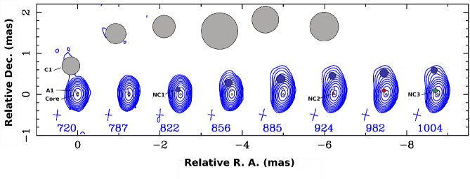
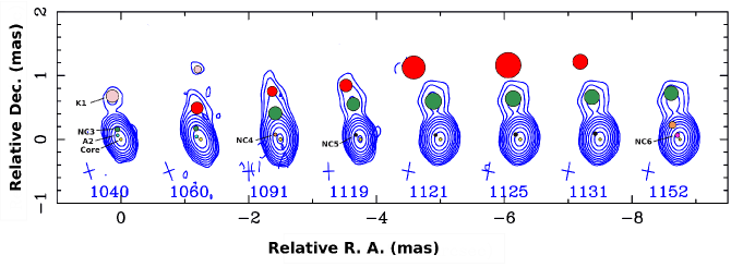
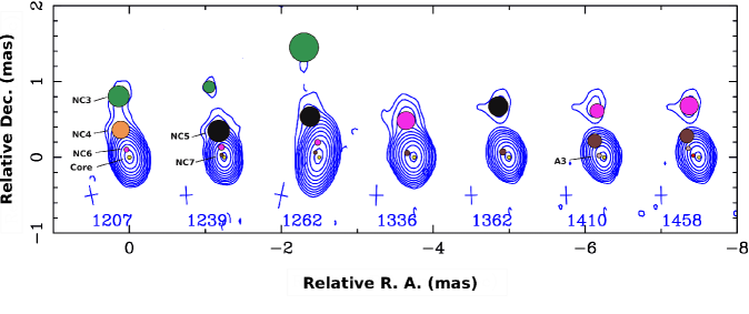
Figure 1: 43 GHz VLBA images (contours) and Gaussian components of S5 0716+714 at different epochs between September 2008 and October 2010. The date of observation is given at the bottom of each map (shifted Julian day, JD$-$2454000). The fitted model parameters for each epoch are given in Table A. The cross at the bottom of each map represents the FWHM of the restoring beam (0.25$\times$0.18 mas). Contour levels correspond to -0.003 0.003 0.006 0.012 0.024 0.048 0.096 0.19 0.38 0.76 1.54 3.07 6.14 12.28 24.58 49.15 98.30 mJy/beam.

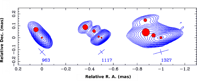
Figure 2: The inner jet structure of S5 0716+714 from GMVA observations at 3 mm. The cross at the bottom of each map represents the FWHM of the restoring beam (0.07$\times$0.04 mas). Contour levels correspond to -0.004 0.004 0.008 0.016 0.032 0.064 0.12 0.25 0.51 1.02 2.04 4.09 8.19 16.38 32.77 65.54 mJy/beam.

3.1 Jet kinematics

Figures 1 and 2 display a sequence of VLBI maps convolved with a natural beam. The model fit parameters are given in Table A. In the following sub-sections, we will discuss in detail the apparent motions of components and brightness temperature gradient in the parsec-scale jet.

3.1.1 Component motion

For the kinematic study of individual components, we choose the VLBI core as a reference point, fixed to coordinates (0,0). However, it is important to note that the absolute position of the reference point i.e. core may change e.g. due to changes in opacity or instabilities in the jet; but, the results presented here are not sensitive to that as we are interested in the relative motion of components w.r.t. the core. The VLBI data were fitted by using different numbers of components during different activity stages over the time span considered here. During this period, we identified a total of 12 components - C1, K1, A1, A2, A3, and NC1 to NC7 - in addition to the core, C0 (see Fig. 1). Figure 3 plots the evolution of the distance of different knots from the core, and Fig. 4 shows their trajectories in the XY-plane projected on the sky.

Stationary Features :
The sequence of VLBI images allow us to investigate the component motion along the jet as a function of time. Most of the components exhibit significant motion down the jet, except A1, A2, and A3. The latter are comparatively stable in position, although they exhibit significant scatter in position angle exceeding the uncertainties (see Fig. 4). Nevertheless, their radial distance from the core remains at $\sim$0.15 mas. Stationary features are a common characteristic in AGN jets (e.g., Fromm et al., 2013a; Jorstad et al., 2001; Britzen et al., 2010). In straight jets, these can be produced by recollimation shocks, instabilities [magnetohydrodynamic (MHD), and/or Kelvin-Helmholtz (KH)], or magnetic pinches (see Marscher, 2009; Hardee, 2006; Meier et al., 2001, for details). Bends in the jet can also cause quasi-stationary features, either because the jet turns more into the line of sight, thus increasing the Doppler beaming factor, or due to the formation of a shock that deflects the flow (Alberdi et al., 1993). Numerical simulations indicate that when a moving knot passes through a standing re-collimation shock, the components blend into a single feature, then split up after the collision with no lasting changes in the proper motion of the moving knot (Gomez et al., 1997; Fromm et al., 2012). During the interaction, the feature may move a short distance downstream before returning to its previous position. Therefore, it is quite possible that A1, A2, and A3 are the same standing feature, which becomes disturbed by moving features. We find that the kinematics of three new components NC2, NC3, and NC6, are significantly different before and after the interaction. The components move more slowly ($\beta_{app}\leq 10c$) as they approach the stationary feature, then faster ($\beta_{app}\geq 20c$) after the interaction. Such behavior is consistent with the stationary feature representing a bend in the jet (Alberdi et al., 1993). Indeed, a bend at $\sim$0.15 mas is evident in the 3 mm maps of the source (see Fig. 2). This suggests that the observed stationary features are standing oblique shocks that cause the flow of the jet to bend at $\sim$0.15 mas owing to a transverse pressure gradient or an impact with an interstellar cloud.

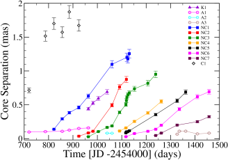
Figure 3: Evolution of core separation of the individual components as a function of time.

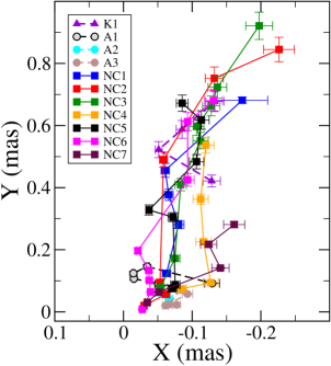
Figure 4: Trajectories of the jet knots in the X-Y plane, where X = r.cos($\mathrm{\theta}$ + 90) and Y = r.sin($\mathrm{\theta}$ + 90) (r is the radial separation from the core and ${\rm\theta}$ is the position angle with respect to an imaginary north-south line drawn through the map center).

Moving Features :
The other components, C1, K1, and NC1 to NC7, exhibited significant motion in the radial direction. Component C1 represents very faint emission at a core separation of $\geq$1 mas. It seems to be the remnants of a component ejected in earlier epochs. The bright feature K1 could be a trailing component that forms behind a strong shock (Agudo et al., 2001) as it is identified at four epochs after the ejection of a new component (NC1).

As seen in Fig. 4, all components follow curved trajectories in the XY-plane projected on the sky. In addition, the trajectories differ from one component to the next. The wiggling trajectories in the jet might be a signature of helical motion. Helical jet models (e.g., Gomez et al., 1994; Hardee, 2006) represent the jet as an inhomogeneous flow of plasma interacting with ambient matter. Magnetohydrodynamic or Kelvin-Helmholtz instabilities (Hardee, 2006; Perucho et al., 2006) can explain the bending and helical structures, and possibly also less regular wiggles observed in parsec-scale radio jets.

In order to investigate component motions in the jet of S5 0716+714, we use the XY positions of the components relative to the core to fit the trajectories with polynomials of different order. The resulting fitted radial separation of each component, $r(t)=\sqrt{x(t)^{2}+y(t)^{2}}$, is shown in Fig. 5. We find that a linear function is sufficient to fit the trajectories of components NC1, NC4, NC5, and NC7. However, a second-order polynomial is required to fit the trajectories of components NC2, NC3, and NC6, which corresponds to an apparent acceleration. Two multiple straight lines needed to fit different portions of the trajectories of these components in Fig. 5 provides a clear demonstration of the inadequacy of simple linear fits. The dashed curves represent the quadratic fits.

For each component, the fits yield an average proper motion and a mean speed. Using the estimated angular speed $\mu$, we have computed the kinematic parameters of the jet, e.g., the apparent speed, $\beta_{app}$, and Doppler factor, $\delta$. We derive the apparent speed of the components, $\beta_{app}$, from the angular speed, $\mu$, using

$$\beta_{app}=\frac{\mu\leavevmode\nobreak\ d_{L}}{c(1+z)},$$ (1)

where $d_{L}$ is the luminosity distance and $z$ the redshift of the source. The luminosity distance $d_{L}$ corresponding to z=0.3 is $d_{L}$ = 1600 Mpc for a $\Lambda$CDM cosmology with $\Omega_{m}$ = 0.27, $\Omega_{\lambda}$ = 0.73, and $H_{0}$ = 71 km s^-1 Mpc^-1 (Spergel et al., 2003). The angular and apparent speed of the individual components are given in Table 1. The calculated $\beta_{app}$ values range from $6c$ to $37c$, the latter of which is unusually high for a blazar, especially for a BL Lac object.

For the non-ballistic components, NC2, NC3, and NC6, the quadratic fits represent significant acceleration along the jet axis. Formally, we obtain $\dot{\mu}$ = 4.90$\pm$1.55 mas yr^-2 for NC2, $\dot{\mu}$ = 2.45$\pm$0.80 mas yr^-2 for NC3, and $\dot{\mu}$ = 0.94$\pm$0.36 mas yr^-2 for NC6. Such apparent acceleration is a commonly observed feature of many objects in the MOJAVE sample (Lister et al., 2013), for which a statistically significant tendency for acceleration in the base of jets has been found. A standing shock slows the flow while deflecting it, after which the flow can accelerate back to the velocity it had upstream of the shock (Gomez et al., 1997). However, since the apparent speed was relatively slow in the upstream region, this seems not to fit the case of S5 0716+714. The data are more consistent with the scenario that, after a moving component passes through the stationary feature, it bends towards or away from our line-of-sight. It then appears to move faster because its velocity vector subtends an angle closer to that which maximizes apparent motion, $\arccos(\beta)$, where $\beta$ is the velocity of the component divided by the speed of light. An alternative possibility is that the underlying flow of the jet systematically accelerates outward. Theoretical models involve strong magnetic fields associated with the putative supermassive black hole/accretion disk system that play a key role in the initial acceleration and collimation of the jet (Blandford & Payne, 1982; Blandford & Znajek, 1977; Meier et al., 2001). The conversion of Poynting flux to flow energy is gradual and may persist out to parsec scales (e.g., Sikora et al., 2005). Under this explanation, however, it is difficult to explain the straight-line kinematic evolution of some of the components.

Variability Doppler factor:
A variability Doppler factor using VLBI jet kinematics was defined by Jorstad et al. (2005) as

$$\delta_{VLBI}=\frac{sd_{L}}{c\Delta t_{var}(1+z)},$$ (2)

where $s$ is the angular size of the component, defined as 1.6$\times$$\phi$ for a Gaussian with FWHM diameter $\phi$ measured at the epoch of maximum brightness, and $d_{L}$ is the luminosity distance. The timescale of variability is defined as $\Delta t_{var}$ = $dt/ln(S_{max}/S_{min})$ (Burbidge et al., 1974), where $dt$ is the time separation in years between maximum ($S_{max}$) and minimum ($S_{min}$) flux densities. The estimated values of $\delta_{VLBI}$ for the individual components, listed in Table 1, range from 6 to 21. Using the broadband flux density and spectral variability study of the source over the same time period (Paper I, Sect. 3.4), we obtain a range of self-consistent values for the Doppler factor. The different independent approaches suggest that $\delta\geq$20, which is consistent with upper range of the values of $\delta_{VLBI}$ obtained here.

3.1.2 Ejection Epochs

Back-extrapolation of the components’ motion allows us to estimate the time of zero separation from the core (i.e., the “ejection” time, T₀). As shown in the previous section, the components follow curved trajectories; therefore, we back-extrapolate the component trajectories in the XY-plane to determine the epoch of (0,0) separation. The error estimates are not very straightforward to calculate for components following non-ballistic trajectories. We use the estimated error on the fitted parameters for a given function to calculate its uncertainty. Back-extrapolation of the two envelopes of the function provide us with the error in T₀. The calculated ejection times for the individual components are listed in Table 1.

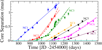
Figure 5: Evolution of radial separation of different components from the core. The solid lines represent fits with linear functions, while the dashed curves are quadratic fits.

Table 1: Physical parameters of the radio emission

Component	$\mu$ (mas/yr)	$\beta_{app}(c)$	$\delta_{var}$	T0 (days)
NC1	1.30$\pm$0.04	24.88$\pm$0.88	7.03$\pm$0.35	783${}^{+16}_{-12}$
NC2l	0.45$\pm$0.00	8.71$\pm$0.13	13.84$\pm$0.69	900${}^{+10}_{-16}$
NC2u	1.93$\pm$0.14	37.06$\pm$2.75
NC3l	0.61$\pm$0.03	11.69$\pm$0.64	6.02$\pm$0.30	933${}^{+19}_{-12}$
NC3u	1.87$\pm$0.17	35.78$\pm$3.29
NC4	0.87$\pm$0.04	16.81$\pm$0.95	6.91$\pm$0.34	1047${}^{+12}_{-9}$
NC5	0.85$\pm$0.03	16.30$\pm$0.59	11.72$\pm$0.58	1079${}^{+5}_{-6}$
NC6l	0.34$\pm$0.04	6.53$\pm$0.77	15.33$\pm$0.76	1092${}^{+26}_{-17}$
NC6u	0.99$\pm$0.04	19.05$\pm$0.92
NC7	0.48$\pm$0.04	9.20$\pm$0.84	20.96$\pm$1.04	1203${}^{+11}_{-16}$

$l$ and $u$ denote, respectively, lower and upper values of the component speeds.

3.1.3 Brightness temperature gradient in the jet

The redshift-corrected brightness temperature (T_B,obs) of the bright emission features can be approximated using the following relation (Jorstad et al., 2005):

$$T_{B,obs}=1.22\times 10^{12}\frac{S_{comp}}{(1+z)\leavevmode\nobreak\ d_{comp}^{2}\leavevmode\nobreak\ \nu^{2}}\,\leavevmode\nobreak\ {\rm K},$$ (3)

where $S_{comp}$ is the component flux density in Jy, $d_{comp}$ is the FWHM of the circular Gaussian component in mas, and $\nu$ is the observing frequency in GHz; for the calculations here, we have only used 43 GHz data. The calculated brightness temperatures ($T_{B,obs}$) of the components generally decline with radial separation from the core (see Fig. 8). This decaying trend can be approximated by a power law, $T_{B,obs}\sim r_{jet}^{-\epsilon}$ with $\epsilon$ = 2.43$\pm$0.36, where $r_{jet}$ is the radial distance along the jet axis. The solid line in Fig. 8 represents the fitted power law.

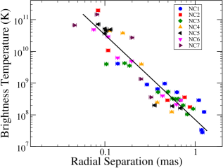
Figure 6: Component brightness temperature as a function of radial separation from the core. The solid line represents the fitted power law with index $\epsilon=2.43\pm 0.36$.

We place the observed brightness temperature gradient in the context of the shock-in-jet model (Marscher & Gear, 1985). In the common picture of this model, a relativistic shock propagates down a conical jet, slowly expanding adiabatically while maintaining shock conditions during propagation. While the shock propagates down the jet, it undergoes three major evolutionary stages dominated by inverse Compton, synchrotron, and adiabatic energy losses. As a result, the observed brightness temperature declines as a power law, T_B,obs $\propto r_{jet}^{-\epsilon}$. The value of $\epsilon$ can be derived from the spectral evolution of the radio emission (Lobanov & Zensus, 1999; Fromm et al., 2013b). Following $T_{B}\propto$ $S_{\nu}r_{jet}^{-2}\nu^{-2}$ and S($\nu$) $\propto r_{jet}^{\xi}\nu^{\zeta}\delta^{(s+3)/2}$ (Lobanov & Zensus, 1999), we obtain

$$\epsilon_{Compton}=\frac{11-s-a(s+1)}{8}+\frac{b(s+3)}{2}-2,$$ (4)

$$\epsilon_{synchrotron}=\frac{-[4(s-1)+3a(s+1)]}{6}+\frac{b(s+3)}{2}-2,$$ (5)

and

$$\epsilon_{adiabatic}=\frac{2(5-2s)-3a(s+1)}{6}+\frac{b(s+3)}{2}-2,$$ (6)

where $a$, $b$, and $s$ parametrize the variations along the jet axis of the Doppler factor, $\delta\propto r_{jet}^{b}$, magnetic field, $B\propto r_{jet}^{-a}$, and power law distribution of energy of the emitting electrons, $N(\gamma)\propto\gamma^{-s}$. Assuming a constant Doppler factor, i.e., $b$ = 0, and using a typical value of $s$ = 2 (corresponding to optically thin synchrotron spectral index = $-$0.5), and $a$ = 1 to 2 (for toroidal and poloidal magnetic fields, respectively), we obtain $\epsilon_{Compton}$ = 1.3 to 1.6, $\epsilon_{synchrotron}$ = 4.2 to 5.7, and $\epsilon_{adiabatic}$ = 3.2 to 4.7.

The observed brightness temperature gradient in S5 0716+714 (Fig. 8) has a slope equal to 2.43$\pm$0.36. The slope of the observed intensity gradient rules out the simple assumptions of a constant Doppler factor. We therefore consider a variable Doppler factor along the jet axis. We find that the observed value of $\epsilon$ is consistent with the adiabatic loss phase if $\delta\propto$ $r_{jet}^{b}$, with $b$ $\sim$ 0.12 to 0.40, which corresponds to a moderate variation in the Doppler factor. However, with relatively larger variations in the Doppler factor $b$ $\sim$ 0.47 to 0.74, the observed value of $\epsilon$ would agree with synchrotron loss phase as well.

The evolution of the flux density and frequency ($S_{m}$ and $\nu_{m}$) at the spectral turnover from synchrotron self-absorption of the radio flares, discussed in Paper I (Section 3.3.2), also suggests a variation of $\delta$ along the jet axis. In that study, we found that $\delta$ changes as $r_{jet}^{b}$ with $b=0.7$ during the rise and $b=2.6$ during the decay of the first radio flare. The evolution of the second flare was governed by $b=0.4$ during the rising phase and $b=-2.0$ during the decay (see Paper I for details). Therefore, it is evident that the two flares require a different dependence of $\delta$ on distance from the core, which is also inconsistent with what we obtained for the brightness temperature gradient ($b=0.12$ to 0.74). This can be explained in two ways. First, the single-dish radio flux correlates well with the VLBI core flux (see Section 3.2 for details). This implies that the radio flares originate within the core. The core is more compact and farther upstream than the jet components, with a comparatively higher brightness temperature, and can follow a different dependence of $\delta$ on $r_{jet}$. The individual components trace the intensity gradient further downstream of the jet, and therefore can individually have a different $\delta$ – $r_{jet}$ dependence. A second possibility is that the brightness temperature gradient plot corresponds to an averaged behavior of the two radio flares.

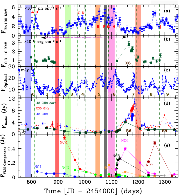
Figure 7: Broadband flux light curves of S5 0716+714: (a) weekly averaged $\gamma$-ray flux light curve at E$>$100 MeV, (b) X-ray light curve at 0.3–10 keV, (c) optical V-band light curve, (d) single-dish (43 and 230 GHz) and 7 mm VLBI core flux light curves, and (e) flux density curves of moving jet components shown in different colors; the same color is used to shade their respective ejection times, i.e., epochs of zero separation from the core. The green dashed lines indicate the average times when moving components cross the stationary feature at $\sim$0.15 mas. The major outburst is marked with a horizontal arrow; the faster repetitive optical flares are labeled as “0” to “9” and sharp $\gamma$-rays flares as “A” to “J” (see text for details).

3.2 Jet kinematics and broadband emission

For the comparison of the observed broadband flaring behavior with the jet kinematics, we have used the flux density light curves from Paper I, where the details of observations and data reduction are given. Broadband flux light curves are shown in Fig. 7. Panel (a) presents the weekly averaged $\gamma$-ray photon flux light curve. Panel (b) shows the X-ray light curve, while panel (c) displays the optical V-band light curve. Panel (d) presents the radio (single-dish) and 43 GHz core flux density curves plotted in the same panel. Panel (e) exhibit flux density light curves of the individual components shown in different colors, with the same color used to shade their respective ejection times. The major outburst between JD’ $\sim$840 and 1150 is marked with a horizontal arrow in panel (b). The repetitive optical flares with a typical duration of $\sim$120–140 days are label as “0” to “9”, and the broadband flares are denoted “G” for $\gamma$-rays, “X” for X-rays, “O” for optical and “R” for radio followed by the number adjacent to them; e.g., we have flares G0 to G9 at $\gamma$-rays, X6 at X-rays, O0 to O9 at optical, and R6 and R9 at radio frequencies. The sharp $\gamma$-ray flares are labeled as “A” to “J”, and have a duration of $\sim$10–20 days.

Although VLBI observations of S5 0716+714 are missing at the peak of the two major radio flares (JD’ $\sim$ 1150–1200 and $\sim$1300), there is still an apparent one-to-one correlation between the core flux and single-dish radio flux measurements. This suggests that the single-dish radio flares are produced in the core, which agrees with the high mean core-to-jet flux ratio, which ranges from 1.3 to 21.4 with a mean of 4.9$\pm$4.0. The broadband flux cross-correlations (Paper I) also indicate that the flux variations at $\gamma$-ray (and optical) and single-dish radio frequencies are correlated such that the peak of the major optical/$\gamma$-ray outburst leads the peak of the radio outburst by a two-month time period.

3.2.1 Component ejections and their connection with broadband flares

Because of the superposition of different modes of flaring activity, the broadband flaring behavior is quite complex in the source. The major outburst (marked with a horizontal arrow in Fig. 7) is accompanied by faster repetitive optical/$\gamma$-ray flares (labeled as “0” to “9”) and sharp $\gamma$-rays flares (labeled as “A” to “J”). The jet kinematic study during this period suggests significant changes in the jet morphology of the source; in total, seven new components were ejected. It is therefore plausible that the ejection of new components could be connected to the broadband flares. We have identified a stationary feature at a distance of $\sim$0.15 mas from the core (Section 3.1.1). Interaction of a moving component with the stationary feature could amplify the magnetic field and accelerate particles to produce a multi-waveband flare (Marscher, 2014; Fromm et al., 2012).

Table 2: Component ejection epochs and broadband flares

Component	Flares observed at the time of
	zero separation	component crosses
	from the core	stationary feature
NC1	O0/G0	G0B
NC2	O2/G2	G4C
NC3	O3/G3	O4D
NC4	O5E/G5E	O6G/G6G
NC5	O5F/G5F	G6I
NC6	O6/G6	–
NC7	R6	O9J/G9J

In Fig. 7, the shaded areas represent the ejection times of new jet components and the green dashed lines mark the average epochs when a moving component crosses the stationary feature at $\sim$0.15 mas. In Table LABEL:tab3, we list the new components (col. 1), along with the flares that coincide with their respective ejection times (col. 2). Flares observed closer in time to the passage of a moving component across the stationary feature are listed in col. 3. We note that most of the sharp $\gamma$-ray flares (B, C, D, G, I, and J) are observed when a moving component crosses the stationary feature, while most of the repetitive faster flares (0, 2, 3, 5, and 6) coincide with the ejections of new components from the core.

In Paper I, we found that the high-energy (optical and $\gamma$-ray) emission is significantly correlated with the radio flares such that the major optical/$\gamma$-ray outburst propagates down to radio frequencies (R6 flare) with a time delay of $\sim$65 days, following a power-law dependence on frequency with a slope $\sim$0.3. We also noticed that the evolution of radio flare R6 is in accordance with a generalized shock model (Valtaoja et al., 1992). This suggests that the origin of the major outburst could be related to a disturbance/shock that moves down the jet.

We interpret the broadband flaring events in the following manner (see Fig. 8). A disturbance at the base of the jet could cause a shock wave to form and propagate down the jet (Valtaoja et al., 1992; Marscher & Gear, 1985), which could be related to the onset of the major optical/$\gamma$-ray outburst (JD’ $\sim$840) and disturbs the jet outflow, resulting in the ejection of two new components (NC2 and NC3, Fig. 8a). The core is optically thick at that point, as the shock forms upstream of the core; for this reason, we do not see much activity in the core. Repetitive optical/$\gamma$-ray flares and the curved trajectories of the associated components favor the propagation of the shock along a bent trajectory, possibly a helical path. The moving shock reaches its maximum strength at JD’ $\sim$1150 (Fig. 8 b), close to the peak of the major optical/$\gamma$-ray outburst (see Section 3.3, Paper I for details), which also coincides with the onset of radio flare R6. At this point, the shock reaches the core, which starts to become optically thin. After this, further disturbances passing through the core correspond to the ejections of three new components (NC3, NC4, and NC5). Major radio outburst R6 is observed $\sim$65 days later, accompanied by the ejection of component NC7 (Fig. 8 c). As the moving features cross the the stationary feature at $\sim$0.15 mas, at first, the stationary feature gets destructed after the interaction, and later it appears again. The times of passage of moving components through the stationary feature appear to coincide with the sharp $\gamma$-ray flares in most cases. Therefore, the sharp $\gamma$-ray flares seem to be produced via the interaction of moving features with the stationary one.

X-ray flare X6 coincides with a similar increase in the flux of the 43 GHz core. Optical flare O7 peaks about a month later, which roughly coincides with the expected passage through the stationary feature of the same disturbance that caused flare X6. However, no bright moving knot is apparent in the next VLBA image $\sim 20$ days after O7. Also, the dramatic decrease in the millimeter-wavelength flux during this interval implies that the disturbance is strongly quenched following flare O7. There are two anomalies in this sequence of events: there is no optical flare as the disturbance crosses the core, and there is no $\gamma$-ray activity during the entire time span covering flares X6 and O7. The first indicates that, for reasons that are unclear (e.g., non-favorable magnetic field orientation relative to a shock; Summerlin & Baring, 2012), electrons with energies high enough to produce optical and $\gamma$-ray emission were not produced in the core region at this time. The second implies that there was a dearth of seed photons for inverse-Compton scattering $\sim$0.15 mas from the core during flare O7.

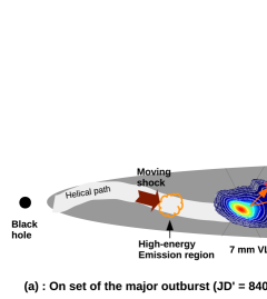
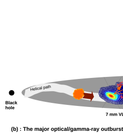
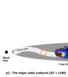
Figure 8: Sketch for the proposed scenario in the BL Lac S5 0716+714 (not to scale). Note that north is to the right in this sketch. A shock propagates down the jet along a helical path, producing a major optical/$\gamma$-ray outburst upstream of the 7 mm VLBI core and later a major radio outburst accompanied by ejection of components from the core.

3.2.2 Doppler beaming of radio and gamma-ray emission regions

The observed time lag between $\gamma$-ray and 43 GHz core flares can be used to estimate the separation between the two emission regions by using the following equation (Fuhrmann et al., 2014):

$$\Delta r_{\mathrm{\gamma,r}}=\frac{\beta_{\mathrm{app}}c\,\tau_{\mathrm{\gamma,r}}}{\sin\theta},$$ (7)

where $\theta$ is the viewing angle of the source, $\beta_{\mathrm{app}}$ is the apparent jet speed, and $\tau_{\mathrm{\gamma,r}}$ is the observed time lag. Using the observed value $\tau_{\mathrm{\gamma,r}}$ = 82$\pm$32 days (Rani et al., 2014), we have $\Delta r_{\mathrm{\gamma,r}}$ = (0.069$\pm$0.026)$\beta_{\mathrm{app}}$($\sin\theta$)^-1 pc.

The measured apparent speeds in the source cover a wide range. The current observations suggest slower motion ($\leq$8 c) on sub-mas scales ($\sim$0.3 mas), which later get accelerated to speeds as fast as 40 c on mas scales. The source also has a prominent bent jet structure at sub-mas scales (see Fig. 2); as a result, the sub-mas and mas regions could have different viewing angles. For $\beta_{\mathrm{app}}$ = 6-8 c, the viewing angle, $\theta$, is 6-9^∘; this gives $\Delta r_{\mathrm{\gamma,r}}$ = 2.9-4.4 pc. Using $\beta_{\mathrm{app}}$ = 40 c, we have $\theta$ = 1.4^∘ and $\Delta r_{\mathrm{\gamma,r}}$ $\sim$ 110 pc. Even for a larger viewing angle, $\theta$=10^∘, we obtain $\Delta r_{\mathrm{\gamma,r}}$ $\sim$16 pc. Pushkarev et al. (2012) estimated that the 15 GHz core is located at a distance of 6.68 pc from the jet base/apex. Using the technique to align the optically-thin emission based on model-fitted components and morphological similarities, we derive a shift of 0.042$\pm$0.013 mas (0.19$\pm$0.06 parsec) between the 15 GHz and 43 GHz core, which puts the location of the 43 GHz core at a distance of $\sim$6.5 pc from the jet-apex. Therefore, the distance between $\gamma$-ray emission region and 43 GHz core cannot be larger than 6.5 pc. For a typical viewing angle $\theta\leavevmode\nobreak\ \approx 5^{\circ}$, $\Delta r_{\mathrm{\gamma,r}}$ $\leq$ 6.5 pc gives $\beta_{\mathrm{app}}$ $\leq$ 8 c. However, we note that for a larger viewing angle ($\theta$ $\sim$ 10^∘), $\beta_{\mathrm{app}}$ could be as high as 10-12$c$ but not $\sim 40c$ unless the viewing angle is larger than 30^∘, which is unlikely to be the case for S5 0716+714. The results therefore suggest that the high-energy and radio emission regions have different apparent speeds and probably different viewing angles as well. This implies that the $\gamma$-ray and radio emission regions have different Doppler factors.

4 Summary and conclusion

The monthly sampled mm-VLBI monitoring of S5 0716+714 allows us to study the inner jet kinematics and to investigate its relation to the observed broadband flux variability. Our study reveals significant non-radial motions in the jet outflow, including variations in the orientation of the sub-parsec-scale jet (see Rani et al. 2014 for details) and possibly helical trajectories of moving components.

In radial directions, the individual components exhibit extreme apparent speeds as high as $\sim$37 c. An apparent speed of $\sim$20 c seems to be more typical in S5 0716+714 on parsec scales. Recently, Lister et al. (2013) reported an apparent speed of 43.6$\pm$1.3 c. These values would even be extreme for a quasar. Therefore, moving components in the jets of BL Lac objects can be just as fast as in quasars, despite flux-limited surveys at lower resolution (e.g. Lister et al., 2009) finding that the mean apparent velocity of BL Lac objects is lower than for quasars. Further mm-VLBI studies are needed to determine the extent to which angular resolution and the variety of spectral classes of BL Lac objects (low- to high-frequency peaks of the synchrotron spectral energy distributions) skew the apparent velocity distribution. It is possible that the fast BL Lacs are actually quasars in disguise, with their broad emission lines swamped by the non-thermal optical continuum. On the other hand, emission lines have never been observed in S5 0716+714.

The bright components in 0716+714 follow a continuous decay trend in the observed brightness temperature (T${}_{B,obs}\propto r_{jet}^{-(2.36\pm 0.41)}$), which implies a variation in Doppler factor along the jet axis. The spectral evolution of radio flares (see Paper I for details) also suggests variations in Doppler factor. A significant correlation between $\gamma$-ray flux and variations in orientation of the sub-parsec scale jet (Rani et al., 2014) supports the possibility that the observed flux variations in S5 0716+714 are strongly influenced by Doppler factor variations, and therefore may have a geometrical origin.

Our study suggests a connection between jet kinematics and the observed broadband flaring activity. We find that the origin of major optical/$\gamma$-ray/radio outbursts in the source seems to be related to a disturbance, such as shock wave, propagating down the jet. The repetitive, faster optical/$\gamma$-ray flares, superposed on the major outbursts, and non-ballistic motions of the associated jet components can be interpreted via helical jet models (as discussed by, e.g., Blandford & Payne, 1982; Blandford & Znajek, 1977; Camenzind & Krockenberger, 1992) and/or magnetohydrodynamic instabilities (Hardee, 2006). Our analysis favors that the major optical/$\gamma$-ray flares in S5 0716+714 are produced upstream of the 7 mm VLBI core. The sharp $\gamma$-ray flares, however, seem to be produced when the moving components cross a stationary feature 0.15 mas from the core. Finally, our analysis suggests that the upstream $\gamma$-ray emission region has a different Doppler factor than observed in the parsec-scale radio jet.

Appendix A Model fit component results

Table 3: Results from Gaussian Model fitting and component parameters

Epoch (JD′)	Speak	r	$\theta$	$\phi$	Compa	Wavelength
Date	(Jy/beam)	(mas)	(∘)	(mas)
720	1.670$\pm$0.084	0$\pm$0	0$\pm$0	0.044$\pm$0.002	core	7 mm
10.09.2008	0.139$\pm$0.007	0.098$\pm$0.005	39.90$\pm$2.00	0.034$\pm$0.002	A1
	0.023$\pm$0.001	0.714$\pm$0.036	13.28$\pm$0.66	0.427$\pm$0.021	C1
787	1.670$\pm$0.084	0$\pm$0	0$\pm$0	0.038$\pm$0.002	core	7 mm
16.11.2008	0.188$\pm$0.009	0.103$\pm$0.005	29.29$\pm$1.46	0.071$\pm$0.004	A1
	0.022$\pm$0.001	1.516$\pm$0.076	12.33$\pm$0.62	0.487$\pm$0.024	C1
822	2.044$\pm$0.102	0$\pm$0	0$\pm$0	0.034$\pm$0.002	core 7 mm
21.12.2008	0.082$\pm$0.004	0.139$\pm$0.007	26.83$\pm$1.34	0.101$\pm$0.005	NC1
	0.013$\pm$0.001	1.700$\pm$0.085	13.57$\pm$0.68	0.538$\pm$0.027	C1
856	2.167$\pm$0.108	0$\pm$0	0$\pm$0	0.034$\pm$0.002	core 7 mm
24.01.2009	0.405$\pm$0.020	0.108$\pm$0.005	8.06$\pm$0.40	0.045$\pm$0.002	A1
	0.052$\pm$0.003	0.292$\pm$0.015	15.92$\pm$0.80	0.171$\pm$0.009	NC1
	0.025$\pm$0.001	1.572$\pm$0.079	11.01$\pm$0.55	0.879$\pm$0.044	C1
885	1.717$\pm$0.086	0$\pm$0	0$\pm$0	0.035$\pm$0.002	core	7 mm
22.02.2009	0.420$\pm$0.021	0.125$\pm$0.006	6.64$\pm$0.33	0.051$\pm$0.003	A1
	0.053$\pm$0.003	0.383$\pm$0.019	9.89$\pm$0.49	0.201$\pm$0.010	NC1
	0.016$\pm$0.001	1.873$\pm$0.094	13.47$\pm$0.67	0.642$\pm$0.032	C1
924	1.038$\pm$0.052	0$\pm$0	0$\pm$0	0.018$\pm$0.001	core	7 mm
02.04.2009	0.552$\pm$0.028	0.036$\pm$0.002	56.28$\pm$2.81	0.036$\pm$0.002	NC2
	0.187$\pm$0.009	0.150$\pm$0.008	13.26$\pm$0.66	0.062$\pm$0.003	A1
	0.051$\pm$0.003	0.460$\pm$0.023	7.60$\pm$0.38	0.163$\pm$0.008	NC1
	0.020$\pm$0.001	1.672$\pm$0.084	8.84$\pm$0.44	0.692$\pm$0.035	C1
963	0.354$\pm$0.018	0$\pm$0	0$\pm$0	0.011$\pm$0.001	core	3 mm
11.05.2009	0.104$\pm$0.005	0.028$\pm$0.001	73.33$\pm$3.67	0.012$\pm$0.001	NC3
	0.043$\pm$0.002	0.084$\pm$0.004	47.52$\pm$2.38	0.025$\pm$0.001	NC2
	0.048$\pm$0.002	0.159$\pm$0.008	54.57$\pm$2.73	0.030$\pm$0.001	A1
	0.030$\pm$0.001	0.441$\pm$0.022	16.93$\pm$0.85	0.047$\pm$0.002	K1
	0.019$\pm$0.001	0.628$\pm$0.031	39.92$\pm$2.00	0.044$\pm$0.002	NC1
982	0.482$\pm$0.024	0$\pm$0	0$\pm$0	0.038$\pm$0.002	core	7 mm
30.05.2009	0.118$\pm$0.006	0.109$\pm$0.005	29.31$\pm$1.47	0.074$\pm$0.004	NC2
	0.035$\pm$0.002	0.525$\pm$0.026	5.61$\pm$0.28	0.192$\pm$0.010	K1
1004	0.548$\pm$0.027	0$\pm$0	0$\pm$0	0.039$\pm$0.002	core	7 mm
21.06.2009	0.075$\pm$0.004	0.104$\pm$0.005	31.10$\pm$1.56	0.097$\pm$0.005	NC3
	0.022$\pm$0.001	0.594$\pm$0.030	8.26$\pm$0.41	0.148$\pm$0.007	K1
	0.564$\pm$0.028	0$\pm$0	0$\pm$0	0.035$\pm$0.002	core	7 mm
1040	0.166$\pm$0.008	0.080$\pm$0.004	39.50$\pm$1.98	0.040$\pm$0.002	A2
27.07.2009	0.038$\pm$0.002	0.165$\pm$0.008	19.10$\pm$0.96	0.067$\pm$0.003	NC3
	0.010$\pm$0.001	0.690$\pm$0.035	11.10$\pm$0.56	0.187$\pm$0.009	K1
1060	0.663$\pm$0.033	0$\pm$0	0$\pm$0	0.039$\pm$0.002	core	7 mm
16.08.2009	0.125$\pm$0.006	0.079$\pm$0.004	56.40$\pm$2.82	0.040$\pm$0.002	A2
	0.030$\pm$0.002	0.188$\pm$0.009	23.50$\pm$1.18	0.066$\pm$0.003	NC3
	0.019$\pm$0.001	0.494$\pm$0.025	6.77$\pm$0.34	0.181$\pm$0.009	NC2
	0.006$\pm$0.000	1.098$\pm$0.055	2.52$\pm$0.13	0.104$\pm$0.005	NC1
1091	0.873$\pm$0.044	0$\pm$0	0$\pm$0	0.045$\pm$0.002	core	7 mm
16.09.2009	0.172$\pm$0.009	0.112$\pm$0.006	48.70$\pm$2.44	0.044$\pm$0.002	NC4
	0.041$\pm$0.002	0.388$\pm$0.019	11.50$\pm$0.58	0.199$\pm$0.010	NC3
	0.015$\pm$0.001	0.764$\pm$0.038	9.97$\pm$0.50	0.147$\pm$0.007	NC2
1117	0.356$\pm$0.018	0$\pm$0	0$\pm$0	0.012$\pm$0.001	core	3 mm
12.10.2009	0.110$\pm$0.005	0.029$\pm$0.001	73.71$\pm$3.69	0.015$\pm$0.001	NC6
	0.041$\pm$0.002	0.084$\pm$0.004	48.90$\pm$2.45	0.017$\pm$0.001	NC5
	0.042$\pm$0.002	0.158$\pm$0.008	53.49$\pm$2.67	0.024$\pm$0.001	NC4
	0.021$\pm$0.001	0.502$\pm$0.025	17.16$\pm$0.86	0.040$\pm$0.002	NC3
1119	0.835$\pm$0.042	0$\pm$0	0$\pm$0	0.039$\pm$0.002	core	7 mm
14.10.2009	0.122$\pm$0.006	0.100$\pm$0.005	47.00$\pm$2.35	0.041$\pm$0.002	NC5
	0.025$\pm$0.001	0.563$\pm$0.028	11.50$\pm$0.58	0.197$\pm$0.010	NC3
	0.013$\pm$0.001	0.875$\pm$0.044	15.00$\pm$0.75	0.189$\pm$0.009	NC2
1121	1.142$\pm$0.057	0$\pm$0	0$\pm$0	0.040$\pm$0.002	core	7 mm
16.10.2009	0.175$\pm$0.009	0.100$\pm$0.005	48.10$\pm$2.41	0.041$\pm$0.002	NC5
	0.038$\pm$0.002	0.607$\pm$0.030	10.30$\pm$0.52	0.248$\pm$0.012	NC3
	0.007$\pm$0.000	1.201$\pm$0.060	20.30$\pm$1.02	0.352$\pm$0.018	NC1
1125	1.204$\pm$0.060	0$\pm$0	0$\pm$0	0.039$\pm$0.002	core	7 mm
20.10.2009	0.243$\pm$0.012	0.103$\pm$0.005	43.20$\pm$2.16	0.052$\pm$0.003	NC5
	0.036$\pm$0.002	0.648$\pm$0.032	9.79$\pm$0.49	0.238$\pm$0.012	NC3
	0.010$\pm$0.001	1.177$\pm$0.059	9.19$\pm$0.46	0.391$\pm$0.020	NC1

JD^′ = JD - 2454000,
S_peak : The integrated flux in the component,
r : The radial distance of the component center from the center of the map,
$\theta$ : The position angle of the center of the component, and
$\phi$ : The FWHM of the component.

Table 1 continued.
Epoch (JD′)	Speak	r	$\theta$	$\phi$	Compa	Wavelength
Date	(Jy/beam)	(mas)	(∘)	(mas)
1131	1.446$\pm$0.072	0$\pm$0	0$\pm$0	0.035$\pm$0.002	core	7 mm
25.10.2009	0.262$\pm$0.013	0.115$\pm$0.006	40.70$\pm$2.04	0.052$\pm$0.003	NC5
	0.029$\pm$0.001	0.675$\pm$0.034	10.90$\pm$0.55	0.224$\pm$0.011	NC3
	0.013$\pm$0.001	1.256$\pm$0.063	14.30$\pm$0.72	0.227$\pm$0.011	NC1
1152	4.144$\pm$0.207	0$\pm$0	0$\pm$0	0.032$\pm$0.002	core	7 mm
16.11.2009	0.397$\pm$0.020	0.075$\pm$0.004	31.60$\pm$1.58	0.064$\pm$0.003	NC6
	0.077$\pm$0.004	0.254$\pm$0.013	27.30$\pm$1.37	0.099$\pm$0.005	NC4
	0.018$\pm$0.001	0.736$\pm$0.037	10.70$\pm$0.54	0.214$\pm$0.011	NC3
1207	1.880$\pm$0.094	0$\pm$0	0$\pm$0	0.043$\pm$0.002	core	7 mm
10.01.2010	0.206$\pm$0.010	0.108$\pm$0.005	20.30$\pm$1.02	0.060$\pm$0.003	NC6
	0.025$\pm$0.001	0.380$\pm$0.019	17.20$\pm$0.86	0.224$\pm$0.011	NC4
	0.015$\pm$0.001	0.817$\pm$0.041	9.89$\pm$0.49	0.271$\pm$0.014	NC3
1239	1.503$\pm$0.075	0$\pm$0	0$\pm$0	0.035$\pm$0.002	core	7 mm
11.02.2010	0.219$\pm$0.011	0.046$\pm$0.002	48.90$\pm$2.45	0.041$\pm$0.002	NC7
	0.064$\pm$0.003	0.138$\pm$0.007	15.50$\pm$0.78	0.072$\pm$0.004	NC6
	0.031$\pm$0.002	0.355$\pm$0.018	11.90$\pm$0.60	0.280$\pm$0.014	NC5
	0.007$\pm$0.000	0.951$\pm$0.048	12.07$\pm$0.60	0.152$\pm$0.008	NC3
1262	1.453$\pm$0.073	0$\pm$0	0$\pm$0	0.035$\pm$0.002	core	7 mm
06.032010	0.477$\pm$0.024	0.082$\pm$0.004	38.90$\pm$1.94	0.041$\pm$0.002	NC7
	0.050$\pm$0.002	0.198$\pm$0.010	6.09$\pm$0.30	0.072$\pm$0.004	NC6
	0.016$\pm$0.001	0.550$\pm$0.027	12.60$\pm$0.63	0.254$\pm$0.013	NC4
	0.011$\pm$0.001	1.464$\pm$0.073	7.88$\pm$0.39	0.374$\pm$0.019	NC3
1327	0.902$\pm$0.045	0$\pm$0	0$\pm$0	0.020$\pm$0.001	core	3 mm
10.05.2010	0.194$\pm$0.010	0.065$\pm$0.003	71.62$\pm$3.58	0.032$\pm$0.002	A3
	0.019$\pm$0.001	0.560$\pm$0.028	14.54$\pm$0.73	0.024$\pm$0.001	NC7
	0.213$\pm$0.011	0.134$\pm$0.007	70.29$\pm$3.51	0.063$\pm$0.003	X
	0.023$\pm$0.001	0.200$\pm$0.010	45.00$\pm$2.25	0.021$\pm$0.001	NC5
1336	1.543$\pm$0.077	0$\pm$0	0$\pm$0	0.041$\pm$0.002	core	7 mm
19.05.2010	0.359$\pm$0.018	0.109$\pm$0.005	58.30$\pm$2.92	0.062$\pm$0.003	A3
	0.043$\pm$0.002	0.435$\pm$0.022	12.40$\pm$0.62	0.232$\pm$0.012	NC6
	0.009$\pm$0.000	1.624$\pm$0.081	15.20$\pm$0.76	0.323$\pm$0.016	X
1362	0.783$\pm$0.039	0.000$\pm$0.000	0$\pm$0	0.041$\pm$0.002	core	7 mm
14.06.2010	0.261$\pm$0.013	0.110$\pm$0.005	49.50$\pm$2.48	0.075$\pm$0.004	A3
	0.020$\pm$0.001	0.687$\pm$0.034	12.00$\pm$0.60	0.251$\pm$0.013	NC6
	0.005$\pm$0.000	1.781$\pm$0.089	15.60$\pm$0.78	0.171$\pm$0.009	X
1410	1.389$\pm$0.069	0.000$\pm$0.000	0$\pm$0	0.040$\pm$0.002	core	7 mm
01.08.2010	0.438$\pm$0.022	0.070$\pm$0.003	70.20$\pm$3.51	0.053$\pm$0.003	A3
	0.080$\pm$0.004	0.250$\pm$0.013	29.70$\pm$1.49	0.173$\pm$0.009	NC7
	0.014$\pm$0.001	0.620$\pm$0.031	8.66$\pm$0.43	0.181$\pm$0.009	NC6
1458	2.974$\pm$0.149	0$\pm$0	0$\pm$0	0.033$\pm$0.002	core	7 mm
18.09.2010	0.535$\pm$0.027	0.081$\pm$0.004	73.60$\pm$3.68	0.040$\pm$0.002	A3
	0.030$\pm$0.002	0.185$\pm$0.009	50.50$\pm$2.53	0.050$\pm$0.003	X
	0.022$\pm$0.001	0.324$\pm$0.016	29.80$\pm$1.49	0.176$\pm$0.009	NC7
	0.032$\pm$0.002	0.693$\pm$0.035	10.90$\pm$0.55	0.235$\pm$0.012	NC6

$a$ : Identification of the individual components. If a component appeared only in a single epoch, we labeled it with X.