Steady-state ab-initio laser theory for lasers
with fully or nearly degenerate resonator modes

Abstract

We investigate the range of validity of the recently developed steady-state ab-initio laser theory (SALT). While very efficient in describing various microlasers, SALT is conventionally believed not to be applicable to lasers featuring fully or nearly degenerate pairs of resonator modes above the lasing threshold. Here we demonstrate how SALT can indeed be extended to describe such cases as well, with the effect that we significantly broaden the theory’s scope. In particular, we show how to use SALT in conjunction with a linear stability analysis to obtain stable single-mode lasing solutions that involve a degenerate mode pair. Our flexible and efficient approach is tested on one-dimensional ring lasers as well as on two-dimensional microdisk lasers with broken symmetry.

I Introduction

Microcavity lasers are essential elements in modern photonics and have been realized with cavities of very different shape and with various lasing mechanisms Vahala (2003); Cao and Wiersig (2015); Nöckel and Stone (1997); Gmachl et al. (1998); Harayama et al. (2003); Lebental et al. (2006); Song et al. (2009); Wang et al. (2010); Yang et al. (2010); Albert et al. (2012); Peng et al. (2014); Brandstetter et al. (2014). The nonlinear lasing behavior of these systems can, in principle, be modeled using the semi-classical Maxwell-Bloch (MB) equations Haken and Sauermann (1963); Lamb (1964); Lang et al. (1973); Haken (1986). Due to their time-dependent nature these equations are, however, usually difficult to solve for all but the most simple cases. In recent years, a much more efficient approach named steady state ab initio lasing theory (SALT) has emerged, which can be used to describe the steady-state lasing of lasers Türeci et al. (2006); Ge et al. (2008); Türeci et al. (2009); Ge et al. (2010); Cerjan and Stone (2014); Esterhazy et al. (2014); Pick et al. (2015). Among other advances, this new framework has shed light on weakly-scattering random lasers Türeci et al. (2008), on pump-induced exceptional points Liertzer et al. (2012); Chitsazi et al. (2014); Brandstetter et al. (2014); Peng et al. (2014) and on coherent perfect absorption Chong et al. (2010); Wan et al. (2011) and has opened up new ways of controlling the emission patterns of random as well as of microcavity lasers Hisch et al. (2013); Liew et al. (2014a). One of the major drawbacks of SALT is that its conventional formulation fails for the simulation of microlasers with nearly degenerate modes as occurring, e.g., in whispering gallery mode resonators with an inherent symmetry Lebental et al. (2006); Albert et al. (2012); Wang et al. (2010); Gagnon et al. (2014); Brandstetter et al. (2014); Cao and Wiersig (2015).

Here, we present an approach to generalize SALT to such cases. This extension allows us to observe, among other phenomena, that nearly degenerate modes may merge into a single-mode. These steady-state solutions are, however, not necessarily stable with respect to small time-dependent spatial perturbations. In particular, it has already been shown, that in highly symmetric systems such as ring lasers not every steady state solution of the MB equations is necessarily stable Zeghlache et al. (1988); Risken and Nummedal (1968). Hence, the stability of the solutions obtained from our extended SALT approach has to be verified. Up to now such additional stability checks were always done using direct time-dependent simulations of the MB equations Ge et al. (2008); Chua et al. (2011); Cerjan et al. (2012); Liertzer et al. (2012). One of the reasons for using SALT, however, is exactly to avoid this kind of computationally very demanding numerics.

In this work, we thus introduce a much more efficient way to determine the stability of the SALT solutions based on a rigorous linear stability analysis for single-mode steady-state solutions. Furthermore, our work extends the scope of SALT to previously inaccessible parameter regimes, where even bifurcating solutions (stable or unstable) of the nonlinear equations can now be appropriately dealt with.

II Short review of SALT

In semi-classical laser theory, the dynamics of a laser is governed by the interaction of classical fields with an ensemble of two-level atoms as described by the so-called Maxwell-Bloch (MB) equations. Restricting the fields to 1D or to the transverse magnetic (TM) polarization in 2D, the electric field and polarization become scalar . Using the rotating wave approximation, the MB equations can be derived as follows Haken (1986)

$$\begin{split}\epsilon\ddot{E}^{+}&=\nabla^{2}E^{+}-\ddot{P}^{+}\\ \dot{P}^{+}&=-\left(i\omega_{a}+\gamma_{\bot}\right)P^{+}-i\gamma_{\bot}E^{+}D\\ \frac{\dot{D}}{\gamma_{\parallel}}&=D_{0}-D+\frac{i}{2}\left(E^{+}{(P^{+})}^{*}-\mathrm{c.c.}\right)\,.\end{split}$$ (1)

In these non-linear partial differential equations, $E^{+}(x,t)$ and $P^{+}(x,t)$ denote the positive frequency components of the electrical field and the polarization of the medium, respectively. The quantity $D(x,t)$ is the population inversion of the two-level atoms and $D_{0}(x)$ stands for the externally imposed pump strength. The constants in the MB equations describe the properties of the cavity and of the gain material: the dielectric function $\epsilon(x)$, the transition frequency of the two level atoms $\omega_{a}$, as well as the decay rates of the polarization $\gamma_{\bot}$ and of the population inversion $\gamma_{\parallel}$. The boundary conditions for the equations above are typically outgoing boundary conditions, which numerically can, e.g., be implemented using a perfectly matched layer Berenger (1994); Esterhazy et al. (2014).

The natural units in Eqs. (1) and all example systems in this work can be converted back to SI units by choosing an appropriate length scale $\tilde{L}$, multiplying all lengths in the example systems by this quantity $\tilde{L}$, multiplying the quantities ($\frac{\partial}{\partial t},\gamma_{\parallel},\gamma_{\bot},\omega_{a}$) by $c/\tilde{L}$, where $c$ is the speed of light, dividing $\frac{\partial}{\partial x}$ by $\tilde{L}$ and finally by transforming $E$, $P$, and $D$ as follows $E^{+}_{\mathrm{SI}}=E^{+}\frac{2g}{\hbar\sqrt{\gamma_{\parallel}\gamma_{\bot}}}$, $P^{+}_{\mathrm{SI}}=P^{+}\frac{2g}{\hbar\epsilon_{0}\sqrt{\gamma_{\parallel}\gamma_{\bot}}}$, and $D_{\mathrm{SI}}=D\frac{g^{2}}{\hbar\gamma_{\bot}\epsilon_{0}}$. The variable $g$ is the transition dipole moment of the two-level atoms.

For microlaser systems lasing in steady-state, only a finite number of modes in the system are active. This is the case described by SALT, in which the MB equations are simplified to a set of time-independent, non-Hermitian, nonlinear and coupled Helmholtz equations. The solutions of these SALT equations are much more efficiently calculated than those of the MB equations Ge et al. (2008); Chua et al. (2011); Cerjan et al. (2012); Liertzer et al. (2012).

The cornerstone of the SALT equations is a multi-periodic ansatz for the electro-magnetic field as well as for the polarization

$$\begin{split}E^{+}(x,t)&=\sum_{\mu=1}^{N}E_{\mu}(x)\ e^{-i\omega_{\mu}t}\\ P^{+}(x,t)&=\sum_{\mu=1}^{N}P_{\mu}(x)\ e^{-i\omega_{\mu}t},\end{split}$$ (2)

where each triplet $(E_{\mu},P_{\mu},\omega_{\mu})$ represents a mode $E_{\mu}$ of the system lasing at the real frequency $\omega_{\mu}$. Inserting the ansatz (2) into the last equation of (1) results in

$$\dot{D}=\gamma_{\parallel}\left(D_{0}-D\right)\\ +\frac{i\gamma_{\parallel}}{2}\sum_{\mu,\nu}(E_{\mu}P^{*}_{\nu}e^{i(\omega_{\nu}-\omega_{\mu})t}-\mathrm{c.c.})$$ (3)

with terms of the form $P_{\nu}E_{\mu}^{*}e^{i(\omega_{\nu}-\omega_{\mu})t}$, which explicitly depend on time. For multiple lasing modes, $D$ will thus never be completely static. However, if the timescale $1/(\omega_{\nu}-\omega_{\mu})$ on which these terms oscillate is much shorter than the timescale on which $D$ varies ($1/\gamma_{\parallel}$), their contribution can be neglected. In other words, for systems where $|\omega_{\nu}-\omega_{\mu}|\gg\gamma_{\parallel}$ holds for all pairs $\mu,\nu$ of active modes  the inversion can be approximated to be stationary Türeci et al. (2006); Esterhazy et al. (2014).

This stationary inversion approximation (SIA) is, however, not well satisfied in macroscopic lasers with a large density of modes as well as in microcavity lasers with an inherent symmetry. We will focus here on the latter case and shall consider ring- or microdisk lasers with degenerate modes or slightly perturbed versions of these systems with nearly degenerate modes. The frequency splitting of these nearly degenerate modes will typically violate the condition $\Delta\omega\gg\gamma_{\parallel}$ for realistic values of $\gamma_{\parallel}$. Since not only the lasing frequencies of these modes are very close to each other but also their thresholds are at comparable pump strengths $D_{0}$, the traditional SALT algorithm will not be applicable when both modes of such a pair move across the lasing threshold. For the completely degenerate case this problem is even more acute.

In the following, we will provide an extension of the SALT algorithm, which is able to overcome this significant drawback. It does so by taking into account that degenerate modes with a fixed relative phase can be expressed as a single active lasing mode within the SALT formalism. For nearly degenerate modes, we find that such a mode pair can become dynamically stable in the form of a single lasing mode, allowing us to treat the solution again with the above SALT ansatz. In order to present our approach as clearly as possible, we will focus here on the case of single-mode lasing only, keeping in mind that our algorithm can be generalized to multiple pairs of degenerate modes or multiple modes in general Burkhardt (2015).

For a single lasing mode the ansatz (2) satisfies the MB Eqs. (1) exactly, leading to the following single-mode SALT equation for the electric field $E_{1}$ and for the real lasing frequency $\omega_{1}$:

$$\Bigg{[}\nabla^{2}+\left(\epsilon(x)+\Gamma_{1}\,\frac{D_{0}(x)}{1+|\Gamma_{1}E_{1}(x)|^{2}}\right)\omega_{1}^{2}\Bigg{]}E_{1}(x)=0\,,$$ (4)

where

$$\Gamma_{1}=\frac{\gamma_{\bot}}{\omega_{1}-\omega_{a}+i\gamma_{\bot}}\,,$$ (5)

and the boundary conditions are the same as for the MB equations. Note, that Eq. (4) depends nonlinearly both on the frequency $\omega_{1}$ as well as on the shape of the mode $E_{1}(x)$ through a self-saturation spatial hole burning interaction. It can be straightforwardly solved using a Newton-Raphson solver as described in detail in Esterhazy et al. (2014). The solver requires an initial guess which can be obtained by tracking the modes in the system from an initial value at zero pump strength up to the pump strength of interest. This procedure has the advantage that for small pump values (below the lasing threshold) one can use the following eigenvalue problem that is linear with respect to the mode profiles,

$$\Bigg{[}\nabla^{2}+\Big{(}\epsilon(x)+\bar{\Gamma}_{i}\,D_{0}(x)\Big{)}\bar{\omega}_{i}^{2}\Bigg{]}\bar{E}_{i}(x)=0\,,$$ (6)

where $\bar{\Gamma}_{i}=\gamma_{\bot}/(\bar{\omega}_{i}-\omega_{a}+i\gamma_{\bot})$. (Note that we label all quantities below the lasing threshold by overbars.) For pump strength $D_{0}=0$ the complex eigenvalues $\bar{\omega}_{i}$ have a negative imaginary part. When increasing the pump strength, the eigenfrequencies will typically move towards the real axis (interesting exceptions to this rule are discussed in Liertzer et al. (2012); Brandstetter et al. (2014); Peng et al. (2014)). Once the first eigenvalue $\bar{\omega}_{1}$ crosses the real axis (we assume its index $i$ is $1$) it can be used as a guess for solving Eq. (4) for the first lasing mode $E_{1}$ with real frequency ${\omega}_{1}$. This solution can then be tracked to even higher pump strengths beyond the lasing threshold by repeatedly solving Eq. (4) for increasing $D_{0}$ while using the solution from the previous step as an initial guess. Alternative methods to solve Eq. (4) based on an expansion of laser modes in a bi-orthogonal basis of “constant-flux states” Türeci et al. (2006) work in a similar way but will not be considered here.

In the traditional SALT algorithm the validity of a single-mode solution $\{E_{1},\omega_{1}\}$ of Eq. (4) is only indirectly assessed by keeping track of the remaining passive modes of the system. While only one mode $\{E_{1},\omega_{1}\}$ is lasing all these other modes (with $i\neq 1$) have to solve the following nonlinear, non-Hermitian eigenvalue problem

$$\Bigg{[}\nabla^{2}+\left(\epsilon(x)+\bar{\Gamma}_{i}\,\frac{D_{0}(x)}{1+|\Gamma_{1}E_{1}(x)|^{2}}\right)\bar{\omega}_{i}^{2}\Bigg{]}\bar{E}_{i}(x)=0\,.$$ (7)

The single-mode solution is only valid as long as all other eigenmodes $\bar{E}_{i}$ have an eigenvalue $\bar{\omega}_{i}$ with imaginary part less or equal to 0, i.e.,

$$\forall i\neq 1:\quad\text{Im}(\bar{\omega}_{i})\leq 0\quad\,.$$ (8)

If, however, any other of these eigenvalues crosses the real axis, the corresponding eigenmode is assumed to be active and incorporated as an additional lasing mode into the active SALT equations Esterhazy et al. (2014). As long as the presence of this second lasing mode does not violate the SIA, the corresponding two-mode lasing solution is considered stable (as was previously verified using FDTD simulations Ge et al. (2008); Chua et al. (2011); Cerjan et al. (2012)).

As we will demonstrate through a comparison to time-dependent solutions of the MB equations, this simple criterion can not be applied for nearly degenerate modes. In particular, we show that stable single-mode solutions may exist even though one of the other eigenmodes in the system features an eigenvalue $\bar{\omega}_{i}$ with positive imaginary part. In order to be able to correctly determine the stability of a mode when using the SALT Eq. (4), we introduce below a rigorous stability criterion based on a linear stability analysis.

One of the consequences of this new strategy is that eigenmodes have to be continuously tracked even when their eigenvalues cross the real axis without, however, including them as an active lasing solution. Doing this, we find that these modes exhibit complicated frequency shifts and bifurcations when varying the pump strength $D_{0}$. Examples of this kind will be discussed in the subsequent sections.

III Example 1: symmetric 1D ring laser

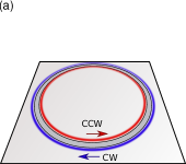
To convey an understanding of how a lasing system with degenerate modes can be described in the SALT framework, let us first consider the well-known example of a rotationally symmetric ring laser whose solution can become unstable in certain parameter regimes Risken and Nummedal (1968); Lugiato et al. (1986); Zeghlache et al. (1988); J.V. Moloney and Newell (1987); Grynberg et al. (1988); Giusfredi et al. (1988); Lugiato et al. (1989); Tureci and Stone (2005); der Sande et al. (2008); Sunada et al. (2011); Kingni et al. (2012). We model the system as a one-dimensional, homogeneous medium with periodic boundary conditions (see Fig. 1a for an illustration). To incorporate losses through absorption and outcoupling, we set the index of refraction to a complex value.

Solving Eq. (6) for the unpumped system produces a set of eigenstates $\{\bar{\omega}_{i},\bar{E}_{i}\}$, where a two-dimensional eigenspace is associated with every eigenvalue $\bar{\omega}_{i}$ due to the rotational symmetry of the system. This eigenspace contains standing waves of the form $e^{i\bar{\omega}_{i}x}\pm\mathrm{c.c.}$ as well as traveling waves of the form $e^{\pm i\bar{\omega}_{i}x}$. While these two pairs of states as well as their superpositions solve Eq. (6) below threshold, the non-linear spatial hole-burning term in the SALT Eq. (4) prevents arbitrary superpositions from being valid solutions above the threshold. This leaves only two possible steady-state lasing solutions of the ringlaser at $\bar{\omega}_{i}$, corresponding to the well known clockwise and counterclockwise traveling wave states. However, from the literature it is known that ring lasers show complex behavior, including the fact that these traveling wave solutions are not always stable Lugiato et al. (1986); Risken and Nummedal (1968); Zeghlache et al. (1988); J.V. Moloney and Newell (1987); Grynberg et al. (1988); Giusfredi et al. (1988); Lugiato et al. (1989); Tureci and Stone (2005); der Sande et al. (2008); Sunada et al. (2011); Kingni et al. (2012).

Our goal here will be to find the single-mode solutions with SALT and to identify the corresponding regions of stability. To approach this problem first in the most general way (i.e., independently of the employed SALT approach), we set up a finite-difference time-domain (FDTD) method based on a Yee lattice Yee (1966); Bidégaray (2003). This tool allows us to solve the MB equations Eq. (1) directly, including the full temporal evolution starting from an initial distribution of the electric field. Using this approach we first confirmed that in the single-mode regime indeed only the traveling modes are stable in certain parameter regimes. To assess the latter, the system was initialized in the traveling-wave solution obtained from the SALT Eq. (4)  and then left to evolve for a certain amount of time. We analyzed whether at later times the system remained in the same steady-state solution as at the beginning of the simulation. If the system stayed in the same state (and did not show any signatures of deviating from this state), we considered the solution to be stable.

Figure 1: (Color online) Results for a one-dimensional ring laser system with circumference $L=1$, $\gamma_{\bot}=1$ and $\omega_{a}=61$. The openness of the system is modeled by a lossy dielectric function $\sqrt{\epsilon(x)}=1+0.0002i$. (a) Sketch of the ring laser system, which can accommodate clockwise (CW) or counterclockwise (CCW) traveling modes. (b) Lasing mode intensity versus applied pump strength for the traveling wave solution. Note that the gain parameters have been chosen such that only a single pair of degenerate modes reaches the lasing threshold. The traveling wave solution in which the system lases has a frequency of $\omega\approx 62.65$ which stays constant while the pump strength is increased. (c) Stability analysis of the SALT results. Shown are the stability of this traveling wave solution under variation of the pump strength $D_{0}$ and the relaxation rate of the inversion $\gamma_{\parallel}$. The results of the FDTD simulation are color-coded with green (light gray) marking parameter combinations where the SALT solution is stable, whereas the red (dark gray) region represents unstable behavior. Blue dashed lines show the independent results of the linear stability analysis, which provides an excellent estimate for the border between stable and unstable regions.

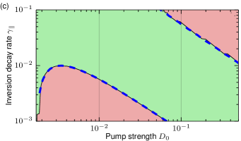
The stability diagram resulting from these FDTD simulations is shown in Fig. 1c. We find that the stability of the single-mode SALT solutions not only depends on the external pump strength $D_{0}$, but also on the inversion decay rate $\gamma_{\parallel}$. This finding concurs with previous results Zeghlache et al. (1988) and shows that while the single-mode SALT solution is an exact solution of the MB equations, it is not necessarily a stable one. For systems with degenerate passive modes (as well as with closely spaced modes $|\Delta\omega|<\gamma_{\parallel}$ discussed below), the stability of any solution obtained from SALT is therefore not guaranteed and needs to be independently verified. Using FDTD for such a verification, as we did above, is, however, much too costly from a numerical point of view, in particular, as this would nullify the computational advantages of SALT. Also the stability analysis presented in Zeghlache et al. (1988) for rotationally symmetric ring lasers is rather limited in scope, as it relies on the availability of exact analytic solutions for the passive modes. We will thus develop below a more general and rigorous framework to analyze the stability of SALT solutions that should be generally applicable.

IV Linear stability analysis

This section contains an overview of a linear stability analysis for solutions of SALT Eq. (4) (a full derivation can be found in appendix A). Our starting point is to linearize the original MB equations (1) around the SALT solution and to assess whether it is stable against small perturbations. In what follows we concentrate on the single-mode solutions only and thus insert the following expressions into the MB equations (1),

$$\begin{split}E(x,t)&=(E_{1}(x)+\delta E(x,t))e^{-i\omega_{1}t},\\ P(x,t)&=(P_{1}(x)+\delta P(x,t))e^{-i\omega_{1}t},\\ D(x,t)&=(D(x)+\delta D(x,t)).\end{split}$$ (9)

In this ansatz, $E_{1}$, $P_{1}$, $D$ denote, respectively, the electric field, the polarization and the inversion of the single-mode SALT solution of Eq. (4) and $\delta E$, $\delta P$, $\delta D$ are the corresponding small perturbations around it. Utilizing the fact that the SALT solution also exactly solves the MB equations and neglecting the higher-order contributions of the perturbations, we derive a set of linear PDEs (13) with respect to $\delta E$, $\delta P$, $\delta D$.

As a next step we convert the resulting system of equations into a standard eigenvalue problem. A split of the complex variables into their imaginary and real parts gives rise to a set of linear equations for five independent fields, which for convenience can be represented as a single vector field, $\vec{F}(x)=(\mathrm{Re}(\delta E),\mathrm{Im}(\delta E),\mathrm{Re}(\delta P),\mathrm{Im}(\delta P),\delta D)$. We look for solutions of the form $\vec{F}(x,t)=\vec{F}(x)e^{\sigma t}$, where $\sigma$ is the growth rate, and derive a set of linear equations (A) containing the spatial dependence only. Using an appropriate discretization scheme and taking into account the periodic boundary conditions, we finally end up with a quadratic eigenvalue problem of the following form:

$$A\vec{F}+\sigma B\vec{F}+\sigma^{2}C\vec{F}=0,$$ (10)

where $A$, $B$ and $C$ are the corresponding matrices whose dimensions depend on the chosen spatial discretization.

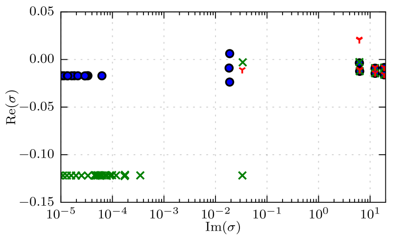
This eigenvalue problem can be solved numerically, resulting in a set of eigenvalues and eigenvectors, $\{\sigma^{j},F^{j}(x)\}$. Note that eigenvalues with $\text{Re}(\sigma^{j})>0$ stand for the perturbations, which grow exponentially in time implying that our SALT solution is unstable. Conversely, if all eigenvalues $\sigma^{j}$ have a real part smaller than zero, the SALT solution is stable against small perturbations. Therefore, finding the eigenvalue with the largest real part is sufficient to classify the stability of the SALT solution. The imaginary part of $\sigma$ stands for the frequency relative to $\omega_{1}$, with which the perturbation oscillates. In Fig. 2, we show a typical example of the eigenvalue spectra $\{\sigma^{j}\}$ with different values of $\gamma_{\parallel}$ for the case of the symmetric ring laser described in the previous section. Note that due to the fact that the MB equations for the single-mode regime are invariant under a global phase rotation, the value $\sigma=0$ always shows up. It, however, does not affect the behavior of the system and therefore is always excluded from the consideration.

To assess the stability diagram of a SALT solution we start at a certain value of the pump strength and then gradually vary the value of $\gamma_{\parallel}$. The dashed lines in the stability diagram depicted in Fig. 1c correspond to the stability thresholds at which the eigenvalue with the largest real part, $\max_{j}[\mathrm{Re}(\sigma^{j})]$, crosses the imaginary axis [$\mathrm{Re}(\sigma)=0$]. We emphasize that the boundaries between stable and unstable regions, which we find in this way, are in excellent agreement with the time-dependent simulations, as seen in Fig. 1c. It should be noted that previous studies on such a linear stability analysis involved more restrictive approximations and a limited class of perturbations by keeping track of low order Fourier terms only Zeghlache et al. (1988), whereas our approach is exact in the framework of the MB equations.

Note, that for the above procedure to work it is not necessary to compute the whole eigenvalue spectrum $\{\sigma^{j}\}$, but it is sufficient to only consider eigenvalues in the complex region close to the real axis and for imaginary parts in the range of $0$ to $\omega_{1}$. In systems where the rotating wave approximation is justified, only perturbations within this frequency range can realistically influence the system. In systems with a complex refractive index, spurious solutions that need to be excluded from the analysis, can occur in the region $|\mathrm{Im}(\sigma)|>\omega_{1}$. This restriction on the eigenvalues we are looking for can be used together with an iterative eigenvalue solver to check relatively quickly if a solution is stable or not Saad (1992).

It is worth noting that for the above stability analysis of the MB equations no additional assumptions have been made and the results are therefore valid for arbitrary single-mode SALT solutions. In the next section we consider the ring laser with an embedded scatterer where modes are only near-degenerate to see how our results change for the case of such a slight lift of the degeneracy.

Figure 2: (Color online) Stability eigenvalues $\sigma^{j}$ of the ring laser for $D_{0}=0.06$ and $\gamma_{\parallel}=10^{-3}$ (blue circles), $\gamma_{\parallel}\approx 7\cdot 10^{-3}$ (green crosses) and $\gamma_{\parallel}=10^{-1}$ (red Ys). All other parameters are chosen as in Fig. 1. One can see that the single-mode lasing solution is only stable for the intermediary value of $\gamma_{\parallel}$ (green crosses), since for both other cases, a $\sigma^{j}$ with a real part larger than zero exists. The stability eigenvalues with $\mathrm{Im}(\sigma^{i})\approx 10^{-2}$ are related to the competition between the nearly degenerate modes. The other visible clusters of stability eigenvalues at $\mathrm{Re}(\sigma^{i})\approx-\gamma_{\parallel}$ are related to damped relaxation oscillations observed when initially turning on the laser. The eigenvalues with $\mathrm{Im}(\sigma^{j})>10$ are related to other resonances of the system that could potentially also turn into active lasing modes.

V Example 2: 1D ring laser with broken symmetry

In any real-world implementation of a ring laser or microdisk laser, the rotational symmetry will be slightly broken due to inhomogeneities in the material or by imperfections of the manufacturing process Liew et al. (2014a, b). While intuitively one would expect that a slight modification of the system should not change the structure of the lasing solutions, there is evidence that this symmetry breaking can have a strong effect on the lasing modes Liew et al. (2014b); Wiersig (2011). In order to better understand the impact of such a slight symmetry breaking on the stability of the SALT solutions, we analyze here a ring laser where the rotational symmetry is broken by a scatterer as depicted in Fig. 3a.

Since the inhomogeneity in this system breaks the rotational symmetry, solving Eq. (6) for the inactive system will not produce any traveling wave solutions. Instead, standing wave solutions similar to those found in the completely symmetric system are found. But while the standing wave solutions of the symmetric system always occurred in degenerate pairs, breaking the symmetry lifts the degeneracy such that the new modes slightly differ in their complex frequencies $\bar{\omega}_{i}$. Therefore, they will neither possess exactly the same lasing frequency, nor will they reach the lasing threshold at exactly the same same pump strength $D_{0}$. Since the frequency splitting does not fulfill the stationary inversion approximation for realistic values of $\gamma_{\parallel}$, a possible two-mode solution can not be described by SALT (at least not without an explicit stability analysis).

Figure 3: (Color online) Results for a ring laser system as in Fig. 1 with $\gamma_{\parallel}=0.01$, but with an additional scatterer added with $l=0.05$ and $\sqrt{\epsilon}=1.05+0.0002i$. (a) Sketch of the system. (b) Frequencies of single-mode SALT solutions. It can be seen that the two degenerate modes of the symmetric system from Fig. 1 have split into modes $A$ and $B$. Additionally, at $D_{0}\approx 0.003$, two predominantly traveling wave solutions $C_{1}$ and $C_{2}$ branch off from solution $A$. These two solutions are mirror-symmetric images of each other. Dotted lines mark unstable, solid lines mark stable solutions. (c) Intensity distribution of modes $A$ and $C_{1}$ with the scatterer marked in gray. Mode $A$ is shown directly at threshold ($D_{0}\approx 0.0015$), mode $C_{1}$ at $D_{0}=0.1$. It can be seen that while $A$ is a standing wave with minimal intensity $0$ at the nodes, the predominantly traveling wave $C_{1}$ features a non-vanishing intensity everywhere in the cavity. The stability of mode $C_{1,2}$ is studied in Fig. 4.

Figure 4: (Color online) Stability of the SALT solution for the broken symmetry ring laser shown in Fig. 3. The analyzed solution is the one marked as branch $C_{1,2}$ in Fig. 3b. While the shape of the stability region is very similar to the one observed in Fig. 1, the broken symmetry system requires a minimal pump strength $D_{0}$ to compensate for the frequency splitting of the nearly degenerate modes before a stable predominantly traveling wave solution can emerge.

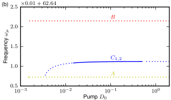
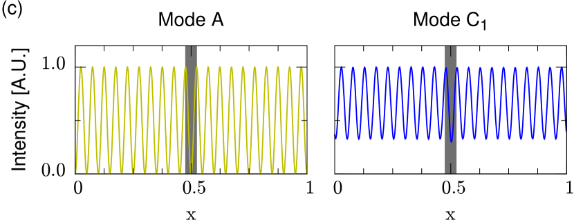
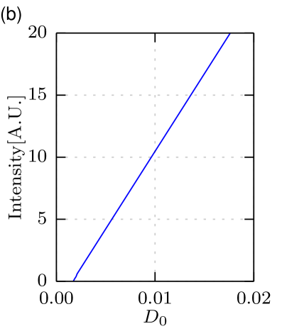
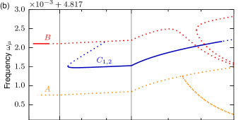
In our analysis we consider gain parameters that only support the lasing action of a single pair of such modes (here located at $\bar{\omega}_{i}\approx 62$) such that only the single-mode solutions of SALT seem viable candidates for steady-state lasing. These single-mode SALT solutions are shown in Fig. 3b in form of their frequency dependence on the pump strength $D_{0}$. In particular, the two single-mode solutions of SALT corresponding to the pair of nearly degenerate resonator modes are shown as mode $A$ and $B$. When tracking mode $A$ from its threshold while increasing the pump strength, it shows the following behavior: At $D_{0}\approx 0.0015$ the standing wave single-mode solution $A$ becomes active and the system starts lasing (see Fig. 3b). At this pump value the mode is stable, both according to the traditional SALT criterion for stability as well as in the linear stability calculations. However, a very small increase of the pump strength brings the eigenvalue $\bar{\omega}_{i}$ of the second mode of this near-degenerate pair to the real axis and thus renders the single-mode solution unstable (again, according to both criteria). Whether a stable two-mode solution in this near-degenerate regime exists is a question that presently falls outside the scope of SALT (due to the non-stationary inversion)Burkhardt (2015). However, with the techniques presented above we can investigate the stability of a single-mode solution in the regime beyond the point where the second mode passes the instability threshold. For this purpose, we track each of the two modes $A$ and $B$ towards higher pump strength using the SALT equation Eq. (4) for each mode as if the other mode was not active. Using, in addition, the stability criterion from the previous section reveals that both solutions on their own remain unstable for higher values of the pump strength. We find, however, that a bifurcation occurs at $D_{0}\approx 0.003$, at which two further single-mode SALT solutions $C_{1,2}$ of Eq. (4) branch off from solution $A$. These new modes share the same frequency, which lies approximately in between the frequencies of the unstable modes $A$ and $B$. To find these two modes one can, e.g., use a linear superposition of mode $A$ and $B$ at higher pump strengths as an initial guess for solving Eq. (4), similarly to the way the traveling wave solutions of the symmetric ring laser can be expressed as linear superpositions of the standing wave solutions.

By looking at the mode profiles of solutions $C_{1,2}$ ($C_{1}$ is shown in Fig. 3c), we observe that these modes are related to the traveling wave solutions observed in the system with unbroken rotational symmetry. There, the two stable solutions were purely clockwise or counter-clockwise traveling waves. Here, each of the modes $C_{1,2}$ still features a dominant contribution in one direction and is identical to the other mode when being reflected at the symmetry axis containing the scatterer ($x=0.5$). The major difference to the solutions observed in the unbroken ring laser is that the solutions $C_{1,2}$ do not exist below a critical pump strength $D_{\mathrm{crit}}\approx 0.003$, since the nonlinear term in Eq. (4) needs to be strong enough to compensate for the frequency splitting between the two modes. The fact that the nonlinear term is responsible for compensating the frequency difference between the two nearly degenerate modes was further investigated. We used a linear approximation to estimate the frequency shift experienced by the passive mode of the system that corresponds to the single-mode solution $B$ as a consequence of the spatial hole burning from the active mode $A$. For this purpose, we modeled the change in the population inversion $\Delta D(x)$ as well as the resulting change in frequency $\Delta\bar{\omega}_{B}$ of the passive mode as a linear function of the pump strength $D_{0}$. The estimate predicted the two modes to share their frequency at a value of $D_{0}\approx 0.30$, which is very close to the point $D_{0}\approx 0.33$, where the solutions $C_{1,2}$ really emerge. The remaining small discrepancy can be attributed to the inaccuracy of the employed approximations.

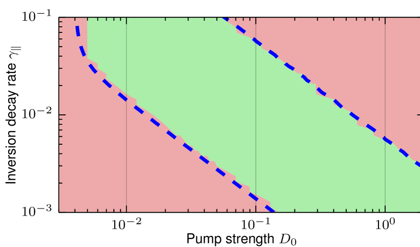
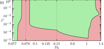
Next, we check the stability of the mode pair $C_{1,2}$. First of all we recall that using the traditional SALT criterion Eq. (8) (which is not applicable here), one would find that the solutions $C_{1,2}$ are never stable. However, both the results of the FDTD calculations as well as the linear stability calculations do show that these modes are stable in well-defined limits. These limits are indicated in Fig. 4, where the stability of the single-mode solutions are depicted as obtained from both methods under variation of the pump strength $D_{0}$ as well as of the relaxation rate of the inversion $\gamma_{\parallel}$. As discussed in the above paragraph, there is a small region of stability for very low values of pump strength $D_{0}$ where mode $A$ is stable. Of more interest, however, is the large region of stable lasing for modes $C_{1,2}$ which opens up at the critical pump strength $D_{\mathrm{crit}}\approx 0.003$ (green region in Fig. 4) and which is similar to the one observed for the fully symmetric ring laser (Fig. 1).

Altogether, the results of the linear stability analysis are in excellent agreement with the findings of the time-dependent simulations of the MB equations, as can be seen both in Fig. 1b and in Fig. 4. The linear stability analysis thus proves to be a reliable tool to classify the stability of SALT solutions and can therefore be used even for systems where verifying the results through time-dependent simulations is not feasible. This is, in particular, the case for higher dimensional systems, such as the microdisk system analyzed in the next section, where time-dependent simulations for a large range of parameters is computationally very demanding.

VI Example 3: 2D microdisk laser with wedge

Figure 5: (Color online) Single-mode lasing states for a 2D cavity with a wedge. The disk has a radius of $1$, a refractive index of $n=2+0.01i$ and the wedge on the right side of the disk has a depth of $0.05$ and a width of $0.05$. The gain parameters are $\omega_{a}=4.83$ and $\gamma_{\bot}=0.1$. (a) The cavity is outlined in white with arrows marking the position of the wedge. The spatial intensity pattern of two stable single-mode solutions are shown: (left) Standing wave mode $B$ at pump strength $D_{0}=0.0773$ with regularly spaced nodes with intensity zero; (right) dominantly traveling wave solution $C_{1}$ at pump strength $D_{0}=0.15$. (b) Laser frequencies of single-mode solutions to the SALT Eq. (4). Curves $A$ (orange) and $B$ (red) correspond to two standing wave solutions, which have even and odd symmetry with respect to the $x$-axis. The two modes represented by curve $C_{1,2}$ (blue) feature a broken symmetry, but are mirror-symmetric to each other. Solid (dotted) lines denote a stable (unstable) solution for $\gamma_{\parallel}=0.01$. Note, that the pump axis is separated into three regions of different linear scaling for the sake of clarity. (c) Stability diagram of the single-mode solutions shown in (b) with respect to the pump strength $D_{0}$ and the relaxation rate of the inversion, $\gamma_{\parallel}$. The color-coding is as in Fig. 1c except that the stability is here solely determined by the linear stability analysis.

Next, we will extend our results to a two-dimensional system, where full time-dependent simulations become impractical for the required range of parameters, but the linear stability analysis can still be easily performed to justify the stability of the SALT solutions. The system we will consider is a perturbed 2D microdisk laser where the cavity is slightly deformed by cutting a small wedge into the disk (see arrow and white outline in Fig. 5a). In analogy to the scatterer for the 1D ring laser, the wedge has the effect that the two originally degenerate threshold modes of the microdisk split (here the frequency splitting $\Delta\omega\approx 1.4\cdot 10^{-3}$). Hence, the multi-mode condition $\gamma_{\parallel}\ll\Delta\omega$ cannot be satisfied for reasonable values of $\gamma_{\parallel}$ such that a two mode solution does not fulfill the SIA and the traditional SALT algorithm cannot be applied.

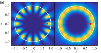
The strategy to find the single-mode SALT solutions is a bit more sophisticated as compared to the 1D system. We start with the threshold modes $A$ and $B$ corresponding to the nearly degenerate resonances of the unpumped system and track them while gradually increasing the pump strength $D_{0}$ (see Fig. 5b). Mode $B$ has a lower threshold and is stable in a tiny pump region starting from its threshold at $D_{0}\approx 0.0771$ up to about $0.0777$. The corresponding stable parameter region for mode $B$, shown in the stability diagram in Fig. 5c by the green region on the very left of the figure, depends on both the pump strength $D_{0}$ and on $\gamma_{\parallel}$. After mode $B$ has become unstable the mode is tracked further (neglecting the presence of mode $A$ whose resonance eigenvalue has meanwhile also crossed the real axis). At $D_{0}\approx 0.124$ a pair of solutions $C_{1,2}$ branches off from mode $B$. Whereas mode $B$ and mode $A$ feature a perfect even and odd symmetry with respect to the $x$-axis (i.e., the symmetry axis of the system), the solutions $C_{1,2}$ do not possess this symmetry, but rather are mirror images of each other (compare mode profiles of modes $B$ and $C_{1}$ in Fig. 5a). In fact, the symmetry of the system is spontaneously broken when either of these modes are lasing, a phenomenon that has been previously observed in simulations as well as in experiments Harayama et al. (2003).

In contrast to mode $B$, mode $A$ is never a stable laser mode since it has a higher lasing threshold. At $D_{0}\approx 0.8$ both (unstable) modes $A$ and $B$ feature two further branches. These can be understood as follows: Since the wedge of the two dimensional cavity only represents a small perturbation to the system, the symmetry with respect to the $y$-axis is only slightly broken, and, hence, modes $A$ and $B$ are nearly symmetric with respect to this axis (see left panel of Fig. 5a for the intensity pattern of mode $B$). At $D_{0}\approx 0.8$, this near-symmetry is no longer realized. However, since the modes have never been fully symmetric, there is not a single point at which the symmetry breaks, but rather a smooth transition (as compared, e.g., to the symmetry breaking transition with respect to the $x$-axis at $D_{0}\approx 0.124$). For mode $B$, this smooth transition is clearly visible in Fig. 5b. For mode $A$ this transition occurs in a much smaller pump interval, since mode $A$ has a node directly located at the wedge of the 2D cavity and its symmetry is therefore only very slightly distorted.

To obtain modes $C_{1,2}$, we need to track them backwards in pump strength starting at the branching point at $D_{0}\approx 0.124$ (see Fig. 5b). Reducing the pump strength further, we observe that a sharp bend occurs in the frequency dependence of these two modes at $D_{0}\approx 0.86$, where each of the modes $C_{1,2}$ has evolved into a dominantly traveling wave mode (see right panel of Fig. 5a), similar to the nearly degenerate 1D ring laser. Note that the small contribution traveling in clockwise direction can be observed as a modulation in the intensity pattern. Beyond this turning point, modes $C_{1,2}$ become stable in a large region of parameters $D_{0}$ and $\gamma_{\parallel}$ as depicted by the central green area in the stability diagram in Fig. 5c. The easiest way to find the branch $C_{1,2}$ numerically is to sum the fields of modes $A$ and $B$ with an additional relative phase of $\pi/2$ at a pump strength $D_{0}>0.86$ and use this as a guess for the nonlinear solver to converge towards one of the dominantly traveling wave modes. The solution can then be tracked to uncover the whole branch of modes $C_{1,2}$. Using similar superpositions of already known modes as starting point for the nonlinear solver, we found several more branches of non-linearly induced single-mode SALT solutions within the plotted frequency range, albeit none of them are stable (these branches are not shown in Fig. 5c).

The traveling wave solutions $C_{1,2}$ only remain stable until a pump strength of $D_{0}\approx 1.3$. Here, the single-mode SALT solution becomes unstable due to the fact that an additional mode would start to lase. We also find that for values of $\gamma_{\parallel}<2\cdot 10^{-5}$ the modes $C_{1,2}$ are never stable, which highlights again how important it is to take into account the value of $\gamma_{\parallel}$ for assessing the stability of a SALT mode. Traditionally in SALT single-mode lasing solutions were implicitly considered as stable (without considering $\gamma_{\parallel}$) Türeci et al. (2006); Esterhazy et al. (2014), but these single-mode solutions were always only identified for the case where only a single one of the eigenvalues $\bar{\omega}_{i}$ of Eq. (7) has a non-negative imaginary part. Our results show that single-mode SALT solutions can also exist for the case of multiple eigenvalues $\bar{\omega}_{i}$ featuring a non-negative imaginary part. In this new situation, a stability analysis is, however, indispensable for correctly interpreting the solutions of the SALT equation. When the results of the stability analysis are taken into account, the SALT equation allows us to accurately describe the steady-state of these systems without requiring any time-dependent simulations.

VII Conclusion

In this work we demonstrate that SALT can be used to describe the single-mode lasing regime of resonators with degenerate or near-degenerate mode pairs. Our approach builds on a careful tracking of SALT modes in the non-linear lasing regime together with a linear stability analysis to judge the validity of the resulting solutions. The accuracy of the stability analysis itself was tested by a comparison with full time-dependent simulations based on the Maxwell-Bloch equations, which shows excellent agreement in all cases.

Our approach is ideally suited to treat microdisk whispering-gallery-mode lasers, which were previously difficult to simulate with SALT and often only accessible through time-dependent simulations or through strongly simplified models. Generally speaking, our work paves the way to study interesting non-linear phenomena, such as bifurcating solutions etc. within the efficient framework of SALT.

One obvious direction for further study is the generalization of our stability analysis to systems in the multi-mode lasing regime, which will be the aim of a subsequent paper Burkhardt (2015).

VIII Acknowledgments

*

Appendix A Appendix A: Derivation of the linear stability analysis

We start from a solution $\{E_{1}(x),\omega_{1}\}$ of the SALT Eq. (4) at a given pump strength $D_{0}$. From this, one can construct the polarization, $P_{1}$, and inversion, $D$, that show up in the MB Eqs. (4) via

$$D(x) = \frac{D_{0}}{1+|\Gamma_{1}E_{1}(x)|^{2}}$$ (11)

$$P_{1}(x) = \Gamma_{1}D(x)E_{1}(x).$$ (12)

Using these quantities, we insert the ansatz (9) into the MB Eqs. 1. Using the fact that $(E_{1}e^{-i\omega_{1}t},P_{1}e^{-i\omega_{1}t},D)$ is a solution of the MB equations, we linearize the equations with respect to the perturbations. This results in the following partial differential equations for the perturbations of the electric field, the polarization, and the inversion

$$\epsilon\,\delta\ddot{E}= \nabla^{2}\delta E-\delta\ddot{P}+\omega_{1}^{2}(\delta P+\epsilon\,\delta E)\,+2i\omega_{1}(\delta\dot{P}+\epsilon\,\delta\dot{E})$$ (13)

$$\delta\dot{P}= \left(i(\omega_{1}-\omega_{a})-\gamma_{\bot}\right)\delta P-i\gamma_{\bot}(E\,\delta D+\delta E\,D)$$ (14)

$$\delta\dot{D}= -\gamma_{\parallel}\,\delta D+\frac{i\gamma_{\parallel}}{2}\big{(}\delta E\,P_{1}^{*}+E_{1}\,\delta P^{*}-\delta E^{*}P_{1}-E_{1}^{*}\,\delta P\big{)}.$$ (15)

While this system of equations is linear in the perturbation, it includes the terms $\delta P^{*}$ and $\delta E^{*}$, which can not be expressed as linear combination of $\delta P,\delta E,\delta D$. In order to produce a completely linear system of equations, we therefore split the two complex fields and corresponding perturbations, as well as a possibly complex dielectric function $\varepsilon$ into their respective real and imaginary parts and consequently split Eqs. (13) and (14) into four real equations. This yields a linear system of five equations with purely real terms. These correspond to the five independent fields $\mathrm{Re}(\delta E)$, $\mathrm{Im}(\delta E)$, $\mathrm{Re}(\delta P)$, $\mathrm{Im}(\delta P)$, $\delta D$, which for convenience we can summarize as a single vector field $\vec{F}$.

In order to analyze if a solution $E_{1}$ of the SALT equation (4) is stable we need to check if a perturbation exists which doesn’t relax back to the stable solution. Hence, we make an ansatz of the form $\vec{F}(x,t)=\vec{F}(x)e^{\sigma t}$ which yields

$$(\delta P_{r}-\epsilon_{i}\delta E_{i}+\epsilon_{r}\delta E_{r})\sigma^{2}+2(\delta P_{i}+\epsilon_{i}\delta E_{r}+\epsilon_{r}\delta E_{i})\omega_{1}\,\sigma-(\delta P_{r}-\epsilon_{i}\delta E_{i}+\epsilon_{r}\delta E_{r})\,\omega_{1}^{2}-\nabla^{2}\delta E_{r} =0$$

$$(\delta P_{i}+\epsilon_{i}\delta E_{r}+\epsilon_{r}\delta E_{i})\sigma^{2}-2(\delta P_{r}-\epsilon_{i}\delta E_{i}+\epsilon_{r}\delta E_{r})\omega_{1}\sigma-(\delta P_{i}+\epsilon_{i}\delta E_{r}+\epsilon_{r}\delta E_{i})\omega_{1}^{2}-\nabla^{2}\delta E_{i} =0$$

$$\delta P_{r}\sigma+\gamma_{\bot}(\delta P_{r}-D\delta E_{i}-\delta DE_{i}^{1})+(\omega_{1}-\omega_{a})\delta P_{i} =0$$ (16)

$$\delta P_{i}\sigma+\gamma_{\bot}(\delta P_{i}+D\delta E_{r}+\delta DE_{r}^{1})-(\omega_{1}-\omega_{a})\delta P_{r} =0$$

$$\delta D\sigma+\gamma_{\parallel}(\delta D+P_{r}^{1}\delta E_{i}+\delta P_{r}E_{i}^{1}-\delta E_{r}P_{i}^{1}-E_{r}^{1}\delta P_{i}) \,=0,$$

where we have abbreviated $\text{Re}(\cdot)$ and $\text{Im}(\cdot)$ through the sub-indices $r$ and $i$, respectively. In addition we need to impose boundary conditions for the perturbation $\delta E$. For the periodic 1D ring laser we can simply assume periodic boundary conditions, i.e., $\delta E(x_{\text{left}})=\delta E(x_{\text{right}})$ and for the 2D system $\vec{\nabla}\delta E\overset{r\to\infty}{=}i(\omega_{1}-i\sigma)\delta E\,\hat{e}_{r}$. In a next step Eqs. (16) are discretized using a suitable discretization scheme Esterhazy et al. (2014) which leads to a quadratic eigenvalue problem that can easily be linearized. In our calculations we have chosen the finite element framework FEniCS Logg et al. (2012) for discretizing Eqs. (16) and used a perfectly matched layer for imposing the outgoing boundary conditions in the 2D case. For solving the linearized quadratic eigenvalue problem we have used SLEPc Hernandez et al. (2005).

References

- Vahala (2003) K. J. Vahala, Nature 424, 839 (2003).
- Cao and Wiersig (2015) H. Cao and J. Wiersig, Rev. Mod. Phys. 87, 61 (2015).
- Nöckel and Stone (1997) J. U. Nöckel and A. D. Stone, Nature 385, 45 (1997).
- Gmachl et al. (1998) C. Gmachl, F. Capasso, E. E. Narimanov, J. U. Nöckel, A. D. Stone, J. Faist, D. L. Sivco, and A. Y. Cho, Science 280, 1556 (1998).
- Harayama et al. (2003) T. Harayama, T. Fukushima, S. Sunada, and K. S. Ikeda, Phys. Rev. Lett. 91, 073903 (2003).
- Lebental et al. (2006) M. Lebental, J. S. Lauret, R. Hierle, and J. Zyss, Applied Physics Letters 88, 031108 (2006).
- Song et al. (2009) Q. Song, W. Fang, B. Liu, S.-T. Ho, G. S. Solomon, and H. Cao, Phys. Rev. A 80, 041807 (2009).
- Wang et al. (2010) Q. J. Wang, C. Yan, N. Yu, J. Unterhinninghofen, J. Wiersig, C. Pflügl, L. Diehl, T. Edamura, M. Yamanishi, H. Kan, and F. Capasso, PNAS 107, 22407 (2010).
- Yang et al. (2010) J. Yang, S.-B. Lee, S. Moon, S.-Y. Lee, S. W. Kim, T. T. A. Dao, J.-H. Lee, and K. An, Phys. Rev. Lett. 104, 243601 (2010).
- Albert et al. (2012) F. Albert, C. Hopfmann, A. Eberspächer, F. Arnold, M. Emmerling, C. Schneider, S. Höfling, A. Forchel, M. Kamp, J. Wiersig, and S. Reitzenstein, Applied Physics Letters 101, 021116 (2012).
- Peng et al. (2014) B. Peng, Ş. K. Özdemir, S. Rotter, H. Yilmaz, M. Liertzer, F. Monifi, C. M. Bender, F. Nori, and L. Yang, Science 346, 328 (2014).
- Brandstetter et al. (2014) M. Brandstetter, M. Liertzer, C. Deutsch, P. Klang, J. Schöberl, H. E. Türeci, G. Strasser, K. Unterrainer, and S. Rotter, Nat Commun 5, 4034 (2014).
- Haken and Sauermann (1963) H. Haken and H. Sauermann, Zeitschrift für Physik 173, 261 (1963).
- Lamb (1964) W. E. Lamb, Phys. Rev. 134, A1429 (1964).
- Lang et al. (1973) R. Lang, M. O. Scully, and W. E. Lamb, Phys. Rev. A 7, 1788 (1973).
- Haken (1986) H. Haken, Laser Light Dynamics, Volume II (North Holland, 1986).
- Türeci et al. (2006) H. E. Türeci, A. D. Stone, and B. Collier, Phys. Rev. A 74, 043822 (2006).
- Ge et al. (2008) L. Ge, R. J. Tandy, A. D. Stone, and H. E. Türeci, Opt. Express 16, 16895 (2008).
- Türeci et al. (2009) H. E. Türeci, A. D. Stone, L. Ge, S. Rotter, and R. J. Tandy, Nonlinearity 22, C1 (2009).
- Ge et al. (2010) L. Ge, Y. D. Chong, and A. D. Stone, Phys. Rev. A 82, 063824 (2010).
- Cerjan and Stone (2014) A. Cerjan and A. D. Stone, Phys. Rev. A 90, 013840 (2014).
- Esterhazy et al. (2014) S. Esterhazy, D. Liu, M. Liertzer, A. Cerjan, L. Ge, K. G. Makris, A. D. Stone, J. M. Melenk, S. G. Johnson, and S. Rotter, Phys. Rev. A 90, 023816 (2014).
- Pick et al. (2015) A. Pick, A. Cerjan, D. Liu, A. W. Rodriguez, A. D. Stone, Y. D. Chong, and S. G. Johnson, ArXiv e-prints (2015), arXiv:1502.07268 [physics.optics] .
- Türeci et al. (2008) H. E. Türeci, L. Ge, S. Rotter, and A. D. Stone, Science 320, 643 (2008).
- Liertzer et al. (2012) M. Liertzer, L. Ge, A. Cerjan, A. D. Stone, H. E. Türeci, and S. Rotter, Phys. Rev. Lett. 108, 173901 (2012).
- Chitsazi et al. (2014) M. Chitsazi, S. Factor, J. Schindler, H. Ramezani, F. M. Ellis, and T. Kottos, Phys. Rev. A 89, 043842 (2014).
- Chong et al. (2010) Y. D. Chong, L. Ge, H. Cao, and A. D. Stone, Phys. Rev. Lett. 105, 053901 (2010).
- Wan et al. (2011) W. Wan, Y. Chong, L. Ge, H. Noh, A. D. Stone, and H. Cao, Science 331, 889 (2011).
- Hisch et al. (2013) T. Hisch, M. Liertzer, D. Pogany, F. Mintert, and S. Rotter, Phys. Rev. Lett. 111, 023902 (2013).
- Liew et al. (2014a) S. F. Liew, B. Redding, L. Ge, G. S. Solomon, and H. Cao, Applied Physics Letters 104, 231108 (2014a).
- Gagnon et al. (2014) D. Gagnon, J. Dumont, J.-L. Déziel, and L. J. Dubé, J. Opt. Soc. Am. B 31, 1867 (2014).
- Zeghlache et al. (1988) H. Zeghlache, P. Mandel, N. B. Abraham, L. M. Hoffer, G. L. Lippi, and T. Mello, Phys. Rev. A 37, 470 (1988).
- Risken and Nummedal (1968) H. Risken and K. Nummedal, Physics Letters A 26, 275 (1968).
- Chua et al. (2011) S.-L. Chua, Y. Chong, A. D. Stone, M. Soljacic, and J. Bravo-Abad, Opt. Express 19, 1539 (2011).
- Cerjan et al. (2012) A. Cerjan, Y. Chong, L. Ge, and A. D. Stone, Opt. Express 20, 474 (2012).
- Note (1) The restriction to TM modes is only due to the fact that this simplifies the equations. However, the results presented in this work equally apply if one uses the full three-dimensional MB, where are vector quantities.
- Berenger (1994) J.-P. Berenger, Journal of Computational Physics 114, 185 (1994).
- Note (2) As discussed in Esterhazy et al. (2014) further conditions come into play for the “bad cavity limit”, which, however, we do not consider for the systems shown in this paper.
- Burkhardt (2015) S. Burkhardt, to be submitted (2015).
- Lugiato et al. (1986) L. A. Lugiato, L. M. Narducci, and M. F. Squicciarini, Phys. Rev. A 34, 3101 (1986).
- J.V. Moloney and Newell (1987) D. M. J.V. Moloney, H. Adachihara and A. Newell, in Chaos, Noise and Fractals, Malvern Physics Series, edited by E. Pike and L. Lugiato (Taylor & Francis, 1987) pp. 137–187.
- Grynberg et al. (1988) G. Grynberg, E. L. Bihan, P. Verkerk, P. Simoneau, J. Leite, D. Bloch, S. L. Boiteux, and M. Ducloy, Optics Communications 67, 363 (1988).
- Giusfredi et al. (1988) G. Giusfredi, J. F. Valley, R. Pon, G. Khitrova, and H. M. Gibbs, J. Opt. Soc. Am. B 5, 1181 (1988).
- Lugiato et al. (1989) L. Lugiato, F. Prati, L. Narducci, and G.-L. Oppo, Optics Communications 69, 387 (1989).
- Tureci and Stone (2005) H. E. Tureci and A. D. Stone, “Mode competition and output power in regular and chaotic dielectric cavity lasers,” (2005).
- der Sande et al. (2008) G. V. der Sande, L. Gelens, P. Tassin, A. Scirè, and J. Danckaert, Journal of Physics B: Atomic, Molecular and Optical Physics 41, 095402 (2008).
- Sunada et al. (2011) S. Sunada, T. Harayama, K. Arai, K. Yoshimura, K. Tsuzuki, A. Uchida, and P. Davis, Opt. Express 19, 7439 (2011).
- Kingni et al. (2012) S. T. Kingni, G. V. der Sande, L. Gelens, T. Erneux, and J. Danckaert, J. Opt. Soc. Am. B 29, 1983 (2012).
- Yee (1966) K. Yee, Antennas and Propagation, IEEE Transactions on 14, 302 (1966).
- Bidégaray (2003) B. Bidégaray, Numerical Methods for Partial Differential Equations 19, 284 (2003).
- Note (3) We alternatively analyzed the situation when the simulation was not initialized in the state obtained from the SALT solution but in an arbitrary initial state instead. If the parameters of the system were such that the SALT solution was stable (see Fig. 1), the system would usually converge to the SALT solution over time. In the region close to the border between stable and unstable solution, the system only converged to the SALT solution for certain initial conditions, hinting at the existence of a second stable non-steady-state solution.
- Saad (1992) Y. Saad, Numerical Methods for Large Eigenvalue Problems (Halsted Press, New York, NY, 1992).
- Liew et al. (2014b) S. F. Liew, L. Ge, B. Redding, G. S. Solomon, and H. Cao, arXiv:1412.8513 [physics] (2014b), arXiv: 1412.8513.
- Wiersig (2011) J. Wiersig, Phys. Rev. A 84, 063828 (2011).
- Logg et al. (2012) A. Logg, K.-A. Mardal, and G. Wells, eds., Automated Solution of Differential Equations by the Finite Element Method, Lecture Notes in Computational Science and Engineering, Vol. 84 (Springer, Berlin Heidelberg, 2012).
- Hernandez et al. (2005) V. Hernandez, J. E. Roman, and V. Vidal, ACM Trans. Math. Softw. 31, 351 (2005).