Distributed Computation Particle PHD filter

Abstract

Particle probability hypothesis density filtering has become a promising means for multi-target tracking due to its capability of handling an unknown and time-varying number of targets in non-linear non-Gaussian system. However, its computational complexity grows linearly with the number of measurements and particles assigned to each target, and this can be very time consuming especially when numerous targets and clutter exist in the surveillance region. Addressing this issue, we present a distributed computation particle PHD filter for target tracking. Its framework consists of several local particle PHD filters at each processing element and a central unit. Each processing element takes responsibility for part particles but full measurements and provides local estimates; central unit controls particle exchange between processing elements and specifies a fusion rule to match and fuse the estimates from different local filters. The proposed framework is suitable for parallel implementation and maintains the tracking accuracy. Simulations verify the proposed method can provide comparative accuracy as well as a significant speedup with the standard particle PHD filter.

1 Introduction

Multi-target tracking(MTT) is to jointly estimate the number of targets and position from a set of uncertain observations. The classical approaches such as the nearest neighbor(NN)[10],Joint Probabilistic Data Association filter(JPDA)[6], and Multi-hypothesis tracking(MHT)[4] are based on the association algorithms.

Recently,much work has devoted to random finite set(RFS)-based approximations such as the probability hypothesis density(PHD)[7],[12],cardinalised PHD(CPHD)[8] [2] and multiple target multi-Bernoulli(MeMBer) filter[3].These methods avoid the data association problem. From implementation perspective, a particle PHD filter for nonlinear non-Gaussian MTT problems,was proposed in [1]. And Vo [12] proposed a close-form solution to PHD filter with assumptions on linear Gaussian system. It is called GM-PHD filter.

The demands of "real-time" MTT have been growing. Since the CPHD filter propagates both the intensity of the RFS and the posterior cardinality distribution,its real time characteristic is intrinsically not as good as the PHD filter.The MeMBer filter is more suitable for low clutter environments.And the GM-PHD is constrained to linear Gaussian system. The particle PHD filter is more suitable for nonlinear non-Gaussian MTT problems in dense clutter environment.However,the particle PHD filter computational complexity is very high,Therefore,we are interested in improving the real-time performance of the particle PHD filter.

Similar to the particle filter,the resampling is chief obstacles to parallel and distribute. [5] had proposed the distributed particle resampling algorithm and implement in many WSN applications.In this paper,we proposed a distributed particle PHD filter. In order to apply particle PHD filter theory to practice,distributed algorithm is better than centralized algorithm. Since the distributed algorithm can reduce the execution time by implementing the particle PHD filter using multiple processing elements. We distribute the particles to N PEs.Each PE can run particle PHD filter independently.All individual PEs compute local estimates based over observations in parallel,and transmit their estimate to a CU to obtain global estimate.

Moreover,if the PEs were let to run as independent particle PHD filter,each of them most likely have performance degradation caused by part of particles.The particles exchange will solve the problem.

The main contribution of this paper is summarized as follows. First,we proposed the distributed particle PHD filter architecture. Second,we use the stphd method to extract the state estimation and corresponding measurement label.

The real time performance is enhanced and the tracking performance is equal to traditional particle PHD filter.

The remainder of this paper is organized as follows, standard particle PHD filter is given in section 2.Section 3 ,we present our distributed particle PHD filter in detail.Simulation results are given in Section 4.Section 5 is devoted to the conclusions.

2 Backgroud

2.1 The PHD FILTER

The PHD filter was developed in the framework of Finite Set Statistics(FISST) initially. The PHD function $D_{\Xi}$ is the first order moment of the random finite set(RFS) $\Xi$ and can be defined by

$$D_{\Xi}(x)\equiv E[\delta_{\Xi}(x)]=\int\delta_{X}(x)P_{\Xi}(dX)$$ (1)

where $\delta_{\Xi}(x)=\sum_{x\in\Xi}\delta_{x}$ is the random density representation of $\Xi$. $P_{\Xi}$ is the probability distribution of the RFS $\Xi$. The PHD has the properties that, the integral over a measurable subset $S\subseteq E$ $\int_{S}D_{\Xi}(x)\lambda(dx)$ is the expected number of target.In addition,the peaks of the PHD function give the estimates of the target states.

PHD filter consists of the prediction step and the update step.Assuming the RFS is Poisson, it has been shown that the recursion propagating the PHD $D_{k|k}$ of the multi-target posterior $p_{k|k}$ follows [7]

$$D_{k|k}=(\Psi_{k}\circ\Phi_{k|k-1})D_{k-1|k-1}$$ (2)

where $\circ$ represents composition of functions,$\Phi_{k|k-1}$ is the prediction operator and $\Psi_{k}$ is the update operator,which are defined as follows:

$$(\Phi_{k|k-1}\alpha)(x)=\gamma_{k}+\int\phi_{k|k-1}(x,\xi)\alpha(\xi)\lambda(d\xi)$$ (3)

$$(\Psi_{k}\alpha)(x)=\left[1-P_{D}(x)+\sum_{z\in Z_{k}}\frac{\psi_{k,z}(x)}{\kappa_{k}(z)+<\psi_{k,z},\alpha>}\right]{\alpha(x)}$$ (4)

for any function $\alpha$ on $E_{s}$,where

$\phi_{k|k-1}(x,\xi)=e_{k|k-1}(\xi)f_{k|k-1}(x|\xi)+b_{k|k-1}$

$\psi_{k,z}(x)=p_{D}(x)g_{k}(z|x)$

$\kappa(z)=\lambda_{k}c_{k}(z)$

$<f,g>=\in f(x)g(x)\lambda(dx)$

2.2 Particle PHD Filter

As an approximate implementation of PHD filter,the particle PHD filter is composed of three steps:

At time $k>0$,let $L_{k}$ and $J_{k}$ denote the number of survival particles and birth particles at time k,repectively
1)Prediction step:

For i=1,…,$L_{k-1}$,sample $\widetilde{x}_{k}^{i}\sim q_{k}(.|x_{k-1}^{i},Z_{k})$ and compute the predicted weights

$$\widetilde{w}_{k|k-1}^{i}=\frac{\phi_{k|k-1}(x_{k}^{i},x_{k-1}^{i})}{q_{k}(x_{k}^{i}|x_{k-1}^{i},Z_{k})}w_{k-1}^{i}$$ (5)

For i=$L_{k-1}+1,...,L_{k-1}+J_{k}$,sample $\widetilde{x}_{k}^{i}\sim p_{k}(.|Z_{k})$ and compute the weights of new-born particles

$$\widetilde{w}_{k|k-1}^{i}=\frac{\gamma_{k}(x_{k}^{i})}{p_{k}(x_{k}^{i}Z_{k})}\frac{1}{J_{k}}$$ (6)

2)Update step

For each $z\in Z_{k}$ compute

$$C_{k}(z)=\sum_{j=1}^{L_{k-1}+J_{k}}{\psi_{k,z}\widetilde{w}_{k|k-1}^{j}*\widetilde{x}_{k}^{j}}$$ (7)

For i=1,…,$L_{k-1}+J_{k}$ update weights

$$\widetilde{w}_{k}^{i}=[\nu(\widetilde{x}_{k}^{i})+\sum_{z\in Z_{k}}{\frac{\psi_{k,z}(\widetilde{x}_{k}^{i})}{\kappa_{k}(z)+C_{k}(z)}}]\widetilde{w}_{k|k-1}^{i}$$ (8)

3)resampling step

Compute the total target number $N_{k}=\sum_{j=1}^{L_{k-1}+J_{k}}{\widetilde{w}_{k}^{j}}$,resample $\left\{{\widetilde{x}_{k}^{i},\widetilde{w}_{k}^{i}/N_{k}}_{i=1}^{L_{k-1}+J_{k}}\right\}$ to get $\left\{{x_{k}^{i},w_{k}^{i}/N_{k}}_{i=1}^{L_{k}}\right\}$

Just like particle filter,the application of particle PHD filter is limited to its computational complexity which is mainly caused by the resampling and it also caused by the update which need all particles participate.

2.3 Distributed particle filter

The method of DRNA(distributed resampling with non-proportional allocation) was initially proposed by Bolic().The idea of the DRNA PF is to divide the whole particles into several groups so that the resampling can be performed independently by group and thus be implemented in parallel.The general DRNA is outlined by:

1) Exchange particles among groups

2) For k=1,…K and i=1,…,N sample $x_{t}^{k,i}\sim\pi(x_{t})$ in parallel in each group

3) For k=1,…K and i=1,…,N compute the weights in each group in parallel

$$w_{t}^{*(k,i)}=\frac{w_{t-1}^{(k,i)}p(y_{t}|x_{t}^{(k,i)})p(x_{t}^{(k,i)}|x_{t-1}^{k,i})}{\pi(x_{t}^{(k,i)})}$$ (9)

4) Normalize the weights of the particles with the sum of the weights in the group

5) Resample inside the groups

3 Distribution PHD Filter

The probability hypothesis density(PHD) filter,which propagates only the first moment instead of the full multi-target posterior,still involves multiple integrals with no closed forms generally(by vol).So BA-NGU VO proposed the particle PHD filter.The particle PHD filter is suitable for problems that nonlinear non-Gaussian dynamics.However,it’s high computational is to hold back it’s application into real time system. To speed up the particle PHD filter, we propose a distributed approach that only uses a subset of particles to different computing cores. In other words,we use a subset of particles to different PE and acquire the same accuracy as all the particles were used together ,but avoid unnecessary communication among the PEs. We entitle this idea DCPFPHD in this paper,can be formalized as follows. The structure chart of DCPFPHD algorithm is shown in Fig.1

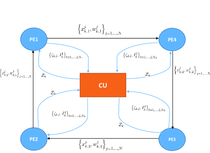
Figure 1: the structure of DCPFPHD

As the particle PHD filter is similar the particle filter,also involve three basic steps,we can use DRNA in particle PHD filter too.In this paper,we apply the DRNA scheme to particle-PHD filter.However,there is some differences in how calculate the weight and estimate target,the challenge is change the DRNA so we can use it in particle PHD filter(Fig 1).

3.1 General structure

The standard particle PHD filter requires all the particles be participated by a (single processor) in resampling step. In this paper,Assume we have K PEs and each can run a separate particle PHD with M particle.The total number of particles is N=MK. The distributed computation particle PHD filter can be outlines as follows,

Assume we have K groups and each can run a separate particle PHD with M particle.The total number of particles is N=MK. The distributed computation particle PHD filter can be outlines as follows,

DCPFPHD

Algorithm 1 Depiction on Each Group j

0:     $\left\{x_{k-1}^{(i,j)}\right\}_{i=1,...M},Z(k)$ Local PF-PHD filter

  for $i=1,\dots,M$ do

     $x_{k}^{(i,j)}\sim q(\cdot|x_{k-1}^{(i,j)},z_{k})$.

  end for

  for $i=M+1,\dots,M+J_{k}$ do

     $x_{k}^{(i,j)}\sim p(\cdot|z_{k})$.

  end for

  for $i=1,\dots,M+J_{K}$ do

     weight update $w_{k}^{(i,j)}=[\nu(x_{k}^{i})+\sum_{z\in Z_{k}}{\frac{\psi_{k,z}(x_{k}^{i})}{\kappa_{k}(z)+C_{k}(z)}}]w_{k|k-1}^{i}$

  end for Local Estimation

  estimate $N_{k}(j)$ and state(j) Resample

  resample the $M+J_{k}$ particles into $N_{k}(j)R_{k}$ particles and set $M=N_{k}(j)R_{k}$ Share Particles

  each group send t particle-weight couples to neighbors

In the following,we describe the algorithm steps in detail.

t=0:Generate M particles for each group.The number of all particles is N.All these particles are shared with same weights $\omega_{0}=1/M$

t=t+1

Step 1:Prediction At time t-1,we assume the particle set $x_{t-1}^{(k,m)}$.$w_{t-1}^{k,m}$ is available.For k-th group and m=1,…$L_{k}$,sample $\left\{x_{t}^{(k,m)}\right\}$ from $q_{k}$. For new-born particles we divide these particles to K group equal then join the groups.

Step 2:Update In update step,we can calculate the weights among groups.Let $Z_{k}$ denote the measurements set.For each group,for each $zinZ_{k}$,use the likelihood and compute $C_{t}^{k}$ and then update the weights.

Since we use the STPHD method to estimate state,the update step should make some change.zhao[13] has demonstrated that the $D_{k|k}$ can be calculated as

$$D_{k|k}(x|Z_{1:k})=\sum_{z\in Z_{k}}\Delta D_{k|k}(x|z)+\Delta D_{k|k}(x|\phi)$$ (10)

where $\Delta D_{k|k}(x|\phi)$ denotes the PHD of the measure undetected. For each observation $z_{p}\in Z_{k}$ ,$p=1,...,M_{k}$,For each group j,j=1,…,K

$$C_{k}(z_{k,p})=\sum_{i=1}^{M+J_{k}}{\psi_{k,z_{k,p}}\widetilde{w}_{k|k-1}^{(i,j)}\widetilde{x}_{k}^{(i,j)}}$$ (11)

$$G_{k}^{i,p,j}=\frac{\psi_{k,z}(\widetilde{x}_{k}^{i,j})}{\kappa(z_{k,p})+C_{k}(z_{k,p})}$$ (12)

then calculates the sub-weight of each particles for all observations $z_{k,p}$

$$\widetilde{\Delta w}_{k}^{i,p,j}=G_{k}^{i,p,j}\widetilde{w}_{k|k-1}^{i,j}$$ (13)

And the particle sub-weight for the target without measurements obtained is

$$\widetilde{\Delta w}_{k}^{i,p,0}=\nu(\widetilde{x}_{k}^{i,j})\widetilde{w}_{k|k-1}^{i,j}$$ (14)

Based on formula (10) ,the weights can compute through

$$\widetilde{w}_{k}^{i,j}=\sum_{p=1}^{M_{k}}\widetilde{\Delta w}_{k}^{i,p,j}+\widetilde{\Delta w}_{k}^{i,p,0}$$ (15)

Step 3:Local estimation

We use the STPHD method can extract the estimate targets and these targets’ sequence number. For each measurement $z_{k,p}$,$p=1,...,M_{k}$,compute the sum of $\widetilde{\Delta w}_{k}^{i,p,j}$ relevant to $z_{k,p}$ in group j.

$$\Delta W_{k}^{j,p}=\sum_{i=1}^{M+J_{k}}\widetilde{\Delta w}_{k}^{i,p,j}$$ (16)

Compute the sum of sub-weight $\Delta W_{k}^{j,0}$ corresponding to targets without observations:

$$\Delta W_{k}^{j,0}=\sum_{i=1}^{M+J_{k}}\widetilde{\Delta w}_{k}^{i,0,j}$$ (17)

Since the weight sum of all the particles equals to the target number,the local target number can be estimated by $LT_{k}^{j}=round(\sum_{i=1}^{i=M}\widetilde{w}_{k}^{i,j})$ where $round(\sum_{i=1}^{i=M}\widetilde{w}_{k}^{i,j})$ is the nearest integer to $\sum_{i=1}^{i=M}\widetilde{w}_{k}^{i,j}$

Find the $LT_{k}^{j}$ largest sum weight $\Delta W_{k}^{j,p}$ and the index set $I_{k}^{j}$ relevant to $\Delta W_{k}^{j,p}$ . The local estimated target state can be calculated by $\zeta_{k,l}=w_{k}^{i,l,j}\widetilde{x}_{k}^{i,j}$ where $l$ in index set ,

$$w_{k}^{i,l,j}=\frac{\widetilde{\Delta w}_{k}^{i,l,j}}{\sum_{i=1}^{M+J_{k}}\widetilde{\Delta w}_{k}^{i,p,j}}$$ (18)

The groups can send data to the CU. When the group get a local estimate like $\zeta_{k,l}$ and transmit the pair $\left\{\zeta_{k,l},I_{k}^{j}\right\}$ to the CU.Then the CU can combine the local estimate state which depends on the measurement index from the group to construct a global estimate.

Step 4:Global Estimation

As the CU receives all the local information $\left\{\zeta_{k,l},I_{k}^{j}\right\}$.Depend on the rule "at most one measurement per target"[11].If the local estimate state’s label $\left\{I_{j}^{i}\right\}$ is same that from different groups,then we use their mean value as the global estimate state. And the local estimate state may be from clutter,so we consider only the local estimate states’ number which have same label greater than half of groups’ number as valid estimate states.

Step 5:Resampling

The resampling can be carry out locally at the N groups.Normalize the weights of the particles with the sum of weights in the group.

Step 6:Local exchange

The particles in the n-th group will degenerate when its aggregated weight becomes negligible relative to the aggregated weights of the other groups.Then the n-th group hardly contribute to the approximation of the posterior probability distribution.In order to keep the groups are valid,neighboring groups can exchange a portion of particles and weights.We select the L particles from k-th group($L<M/2$) to replace the L particles from k-1 group in random.

for k=1,…K-1,i=1….,L do:

$\left\{{x_{t}^{i,k}}\right\}\rightarrow\left\{{x_{t}^{i,{k+1}}}\right\}$

for k=K ,i=1….,L do:

$\left\{{x_{t}^{i,K}}\right\}\rightarrow\left\{{x_{t}^{i,1}}\right\}$

The processors are connected using an interconnection network.There are many type of network can be used,we select a ring configuration in this paper.For a ring network ,the nth PE,n=1,…,N-1,can send data to the (n+1)th PE.The Nth PE transmits data to PE number 1.

The PEs can also send data to the CU. When the PE get a local estimate like $ddd$ and transmit the pair to the CU.Then the CU can combine the local estimate state which depends on the measurement index from the PE to construct a global estimate.

3.2 Analysis of Time Delay and Computational Complexity

In the traditional particle PHD filter,all the particles have to be involved by serial. In our methods,since particles are divided into K groups and the group can run a particle PHD filter independently,thus it only utilise $1/K$ time than before in theory.

4 SIMULATION RESULTS AND EXPERIMENTAL STUDY

To evaluate the proposed distributed particle PHD filter,we consider a two-dimensional scenario with the target can disappear and appear at anytime.Each target moves according to the following model $x_{k+1}=\left[\begin{array}[]{cccc}1&T&0&0\\ 0&1&0&0\\ 0&0&1&T\\ 0&0&0&1\\ \end{array}\right]x_{k}+\left[\begin{array}[]{cc}T^{2}/2&0\\ 1&0\\ 0&T^{2}/2\\ 0&1\\ \end{array}\right]w_{k}$ where $x_{k}=[x_{k},\dot{x}_{k},y_{k},\dot{y}_{k}]$ is target state vector at time kT(k is the time index and T=1 is the sampling period).[$x_{k}$,$y_{k}$] is the position,while $[\dot{x}_{k},\dot{y}_{k}]$ is the velocity.$w_{k}=[w_{k}^{x},w_{k}^{y}]$ is the vector of independent zero-mean Gaussian white noise with standard deviations of $\left[\begin{array}[]{cc}0.025&0\\ 0&4\\ \end{array}\right]$ There is just a signal sensor in the scenario and the target-originated measurement are given by
$z_{k}$=g($x_{k}$)+$v_{k}$=$[R,\theta]^{T}$
$=\left[\begin{array}[]{c}R=\sqrt{(x-s_{x})^{2}+(y-s_{y})^{2}}\\ \theta=\arctan{(y-s_{y})/(x-s_{x})}\\ \end{array}\right]+\left[\begin{array}[]{c}v_{k}^{R}\\ v_{k}^{\theta}\\ \end{array}\right]$

The measurement variance $v_{k}^{R}=5m,v_{k}^{\theta}=0.05rad$. Clutter is modeled as a Poisson RFS $\kappa_{k}$ with intensity $\kappa_{k}(z)=\lambda_{k}V_{u}(z)$ The Target can disappear or appear in the scene at any time.The probability of target survival is $e_{k|k-1}=0.9$ and is detected with probability $P_{D,k}=1$ . Assume the target birth according to the Poisson distribution with the intensity $N(\cdot,\overline{x},Q)$ where $N(\cdot,\overline{x},Q)$ denotes a normal density with mean $\overline{x}$ and covariance Q.

$\overline{x}=\left(\begin{array}[]{c}0\\ 3\\ 0\\ -3\\ \end{array}\right)$, $Q=\left(\begin{array}[]{cccc}10&0&0&0\\ 0&1&0&0\\ 0&0&10&0\\ 0&0&0&1\\ \end{array}\right)$

The surveillance region is $[-\pi/2,\pi/2]\times[0,200]$ rad.m. Assign 200 particles to an exist or new born target in each group.The number of group is 4.

4.1 Simulation Results

We run 100 independent simulations of the BOT model given by….The overall number of particles was N = 2000 and ,for the DCPFPHD,we divide them into N=4 processors with M=500 particles each. The true trajectories of five tracks over 50 scans are plotted in Fig 2(a).Fig 2(a) also shows the positions of the estimated targets over 50 time steps. The individual x and y coordinates of the tracks and estimated targets for each time step are shown in Fig 2(b) and Fig 2(c),respectively.It can be seen that estimated position based on the traditional particle PHD filter which the number of particles is equals the DPHD filter’s particles and the DCPPHD are similar and they are all close to the true tracks.

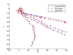
(a)

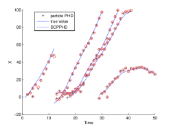
(b)

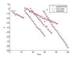
(c)

Figure 2: Target trajectories estimated by the DCPPHD filter and the particle PHD filter.(a)Estimated trajectories and true trajectories.(b)Estimated trajectories and true trajectories in x-axis direction.(c)Estimated trajectories and true trajectories in y-axis direction

Another vital factor for the performance of the method is the estimated number of targets.The number of true targets and estimated target by our method ,standard particle PHD filter with same particles and only $1/k$ particles at each scan are given in Fig 3.It is observed that,under the same simulation conditions and same particles ,the particle PHD filter and DCPPHD filter achieve

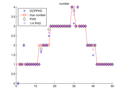
Figure 3: Estimated number of targets and the true number of targets

It was proposed in [9] to use the Optimal Sub-Pattern Assignment(OSPA) as a multi-target miss-distance metric,and the parameters in it are set as p = 1 and c = 100 inour evaluation. Fig 4 shows the OSPA distance of the DCPPHD filter and particle PHD filter.

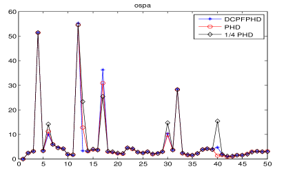
Figure 4: the ospa

The total number of particles for these methods is given in Tabel1.Implemented on a Dell computer using MATLAB,this approximate times used by these approachs are also given in Tabel1.And the Table1 shows the mean of OSPA as well.

Table 1: 12345

method	particle number	times	mean of OSPA	std of OSPA	r
PHD	1 in 1,000	17.6540	3.0577	0.0548	0
DCPPHD	1 in 5	8.6331	3.0732	0.0830	0
partPHD	1 in 40,000	4.0935	3.1993	0.2590	0
PHD	1 in 1,000	72.2214	6.4432	19.0788	10
DCPPHD	1 in 5	27.1516	6.2220	5.4630	10
partPHD	1 in 40,000	17.2492	7.4752	54.4956	10
PHD	1 in 1,000	117.1504	8.0049	8.2928	20
DCPPHD	1 in 5	39.4615	8.0884	22.6434	20
partPHD	1 in 40,000	29.2382	9.7143	136.3478	20

set simulation results 1.the target position
2.the ospa
3.the time
4.the number

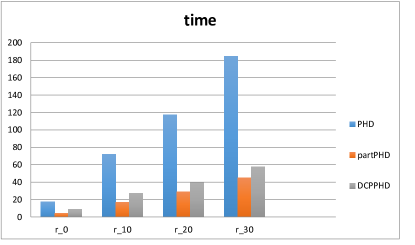
Figure 5: the time

and analyse the result.

5 CONCLUSION

In this paper,we proposed a DRNA particle PHD filter that want to improve the particle PHD filter runtime.The DRNA-PHD filter can speed up the particle PHD filter in theory.However, the feasibility of the proposed method needs to be tested in real applications.It note that divide the more groups will lead to the decrease of performance.
future work may consider other particle exchange method and simplify the update step as we found the weight update also cause a lot of compute time.The update step and resamping will be the bottleneck for the development of higher speed of particle PHD filter.And we will test the method into the GPU as well.

References

- [1] S. S. B. N. Vo and A. Doucet. Sequential monte carlo methods for multi-target filtering with random finite sets. IEEE Transactions on Aerospace and Electronic Systems., 41(4):1224–1245, 2008.
- [2] B.-N. V. B.-T. Vo and A. Cantoni. Analytic implementations of the cardinalized probability hypothesis density filter. IEEE Transactions on Signal Processing,., 55(7):3553–3567, July 2007.
- [3] B.-N. V. B.-T. Vo and A. Cantoni. Sthe cardinality balanced multitarget multi-bernoulli filter and its implementations. IEEE Transactions on Signal Processing., 57(2):409–423, February 2009.
- [4] S. S. Blackman. Multiple hypothesis tracking for multiple target tracking. Aerospace and Electronic Systems Magazine, IEEE, 19(1):5–18, 2004.
- [5] M. Bolic, P. M. Djuric, and S. Hong. Resampling algorithms and architectures for distributed particle filters. Signal Processing, IEEE Transactions on, 53(7):2442–2450, 2005.
- [6] T. E. Fortmann, Y. Bar-Shalom, and M. Scheffe. Sonar tracking of multiple targets using joint probabilistic data association. Oceanic Engineering, IEEE Journal of, 8(3):173–184, 1983.
- [7] R. Mahler. Multitarget bayes filtering via first-order multitarget moments. IEEE Trans. Aerosp. Electron. Syst, 39(4):1152–1178, October 2003.
- [8] R. Mahler. Phd filters of higher order in target number. IEEE Trans. Aerosp. Electron. Syst., 43(4):1523–1543, October 2007.
- [9] D. Schuhmacher, B.-T. Vo, and B.-N. Vo. A consistent metric for performance evaluation of multi-object filters. Signal Processing, IEEE Transactions on., 56(8):3447–3457, April 2005.
- [10] R. A. Singer and J. J. Stein. An optimal tracking filter for processing sensor data of imprecisely determined origin in surveillance systems. In Decision and Control, 1971 IEEE Conference on, volume 10, pages 171–175. IEEE, 1971.
- [11] R. Streit. The probability generating functional for finite point processes, and its application to the comparison of phd and intensity filters. J. of Advances in Information Fusion, to appear, 2013.
- [12] B.-N. Vo and W.-K. Ma. The gaussian mixture probability hypothesis density filter. IEEE Trans. Signal Process, 54(11):4091–4104, November 2006.
- [13] L. Zhao, P. Ma, X. Su, and H. Zhang. A new multi-target state estimation algorithm for phd particle filter. In Information Fusion (FUSION), 2010 13th Conference on, pages 1–8. IEEE, 2010.