On Isogeometric Subdivision Methods for PDEs on Surfaces

Abstract: Subdivision surfaces are proven to be a powerful tool in geometric modeling and computer graphics, due to the great flexibility they offer in capturing irregular topologies. This paper discusses the robust and efficient implementation of an isogeometric discretization approach to partial differential equations on surfaces using subdivision methodology. Elliptic equations with the Laplace-Beltrami and the surface bi-Laplacian operator as well as the associated eigenvalue problems are considered. Thereby, efficiency relies on the proper choice of a numerical quadrature scheme which preserves the expected higher order consistency. A particular emphasis is on the robustness of the approach in the vicinity of extraordinary vertices. In this paper, the focus is on Loop’s subdivision scheme on triangular meshes. Based on a series of numerical experiments, different quadrature schemes are compared and a mid-edge quadrature, which is easy-to-implement via lookup tables, turns out to be a preferable choice due to its robustness and efficiency.

Keywords: subdivision methods, isogeometric analysis, PDEs on surfaces, numerical quadrature.

1 Introduction

During the last years, isogeometric analysis (IgA) [1, 2] emerged as a means of unification of the previously disjoint technologies of geometric design and numerical simulation. The former technology is classically based on parametric surface representations, while the latter discipline relies on finite element approximations. The advantages of the isogeometric paradigm include the elimination of both the geometry approximation error and the computation cost of changing the representation between design and analysis. A particular challenge is the problem of efficient numerical integration. Indeed, the higher degree and multi-element support of the basis functions seriously affect the cost of robust numerical integration. Consequently, numerical quadrature in IgA is an active area of research [3, 4, 5, 6, 7].

Subdivision schemes are widespread in geometry processing and computer graphics. For a comprehensive introduction to subdivision methods in general we refer the reader to [8] and [9]. With respect to the use of subdivision methods in animation see [10, 11]. Nowadays, subdivision finite elements are also extensively used in engineering [12, 13, 14, 15, 16, 17]. This way, the subdivision methodology changed the modeling paradigms in computer-aided design (CAD) systems over the last years tremendously, e.g. the Freestyle module of PTC Creo®, the PowerSurfacing add-on for SolidWorks® or NX RealizeShape of Siemens PLM®. For the integration of subdivision methods in CAD systems, we refer to [18, 19] and the references therein. With this development, powerful computer-aided engineering (CAE) codes have to be implemented for subdivision surfaces. Today NURBS and subdivision surfaces co-exist in hybrid systems.

Among the most popular subdivision schemes are the Catmull-Clark [20] and Doo-Sabin [21] schemes on quadrilateral meshes, and Loop’s scheme on triangular meshes [22]. The Loop subdivision basis functions have been extensively studied, most interestingly regarding their smoothness [23, 24], (local) linear independence [25, 26], approximation power [27], and the robust evaluation around so called extraordinary vertices [28].

Computing PDEs on surfaces is an indispensable tool either to approximate physical processes on the surfaces [29] or to process textures on the surface or the surface itself [30, 31, 32]. Recently, surface PDEs have been considered in the field of IgA, and both numerical and theoretical advancements are reported [33, 34, 35].

The use of Loop subdivision surfaces as a finite element discretization technique is discussed in [12] and isogeometric discretizations based on the Catmull-Clark scheme in [36, 37], whereas [38] investigates the use of the Doo-Sabin scheme in the finite element context. An isogeometric finite element analysis based on Catmull-Clark subdivision solids can be found in [39].

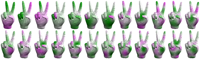
Figure 1: As an application we show here the first 24 eigenfunctions of the Laplace-Beltrami operator computed on a complex surface using the isogeometric subdivision approach. See Figure 8 for the coarse control mesh.

In this paper, we focus on the Loop subdivision scheme [40] on triangular meshes. Loop subdivision is known to describe $C^{2}$ limit surfaces $\mathcal{M}$ except at finitely many points (called extraordinary vertices) where they are only $C^{1}\cap H^{2}$ [23, 24]. This allows us to use them in a conforming finite element approach not only for second-order but also for fourth-order elliptic PDEs. As model problem we consider the Laplace-Beltrami equation

$$-\Delta_{\mathcal{M}}u =f\text{ on }\mathcal{M}\,,$$ (1)

the surface bi-Laplacian equation

$$(-\Delta_{\mathcal{M}})^{2}u =f\text{ on }\mathcal{M}\,$$ (2)

as well as the eigenvalue problem

$$-\Delta_{\mathcal{M}}u=\lambda u\text{ on }\mathcal{M}\,.$$ (3)

Let us remark that on closed, smooth surfaces the kernel of the Laplace-Beltrami and the surface bi-Laplacian operators are the constant functions.

The crucial step in the implementation of a subdivision finite element method is the choice of numerical quadrature. The computational cost, consistency, robustness and the observed order of convergence are important parameters to evaluate the appropriateness of each numerical integration technique. We aim at a detailed experimental study of the convergence behavior for different quadrature rules. We examine Gaussian quadrature, barycenter quadrature, mid-edge quadrature and discuss adaptive strategies around extraordinary vertices. Furthermore, we provide a look-up table for the mid-edge quadrature that facilitates the implementation and results in a fairly robust simulation tool and a very efficient assembly of finite element matrices. This allows for a straightforward extension of existing subdivision modeling codes to simulations with subdivision surfaces for applications, see Figure 1.

Organisation of the paper. In Section 2, we fix some notation and define subdivision functions and subdivision surfaces. The isogeometric subdivision method to solve elliptic partial differential equations on surfaces is described in Section 3, where we derive the required finite element mass and stiffness matrices. Section 4 investigates the different numerical quadrature rules and comments on the efficient implementation. In Section 5, we report on the observed convergence behavior for a set of selected test cases. Finally, we draw conclusions in Section 6.

2 Subdivision Functions and Surfaces

To discretize geometric differential operators and to solve geometric partial differential equations on closed subdivision surfaces we consider isogeometric function spaces defined via Loop’s subdivision.

The domain of a Loop subdivision surface is a topological manifold obtained by gluing together copies of a standard triangle. More precisely, we consider the unit triangle $\triangle\subset\mathbb{R}^{2}$ with vertices $(0,0)$, $(1,0)$ and $(0,1)$, which is considered as a closed subset of $\mathbb{R}^{2}$, and a finite cell index set $\mathcal{I}_{c}\subset\mathbb{\mathbb{Z}}$. The Cartesian product $\triangle\times\mathcal{I}_{c}$ defines the pre-manifold which consists of the cells $\triangle\times\{i\}$, $i\in\mathcal{I}_{c}$. The manifold is constructed by identifying points on the boundaries of the cells, as described below.

In addition to the cell index set, we consider an edge index set $\mathcal{I}_{e}\subset\mathbb{\mathcal{I}}_{c}\times\mathcal{I}_{c}$, which is assumed to be symmetric

$$(i,j)\in\mathcal{I}_{e}\Rightarrow(j,i)\in\mathcal{I}_{e}$$

and irreflexive

$$\forall i\in\mathbb{Z}:\;(i,i)\not\in\mathcal{I}_{e}.$$

Each edge is described by a symmetric pair of edge indices $((i,j)$, $(j,i))\in\mathcal{I}_{e}\times\mathcal{I}_{e}$. Moreover, each cell contributes to exactly three edges,

$$\forall i\in\mathcal{I}_{c}:|\{j:(i,j)\in\mathcal{I}_{e}\}|=3.$$

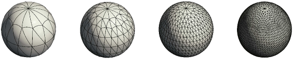
Figure 2: The spherical subdivision limit surface Spherical-5-12 with successively refined control meshes. The control meshes are plotted on the limit surface, i.e., they visualize the curved IgA-elements on the surface. Furthermore, the control meshes possess two vertices of valence $12$ and $24$ vertices of valence $5$ on every refinement level. Since two EVs share an edge in the coarsest control mesh, this mesh cannot be used for simulation.

Each edge index $(i,j)$ is associated with a displacement $\delta^{i}_{j}$, which is one of the 18 isometries ($3\cdot 3\cdot 2$) that map the unit triangle to one of its three neighbor triangles obtained by reflection and index permutation. These displacements in particular identify the common edges of neighboring triangles and its orientation with respect to the two triangles. They need to satisfy the following two conditions. Firstly, the identification of the common edge and its orientation has to be consistent for each edge, thus

$$\forall(i,j)\in\mathcal{I}_{e}:\;\delta^{i}_{j}=(\delta^{j}_{i})^{-1}.$$

Secondly, each edges of a triangle is identified with exactly one edge of another triangle,

$$\forall(i,j)\in\mathcal{I}_{e}:\;\forall(i,k)\in\mathcal{I}_{e}:\;\delta^{i}_{j}(\Delta)\cap\Delta=\delta^{i}_{k}(\Delta)\cap\Delta\Rightarrow j=k.$$

Two points of the pre-manifold are identified, denoted by $(\xi,i)\sim(\eta,j)$, if $(i,j)$ is an edge index and the displacement $\delta^{i}_{j}$ transforms $\eta$ into $\xi$. This implies that $\xi$ and $\eta$ are located on the boundary of the standard triangle. We denote with $\hat{\sim}$ the reflexive and transitive closure of this relation. This closure leads to the obvious identification of common vertices. The topological manifold $(\triangle\times\mathcal{I}_{c})/\hat{\sim}$ is the domain manifold of the Loop subdivision surface.

There, the indexed standard triangles define an initial triangulation (of level $0$) of the domain manifold. Now, Loop’s subdivision scheme iteratively creates triangulations of level $\ell>0$ containing $4^{\ell}|\mathcal{I}_{c}|$ triangles. They are obtained by creating new vertices at the edge midpoints and splitting each triangle of level $\ell-1$ into four smaller ones. The valence of the vertices in these triangulations are always $6$, except for those vertices of the coarsest level that possess a different valence. The latter ones are called extraordinary vertices (EVs). For an example of a Loop subdivision surface with extraordinary vertices and different resolutions of the control mesh see Figure 2.

Next, we consider the spaces $L^{\ell}$ of piecewise linear functions on the triangulation of level $\ell$. Each function is uniquely described by its nodal values, i.e., by its values at the vertices of the triangulation. The Loop subdivision operators $R^{\ell}:L^{\ell-1}\to L^{\ell}$ are linear operators that transform a piecewise linear function $f^{\ell-1}$ of level $\ell-1$ into a function of level $\ell$. The nodal values of the latter (refined) function are computed as weighted averages of nodal values of the coarser function at neighboring vertices. Values at newly created vertices (at edge midpoints) depend on the four nodal values of the coarser function on the two triangles intersecting at the edge, while values at existing vertices are computed from the values at the (valence+1)-many vertices in the one-ring neighborhood. The weights are determined by simple formulas [41].

The space of Loop subdivision splines [40] consists of the limit functions generated by the subdivision operators,

$$\{\lim_{L\to\infty}R^{L}R^{L-1}\cdots R^{1}f:f\in L^{0}\}.$$

These limit functions are known to be bivariate quartic polynomials on all triangles of the triangulation of level $\ell$ that do not possess any EVs. They are $C^{2}$-smooth everywhere, except at the EVs. If one uses a special parameterization around EVs, which is given by the charateristic map [23, 24] then the limit functions are $C^{1}$-smooth at EVs.

Let $\mathcal{I}_{v}$ be the vertex index set of the coarsest triangulation. Each vertex $i\in\mathcal{I}_{v}$ has an associated piecewise linear hat function $\Lambda_{i}\in L^{0}$ which takes the nodal value 1 at the associated vertex and 0 else. The limit functions

$$\Phi_{i}=\lim_{L\to\infty}R^{L}R^{L-1}\cdots R^{1}\Lambda_{i},$$

which will be denoted as the Loop basis functions, span the space of Loop subdivision splines. The support of the Loop basis function is the two-ring neighborhood of the vertex $i$ in the coarsest triangulation. If the support does not contain EVs in its interior, then it consists of $24$ triangles of the coarsest level and the Loop basis function is the $C^{2}$-smooth quartic box spline on the type-1 triangulation. Otherwise, the Loop basis function is still a piecewise polynomial function but possesses an infinite number of polynomial segments. These are associated with triangles obtained by successive refinement in the vicinity of the EV and not containing the EV itself [8].

Now we have everything at hand to introduce a Loop subdivision surface

$$X:\;\triangle\times\mathcal{I}_{c}/\hat{\sim}\to\mathbb{R}^{3}:\;X(\xi,k)=\sum\limits_{i\in\mathcal{I}_{v}}C_{i}\varPhi_{i}(\xi,k)\,,$$

which is obtained by assigning control points $C_{i}\in\mathbb{R}^{3}$ to the Loop basis functions with $\xi=(\xi_{1},\xi_{2})\in\triangle$. This surface is $C^{2}$ smooth everywhere, except at EVs (in the same sense as described before) [23, 24]. Hence, it can be shown that the surface possesses a well-defined tangent plane at EVs, provided that the control points are not in a singular configuration. We denote the surface (as an embedded manifold) by $\mathcal{M}=\mathcal{M}[X]$. In the context of isogeometric analysis, the parameterization $X$ of the domain is referred to as the geometry mapping. The basis functions $\varphi_{i}$ of the associated isogeometric function space are the push-forwards of the subdivision basis functions

$$\varphi_{i}(x)=\varPhi_{i}\circ X^{-1}(x),$$

where $x=X(\xi,k)$, i.e., the basis functions are defined by the discretization $X$. We define the discretization space as

$$V_{h}=\Big{\{}u_{h}\in\operatorname{span}\limits_{i\in\mathcal{I}_{v}}\{\varphi_{i}\}\Big{\}}.$$

Here, $h$ indicates the grid size of the control mesh, i.e., $h=\max_{(i,j)\in\mathcal{I}_{e}}|C_{i}-C_{j}|$. For each cell, we denote by $J(\xi,k)=\begin{pmatrix}X_{,1}&X_{,2}\end{pmatrix}$ the Jacobian of $X$ and by $G=J^{T}J$ its first fundamental form, where $X_{,1}$ and $X_{,2}$ denote the tangent vectors with $X_{,l}=\frac{\partial}{\partial\xi_{l}}X(\xi,k)$. Furthermore, for a function $u:\mathcal{M}\to\mathbb{R}$

$$\nabla_{\mathcal{M}}u(x)=\left(JG^{-T}\nabla_{\xi}(u\circ X)\right)(\xi,k)$$

is the (embedded) tangential gradient or surface gradient and

$$\Delta_{\mathcal{M}}u(x)=\frac{1}{\sqrt{\det G}}\operatorname{div}_{\xi}\left(\sqrt{\det G}G^{-1}\nabla_{\xi}(u\circ X)\right)(\xi,k)$$

the Laplace-Beltrami operator, where $x=X(\xi,k)$.

3 Isogeometric Subdivision Method to solve PDEs

Similar to the classical finite element method, the isogeometric subdivision approach transforms the strong formulation of a partial differential equation (e.g. (1) – (3)) into a corresponding weak formulation on a suitable subspace $V^{0}$ of some Sobolev space and approximates the solution of the weak problem in the finite-dimensional sub-spaces $V^{0}_{h}\subset V^{0}$. We consider

$$V^{0}=H^{1}(\mathcal{M})\cap\{\int_{\mathcal{M}}v\,\mathrm{d}a=0\}$$

for problem (1) and

$$V^{0}=H^{2}(\mathcal{M})\cap\{\int_{\mathcal{M}}v\,\mathrm{d}a=0\}$$

for problem (2). Following the general isogeometric paradigm we use

$$V^{0}_{h}=V_{h}\cap\{\int_{\mathcal{M}}v_{h}\,\mathrm{d}a=0\}$$

as the discrete ansatz space on the subdivision surface $\mathcal{M}$, e.g., see Figure 2.

Let $a:V^{0}\times V^{0}\to\mathbb{R}$ denote a symmetric, coercive and bounded bilinear form on $V^{0}$ and $\ell_{f}:V^{0}\to\mathbb{R}$ a linear form for a given function $f\in L^{2}(\mathcal{M})$. Then there exists a unique solution $u\in V^{0}$ of the variational problem

$$a(u,v)=\ell_{f}(v),\quad\forall\leavevmode\nobreak\ v\in V^{0},$$ (4)

where $\ell_{f}(v)=\int_{\mathcal{M}}fv\,\mathrm{d}a$ ([42, 43, 44, 45]). For our model problems, we use

$$a(u,v)=\int_{\mathcal{M}}\nabla_{\mathcal{M}}u\cdot\nabla_{\mathcal{M}}v\,\mathrm{d}a$$

and

$$a(u,v)=\int_{\mathcal{M}}\Delta_{\mathcal{M}}u\,\Delta_{\mathcal{M}}v\,\mathrm{d}a$$

for the Laplace-Beltrami (1) and the Bi-Laplacian problem (2), respectively. The associated Galerkin approximation asks for the unique solution $u_{h}\in V^{0}_{h}$ of the discrete variational problem

$$a(u_{h},v_{h})=\ell_{f}(v_{h}),\quad\forall\leavevmode\nobreak\ v_{h}\in V^{0}_{h}\,.$$ (5)

Due to the known $H^{2}$-regularity of the Loop subdivision splines this Galerkin approximation is conforming, i.e., $V^{0}_{h}\subset V^{0}$. Using the basis expansion $u_{h}=\sum\limits_{i\in\mathcal{I}_{v}}u_{i}\varphi_{i}$ for $u_{h}$ with coefficients $u_{i}\in\mathbb{R}$ one obtains the linear system

$$\mathbf{S}\mathbf{U}=\mathrm{B},$$ (6)

where $\mathbf{U}=(u_{i})_{i\in\mathcal{I}_{v}}\in\mathbb{R}^{\mid\mathcal{I}_{v}\mid}$ denotes the coefficient vector, $\mathbf{S}_{ij}=a(\varphi_{i},\varphi_{j})\in\mathbb{R}^{\mid\mathcal{I}_{v}\mid\times\mid\mathcal{I}_{v}\mid}$ the stiffness matrix, and $\mathrm{B}_{j}=\int_{\mathcal{M}}f\varphi_{j}\,\mathrm{d}a\in\mathbb{R}^{\mid\mathcal{I}_{v}\mid}$ the right-hand side. The stiffness matrix for the Laplace-Beltrami problem (1) is given by

$$\mathbf{S}_{ij}^{\Delta}=\int_{\mathcal{M}}\nabla_{\mathcal{M}}\varphi_{i}\cdot\nabla_{\mathcal{M}}\varphi_{j}\,\mathrm{d}a=\sum\limits_{k\in\mathcal{I}_{c}}\int_{\triangle}\nabla_{\xi}\varPhi_{i}G^{-T}\nabla_{\xi}\varPhi_{j}\sqrt{\det G}\,\mathrm{d}\xi$$ (7)

and for the surface bi-Laplacian problem (2) we obtain

$$\mathbf{S}_{ij}^{\Delta^{\!2}} =\sum\limits_{k\in\mathcal{I}_{c}}\int_{\triangle}\operatorname{div}_{\xi}\left(\sqrt{\det G}G^{-1}\nabla_{\xi}\varPhi_{i}\right)\operatorname{div}_{\xi}\left(\sqrt{\det G}G^{-1}\nabla_{\xi}\varPhi_{j}\right)\frac{1}{\sqrt{\det G}}\,\mathrm{d}\xi\,.$$ (8)

The variational formulation of the eigenvalue problem (3) consists in finding a solution $(u,\lambda)\in V^{0}\times\mathbb{R}$ such that

$$a(u,v)=\lambda\cdot m(u,v),\quad\leavevmode\nobreak\ \forall\leavevmode\nobreak\ v\in V^{0},$$

where $m(u,v)=\int_{\mathcal{M}}u\,v\,\mathrm{d}a$ denotes the $L^{2}$-product on $\mathcal{M}$. Furthermore, we denote by $\mathbf{M}$ the mass matrix with

$$\mathbf{M}_{ij}=m(\varphi_{i},\varphi_{j})=\sum\limits_{k\in\mathcal{I}_{c}}\int_{\triangle}\varPhi_{i}\varPhi_{j}\sqrt{\det G}\,\mathrm{d}\xi.$$ (9)

We obtain the discrete eigenvalue problem $\mathbf{S}\mathbf{U}=\lambda_{h}\mathbf{M}\mathbf{U}$ which can be solved by inverse vector iteration with projection [46].

4 Numerical Quadrature

In this section, we recap the evaluation-based assembly of the previously defined discrete variational formulations. We review standard Gaussian and barycentric quadrature assembly, discuss the special treatment at extraordinary vertices and finally introduce an edge-centered assembly strategy which is based on simple fixed, geometry-independent lookup tables and already very good consistency in our experiments (see Section 5). As discussed above, the isogeometric subdivision approach is based on higher order spline discretizations. The integrands of the corresponding IgA-matrices ((7) – (9)) are in general nonlinear and even on planar facets of the subdivision surface (with constant metric $G$) high-degree polynomials. Indeed, apart from EVs the limit functions $\Phi_{i}$ are quartic polynomials and thus for the mass matrix the integrand is a polynomial of degree $8$ and for the stiffness matrix (7) of degree $6$ and for (8) of degree $4$.

In the variational formulation, the integration is always pulled-back to the reference triangle, i.e.,

$$\int_{\mathcal{M}}f\,\mathrm{d}a=\sum\limits_{k\in\mathcal{I}_{c}}\int_{\triangle}f\circ X\,\sqrt{\det G}(\xi,k)\,\mathrm{d}\xi\,.$$

Thus numerical quadrature is applied to these pulled-back integrands. For a general function $g$ using the evaluation-based quadrature

$$\int_{\triangle}g(\xi)\mathrm{d}\xi\approx\sum\limits_{q=1}^{K}w_{q}g(\xi^{q})\,,$$

with quadrature points $\xi_{q}$ on the reference triangle $\triangle$ and weights $w_{q}$, we replace the stiffness matrices, the mass matrix, and the right-hand side by the following quadrature based counterparts

$$\mathbf{\tilde{S}}_{ij}^{\Delta} = \sum\limits_{k\in\mathcal{I}_{c}}\sum\limits_{q=1}^{K}w_{q}\left(\nabla_{\xi}\varPhi_{i}^{T}G^{-T}\nabla_{\xi}\varPhi_{j}\sqrt{\det G}\right)(\xi^{q},k)$$ (10)

and

$$\mathbf{\tilde{S}}_{ij}^{\Delta^{\!2}} = \sum\limits_{k\in\mathcal{I}_{c}}\sum\limits_{q=1}^{K}w_{q}\left(\operatorname{div}_{\xi}\left(\sqrt{\det G}G^{-1}\nabla_{\xi}\varPhi_{i}\right)\operatorname{div}_{\xi}\left(\sqrt{\det G}G^{-1}\nabla_{\xi}\varPhi_{j}\right)\frac{1}{\sqrt{\det G}}\right)(\xi^{q},k)$$ (11)

as well as

$$\mathbf{\tilde{M}}_{ij} = \sum\limits_{k\in\mathcal{I}_{c}}\sum\limits_{q=1}^{K}w_{q}\left(\varPhi_{i}\cdot\varPhi_{j}\,\sqrt{\det G}\right)(\xi^{q},k)$$ (12)

and

$$\mathbf{\tilde{B}}_{j} = \sum\limits_{k\in\mathcal{I}_{c}}\sum\limits_{q=1}^{K}w_{q}\left((f\circ X)\cdot\varPhi_{j}\,\sqrt{\det G}\right)(\xi^{q},k).$$ (13)

Now, instead of solving (6), we solve the system $\tilde{\mathbf{S}}\cdot\mathbf{U}=\mathrm{\tilde{B}}$. The associated, modified variational problem reads as follows: Find $\tilde{u}_{h}\in V^{0}_{h}$ such that

$$\tilde{a}(\tilde{u}_{h},v_{h})=\tilde{\ell}_{f}(v_{h}),\quad\forall\leavevmode\nobreak\ v_{h}\in V_{h}^{0},$$ (14)

where $\tilde{a}(\varphi_{i},\varphi_{j})=\mathbf{\tilde{S}}_{ij}$ and $\tilde{\ell}_{f}(\varphi_{j})=\mathbf{\tilde{B}}_{j}$. If $\tilde{a}(.,.)$ is uniformly $V_{h}$-elliptic ($\mathbf{\tilde{S}}$ positive definite) existence and uniqueness of the discrete solution $\tilde{u}_{h}$ is ensured (cf. [42], for instance).

Gaussian Quadrature.

For second-order elliptic problems, standard error estimates for finite element schemes with Gaussian quadrature [44, Chapter 4.1] imply that the expected order of convergence, in case of exact integration, is preserved if the quadrature scheme is exact for polynomials of degree $p=6$. Transferring this to fourth-order problems we request exactness for polynomials of degree $p=4$. This suggests to choose a Gaussian quadrature rule GA($p$) which guarantees this required exactness. For the Laplace-Beltrami equation (1) $K=12$ and for the surface bi-Laplacian equation (2) $K=6$ quadrature points have to be taking into account on the reference triangle $\triangle$ (for symmetric Gaussian quadrature points on triangles see [47]).

Adaptive Gaussian Quadrature.

Special care is required close to EVs [8], because the basis functions $\Phi_{i}$ are no longer polynomials and the second order derivatives are singular at the EV. Furthermore, the natural parametrization [28] produces only $C^{0}$-surfaces at EVs instead of $C^{1}$-parametrizations. To obtain a $C^{1}$-parametrization a suitable embedding has to be considered, e.g., using the characteristic map [19, 8]. For the implementation, the evaluation algorithm of [28] can still be used, thanks to the integral transformation rule.

Because of the structure of the subdivision scheme, the subdivision surface and correspondingly the basis functions $\Phi_{i}$ are spline functions on local triangular mesh rings around each EV [8]. Thus, this subdivision ring structure can be used via an adaptive refinement strategy of the reference triangle $\triangle$ around the EV and an application of Gaussian quadrature on the resulting adaptive reference mesh to overcome the limitation of the standard Gaussian quadrature on the reference triangle. More explicitly, for triangles with an EV we decompose the associated reference triangle $\triangle$ into finer triangles $\triangle_{i}^{l}$ ($l=1,\ldots,L$) of level $L$ (see Figure 3, left), perform the corresponding Gaussian quadrature GA($p$) on all finer triangles $\triangle_{i}^{l}$ and call this adaptive Gaussian quadrature AG($p,L$). Hence, the number of quadrature points $K$ on these adaptively refined triangles depends on $L$: $K=(3\cdot L+1)\cdot 12$ for the Laplace-Beltrami equation (1) and $K=(3\cdot L+1)\cdot 6$ for the surface bi-Laplacian equation (2). It is worth mentioning that this expensive scheme has to be applied only for a small number of triangles around the finitely many EVs. Finally, let us remark that standard Romberg extrapolation does not lead to any improvement of the adaptive Gaussian quadrature due to the lack of smoothness of the integrands in the mesh size parameter and an adaption of the Romberg method for singular problems failed because the type of singularity is not explicitly known.

Barycenter Quadrature.

Implementation of the adaptive Gaussian quadrature is a tedious issue. In particular, in graphics where the achievable maximal order of consistency is not needed, already the computing cost of the usual Gaussian quadrature is significant. Therefore, reduced quadrature assembly is a common practice when implementing modeling or simulation tools based on NURBS as well as for subdivision surfaces (e.g. [4, 12]). The simplest and for subdivision surfaces widespread quadrature is the barycentric quadrature (BC) with the center point $\xi^{1}=(\frac{1}{3},\frac{1}{3})$ of the triangle $\triangle$ and the weight $w_{1}=\frac{1}{2}$. This rule is applied to regular as well as to irregular triangles and integrates only affine functions exactly. The method is also used in [12] and leads to a reasonable consistency at least in the energy norm.

Figure 3: Left: decomposition of the unit triangle $\triangle$ in smaller triangles corresponding to the splines rings of the adaptive Gaussian quadrature AG($p,L$) for $L=3$. Right: illustration of the vertex configuration, with numbering as in Table 1 (black straight and dashed lines) with a vertex $p_{1}^{0}$ of valence $N$ in the neighborhood of the edge $e$ connecting $p_{1}^{0}$ and $p_{2}^{0}$. The red lines indicate the new vertices and edges in the 1-neighborhood of $p_{0}^{1}$ after one level of subdivision.

Mid-edge Quadrature.

An alternative, which shows superior performance with respect to the achievable convergence rates (cf. Section 5), is the mid-edge quadrature (ME) with $K=3$ quadrature points at the midpoints of the edges, i.e., $\xi^{1}=(\frac{1}{2},0)$, $\xi^{2}=(\frac{1}{2},\frac{1}{2})$ and $\xi^{3}=(0,\frac{1}{2})$ with weights $w_{1}=w_{2}=w_{3}=\frac{1}{6}$. The ME quadrature integrates exactly polynomials of degree $p=2$. Instead of following the direct implementation of (10), (11), (12), and (13) we derive geometry-independent lookup tables of the basis function values and their derivatives on the unit triangle $\triangle$ at midpoints of the edges. This substantially simplifies the implementation.

Figure 3 (left) depicts a sketch of a generic local control mesh with two interior vertices, one possibly EV $p^{0}_{1}$ of valence $N$ and one regular vertex $p^{0}_{2}$ of valence $6$. These two control points are surrounded by a fan of additional control points $p_{i}^{0}$ ($i=3,...,N+4)$. To perform one step of subdivision, we introduce new vertices (which are always regular) on every edge and update the positions of the current vertices. The new vertex positions are linear combinations of the old vertices $p_{i}^{0}$. Using the well-known position limit weights $\omega_{i}$ for regular vertices [48] we can directly compute the limit position $p^{\infty}_{0}=\sum_{i=0}^{6}\omega_{i}p_{i}^{1}$ of the control vertex $p^{1}_{0}$ in dependence of the coarse mesh vertices $p_{i}^{0}$. This process applies to both the subdivision function values and their derivatives, which are listed in Table 1. More explicitly, for the hat function $\Lambda_{i}$ associated to a control vertex $p_{i}^{0}$, the value of the basis function $\varPhi_{i}(\xi^{e},k)$ at the midpoint of the edge $e\in\mathcal{I}_{e}$ (connecting $p_{1}^{0}$ and $p_{2}^{0}$ with local coordinates $\xi^{e}$ in the triangle $(\triangle,k)$ corresponding to the vertices $p_{1}^{0}$, $p_{2}^{0}$, and $p_{3}^{0}$) is a constant solely depending on $N$. The same holds for the derivatives $\varPhi_{i,1}$, $\varPhi_{i,2}$, $\varPhi_{i,11}$, $\varPhi_{i,12}$ and $\varPhi_{i,22}$ at $\xi^{e}$ in the directions on the reference triangle $\triangle$. Let us remark that, if $p_{1}^{0}$ and $p_{2}^{0}$ are EVs it is not clear if the global set of basis functions are linearly independent [25].

Based on Table 1, the isogeometric subdivision approach can be implemented by iterating over all edges retrieving values from these lookup tables without implementing the box spline basis functions, their derivatives and the complex subdivision process itself. The iteration over edges instead of elements avoids to evaluate basis function values twice. Furthermore, the involved local matrices in the assembly of the mass and stiffness matrices are smaller for the mid-edge rule than for the barycenter rule. More explicitly, in the regular case, the local IgA–matrices have $144$ entries for the BC rule versus $100$ for the ME rule. Thus, based on the lookup tables, this leads to an overall faster assembly of mass and stiffness matrices than for the BC rule, even though the number of edges is $\tfrac{3}{2}$ times the number of triangles on closed surfaces (e.g. see Table 2). Finally, let us remark that the mid-edge assembly process based on lookup tables can easily be generalized to other subdivision schemes like the Catmull–Clark [20] or the Doo–Sabin scheme [21].

	$\varPhi_{i}(\xi^{e},e)$	$\varPhi_{i,1}(\xi^{e},e)$	$\varPhi_{i,2}(\xi^{e},e)$	$\varPhi_{i,11}(\xi^{e},e)$	$\varPhi_{i,12}(\xi^{e},e)$	$\varPhi_{i,22}(\xi^{e},e)$
$i=1$	$\frac{69-16\cdot N\cdot\beta(N)}{192}$	$\frac{-19+16\cdot N\cdot\beta(N)}{24}$	$\frac{-19+16\cdot N\cdot\beta(N)}{48}$	$\frac{5-16\cdot N\cdot\beta(N)}{4}$	$\frac{5-16\cdot N\cdot\beta(N)}{8}$	$-1$
$i=2$	$\frac{62+16\cdot\beta(N)}{192}$	$\frac{14-16\cdot\beta(N)}{24}$	$\frac{14-16\cdot\beta(N)}{48}$	$\frac{-2+16\cdot\beta(N)}{4}$	$\frac{-1+8\cdot\beta(N)}{4}$	$-1$
$i=3$	$\frac{25+16\cdot\beta(N)}{192}$	$\frac{1-16\cdot\beta(N)}{24}$	$\frac{19-16\cdot\beta(N)}{48}$	$\frac{-3+16\cdot\beta(N)}{4}$	$\frac{-3+16\cdot\beta(N)}{8}$	$\frac{1}{2}$
$i=4$	$\frac{2+16\cdot\beta(N)}{192}$	$\frac{-1-16\cdot\beta(N)}{24}$	$\frac{2-16\cdot\beta(N)}{48}$	$4\cdot\beta(N)$	$\frac{-1+8\cdot\beta(N)}{4}$	$0$
$i\!=\!5,\cdots,N\!-\!1$	$\frac{16\cdot\beta(N)}{192}$	$\frac{-2\cdot\beta(N)}{3}$	$\frac{-\beta(N)}{3}$	$4\cdot\beta(N)$	$2\cdot\beta(N)$	$0$
$i={N}$	$\frac{2+16\cdot\beta(N)}{192}$	$\frac{-1-16\cdot\beta(N)}{24}$	$\frac{-4-16\cdot\beta(N)}{48}$	$4\cdot\beta(N)$	$\frac{1+8\cdot\beta(N)}{4}$	$\frac{1}{2}$
$i={N+1}$	$\frac{25+16\cdot\beta(N)}{192}$	$\frac{1-16\cdot\beta(N)}{24}$	$\frac{-17-16\cdot\beta(N)}{48}$	$\frac{(-3+16\cdot\beta(N)}{4}$	$\frac{-3+16\cdot\beta(N)}{8}$	$\frac{1}{2}$
$i={N+2}$	$\frac{3}{192}$	$\frac{1}{12}$	$\frac{-1}{48}$	$\frac{1}{4}$	$\frac{-1}{8}$	$0$
$i={N+3}$	$\frac{1}{192}$	$\frac{1}{24}$	$\frac{1}{48}$	$\frac{1}{4}$	$\frac{1}{8}$	$0$
$i={N+4}$	$\frac{3}{192}$	$\frac{1}{12}$	$\frac{5}{48}$	$\frac{1}{4}$	$\frac{3}{8}$	$\frac{1}{2}$
modification
for $N=3$	$\varPhi_{i}(\xi^{e},e)$	$\varPhi_{i,1}(\xi^{e},e)$	$\varPhi_{i,2}(\xi^{e},e)$	$\varPhi_{i,11}(\xi^{e},e)$	$\varPhi_{i,12}(\xi^{e},e)$	$\varPhi_{i,22}(\xi^{e},e)$
$i=3$	$\frac{27+16\cdot\beta(N)}{192}$	$\frac{-2\beta(N)}{3}$	$\frac{15-16\cdot\beta(N)}{48}$	$\frac{-3+16\cdot\beta(N)}{4}$	$\frac{-1+16\cdot\beta(N)}{8}$	$1$
$i=4$	$\frac{27+16\cdot\beta(N)}{192}$	$\frac{-2\beta(N)}{3}$	$\frac{-15-16\cdot\beta(N)}{48}$	$\frac{-3+16\cdot\beta(N)}{4}$	$\frac{-5+16\cdot\beta(N)}{8}$	$\frac{1}{2}$
modification
for $N=4$	$\varPhi_{i}(\xi^{e},e)$	$\varPhi_{i,1}(\xi^{e},e)$	$\varPhi_{i,2}(\xi^{e},e)$	$\varPhi_{i,11}(\xi^{e},e)$	$\varPhi_{i,12}(\xi^{e},e)$	$\varPhi_{i,22}(\xi^{e},e)$
$i=3$	$\frac{25+16\cdot\beta(N)}{192}$	$\frac{1-16\cdot\beta(N)}{24}$	$\frac{19-16\cdot\beta(N)}{48}$	$\frac{-3+16\cdot\beta(N)}{4}$	$\frac{-3+16\cdot\beta(N)}{8}$	$\frac{1}{2}$
$i=4$	$\frac{4+16\cdot\beta(N)}{192}$	$\frac{-2-16\cdot\beta(N)}{24}$	$\frac{-2-16\cdot\beta(N)}{48}$	$4\cdot\beta(N)$	$2\cdot\beta(N)$	$\frac{1}{2}$
$i=5$	$\frac{25+16\cdot\beta(N)}{192}$	$\frac{1-16\cdot\beta(N)}{24}$	$\frac{-17-16\cdot\beta(N)}{48}$	$\frac{-3+16\cdot\beta(N)}{4}$	$\frac{-3+16\cdot\beta(N)}{8}$	$\frac{1}{2}$

Table 1: Lookup tables for mid-edge quadrature rule ME. $N$ denotes the valence of vertex $p_{1}^{0}$ and $\beta(N)=\frac{1}{N}\left(\frac{5}{8}-\left(\frac{3}{8}+\frac{2}{8}\cos\left(\frac{2\pi}{N}\right)\right)^{2}\right)$. For $N=3$ and $N=4$ and some indices $i$ the values differ from the those for general $N$. For the corresponding reference configuration see Figure 3 (here $i$ corresponds to $p_{i}^{0}$).

Remark Strang’s Lemma (see [49, 42]) provides the following error estimate for the numerical solution $\tilde{u}_{h}$ of (14)

$$\|u-\tilde{u}_{h}\| \leq\underbrace{\|u-u_{h}\|}_{\text{Approximation error (Cea's Lemma)}}+\underbrace{\|u_{h}-\tilde{u}_{h}\|}_{\text{Consistency error (Strang's Lemma)}}$$

$$\leq\inf_{v_{h}\in V_{h}^{0}}\left(\|u-v_{h}\|+\sup_{w_{h}\in V_{h}^{0}}\frac{|a(v_{h},w_{h})-\tilde{a}(v_{h},w_{h})|}{\|w_{h}\|}\right)+\sup_{w_{h}\in V_{h}^{0}}\frac{|\ell(w_{h})-\tilde{\ell}(w_{h})|}{\|w_{h}\|}$$

where $u$ is the continuous solution of (4) and $u_{h}$ is the discrete solution of (5). The last two terms measure the consistency of $\tilde{a}$ and $\tilde{\ell}_{f}$. Here, $\|.\|:=\|.\|_{H^{1}}$ for the Laplace-Beltrami problem (1) and $\|.\|:=\|.\|_{H^{2}}$ for the surface bi-Laplacian problem (2). In fact, if a scheme with exact integration fulfills $\inf_{v_{h}\in V_{h}}\|u-v_{h}\|\leq Ch^{p}$ (with $p\geq 1$ and a constant $C$), we ask for a numerical quadrature that preserves this order, i.e.,

$$\sup_{w_{h}\in V_{h}}\left(\frac{|a(u_{h},w_{h})-\tilde{a}(u_{h},w_{h})|}{\|w_{h}\|}+\frac{|\ell(w_{h})-\tilde{\ell}(w_{h})|}{\|w_{h}\|}\right)\leq Ch^{p}.$$

The optimal $w_{h}=\sum_{i\in\mathcal{I}_{v}}w_{i}\varphi_{i}\in V_{h}^{0}$ for fixed $h$ is given by $w_{h}=\tfrac{z_{h}}{\sqrt{a(z_{h},z_{h})}}$ where $z_{h}\in V_{h}^{0}$ is the solution of

$$a(z_{h},\varphi_{j})=a(u_{h},\varphi_{j})-\tilde{a}(u_{h},\varphi_{j}),\quad\forall\leavevmode\nobreak\ j\in\mathcal{I}_{v},$$

with $\int_{\mathcal{M}}z_{h}\,\mathrm{d}a=0$ and $z_{h}=\sum_{i\in\mathcal{I}_{v}}z_{i}\varphi_{i}$. Figure 4 plots the resulting consistency error depending on the mesh size $h$ of the control mesh. We observe an improved consistency by two orders for the mid-edge rule compared to the barycenter rule for the surface bi-Laplacian problem (2).

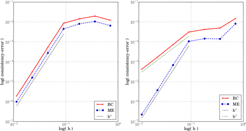
Figure 4: The consistency error is shown in a log-log plot for the Laplacian problem on the torus (cf. Fig. 5) for varying grid size of the control mesh and for the barycenter quadrature (BC) and the midedge quadrature (ME).

5 Numerical Applications

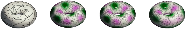
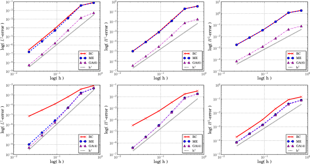
Figure 5: Results for the torus: in the first row from left to right we depict the subdivision limit surface with control lines, isolines and color coding of the right hand side $f(y)=\sin(\pi y_{1})\sin(\pi y_{2})\sin(\pi y_{3})$ ($-1.0$

$1.0$), the (numerical reference) solution of the Laplace-Beltrami problem ($-0.054$

$0.054$), and the (numerical reference) solution of the surface bi-Laplacian problem ($-0.003$

$0.003$) on $\mathcal{M}$; in the second and third row log-log plots of the error are reported for the Laplace-Beltrami problem ($2^{nd}$ row) and the surface bi-Laplacian problem ($3^{rd}$ row), respectively (from left to right: $L^{2}$-norm, $H^{1}$-semi-norm and $H^{2}$-semi-norm).

We have implemented the proposed methods in C++ and performed tests for four different subdivision surfaces: a torus surface with regular control mesh, a spherical surface (Spherical-3-4) with a control mesh with EVs of valence $3$ and $4$, a spherical surface (Spherical-5-12) with a control mesh with EVs of valence $5$ and $12$ and a complex real world hand model where the control mesh has altogether $119$ EVs of valence $4$, $5$, $7$, $8$, $9$ and $10$. Let us emphasize that, in the spirit of the isogeometric approach, the control mesh determining the limit subdivision geometry is kept fixed. Furthermore, the limit surface differs from a torus (Figure 5) with circular centerline and cross section or a perfect sphere (Figure 7). Then, we successively refine the control mesh using subdivision refinement to improve the accuracy of the discrete PDE solution. To run the simulations for Spherical-3-4, Spherical-5-12 and the hand model the initial control mesh has to be subdivided at least once to avoid EVs in direct neighborhood. In all tables, the mesh size $h$ refers to the mesh size of these control meshes.

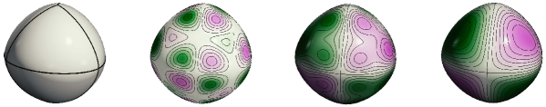
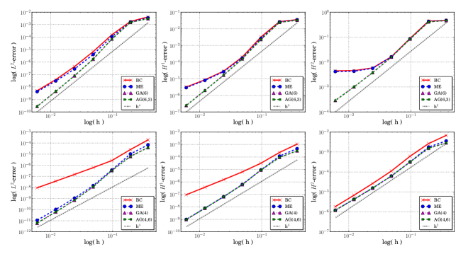
Figure 6: Results for Spherical-3-4: As in Figure 5 we show in the top row the limit surface, $f(y)=\sin(3\pi y_{1})\sin(3\pi y_{2})\sin(3\pi y_{3})$ ($-1.0$

$1.0$), the solution of the Laplace-Beltrami problem ($-5.25e-3$

$5.25e-3$), and the solution of the surface bi-Laplacian problem ($-9.78e-5$

$9.78e-5$), together with the error-plots for the Laplace-Beltrami problem ($2^{nd}$ row) and the surface bi-Laplacian problem ($3^{rd}$ row) (from left to right: $L^{2}$-norm, $H^{1}$-semi-norm and $H^{2}$-semi-norm).

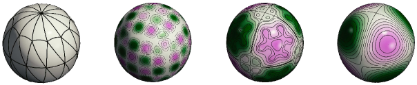
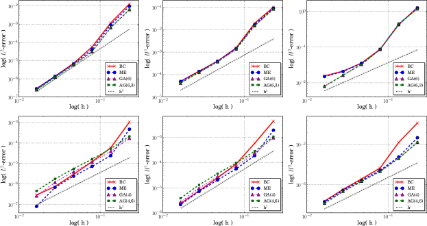
Figure 7: Results for Spherical-5-12: We follow the presentation in Fig. 6 and plot the limit surface with IgA-element lines, the (same) right hand side function $f$ now on this surface, the solution of the Laplace-Beltrami problem ($-1.58e-2$

$1.58e-2$), and the solution of the surface bi-Laplacian problem ($-1.27e-3$

$1.27e-3$), again together with the error-plots for the Laplace-Beltrami problem ($2^{nd}$ row) and the surface bi-Laplacian problem ($3^{rd}$ row) (from left to right: $L^{2}$-norm, $H^{1}$-semi-norm and $H^{2}$-semi-norm).

On all of these surfaces we solve the two model problems (1) and (2) for a given right-hand side $f$ and compare the asymptotic error for different norms: the $L^{2}$-norm, the $H^{1}$-semi-norm and the $H^{2}$-semi-norm. To evaluate the experimental order of convergence (eoc), we have computed a reference solution for a control mesh with one additional level of global refinement compared to the finest mesh. Furthermore to compute the reference solution we used the adaptive Gaussian quadrature AG($p$,$L$) with $L=3$ for (1) and for $L=6$ for (2) (the estimated convergence rates did not change for larger $L$). As a consequence, the error plots for the finest discretization are less reliable as it becomes apparent in Figure 7 for the $L^{2}$-error plot for problem (2) and the spherical shape with low valence EVs (Spherical-3-4). For all the experiments, double precision arithmetic is used.

Figure 5 shows our results for the torus with regular control mesh without EVs. All quadrature rules achieve optimal convergence rates (cf. [50]) for the second-order problem (1), i.e., $4$ in the $L^{2}$-norm, $3$ in the $H^{1}$-semi-norm and $2$ in the $H^{2}$-semi-norm (with non-adaptive Gaussian quadrature GA($p$)). Here, ”optimal” reflects what we expect for the quartic box spline [50]. For the fourth-order problem (2) all quadrature rules achieve optimal rates $4$ in the $L^{2}$-norm, $3$ in the $H^{1}$-semi-norm and $2$ in the $H^{2}$-semi-norm (with non-adaptive Gaussian quadrature GA($p$)), except the BC rule. Let us remark that the $C^{2}$-regularity allows for an Aubin-Nitzsche type argument [44] to obtain estimates in norms other than the energy norm. In all cases GA($p$) performed best.

The numerical results of the spherical control mesh with EVs of valence $3$ and $4$ (Spherical-3-4) depicted in Figure 6. For the second-order PDE (1) Gaussian quadrature and adaptive Gaussian quadrature achieve the optimal order of convergence. On finer resolutions ME and BC do not achieve optimal convergence rates. GA, AG and ME achieve similar behavior for the fourth-order problem and again the BC method performs worse. The reduced convergence rate in the $L^{2}$-norm for the fourth-order problem is expected to reflect the reduced regularity $C^{1}\cap H^{2}$, which precludes the application of an Aubin-Nitzsche type argument.

For the control mesh with EVs of valence $5$ and $12$ (Spherical-5-12) the convergence results are depicted in Figure 7 and coincide with our general findings for control meshes with EVs of valence greater than $6$. Here, all quadrature schemes show a similar performance, for the Laplace-Beltrami problem (1): $3$ in the $L^{2}$-norm, $2$ in the $H^{1}$-semi-norm and $1$ in the $H^{2}$-semi-norm, and for the surface bi-Laplacian problem (2) : $2$ in $L^{2}$-norm, $2$ in the $H^{1}$-semi-norm and $1$ in the $H^{2}$-semi-norm. This observed loss of approximation order compared to the quartic box spline coincides with the theoretical work by [27] with the reasoning that Loop subdivision functions cannot reproduce cubic polynomials around extraordinary vertices of valence greater then $6$.

Finally, we consider the hand model as a complex subdivision surface with many EVs in Figure 8. Given the complexity of the geometry and the number and valence of the extraordinary vertices both for the Laplace-Beltrami and surface bi-Laplacian problem the asymptotic regime of error reduction seems not to be reached even though the reference solution is computed on a mesh with $750k$ vertices. The BC fails for Bi-Laplacian probably caused by the increased number of EVs and their partially high valences. Figure 1 shows eigenfunctions of the Laplace-Beltrami operator computed via inverse vector iteration with projection. The depicted results underline that the methods discussed so far are also applicable in the numerical eigenmode analysis, which turned out to be an indispensable tool in geometric data analysis and modeling.

		GA($p$)		AG($p$,$L$)		BC		ME
Geometry	$\mid\mathcal{I}_{v}\mid$	$-\Delta_{\mathcal{M}}$	$(-\Delta_{\mathcal{M}})^{2}$	$-\Delta_{\mathcal{M}}$	$(-\Delta_{\mathcal{M}})^{2}$	$-\Delta_{\mathcal{M}}$	$(-\Delta_{\mathcal{M}})^{2}$	$-\Delta_{\mathcal{M}}$	$(-\Delta_{\mathcal{M}})^{2}$
Spherical-5-12	9218	1.209	1.417	1.374	1.563	0.164	0.272	0.107	0.136
Hand	11586	1.914	2.233	2.615	3.424	0.269	0.460	0.157	0.198

Table 2: Comparison of assembly times for the stiffness matrices (10) and (11) and the different quadrature rules (Gaussian GA($p$), adaptive Gaussian AG($p$,$L$), barycenter (BC) and mid-edge (ME)). All times reported in seconds.

Compared to Gaussian quadrature and in particular to the adaptive Gaussian quadrature the mid-edge and the barycenter quadrature are significantly cheaper as reported in Table 2. Because of our implementation, the mid-edge rule based on lookup tables and assembly via an edge-iterator performs even better than the (non-optimized) barycenter rule.

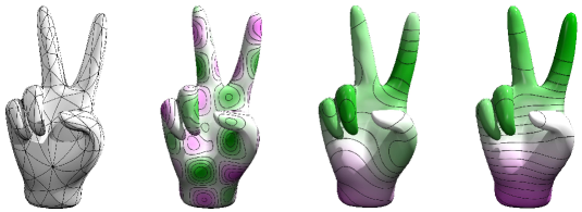
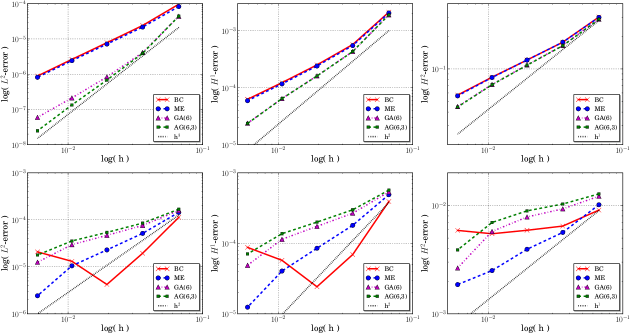
Figure 8: Results for complex hand shape: We follow the presentation in Fig. 6 and plot the limit surface with IgA-element lines, the (same) right hand side function $f$ now on this surface, the solution of the Laplace-Beltrami problem ($-1.47e-2$

$1.14e-2$) and the solution of the surface bi-Laplacian problem ($-8.14e.4$

$7.56e.4$), again together with the error-plots for the Laplace-Beltrami problem ($2^{nd}$ row) and the surface bi-Laplacian problem ($3^{rd}$ row) (from left to right: $L^{2}$-norm, $H^{1}$-semi-norm and $H^{2}$-semi-norm).

6 Conclusions

We have explored the discretizations of geometric partial differential equations on subdivision surfaces by means of an isogeometric approach. To this end, we have focused on Loop’s subdivision method and have investigated the impact of different numerical quadrature rules on the expected convergence rates. As expected, there is a trade-off between robustness and computational effort. The adaptive Gaussian quadrature turns out to be the most robust in the carefully selected set of test cases but at the same time computationally demanding for instance for real-time applications in modeling and animation. In fact, the mid-edge quadrature based on lookup tables has been singled out as a promising compromise for both graphics and engineering applications. It is very easy to implement and it performed well in all considered test cases. Fourth-order problems like the surface bi-Laplacian problem considered here, are by far more critical with respect to the accuracy of the numerical approximation than second-order problems. In general, adaptivity around EVs is essential to ensure the overall robustness on very fine computational meshes.

References

- [1] T. Hughes, J. Cottrell, Y. Bazilevs, Isogeometric analysis: CAD, finite elements, NURBS, exact geometry and mesh refinement, Computer Methods in Applied Mechanics and Engineering 194 (39–41) (2005) 4135–4195.
- [2] J. A. Cottrell, T. J. R. Hughes, Y. Bazilevs, Isogeometric Analysis: Toward Integration of CAD and FEA, John Wiley & Sons, Chichester, England, 2009.
- [3] P. Antolin, A. Buffa, F. Calabro, M. Martinelli, G. Sangalli, Efficient matrix computation for tensor-product isogeometric analysis: The use of sum factorization, Computer Methods in Applied Mechanics and Engineering 285 (2015) 817 – 828.
- [4] T. Hughes, A. Reali, G. Sangalli, Efficient quadrature for NURBS-based isogeometric analysis, Computer Methods in Applied Mechanics and Engineering 199 (5–8) (2010) 301–313.
- [5] A. Mantzaflaris, B. Jüttler, Integration by Interpolation and Look-up for Galerkin-based Isogeometric Analysis, Computer Methods in Applied Mechanics and Engineering 284 (2015) 373–400, Isogeometric Analysis Special Issue.
- [6] A. Mantzaflaris, B. Jüttler, B. Khoromskij, U. Langer, Matrix Generation in Isogeometric Analysis by Low Rank Tensor Approximation, Tech. rep., NFN G+S: Technical Report No. 19 (2014).
- [7] D. Schillinger, S. Hossain, T. Hughes, Reduced Bézier element quadrature rules for quadratic and cubic splines in isogeometric analysis, Computer Methods in Applied Mechanics and Engineering 277 (2014) 1–45.
- [8] J. Peters, U. Reif, Subdivision Surfaces, Springer Series in Geometry and Computing, 2008.
- [9] T. J. Cashman, Beyond Catmull-Clark? A survey of advances in subdivision surface methods, Computer Graphics Forum 31 (1) (2012) 42–61.
- [10] T. DeRose, M. Kass, T. Truong, Subdivision Surfaces in Character Animation, in: Proceedings of the 25th Annual Conference on Computer Graphics and Interactive Techniques, SIGGRAPH ’98, 1998, pp. 85–94.
- [11] B. Thomaszewski, M. Wacker, W. Straßer, A Consistent Bending Model for Cloth Simulation with Corotational Subdivision Finite Elements, in: Proceedings of the 2006 ACM SIGGRAPH/Eurographics Symposium on Computer Animation, SCA ’06, 2006, pp. 107–116.
- [12] F. Cirak, M. Ortiz, P. Schröder, Subdivision surfaces: a new paradigm for thin-shell finite-element analysis, International Journal for Numerical Methods in Engineering 47(12) (2000) 2039–72.
- [13] F. Cirak, Q. Long, Subdivision shells with exact boundary control and non-manifold geometry, International Journal for Numerical Methods in Engineering 88(9) (2011) 897–923.
- [14] F. Cirak, M. Scott, E. Antonsson, M. Ortiz, P. Schröder, Integrated modeling, finite-element analysis and engineering design for thin-shell structures using subdivision, Computer-Aided Design 34(2) (2002) 137–148.
- [15] F. Cirak, M. Ortiz, Fully C1-conforming subdivision elements for finite deformation thin-shell analysis, International Journal for Numerical Methods in Engineering 51(7) (2001) 813–833.
- [16] S. Green, G. Turkiyyah, D. Storti, Subdivision-Based Multilevel Methods for Large Scale Engineering Simulation of Thin Shells, in: Proceedings of ACM Solid Modeling, 2002.
- [17] S. Green, G. Turkiyyah, Second Order Accurate Constraint Formulation for Subdivision Finite Element Simulation of Thin Shells, International Journal For Numerical Methods In Engineering 61 (3) (2004) 380–405.
- [18] M. Antonelli, C. Beccari, G. Casciola, R. Ciarloni, S. Morigi, Subdivision surfaces integrated in a CAD system, Computer-Aided Design 45 (2013) 1294–1305.
- [19] I. Boier-Martin, D. Zorin, Differentiable Parameterization of Catmull-Clark Subdivision Surfaces, in: Proceedings of the 2004 Eurographics/ACM SIGGRAPH Symposium on Geometry Processing, SGP ’04, ACM, New York, NY, USA, 2004, pp. 155–164.
- [20] E. Catmull, J. Clark, Recursively generated B-spline surfaces on arbitrary topological meshes, Computer Aided Design 10 (1978) 350–355.
- [21] D. Doo, M. Sabin, Behaviour of recursive division surfaces near extraordinary points, Computer-Aided Design 10(6) (1978) 356–360.
- [22] C. Loop, Smooth spline surfaces over irregular meshes, in: SIGGRAPH ’94: Proceedings of the 21st annual conference on Computer graphics and interactive techniques, ACM Press, 1994, pp. 303–310.
- [23] U. Reif, A unified approach to subdivision algorithms near extraordinary vertices, Computer Aided Geometric Design 12 (1995) 153–174.
- [24] U. Reif, P. Schröder, Curvature integrability of subdivision surfaces, Advances in Computational Mathematics 14(2) (2001) 157–174.
- [25] J. Peters, X. Wu, On the local linear independence of generalized subdivision functions, SIAM Journal on Numerical Analysis (SINUM) 44 (6) (2006) 2389–2407.
- [26] U. Zore, B. Jüttler, J. Kosinka, On the Linear Independence of (Truncated) Hierarchical Subdivision Splines, Tech. rep., NFN G+S: Technical Report No. 17 (2014).
- [27] G. Arden, Approximation properties of subdivision surfaces, Ph.D. thesis, University of Washington (2001).
- [28] J. Stam, Evaluation of Loop Subdivision Surfaces, Computer Graphics Proceedings (SIGGRAPH 1999).
- [29] E. Grinspun, P. Krysl, P. Schröder, CHARMS: A Simple Franmework for Adaptive Simulation, in: Computer Graphics (SIGGRAPH ’02 Proceedings), 2002.
- [30] C. Bajaj, G. Xu, Anisotropic Diffusion of Subdivision Surfaces and Functions on Surfaces, ACM Transactions on Graphics 22 (1) (2003) 4–32.
- [31] U. Clarenz, U. Diewald, M. Rumpf, Processing textured surfaces via anisotropic geometric diffusion, IEEE Transactions on Image Processing 13 (2) (2004) 248–261.
- [32] K. Hildebrandt, K. Polthier, Anisotropic Filtering of Non-Linear Surface Features, Eurographics 23 (3).
- [33] L. Dede, A. Quarteroni, Isogeometric Analysis for second order Partial Differential Equations on surfaces, Computer Methods in Applied Mechanics and Engineering 284 (2015) 807–834.
- [34] U. Langer, A. Mantzaflaris, S. E. Moore, I. Toulopoulos, Multipatch Discontinuous Galerkin Isogeometric Analysis, Tech. rep., NFN G+S: Technical Report No. 18 (2014).
- [35] U. Langer, S. E. Moore, Discontinuous Galerkin Isogeometric Analysis of Elliptic PDEs on Surfaces, Tech. rep., NFN G+S: Technical Report No. 12 (2014).
- [36] P. J. Barendrecht, Isogeometric Analysis for Subdivision Surfaces, Master’s thesis, Eindhoven University of Technology (2013).
- [37] A. Wawrzinek, K. Hildebrandt, K. Polthier, Koiter’s Thin Shells on Catmull-Clark Limit Surfaces, in: P. Eisert, J. Hornegger, K. Polthier (Eds.), VMV 2011: Vision, Modeling & Visualization, Eurographics Association, 2011, pp. 113–120. doi:10.2312/PE/VMV/VMV11/113-120.
- [38] E. Dikici, S. R. Snare, F. Orderud, Isoparametric Finite Element Analysis for Doo-Sabin Subdivision Models, in: Proceedings of Graphics Interface 2012, GI ’12, 2012, pp. 19–26.
- [39] D. Burkhart, B. Hamann, G. Umlauf, Iso-geometric analysis based on Catmull-Clark solid subdivision, Computer Graphics Forum 29 (5) (2010) 1575–1784.
- [40] C. Loop, Smooth subdivision surfaces based on triangles, Master’s thesis (1987).
- [41] E. Stollnitz, A. DeRose, D. Salesin, Wavelets for Computer Graphics: Theory and Applications, Morgan Kaufmann, 1996.
- [42] S. C. Brenner, L. R. Scott, The mathematical theory of Finite Element methods, Springer-Verlag, 2002.
- [43] D. Braess, Finite Elements, 3rd Edition, Cambridge University Press, 2007.
- [44] P. G. Ciarlet, The finite element method for elliptic problems, no. 40 in Classics in applied mathematics, SIAM, 2002.
- [45] G. Dziuk, Finite elements for the Beltrami operator on arbitrary surfaces, in: S. Hildebrandt, R. Leis (Eds.), Partial Differential Equations and Calculus of Variations, Lecture Notes in Mathematics 1357, Springer, 1988, pp. 142–155.
- [46] R. Schaback, H. Werner, Numerische Mathematik, 4th Edition, Springer, 1992.
- [47] D. A. Dunavant, High degree efficient symmetrical Gaussian quadrature rules for the triangle, Int. J. Numer. Meth. Engng 21 (1985) 1129–1148.
- [48] L. Kobbelt, K. Daubert, H. Seidel, Ray Tracing of Subdivision Surfaces, in: Rendering Techniques ’98, Proceedings of the Eurographics Workshop in Vienna, Austria, June 29 - July 1, 1998, 1998, pp. 69–80.
- [49] G. Strang, G. J. Fix, An Analysis of the Finite Element Method, Prentice-Hall, Englewood Cliffs, N.J., 1973.
- [50] J. K. Kowalski, Application of Box Splines to the Approximation of Sobolev Spaces, J. Approx. Theory 61 (1990) 53–73.