Probing small-scale non-Gaussianity from anisotropies in acoustic reheating

Abstract

We give new constraints on small-scale non-Gaussianity of primordial curvature perturbations by the use of anisotropies in acoustic reheating. Mixing of local thermal or local kinetic equilibrium systems with different temperatures yields a locally averaged temperature rise, which is proportional to the square of temperature perturbations damping in the photon diffusion scale. Such secondary temperature perturbations are indistinguishable from the standard temperature perturbations linearly coming from primordial curvature perturbations and hence should be subdominant compared to the standard ones. We show that small-scale higher order correlation functions (connected non-Gaussian and disconnected Gaussian parts) of primordial curvature perturbations can be probed by investigating auto power spectrum of the generated secondary perturbations and the cross power spectrum with the standard perturbations. This is simply because these power spectra come from higher order correlation functions of primordial curvature perturbations with non-linear parameters such as $f_{\rm NL}$ and $\tau_{\rm NL}$ since secondary temperature perturbations are second order effects. Thus, the observational results $l(l+1)C^{TT}_{l}\simeq 6\times 10^{-10}$ at large scales give a robust and universal upper bound on small-scale non-Gaussianities of primordial curvature perturbations.

1 Introduction

The 21st century is the age of precise observational cosmology. It is possible to observationally test theoretical models for the early universe by analysing anisotropies of the Cosmic Microwave Background (CMB) [1, 2]. In fact, we already know that primordial curvature perturbations do exist, and their spectrum is almost scale-invariant. While the statistical property of primordial perturbations is well approximated by Gaussian statistics, the deviation from the exact Gaussian statistics [3] will deliver us rich information on the primordial universe [4], which is one of the next targets in cosmology. On the other hand, it should be noticed that the scales probed by the CMB anisotropies are just $6$ $e$-foldings of the last $60$ $e$-folds during inflation and that we know very little about smaller-scale perturbations on $k~{}{\rm Mpc}\gtrsim 0.1$ because most of the primordial density fluctuations dissipate due to Silk damping. One powerful tool to see the fluctuations on small scales is CMB spectral distortions [5, 6, 7, 8, 9, 10, 11, 12, 13]. Deviations from the ideal blackbody spectrum are induced in the early universe after around $z\simeq 2\times 10^{6}$, and such deviations are characterized in terms of several parameters such as the Compton $y$ parameter and the chemical potential $\mu$. The next observational projects, such as PIXIE and PRISM [14, 15], following COBE/FIRAS are proposed [16, 17, 18], and it may be possible to see the nature of primordial fluctuations up to another $11$ $e$-foldings in the near future. Hence, $17$ $e$-foldings will be within the scope of our current technology, but more than one half of total $e$-foldings necessary to solve the initial condition problems remain obscure.

Recently, acoustic reheating was proposed to investigate primordial curvature perturbations on extremely small scales [19, 20]. Below the diffusion scale, the inhomogeneities are erased due to Silk damping so that the universe is heated by the conversion of the dissipated energy of photon [21]. Such temperature rises are quadratic in temperature fluctuations over the diffusion scale. In the previous works, the total average (homogeneous part) of the temperature rise was discussed, and they derived the constraints on small-scale power spectrum of primordial curvature perturbations by comparing the helium mass fraction ${\rm Y}_{p}$ (or photon baryon ratio $\eta_{B}$) during Big Bang nucleosynthesis with that at the last scattering of the CMB. Such investigations are new and interesting, but the scales probed by these approaches are limited up to $k{\rm Mpc}\simeq\mathcal{O}(10^{5})$ since the heating in much smaller scales (at much earlier epochs) changes both $\eta^{\rm BBN}_{B}$ and $\eta^{\rm CMB}_{B}$, so that we know very little about the scale except the constraints that $\mathcal{P}_{\mathcal{R}}\lesssim 0.3$ for $k\sim 10^{20-25}{\rm Mpc}^{-1}$ [19]. However, the temperature rise induced by acoustic reheating is only homogenized over the diffusion scale. Then, it fluctuates spatially in general and potentially includes all of the histories of erased temperature perturbations from the beginning of the hot universe, that is, if large inhomogeneities would exist at small scales, the observed temperature anisotropies can be changed drastically. In this paper, we shall focus on such inhomogeneities of acoustic reheating. Although one cannot pick up and isolate the temperature perturbations due to acoustic reheating from the observed temperature anisotropies, given the fact that the linear theory prediction well matches with the CMB observations, the non-linear corrections should not be beyond the observational $C^{TT}_{l}$, i.e. the order of $10^{-10}$ at large scales. This puts robust and universal constraints on higher order correlation functions including non-Gaussianities of primordial curvature perturbations since the non-linear temperature corrections are of the second order of primordial curvature perturbations. Our approach is closely related with a method to investigate anisotropies in CMB distortions which was originally proposed by Pajer and Zaldarriaga since the physics of acoustic reheating is essentially the same [22].

We organize this paper as follows. In section 2, we summarize the details of acoustic reheating, particularly paying attention to its perturbations. Section 3 and 4 are devoted to the calculations of angular power spectrum by the use of Sachs-Wolfe approximation, and we obtain the constraints on the non-Gaussianities of primordial curvature perturbations in section 5. We give conclusions and discussions in the final section, and scale-dependence of non-Gaussianities is briefly mentioned in the appendix.

2 Inhomogeneities in acoustic reheating

The local photon temperature in the early universe fluctuates due to the primordial curvature perturbations. As long as the Compton and the double-Compton processes are efficient, which holds for $z\gtrsim 2\times 10^{6}$ [23, 24], it is locally in thermal equilibrium, and its spectrum obeys the Planck distribution characterized only by the local temperature $T(\eta,\mbox{\boldmath${x}$},\hat{\mbox{\boldmath${n}$}})$, where $\eta$, ${x}$ and $\hat{\mbox{\boldmath${n}$}}$ are the conformal time, the space coordinate and the unit vector of the photon momentum respectively. This local temperature can be divided into the homogeneous part and the inhomogeneous one,

$$T(\eta,\mbox{\boldmath${x}$},\hat{\mbox{\boldmath${n}$}})=\overline{T}(\eta)\bigl{(}1+\Theta(\eta,\mbox{\boldmath${x}$},\hat{\mbox{\boldmath${n}$}})\bigr{)}.$$ (2.1)

Here, the acoustic reheating is not yet taken into account, and hence $\overline{T}$ decreases in proportional to $a(\eta)^{-1}$ ($a(\eta)$ : the scale factor) in the expanding Universe as long as the number of the effective degree of freedom of radiations is unchanged, and the temperature perturbations are proportional to the primordial curvature perturbations at linear order. Once the acoustic reheating happens, small-scale inhomogeneities are erased due to Silk damping, and the effective temperature is raised because of the energy conservation. Now, let us evaluate the temperature rise for a given perturbed system of photons, assuming acoustic reheating happens instantaneously. Keeping in mind the relation between the temperature and the energy density of photons $\rho$, $T=(\rho/a_{B})^{1/4}$ with the numerical constant $a_{B}=\pi^{2}/15$, the dimensionless temperature rise $\Delta$ is given by

$$\Delta(\mbox{\boldmath${x}$})=\frac{\langle\rho\rangle^{\frac{1}{4}}_{\bm{x}}-\langle\rho^{\frac{1}{4}}\rangle_{\bm{x}}}{\bar{T}},$$ (2.2)

where $\langle X\rangle_{\bm{x}}$ represents a spacial average defined as

$$\langle X\rangle_{\bm{x}}=\int d^{3}\mbox{\boldmath${x}$}^{\prime}~{}W_{r_{T}}(\bm{x}^{\prime})X(\bm{x}+\bm{x}^{\prime})$$ (2.3)

with $W_{r_{T}}$ being a window function with a radius $r_{T}$ around $\bm{x}$. This spacial averaging procedure effectively represents the (instantaneous) acoustic reheating, in which we assume that damping and thermalization happen instantaneously within the same box. The term $\langle\rho\rangle^{\frac{1}{4}}_{\bm{x}}$ represents the average temperature when the energy density of photons around ${\bm{x}}$ would be damped perfectly and thermalized homogeneously within the radius $r_{T}$. Another term $\langle\rho^{\frac{1}{4}}\rangle_{\bm{x}}$ represents the average temperature when the (fluctuating) photon temperature would be homogenized within the radius $r_{T}$. From the energy conservation, this difference yields the temperature rise. One can easily see that this effect comes from nonlinear relation between the energy density and the temperature of photons, and is second order in perturbations of the photon temperature. In fact, inserting the definition of the photon perturbation (2.1) into (2.2) yields $\Delta(\bm{x})=3\langle\Theta_{i}^{2}\rangle_{\bm{x}}/2$. Here $\Theta_{i}$ represents the temperature perturbation before acoustic reheating happens. Realistic acoustic reheating proceeds through two processes, damping of the photon perturbations due to Silk damping followed by (homogeneously) thermalization through the Compton and the double-Compton processes. Therefore, the actual temperature rise for a conformal time $\eta$ can be written as

$$\Delta(\eta,\mbox{\boldmath${x}$})=\frac{3}{2}\langle\Theta_{i}^{2}-\Theta^{2}(\eta)\rangle_{\mbox{\boldmath${x}$}}.$$ (2.4)

Here, we separate two processes explicitly. $\Theta_{i}^{2}-\Theta^{2}(\eta)$ represents only the damping effect and includes the time evolution of damping scales. The spacial average in this equation represents only (homogeneous) thermalization effect and does not include the damping effect. Then, this equation can be recast into the evolution equation of $\Delta$ as

$$\frac{d\Delta}{d\eta}=-\frac{3}{2}\frac{d\langle\Theta^{2}\rangle_{\bm{x}}}{d\eta}.$$ (2.5)

Strictly speaking, thermalization (diffusion) radius $r_{T}$ also depends on the conformal time. However, as long as we are interested in the final temperature rise, we have only to take $r_{T}$ to be the largest thermalization radius during acoustic reheating. Therefore, we fix $r_{T}$ to be such a radius here and hereafter.

During $5\times 10^{4}<z<2\times 10^{6}$, the double Compton process is negligible while the Compton process is still efficient. Then, the system is locally in kinetic equilibrium, but its spectrum obeys the Bose-Einstein distribution with a nonzero chemical potential $\mu$ [23, 25, 24], which modifies the expression of the temperature rise $\Delta$ for a given perturbed system of photons, assuming acoustic reheating happens perfectly and instantaneously, as

$$\Delta=\frac{\langle\rho\rangle^{\frac{1}{4}}_{\bm{x}}-\langle\rho^{\frac{1}{4}}\rangle_{\bm{x}}}{\bar{T}}-\frac{45\zeta(3)}{2\pi^{4}}\langle\mu\rangle_{\bm{x}},$$ (2.6)

with $\zeta$ being a Riemann zeta function. Subtraction of the chemical potential means that the temperature of the Bose-Einstein system is not the forth root of the energy density. Then, the relation between the temperature rise, and the photon perturbation is also modified as [13]

$$\frac{d\Delta}{d\eta}\simeq-2.277\frac{d\langle\Theta^{2}\rangle_{\bm{x}}}{d\eta}.$$ (2.7)

Thus, in order to estimate the amount of the acoustic reheating, we have only to evaluate how much the temperature perturbations originated from the primordial curvature perturbations decay due to Silk damping. Once the acoustic reheating is taken into account, the local temperature is modified from (2.1) into

$$T(\eta,\mbox{\boldmath${x}$},\hat{\mbox{\boldmath${n}$}})=\overline{T}(\eta)\bigl{[}1+\Theta(\eta,\mbox{\boldmath${x}$},\hat{\mbox{\boldmath${n}$}})+\Delta(\eta,\mbox{\boldmath${x}$})\bigr{]}.$$ (2.8)

It should be noticed that $\Delta$ consists of only a monopole component because of the thermalization effects and that it will include the homogeneous part for the entire Universe in general, which can reheat the whole Universe.

The time evolution of the linear temperature perturbations in the conformal Newtonian gauge is described by the Boltzmann equation [26, 27, 28, 29],

$$\frac{d}{d\eta}\Theta=\dot{\phi}-(\mbox{\boldmath${\hat{k}}$}\cdot\mbox{\boldmath${\hat{n}}$})\psi+\dot{\tau}\left[\Theta-\Theta_{0}+\frac{1}{2}P_{2}(\mbox{\boldmath${\hat{k}}$}\cdot\mbox{\boldmath${\hat{n}}$})(\Theta_{2}+\Theta^{P}_{2}+\Theta^{P}_{0})-(\mbox{\boldmath${\hat{k}}$}\cdot\mbox{\boldmath${\hat{n}}$})v\right],$$ (2.9)

where $\tau$ is the optical depth, and $\mbox{\boldmath${\hat{k}}$}\cdot\mbox{\boldmath${\hat{n}}$}$ is a cosine between unit vectors of the photon momentum and the Fourier momentum. Over-dots represent partial derivatives with respect to the conformal time. Each quantity is Fourier transformed, and $\Theta$ is also expanded by Legendre polynomials $P_{l}$ as $\Theta=\sum_{l}(-i)^{l}(2l+1)P_{l}(\hat{k}\cdot\hat{n})\Theta_{l}$. $\Theta^{P}$ is the polarization, and its Legendre coefficients are given in the same manner. The definitions of the velocity potential $v$, gravitational potential $\psi$ and the curvature perturbation $\phi$ are based on [28]. The third term on the r.h.s. is negligible on large scales. Then, the monopole and the dipole components of temperature perturbations are enhanced due to the Sachs-Wolfe effects just after the horizon entry. Once $\phi$ and $\psi$ decay, the monopole and the dipole oscillate in the inverted phase. The leading term proportional to $\dot{\tau}$ comes from the quadrupole component, and emerging of such nonzero anisotropic stress induces the diffusion damping. Below the diffusion scale, the Boltzmann hierarchies are solved approximately [30],

$$\Theta_{1}\simeq-\frac{1}{\sqrt{3}}\sin(kr_{s})\exp\left(-\frac{k^{2}}{k_{D}^{2}}\right)\mathcal{R}_{\bm{k}},$$ (2.10)

where $\mathcal{R}_{\bm{k}}$ is primordial curvature perturbations on comoving slice, $k_{D}^{-1}$ corresponds to the diffusion scale, and $r_{s}$ is the sound horizon. In the quasi tight coupling regime, the following relations approximately hold, $\Theta^{P}_{2}+\Theta^{P}_{0}=\frac{3}{2}\Theta_{2}$, $\Theta_{2}=8k\Theta_{1}/(15\dot{\tau})$ and $\partial_{\eta}k^{-2}_{D}=-8/(45\dot{\tau})$. As pointed in [19], the diffusion scale should be divided into at least $5$ regions depending on redshift dependence of $k_{D}$ and the chemical potential. Taking the beginning of the hot universe to be $z_{0}=10^{30}$, in which anisotropic shear comes from relativistic species such as $\gamma$, $W^{\pm}$ and $Z$ bosons until $z_{1}\sim 1.5\times 10^{14}$, damping scale is written as $k_{D}\simeq 5.5\times 10^{9}(1+z)^{0.51}{\rm Mpc}^{-1}$. Once the weak bosons acquire their masses, neutrino is a dominant component to smooth inhomogeneities before neutrino decoupling around $z_{2}\sim 5.5\times 10^{9}$, and the diffusion scale is given by $k_{D}\simeq 5.0\times 10^{-22}(1+z)^{2.7}{\rm Mpc}^{-1}$. Since neutrino can smooth inhomogeneities over the whole horizon scale just before the decoupling, the diffusion scale is almost the same with that at decoupling. Then, the diffusion scale is almost constant until the photon diffusion scale goes beyond $k_{D}\simeq 10^{5}{\rm Mpc}^{-1}$ around $z_{3}\sim 8.4\times 10^{6}$. $z_{5}\simeq 5\times 10^{4}$ is the lower bound since kinetic equilibrium is not established anymore. Thus, during $z_{5}<z<z_{3}$, the damping scale is induced by photon diffusion and is written as $k_{D}\simeq 4.1\times 10^{-6}(1+z)^{3/2}{\rm Mpc}^{-1}$. Though the diffusion scale is unchanged, we need to distinguish a chemical potential era from a blackbody era, whose transition happens around $z_{4}\simeq 2\times 10^{6}$. Combining (2.5), (2.9), and (2.10), the temperature rise in the Newton gauge due to the acoustic reheating at the last scattering conformal time $\eta_{\ast}$ is evaluated as

$$\Delta(\eta_{\ast},\mbox{\boldmath${x}$})= 2\int\frac{d^{3}\mbox{\boldmath${k_{1}}$}}{(2\pi)^{3}}\frac{d^{3}\mbox{\boldmath${k_{2}}$}}{(2\pi)^{3}}e^{i(\bm{k}_{1}+\bm{k}_{2})\cdot\bm{x}}\mathcal{W}_{r_{T}}(k)5P_{2}(\mbox{\boldmath${\hat{k}}$}_{1}\cdot\mbox{\boldmath${\hat{n}}$})P_{2}(\mbox{\boldmath${\hat{k}}$}_{2}\cdot\mbox{\boldmath${\hat{n}}$})\langle\sin(k_{1}r_{s})\sin(k_{2}r_{s})\rangle_{p}$$

$$\times\sum^{5}_{n=1}\alpha_{n}\left[\exp{\left(-\frac{k_{1}^{2}+k_{2}^{2}}{k^{2}_{D}(z)}\right)}\right]^{z_{n-1}}_{z_{n}}\mathcal{R}_{\bm{k}_{1}}\mathcal{R}_{\bm{k}_{2}},$$ (2.11)

where $\langle\cdots\rangle_{p}$ is periodic average over the duration longer than the oscillation period. $z_{n}$ and $\alpha_{n}$ is given by $(z_{0},\cdots,z_{5})=(10^{30},1.5\times 10^{14},5.5\times 10^{9},8.4\times 10^{6},2\times 10^{6},5\times 10^{4})$ and $(\alpha_{1},\cdots,\alpha_{4},\alpha_{5})=(3/2,\cdots,3/2,2.28)$, respectively. In (2.11), we drop the dipole contribution proportional to $\Theta_{1}\dot{\Theta}_{1}P_{1}(\hat{k}_{1})P_{1}(\hat{k}_{2})$ because its periodic average vanishes, and omitted the higher order multipoles proportional to $P_{l}P_{l^{\prime}}$ with $l\neq l^{\prime}$, which vanish thanks to the orthogonality of the Legendre polynomials when we estimate the angular power spectrum later. Coarse graining is operated through the window function $\mathcal{W}_{r_{T}}(k)$, which is the Fourier transformation of $W_{r_{T}}(\bm{x})$ defined in (2.3). The typical scale of such homogenization is given by the maximum scale of thermalization around $z\simeq 5\times 10^{4}$. Then, inhomogeneities in acoustic reheating are erased on scales below $\mathcal{O}(0.1{\rm Mpc})$.

In Fourier space, (2.11) can be written as

$$\Delta(\eta_{\ast},\mbox{\boldmath${k}$})= 2\sum^{5}_{n=1}\alpha_{n}\int\frac{d^{3}\mbox{\boldmath${k}$}_{1}}{(2\pi)^{3}}\int\frac{d^{3}\mbox{\boldmath${k}$}_{2}}{(2\pi)^{3}}5P_{2}(\mbox{\boldmath${\hat{k}}$}_{1}\cdot\mbox{\boldmath${\hat{n}}$})P_{2}(\mbox{\boldmath${\hat{k}}$}_{2}\cdot\mbox{\boldmath${\hat{n}}$})(2\pi)^{3}\delta^{(3)}(\mbox{\boldmath${k}$}-\mbox{\boldmath${k}$}_{1}-\mbox{\boldmath${k}$}_{2})$$

$$\mathcal{W}_{r_{T}}(k)\langle\sin(k_{1}r_{s})\sin(k_{2}r_{s})\rangle_{p}\left[\exp\left(-\frac{k_{1}^{2}+k_{2}^{2}}{k_{D}^{2}(z)}\right)\right]^{z_{n-1}}_{z_{n}}\mathcal{R}_{\bm{k}_{1}}\mathcal{R}_{\bm{k}_{2}}.$$ (2.12)

Here, it should be noticed that the temperature rise due to acoustic reheating is smoothed over the diffusion radius $r_{T}$, so that the contribution for $k\gg r_{T}^{-1}$ is significantly suppressed. However, this fact implies that only the sum of $\mbox{\boldmath${k}$}_{1}$ and $\mbox{\boldmath${k}$}_{2}$ must be small and that $k_{1}$ and $k_{2}$ themselves can be large because the acoustic reheating is the second order effect. This is the essential reason why the perturbations of acoustic reheating can probe the information of primordial curvature perturbations on small scales.

Before the end of this section, we shall make a comment on the other $2$nd order effects. In the above $\Theta$ is assumed to be given by the solution of the linearized Boltzmann equation, (2.9). As studied in [31, 32, 33, 34, 35], the non-linearity of the Boltzmann and the Einstein equations also induces non-linear temperature fluctuations of the CMB, namely the non-linear part of $\Theta$. While such $2$nd order effects are so far evaluated around and after the recombination, we investigate a part of such $2$nd order effects generated well before the recombination in this paper. Then the effect estimated in this paper will be separately treated from the standard $2$nd order effects simply because the physical origin is different. Of course, in order to compare with the observed temperature anisotropies of the CMB, one should take into account the both effects, which are indistinguishable in fact. Here, to emphasize and note the importance of $2$nd order effects well before the recombination, we shall especially focus on this part of specific $2$nd order effects.

3 Angular power spectrum

Temperature anisotropies which we observe are decomposed using the spherical Harmonics $Y_{lm}$, and their coefficients are defined as

$$a^{\Theta}_{lm} =\int d\mbox{\boldmath${\hat{n}}$}Y^{*}_{lm}(\mbox{\boldmath${\hat{n}}$})\Theta(\bm{x}=0,\mbox{\boldmath${\hat{n}}$}),$$ (3.1)

$$a^{\Delta}_{lm} =\int d\mbox{\boldmath${\hat{n}}$}Y^{*}_{lm}(\mbox{\boldmath${\hat{n}}$})\Delta(\bm{x}=0,\mbox{\boldmath${\hat{n}}$}),$$ (3.2)

where we have set the coordinate of an observer to the origin without loss of generality. $\Theta$ and $\Delta$ above are evolved from the last scattering surface and hence $\Delta$ has $\hat{\mbox{\boldmath${n}$}}$ dependence as well in contrast to (2.11). The coefficient of the total temperature perturbations is given by $a^{T}_{lm}=a^{\Theta}_{lm}+a^{\Delta}_{lm}$. Then, the CMB temperature angular correlation is written as $C^{TT}_{l}=C^{\Theta\Theta}_{l}+2C^{\Theta\Delta}_{l}+C^{\Delta\Delta}_{l}$, where we have defined

$$C^{XY}_{l}=\frac{1}{2l+1}\sum_{m=-l}^{l}\langle a^{X*}_{lm}a^{Y}_{lm}\rangle,$$ (3.3)

and $\langle\cdots\rangle$ represents the ensemble average. From the observations of the CMB anisotropies, $C_{l}^{TT}$ at large scales are known to be the order of $\mathcal{O}(10^{-10})$. Therefore, unless each contribution cancels out accidentally, it should be smaller than $\mathcal{O}(10^{-10})$, that is, $C^{\Theta\Delta}_{l}\lesssim\mathcal{O}(10^{-10})$ and $C^{\Delta\Delta}_{l}\lesssim\mathcal{O}(10^{-10})$. These conditions yield new constraints on the primordial curvature perturbations at small scales. This is the central topic of this paper.

Using the Fourier modes, we can express (3.1) and (3.2) as

$$a^{\Theta}_{lm} =4\pi(-i)^{l}\int\frac{d^{3}\mbox{\boldmath${k}$}}{(2\pi)^{3}}Y^{*}_{lm}(\mbox{\boldmath${\hat{k}}$}){\cal T}_{l}(k,\eta_{0})\Theta(\eta_{\ast},\mbox{\boldmath${k}$}),$$ (3.4)

$$a^{\Delta}_{lm} =4\pi(-i)^{l}\int\frac{d^{3}\mbox{\boldmath${k}$}}{(2\pi)^{3}}Y^{*}_{lm}(\mbox{\boldmath${\hat{k}}$}){\cal T}_{l}(k,\eta_{0})\Delta(\eta_{\ast},\mbox{\boldmath${k}$}),$$ (3.5)

where $\eta_{0}$ is the present conformal time. The transfer function is given by ${\cal T}_{l}\simeq[\Theta_{0}(\eta_{*})+\Psi(\eta_{*})]j_{l}[k(\eta_{0}-\eta_{*})]\simeq-3j_{l}(k\eta_{0})/5$. We can use the same transfer function for $\Theta$ and $\Delta$ because they are indistinguishable. Using a relation between spherical harmonics and Legendre polynomials

$$\sum^{l}_{m=-l}Y^{*}_{lm}(\mbox{\boldmath${\hat{k}}$}_{1})Y_{lm}(\mbox{\boldmath${\hat{k}}$}_{2})=\frac{2l+1}{4\pi}P_{l}(\mbox{\boldmath${\hat{k}}$}_{1}\cdot\mbox{\boldmath${\hat{k}}$}_{2}),$$ (3.6)

(3.3) is reduced to

$$C^{XY}_{l}=\frac{36\pi}{25}\int\frac{d^{3}{\mbox{\boldmath${k}$}}}{(2\pi)^{3}}~{}j^{2}_{l}(k\eta_{0})P_{XY}(k)=\frac{36\pi}{25}\int d\ln k~{}j^{2}_{l}(k\eta_{0}){\cal P}_{XY}(k).$$ (3.7)

Here $P_{XY}$ and ${\cal P}_{XY}$ are dimensionful and dimensionless power spectra for $\Theta_{\mbox{\boldmath${k}$}}=\Theta(\eta_{\ast},\mbox{\boldmath${k}$})$ and $\Delta_{\mbox{\boldmath${k}$}}=\Delta(\eta_{\ast},\mbox{\boldmath${k}$})$ and are defined as

$$\langle X_{\bm{k}}Y^{*}_{\bm{k}^{\prime}}\rangle=(2\pi)^{3}\delta^{(3)}(\bm{k}-\bm{k}^{\prime})P_{XY}(k),\quad{\cal P}_{XY}(k)=\frac{k^{3}}{2\pi^{2}}P_{XY}(k),$$ (3.8)

where $X$, $Y$ is either $\Theta_{\bm{k}}$ or $\Delta_{\bm{k}}$.

4 Power spectrum

In this section, we estimate the cross- and auto-correlations, namely $\langle\Theta_{\bm{k}}\Delta_{\bm{k}^{\prime}}\rangle$ and $\langle\Delta_{\bm{k}}\Delta_{\bm{k}^{\prime}}\rangle$, to calculate the non-linear corrections to the temperature angular power spectrum such as $C^{\Theta\Delta}_{l}$ and $C^{\Delta\Delta}_{l}$ in the next section.

4.1 $\Theta$-$\Delta$ cross power spectrum

First of all, (2.12) yields the following cross correlation function:

$$\langle\Theta_{\bm{k}}\Delta^{*}_{\bm{k}^{\prime}}\rangle= -\frac{2}{3}\sum^{5}_{n=1}\alpha_{n}\int\frac{d^{3}\mbox{\boldmath${k}$}_{1}}{(2\pi)^{3}}\int\frac{d^{3}\mbox{\boldmath${k}$}_{2}}{(2\pi)^{3}}(2\pi)^{3}\delta^{(3)}(\bm{k}^{\prime}+\bm{k}_{1}+\bm{k}_{2})5P_{2}(\mbox{\boldmath${\hat{k}}$}_{1}\cdot\mbox{\boldmath${\hat{n}}$})P_{2}(\mbox{\boldmath${\hat{k}}$}_{2}\cdot\mbox{\boldmath${\hat{n}}$})$$

$$\times\mathcal{W}_{r_{T}}(k)\langle\sin(k_{1}r_{s})\sin(k_{2}r_{s})\rangle_{p}\left[\exp\left(-\frac{k_{1}^{2}+k_{2}^{2}}{k_{D}^{2}(z)}\right)\right]^{z_{n-1}}_{z_{n}}\langle\mathcal{R}_{\bm{k}}\mathcal{R}_{\bm{k}_{1}}\mathcal{R}_{\bm{k}_{2}}\rangle.$$ (4.1)

In this paper, we concentrate on local type non-Gaussianities because large- and small-scale perturbations must be correlated to probe small scale inhomogeneities through acoustic reheating on small scales, by using the CMB anisotropies on large scales. Then, we shall replace the bispectrum of primordial curvature perturbations $\langle{\cal R}^{3}\rangle$ by the scale dependent non-linear parameter $f_{\rm NL}$ with the aid of (A.1) and (A.2) in the Appendix:

$${\cal P}_{\Theta\Delta}(k)\simeq\frac{4}{5}\mathcal{W}_{r_{T}}(k)x^{n_{s}-1}{\cal P}_{\cal R}^{2}(k_{0})\sum^{5}_{n=1}\alpha_{n}\left[\int d\ln k_{1}~{}f_{\rm NL}(k_{1},k_{1},k)x_{1}^{n_{s}-1}\exp{\left(-\frac{2k_{1}^{2}}{k^{2}_{D}(z)}\right)}\right]^{z_{n-1}}_{z_{n}},$$ (4.2)

where we have assumed $k\ll k_{1}$ because we are interested in the corrections coming from small-scale perturbations to the large-scale CMB anisotropies. Therefore, this expression is exact only in the limit of $k\rightarrow 0$. For large $k$ modes, the additional suppression factor $\exp{(-k^{2}/k_{D}^{2})}$ appears. Here and hereafter, we assumed $n_{s}<4$ otherwise stated. $x$ and $x_{1}$ are defined by $x=k/k_{0}$ and $x_{1}=k_{1}/k_{0}$ respectively where $k_{0}$ represents a wave number at the pivot scale. Below we shall consider two simple but interesting types of scale-dependent non-Gaussianities, which are encoded in the scale dependence of $f_{\rm NL}$ parameters as discussed in the appendix: the power law type and the top hat type.

Let us consider the power law type given in (A.4) and (A.5). For this type, the scale dependence is defined by geometric and arithmetic averaged wavenumber, whose cross power spectra are given by

$${\cal P}^{G/A}_{\Theta\Delta}(k)\simeq\frac{2}{5}f^{G/A}_{\rm NL}(k)\mathcal{W}_{r_{T}}(k)x^{n_{s}-1}{\cal P}_{\mathcal{R}}^{2}(k_{0})\Gamma\left(\epsilon^{G/A}\right)\sum^{5}_{n=1}\alpha_{n}\left[\left(\frac{k_{D}^{2}(z)}{2k_{0}^{2}}\right)^{\epsilon^{G/A}}\right]^{z_{n-1}}_{z_{n}},$$ (4.3)

where $G/A$ indicates geometric average and arithmetic average respectively, and $\Gamma(x)$ represents the gamma function. For the former case, $f^{G}_{\rm NL}(k)=f^{\rm CMB}_{\rm NL}x^{n_{f}/3}$ and $\epsilon^{G}=(n_{s}+2n_{f}/3-1)/2$ while, for the latter case, $f^{A}_{\rm NL}(k)=f^{\rm CMB}_{\rm NL}(2/3)^{n_{f}}$ and $\epsilon^{A}=(n_{s}+n_{f}-1)/2$. Bluer spectrum index induces larger temperature rise, and this power spectrum is almost scale-invariant on large scales because their spectral indices are given by $n_{s}+n_{f}/3-1$ and $n_{s}-1$ respectively.

Next, let us consider the top hat type. Substituting the top hat type $f_{\rm NL}$ defined by (A.10) into (4.2), we obtain

$${\cal P}^{\rm tophat}_{\Theta\Delta}(k)= \frac{2}{5}\mathcal{W}_{r_{T}}(k){\cal P}^{2}_{\mathcal{R}}(k_{0})x^{n_{s}-1}\sum^{5}_{n=1}\alpha_{n}\left[f_{\rm NL}^{\rm CMB}~{}\left(\frac{k^{2}_{D}}{2k_{0}^{2}}\right)^{\frac{n_{s}-1}{2}}\Gamma\left(\frac{n_{s}-1}{2}\right)\right.$$

$$\left.+\widetilde{f}_{\rm NL}\left\{x_{i}^{n_{s}-1}E_{\frac{1}{2}(3-n_{s})}\left(\frac{2k_{i}^{2}}{k_{D}^{2}(z)}\right)-x_{f}^{n_{s}-1}E_{\frac{1}{2}(3-n_{s})}\left(\frac{2k_{f}^{2}}{k_{D}^{2}(z)}\right)\right\}\right]_{z_{n}}^{z_{n-1}},$$ (4.4)

where ${\rm E}_{n}(x)$ is the exponential integral function defined as

$${\rm E}_{n}(x)=\int^{\infty}_{1}dt~{}\frac{e^{-xt}}{t^{n}}.$$ (4.5)

The first term represents the contribution coming from the scale-invariant part $f^{\rm CMB}_{\rm NL}$. By taking into the present constraint on the (scale-independent) local type $f_{\rm NL}$, this term is easily shown to be negligible. This power spectrum is also almost scale-invariant on large scales because its spectral index is given by $n_{s}-1$, and we can see that the amplitudes are proportional to the logarithmic width of the top hat given by $\log k_{i}/k_{f}$ since $E_{1}(x)\sim\log x$. This implies that even if we take $k^{-1}_{i}$ as small as the horizon at the beginning of the universe, the total contributions to acoustic reheating are not significant but at most the logarithm of the fraction of $k_{f}$ and $k_{i}$.

4.2 $\Delta$-$\Delta$ power spectrum

In this subsection, the power spectrum of $\Delta$ is computed, and there are 3 types of contributions: two non-Gaussian connected parts and Gaussian disconnected part. Therefore, ${\cal P}_{\Delta\Delta}(k)$ is nonzero even if the primordial curvature perturbations are purely Gaussian. Using (2.12), the auto-correlation function $\langle\Delta_{\bm{k}}\Delta^{*}_{\bm{k}^{\prime}}\rangle$ is written as

$$\langle\Delta_{\bm{k}}\Delta^{*}_{\bm{k}^{\prime}}\rangle= 4\sum_{n,m}\alpha_{n}\alpha_{m}\int\frac{d^{3}\mbox{\boldmath${k}$}_{1}}{(2\pi)^{3}}\int\frac{d^{3}\mbox{\boldmath${k}$}_{2}}{(2\pi)^{3}}\int\frac{d^{3}\mbox{\boldmath${k}$}_{3}}{(2\pi)^{3}}\int\frac{d^{3}\mbox{\boldmath${k}$}_{4}}{(2\pi)^{3}}$$

$$\times 5P_{2}(\mbox{\boldmath${\hat{k}}$}_{1}\cdot\mbox{\boldmath${\hat{n}}$})P_{2}(\mbox{\boldmath${\hat{k}}$}_{2}\cdot\mbox{\boldmath${\hat{n}}$})5P_{2}(\mbox{\boldmath${\hat{k}}$}_{3}\cdot\mbox{\boldmath${\hat{n}}$})P_{2}(\mbox{\boldmath${\hat{k}}$}_{4}\cdot\mbox{\boldmath${\hat{n}}$})$$

$$\times(2\pi)^{3}\delta^{(3)}(\bm{k}-\bm{k}_{1}-\bm{k}_{2})(2\pi)^{3}\delta^{(3)}(\bm{k}^{\prime}+\bm{k}_{3}+\bm{k}_{4})$$

$$\times\mathcal{W}_{r_{T}}(k)\langle\sin(k_{1}r_{s})\sin(k_{2}r_{s})\rangle_{p}\left[\exp\left(-\frac{k_{1}^{2}+k_{2}^{2}}{k_{D}^{2}(z)}\right)\right]^{z_{n-1}}_{z_{n}}$$

$$\times\mathcal{W}_{r_{T}}(k^{\prime})\langle\sin(k_{3}r_{s})\sin(k_{4}r_{s})\rangle_{p}\left[\exp\left(-\frac{k_{3}^{2}+k_{4}^{2}}{k_{D}^{2}(z)}\right)\right]^{z_{m-1}}_{z_{m}}$$

$$\times\langle\mathcal{R}_{\bm{k}_{1}}\mathcal{R}_{\bm{k}_{2}}\mathcal{R}_{\bm{k}_{3}}\mathcal{R}_{\bm{k}_{4}}\rangle$$ (4.6)

Ensemble average of the fourfold product of $\mathcal{R}$ can be divided into connected and disconnected parts, and the former can be parametrized as

$$\langle\mathcal{R}_{\bm{k}_{1}}\mathcal{R}_{\bm{k}_{2}}\mathcal{R}_{\bm{k}_{3}}\mathcal{R}_{\bm{k}_{4}}\rangle_{c}= (2\pi)^{3}\delta^{(3)}(\bm{k}_{1}+\bm{k}_{2}+\bm{k}_{3}+\bm{k}_{4})$$

$$\times\bigg{[}\tau_{\rm NL}(k_{1},k_{2},k_{3},k_{4})(P_{\mathcal{R}}(k_{12})P_{\mathcal{R}}(k_{1})P_{\mathcal{R}}(k_{3})+11{\rm perms.})$$

$$+\frac{54}{25}g_{\rm NL}(k_{1},k_{2},k_{3},k_{4})(P_{\mathcal{R}}(k_{1})P_{\mathcal{R}}(k_{2})P_{\mathcal{R}}(k_{3})+3{\rm perms.})\bigg{]}$$ (4.7)

On the other hand, using Wick’s theorem, the latter is reduced to

$$\langle\mathcal{R}_{\bm{k}_{1}}\mathcal{R}_{\bm{k}_{2}}\mathcal{R}_{\bm{k}_{3}}\mathcal{R}_{\bm{k}_{4}}\rangle_{dc}= (2\pi)^{3}\delta^{(3)}(\bm{k}_{1}+\bm{k}_{2})(2\pi)^{3}\delta^{(3)}(\bm{k}_{3}+\bm{k}_{4})P_{\mathcal{R}}(k_{1})P_{\mathcal{R}}(k_{3})$$

$$+(2\pi)^{3}\delta^{(3)}(\bm{k}_{1}-\bm{k}_{3})(2\pi)^{3}\delta^{(3)}(\bm{k}_{2}-\bm{k}_{4})P_{\mathcal{R}}(k_{1})P_{\mathcal{R}}(k_{2})$$

$$+(2\pi)^{3}\delta^{(3)}(\bm{k}_{1}-\bm{k}_{4})(2\pi)^{3}\delta^{(3)}(\bm{k}_{2}-\bm{k}_{3})P_{\mathcal{R}}(k_{1})P_{\mathcal{R}}(k_{2})$$

$$= (2\pi)^{3}\delta^{(3)}(\bm{k}_{1}+\bm{k}_{2}-\bm{k}_{3}-\bm{k}_{4})\bigg{[}(2\pi)^{3}\delta^{(3)}(\bm{k}_{3}+\bm{k}_{4})P_{\mathcal{R}}(k_{1})P_{\mathcal{R}}(k_{3})$$

$$+(2\pi)^{3}\delta^{(3)}(\bm{k}_{2}-\bm{k}_{4})P_{\mathcal{R}}(k_{1})P_{\mathcal{R}}(k_{2})+(2\pi)^{3}\delta^{(3)}(\bm{k}_{2}-\bm{k}_{3})P_{\mathcal{R}}(k_{1})P_{\mathcal{R}}(k_{2})\bigg{]}.$$ (4.8)

Disconnected part

Collecting disconnected contributions, (4.6) and (4.8) yield

$${\cal P}^{dc}_{\Delta\Delta}(k)\simeq \frac{30}{7}\mathcal{W}_{r_{T}}^{2}(k)\mathcal{P}^{2}_{\mathcal{R}}(k_{0})~{}x^{3}\int d\ln k_{1}~{}x_{1}^{2n_{s}-5}\left(\sum_{n}\alpha_{n}\left[\exp\left(-\frac{2k_{1}^{2}}{k_{D}^{2}(z)}\right)\right]^{z_{n-1}}_{z_{n}}\right)^{2},$$ (4.9)

where we have omitted the term proportional to $\delta^{(3)}(\mbox{\boldmath${k}$})$ because such a term does not contribute to $C^{TT}_{l}$ except the monopole, which should be included in offsets. It should be again noticed that we have assumed $k\ll k_{1}$ in the same way as the $\Theta$-$\Delta$ cross power spectrum. Therefore, this expression is exact only in the limit of $k\rightarrow 0$. For large $k$ modes, the additional suppression factor $\exp{(-k^{2}/k_{D}^{2})}$ appears. After the momentum integration it yields

$${\cal P}^{dc}_{\Delta\Delta}(k)\simeq \frac{30}{7}~{}\mathcal{W}_{r_{T}}^{2}(k)\mathcal{P}_{\mathcal{R}}^{2}(k_{0})~{}x^{3}~{}2^{\frac{5-2n_{s}}{2}}\left(2^{\frac{3-2n_{s}}{2}}-1\right)$$

$$\times\Gamma\left(\frac{2n_{s}-5}{2}\right)\alpha^{2}_{5}\left(\frac{k_{0}^{2}}{k^{2}_{D}(z_{5})}\right)^{\frac{5-2n_{s}}{2}},$$ (4.10)

where we have used $k_{D}(z_{i})>k_{D}(z_{j})$ for $z_{i}>z_{j}$. If we assume the scale-invariant power spectrum with $\mathcal{P}_{\mathcal{R}}(k_{0}=0.05{\rm Mpc}^{-1})\simeq 2.2\times 10^{-9}$, (4.10) yields

$$\mathcal{P}^{dc}_{\Delta\Delta}(k\to 0)\simeq 61.7\times\left(\frac{k}{k_{D}(z_{5})}\right)^{3}\mathcal{P}^{2}_{\mathcal{R}}(k_{0}).$$ (4.11)

This implies that the spectral index of $\mathcal{P}^{dc}_{\Delta\Delta}$ on large scales is 4, and the pivot scale is $k_{D}(z_{5})\gg k_{0}$. Therefore, very little contributions to the COBE scale temperature perturbations are expected.

Connected part

Among connected contributions, the most important contribution comes from the term with $\tau_{\rm NL}$, which is written as

$${\cal P}^{\tau}_{\Delta\Delta}(k)\simeq 4{\cal P}_{\mathcal{R}}(k)\mathcal{W}^{2}_{r_{T}}(k)\int d\ln k_{1}\int d\ln k_{2}~{}\tau_{\rm NL}(k_{1},k_{1},k_{2},k_{2})\mathcal{P}_{\mathcal{R}}(k_{1})\mathcal{P}_{\mathcal{R}}(k_{2})$$

$$\times\left(\sum\alpha_{n}\left[\exp{\left(-\frac{2k_{1}^{2}}{k^{2}_{D}(z)}\right)}\right]_{z_{n}}^{z_{n-1}}\right)\left(\sum\alpha_{m}\left[\exp{\left(-\frac{2k^{2}_{2}}{k^{2}_{D}(z)}\right)}\right]_{z_{m}}^{z_{m-1}}\right),$$ (4.12)

where we have used (4.6) and (4.7), and have assumed $k\ll k_{1},k_{2}$ in the same way. We shall particularly focus on the geometric averaged type for simplicity because the expression for the arithmetic averaged one is a bit redundancy. For the geometric averaged type, using (A.9), the power spectrum reduces to

$${\cal P}^{\tau,G}_{\Delta\Delta}(k)=\tau^{\rm CMB}_{\rm NL}\mathcal{P}^{3}_{\mathcal{R}}(k_{0})x^{n_{s}-1}\mathcal{W}^{2}_{r_{T}}(k)\left(\Gamma(\epsilon)\sum^{5}_{n=1}\alpha_{n}\left[\left(\frac{k^{2}_{D}(z)}{2k_{0}^{2}}\right)^{\epsilon}\right]^{z_{n-1}}_{z_{n}}\right)^{2},$$ (4.13)

where $\epsilon=(n_{s}+n_{\tau}/2-1)/2$. The scale dependence is similar to that of $\mathcal{P}^{G}_{\Theta\Delta}$ and is almost scale invariant on large scales. On the other hand, in the case with the top hat type non-Gaussianity given in (A.10), (4.12) yields

$${\cal P}^{\tau,{\rm top}}_{\Delta\Delta}(k)= \mathcal{P}^{3}_{\mathcal{R}}(k_{0})\mathcal{W}^{2}_{r_{T}}(k)x^{n_{s}-1}\left[\tau^{\rm CMB}_{\rm NL}\Gamma^{2}\left(\frac{n_{s}-1}{2}\right)\left(\sum^{5}_{n=1}\alpha_{n}\left[\left(\frac{k^{2}_{D}(z)}{2k_{0}^{2}}\right)^{\frac{n_{s}-1}{2}}\right]^{z_{n-1}}_{z_{n}}\right)^{2}\right.$$

$$+2\widehat{\tau}_{\rm NL}~{}\Gamma\left(\frac{n_{s}-1}{2}\right)\left(\sum^{5}_{n=1}\alpha_{n}\left[\left(\frac{k^{2}_{D}(z)}{2k_{0}^{2}}\right)^{\frac{n_{s}-1}{2}}\right]^{z_{n-1}}_{z_{n}}\right)$$

$$\qquad\times\left(\sum^{5}_{m=1}\alpha_{m}\left[x_{i}^{n_{s}-1}{\rm E}_{\frac{3-n_{s}}{2}}\left(\frac{k_{i}^{2}}{2k_{D}^{2}(z)}\right)-x_{f}^{n_{s}-1}{\rm E}_{\frac{3-n_{s}}{2}}\left(\frac{k_{f}^{2}}{2k_{D}^{2}(z)}\right)\right]^{z_{n-1}}_{z_{n}}\right)$$

$$\left.+\widetilde{\tau}_{\rm NL}\left(\sum^{5}_{m=1}\alpha_{n}\left[x_{i}^{n_{s}-1}{\rm E}_{\frac{3-n_{s}}{2}}\left(\frac{k_{i}^{2}}{2k_{D}^{2}(z)}\right)-x_{f}^{n_{s}-1}{\rm E}_{\frac{3-n_{s}}{2}}\left(\frac{k_{f}^{2}}{2k_{D}^{2}(z)}\right)\right]^{z_{n-1}}_{z_{n}}\right)^{2}\right].$$ (4.14)

In this case, the scale dependence of $\mathcal{P}^{\tau,\rm top}_{\Delta}$ is also similar to that of $\mathcal{P}^{\rm tophat}_{\Theta\Delta}$ and is almost scale invariant on large scales. Finally we shall also show the another contribution from the term with $g_{\rm NL}$ for the sake of completeness:

$${\cal P}^{g}_{\Delta\Delta}(k)\simeq \frac{216}{25}{\cal P}^{3}_{\mathcal{R}}(k_{0})\mathcal{W}^{2}_{r_{T}}(k)\int d\ln k_{1}\int d\ln k_{2}~{}g_{\rm NL}(k_{1},k_{1},k_{2},k_{2})x_{1}^{2(n_{s}-1)}x_{2}^{n_{s}-1}\left(\frac{x}{x_{1}}\right)^{3}$$

$$\times\left(\sum\alpha_{n}\left[\exp{\left(-\frac{2k_{1}^{2}}{k^{2}_{D}(z)}\right)}\right]_{z_{n}}^{z_{n-1}}\right)\left(\sum\alpha_{m}\left[\exp{\left(-\frac{2k^{2}_{2}}{k^{2}_{D}(z)}\right)}\right]_{z_{m}}^{z_{m-1}}\right).$$ (4.15)

Note that the spectral index of this power spectrum is 4 as in the case with the disconnected part and extremely blue on large scales.

5 Non-linear corrections to the temperature anisotropies and constraints on non-Gaussianities

Unfortunately, the scale-independent non-Gaussianities of primordial curvature perturbations which are now strongly constrained by the observations of the CMB anisotropies have little contribution to non-linear temperature corrections. However, the non-Gaussianities might not be (even approximately) scale-invariant over a wide range of scales, which implies their magnitude on small scales can be large (or small). As shown thus far, the non-linear corrections to the temperature anisotropies from acoustic reheating are sensitive to the local type scale-dependent non-Gaussianities. Then, in this section, we concretely estimate the CMB anisotropies coming from such temperature perturbations and give constraints on small-scale non-Gaussianity of primordial curvature perturbations. Our purpose is not full analysis but to obtain the Sachs-Wolfe plateau for the low $l$’s. Therefore, we can safely set $\mathcal{W}_{r_{T}}(k)=1$ because $kr_{T}\ll 1$ and omit the exponential suppression factor due to the photon diffusion hereafter (except the disconnected and the $g_{\rm NL}$ cases as explained later) since the spherical Bessel functions only project small $k$ modes onto low $l$ plateau.

The angular cross power spectra between $\Theta$ and $\Delta$ in the case of power law type non-Gaussianity are obtained from (3.7) and (4.3) as

$$C^{\Theta\Delta,G}_{l}\simeq \frac{9\pi^{2}}{125}f^{\rm CMB}_{\rm NL}\mathcal{P}^{2}_{\mathcal{R}}(k_{0})\Gamma(\epsilon^{G})\sum^{5}_{n=1}\alpha_{n}\left[\left(\frac{k^{2}_{D}}{2k^{2}_{0}}\right)^{\epsilon^{G}}\right]^{z_{n-1}}_{z_{n}}\mathcal{G}(l,n_{s}+n_{f}/3),$$

$$C^{\Theta\Delta,A}_{l}\simeq \frac{9\pi^{2}}{125}\left(\frac{2}{3}\right)^{n_{f}}f^{\rm CMB}_{\rm NL}\mathcal{P}^{2}_{\mathcal{R}}(k_{0})\Gamma(\epsilon^{A})\sum^{5}_{n=1}\alpha_{n}\left[\left(\frac{k^{2}_{D}}{2k^{2}_{0}}\right)^{\epsilon^{A}}\right]^{z_{n-1}}_{z_{n}}\mathcal{G}(l,n_{s}),$$ (5.1)

where we define

$$\mathcal{G}(l,n)=\left(\frac{k_{0}\eta_{0}}{2}\right)^{1-n}\frac{\Gamma\left(l+\frac{n}{2}-\frac{1}{2}\right)\Gamma\left(3-n\right)}{\Gamma\left(l-\frac{n}{2}+\frac{5}{2}\right)\Gamma^{2}\left(2-\frac{n}{2}\right)}.$$ (5.2)

Here we have used the expressions of the power spectra only for small $k$ modes, which is justified for our purpose because the spherical Bessel functions only project small $k$ modes onto low $l$ plateau. For the top hat case, (3.7) and (4.4) yield

$$C^{\Theta\Delta,{\rm tophat}}_{l}\simeq \frac{9\pi^{2}}{125}\widetilde{f}_{\rm NL}\mathcal{P}^{2}_{\mathcal{R}}(k_{0})\mathcal{G}(l,n_{s})$$

$$\times\sum^{5}_{n=1}\alpha_{n}\left[x_{i}^{n_{s}-1}E_{\frac{1}{2}(3-n_{s})}\left(\frac{2k_{i}^{2}}{k_{D}^{2}(z)}\right)-x_{f}^{n_{s}-1}E_{\frac{1}{2}(3-n_{s})}\left(\frac{2k_{f}^{2}}{k_{D}^{2}(z)}\right)\right]_{z_{n}}^{z_{n-1}}.$$ (5.3)

Angular auto power spectra of $\Delta$ with different scale-dependent non-Gaussianities are also calculated from (3.7), (4.13) and (4.14). The formulas are summarized as

$$C^{\Delta\Delta,G}_{l}\simeq \frac{9\pi^{2}}{50}\tau^{\rm CMB}_{\rm NL}\mathcal{P}^{3}_{\mathcal{R}}(k_{0})\mathcal{G}(l,n_{s})\left(\Gamma(\epsilon)\sum^{5}_{n=1}\alpha_{n}\left[\left(\frac{k^{2}_{D}}{2k_{0}^{2}}\right)^{\epsilon}\right]^{z_{n-1}}_{z_{n}}\right)^{2},$$ (5.4)

and

$$C^{\Delta\Delta,{\rm tophat}}_{l}\simeq \frac{9\pi^{2}}{50}\mathcal{P}^{3}_{\mathcal{R}}(k_{0})\mathcal{G}(l,n_{s})$$

$$\times\left[2\widehat{\tau}_{\rm NL}~{}\Gamma\left(\frac{n_{s}-1}{2}\right)\left(\sum^{5}_{n=1}\alpha_{n}\left[\left(\frac{k^{2}_{D}(z)}{2k_{0}^{2}}\right)^{\frac{n_{s}-1}{2}}\right]^{z_{n-1}}_{z_{n}}\right)\right.$$

$$\qquad\times\left(\sum^{5}_{m=1}\alpha_{m}\left[x_{i}^{n_{s}-1}{\rm E}_{\frac{3-n_{s}}{2}}\left(\frac{k_{i}^{2}}{2k_{D}^{2}(z)}\right)-x_{f}^{n_{s}-1}{\rm E}_{\frac{3-n_{s}}{2}}\left(\frac{k_{f}^{2}}{2k_{D}^{2}(z)}\right)\right]^{z_{n-1}}_{z_{n}}\right)$$

$$\left.\quad+\widetilde{\tau}_{\rm NL}\left(\sum^{5}_{n=1}\alpha_{n}\left[x_{i}^{n_{s}-1}E_{\frac{1}{2}(3-n_{s})}\left(\frac{2k_{i}^{2}}{k_{D}^{2}(z)}\right)-x_{f}^{n_{s}-1}E_{\frac{1}{2}(3-n_{s})}\left(\frac{2k_{f}^{2}}{k_{D}^{2}(z)}\right)\right]_{z_{n}}^{z_{n-1}}\right)^{2}\right],$$ (5.5)

where we have omitted the first term in (4.14) because it is negligible.

Now that all the formulae are derived, let us investigate the physical implications of the results. As we have already stated before, given the fact that the linear theory prediction well explains the observations of the CMB anisotropies, the corrections obtained above should not exceed the observed values and hence must be subdominant. From this condition, we obtain the constraints on small-scale non-Gaussianities. In Fig. 1, we show the constraints on the non-Gaussianities with the power law type of the geometrical average at pivot scale $k_{0}=0.05{\rm Mpc}^{-1}$ as a function of each spectrum index with fixing $n_{s}=1$. Horizontal axes represent the spectrum indexes of the non-Gaussianities, and the vertical axes represent the logarithms of the non-linear parameters. The contours of the 2$C^{\Theta\Delta}_{50}/C^{\Theta\Theta}_{50}$($C^{\Delta\Delta}_{50}/C^{\Theta\Theta}_{50}$) are inserted at the intervals of $10^{5}$ in the left(right) panel, and red dashed lines correspond to the lines along which the non-linear corrections are comparable with $C^{\Theta\Theta}_{50}$. Then, only the region below the red line is allowed.

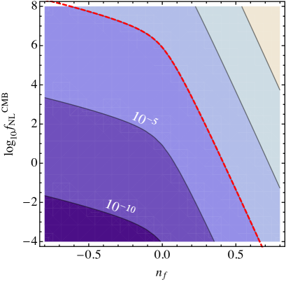
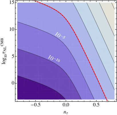
Figure 1: The constraints on $n_{f}$-$f^{\rm CMB}_{\rm NL}$ plane (left) and $n_{\tau}$-$\tau^{\rm CMB}_{\rm NL}$ plane (right). The interval of the contours of the $2C^{\Theta\Delta}_{50}/C^{\Theta\Theta}_{50}$(left) and $C^{\Delta\Delta}_{50}/C^{\Theta\Theta}_{50}$(right) are $10^{5}$, and red dashed lines correspond to the lines of $2C^{\Theta\Delta}_{50}=C^{\Delta\Delta}_{50}=C^{\Theta\Theta}_{50}$. Only the region below the red line is allowed.

In fig. 2, we show the constraints on the top hat type non-Gaussianities in the case with $n_{s}=1$. For simplicity, we also set $\widehat{\tau}_{\rm NL}=0$. Instead of giving the constraints on $\widetilde{f}_{\rm NL}$ and $\widetilde{\tau}_{\rm NL}$, we give the constraints directly on the magnitudes of bispectrum $B_{\mathcal{R}}=\widetilde{f}_{\rm NL}\mathcal{P}^{2}_{\mathcal{R}}(k_{0})$ and trispectrum $T_{\mathcal{R}}=\widetilde{\tau}_{\rm NL}\mathcal{P}^{3}_{\mathcal{R}}(k_{0})$. This is because $\widetilde{f}_{\rm NL}$ and $\widetilde{\tau}_{\rm NL}$ are normalized not by the (unknown) power spectrum at the corresponding scale but by that at the large (CMB) scale, that is, $P_{\mathcal{R}}(k_{0})$. The figure shows the constraints on bispectrum $B_{\mathcal{R}}$ and trispectrum $T_{\mathcal{R}}$. The contours of $(2C^{\Theta\Delta}_{50}+C^{\Delta\Delta}_{50})/C^{\Theta\Theta}_{50}$ are inserted at the interval of $10$ in the case with $\log_{10}k_{i}/k_{f}=4$, and a red dashed line corresponds to the line along which the non-linear correction is equal to $C^{\Theta\Theta}_{50}$. Then, only the region below the red line is allowed.

The disconnected part and the non-linear term proportional to $g_{\rm NL}$ do not contribute significantly. This is because such configurations do not pick up a pair of perturbations which are confined in the diffusion scale. The non-linear corrections to angular power spectra coming from these parts become

$$C^{\Delta\Delta,dc/g}_{l}= \frac{36\pi}{25}\int\frac{d^{3}k}{(2\pi)^{3}}j^{2}_{l}(k\eta_{0})P^{dc/g}_{\Delta}(k)$$

$$= \frac{36\pi}{25(2\pi^{2})}P^{dc/g}_{\Delta}(k\to 0)\int dkk^{2}j_{l}^{2}(k\eta_{0})\mathcal{W}_{r_{T}}(k).$$ (5.6)

Note that, in these cases, the use of the power spectra only for small $k$ modes is not justified because their spectra indexes are 4 and extremely blue, as already pointed out in (4.10) and (4.15). Therefore, we need to take into account the window function $\mathcal{W}_{r_{T}}$ or the exponential suppression factor $\exp{(-k^{2}/k_{D}^{2})}$ for large $k$ modes. Since $r_{T}\sim k_{D}(z_{5})^{-1}$, here, we simply take the Gaussian window function with $r_{T}$, $W_{r_{T}}(\mbox{\boldmath${x}$})=(1/(\sqrt{2\pi r_{T}})^{3})\exp(-r^{2}/(2r_{T}^{2}))$ and its Fourier component ${\cal W}_{r_{T}}(\mbox{\boldmath${k}$})=\exp(-r_{T}^{2}k^{2}/2)$, into account as a suppression factor for large $k$ modes, which enables us to integrate these expressions explicitly,

$$C^{\Delta\Delta,dc/g}_{l}= \frac{9}{25}\frac{1}{\sqrt{2\pi}\eta_{0}^{2}r_{T}}P^{dc/g}_{\Delta}(k\to 0)\left[1-\frac{r_{T}^{2}}{2\eta_{0}^{2}}l(l+1)+\mathcal{O}\left(\frac{r_{T}^{4}}{\eta_{0}^{4}}\right)\right]$$

$$\simeq 10^{-7}\frac{P^{dc/g}_{\Delta}(k\to 0)}{(2\pi^{2})},$$ (5.7)

where we have used

$$\int dkk^{2}j_{l}^{2}(k\eta_{0})\exp\left(-\frac{1}{2}r_{T}^{2}k^{2}\right)= \frac{\pi}{2}\frac{1}{\eta_{0}r_{T}^{2}}\exp\left(-\frac{\eta_{0}^{2}}{r_{T}^{2}}\right)I_{l+\frac{1}{2}}\left(\frac{\eta_{0}^{2}}{r_{T}^{2}}\right)$$

$$= \frac{\sqrt{\pi}}{2\sqrt{2}\eta_{0}^{2}r_{T}}\left[1-\frac{r_{T}^{2}}{2\eta_{0}^{2}}l(l+1)+\mathcal{O}\left(\frac{r^{4}_{T}}{\eta_{0}^{4}}\right)\right],$$ (5.8)

and the asymptotic expression for the modified Bessel function $I_{l+\frac{1}{2}}(z)$ given by

$$I_{l+\frac{1}{2}}(z)=\frac{e^{z}}{\sqrt{2\pi z}}\left[1-\frac{l(l+1)}{2z}+\mathcal{O}(z^{-2})\right].$$ (5.9)

Note that the spectral indexes are 4, which implies that the dimensionful power spectra $P^{dc/g}_{\Delta}(k\to 0)$ for small $k$ modes have no $k$ dependence. We have also substituted $r_{T}\simeq\mathcal{O}(0.1{\rm Mpc})$.

In passing, one also finds that (4.10) and (5.7) yield the weak constraints on power spectrum at $k\simeq k_{D}(z_{5})$

$$\mathcal{P}_{\mathcal{R}}(\mathcal{O}(10{\rm Mpc}^{-1}))\lesssim\mathcal{O}(0.1).$$ (5.10)

However, we have already known the stronger constraints on the scale by spectral distortions [7, 8, 9, 10, 11, 12, 13]. On the other hand, the constraints on $g_{\rm NL}$ can be about $10^{7}$ times weaker than those for $\tau_{\rm NL}$, comparing the cases with scale-independent local type $\tau_{\rm NL}$ and $g_{\rm NL}$.

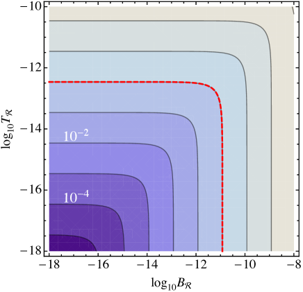
Figure 2: The figure shows the constraints on $B_{\mathcal{R}}=\widetilde{f}_{\rm NL}\mathcal{P}^{2}_{\mathcal{R}}(k_{0})$ and trispectrum $T_{\mathcal{R}}=\widetilde{\tau}_{\rm NL}\mathcal{P}^{3}_{\mathcal{R}}(k_{0})$. The contours of $(2C^{\Theta\Delta}_{50}+C^{\Delta\Delta}_{50})/C^{\Theta\Theta}_{50}$ are inserted at the interval of $10$ in the case with $\log_{10}k_{i}/k_{f}=4$, and a red dashed line is the line along which the non-linear correction is equal to $C^{\Theta\Theta}_{50}$. Only the region below the red line is allowed.

6 Conclusions and discussions

We have discussed the inhomogeneities of the acoustic reheating developing the previous works which have mainly focused on the homogeneous part. Such inhomogeneities arise from the higher order correlation functions of primordial curvature perturbations because the acoustic reheating is a non-linear phenomenon, which first appear at the second order in perturbation. Produced (secondary) temperature perturbations are, in general, indistinguishable from the standard temperature perturbations linearly coming from primordial curvature perturbations. Given the fact that the linear theory prediction well matches with the CMB observations, the non-linear corrections should be subdominant compared to the observational $C^{TT}_{l}$, i.e. the order of $10^{-10}$ at large scales. Based on this condition, we gave constraints on higher order correlation functions, especially, the scale dependent local type non-Gaussianities of primordial curvature perturbations, in which large- and small-scale perturbations are correlated. These configurations of bispectra of primordial curvature perturbations are complementary to those directly inferred from the three point correlation functions of the CMB anisotropies. Though the power spectra of the CMB anisotropies are used to constrain the (small-scale) higher order correlation functions of primordial curvature perturbations, the extension to the higher order correlation functions such as bispectrum and trispectrum of the CMB anisotropies to further constrain primordial curvature perturbations is straightforward.

In this paper, we have used only the total temperature perturbations to constrain the small-scale non-Gaussianities. However, the acoustic reheating can generate isocurvarture perturbations because the ratio of the number density of photon and baryon (dark matter, neutrino) is perturbed universally, as already pointed out in [19]. The constraint on isocurvature perturbations may give more stringent constraints on the small-scale primordial perturbations. This topic will be discussed elsewhere [39].

Appendix A Scale-dependent non-Gaussianity

In Fourier space, the bispectrum of the comoving curvature perturbation is written as

$$\langle\mathcal{R}_{\bm{k}_{1}}\mathcal{R}_{\bm{k}_{2}}\mathcal{R}_{\bm{k}_{3}}\rangle=(2\pi)^{3}\delta^{(3)}(\bm{k}_{1}+\bm{k}_{2}+\bm{k}_{3})B_{\mathcal{R}}(k_{1},k_{2},k_{3}),$$ (A.1)

and the local type one is parameterized as follows.

$$B_{\mathcal{R}}(k_{1},k_{2},k_{3})=-\frac{6}{5}f_{\rm NL}(k_{1},k_{2},k_{3})P^{2}_{\mathcal{R}}(k_{0})(x_{1}^{n_{s}-4}x_{2}^{n_{s}-4}+2{\rm perms.}),$$ (A.2)

where $x_{\alpha}=k_{\alpha}/k_{0}$. Now, let us consider scale-dependent local type non-Gaussianity defined as [36]

$$f^{G/A}_{\rm NL}(k_{1},k_{2},k_{3})=f^{\rm CMB}_{\rm NL}X_{G/A}^{n_{f}}$$ (A.3)

with $X_{G}=(x_{1}x_{2}x_{3})^{\frac{1}{3}}$ and $X_{A}=(x_{2}+x_{2}+x_{3})/3$. $f^{\rm CMB}_{\rm NL}$ is the $f_{\rm NL}$ parameter at the pivot scale $k_{0}$. In our cases, we can pick up the configuration of squeezed isosceles triangles, $k\ll k_{1}$, so we obtain the following forms.

$$f^{G}_{\rm NL}(k_{1},k_{1},k) =f^{\rm CMB}_{\rm NL}x_{1}^{\frac{2n_{f}}{3}}x^{\frac{n_{f}}{3}},$$ (A.4)

$$f^{A}_{\rm NL}(k_{1},k_{1},k) \simeq f^{\rm CMB}_{\rm NL}\left(\frac{2x_{1}}{3}\right)^{n_{f}}.$$ (A.5)

For the top hat type, using the top hat function defined as $W(x)=\theta(x-x_{i})-\theta(x-x_{f})$ with $\theta(x)$ being the step function, $f^{\rm tophat}_{\rm NL}(k_{1},k_{2},k_{3})$ can be written as

$$f^{\rm tophat}_{\rm NL}(k_{1},k_{2},k_{3})= f^{\rm CMB}_{\rm NL}+\widetilde{f}^{(1)}_{\rm NL}(W(x_{1})+2{\rm perms.})$$

$$+\widetilde{f}^{(2)}_{\rm NL}\left(W(x_{1})W(x_{2})+2{\rm perms}.\right)$$

$$+\widetilde{f}^{(3)}_{\rm NL}W(x_{1})W(x_{2})W(x_{3}).$$ (A.6)

Assuming that the squeezed isosceles triangle configurations are enhanced, that is $W(x)\simeq 0$, we can simplify (A.6) to

$$f^{\rm tophat}_{\rm NL}(k_{1},k_{1},k)=f^{\rm CMB}_{\rm NL}+\widetilde{f}_{\rm NL}W(x_{1}),$$ (A.7)

where $\widetilde{f}_{\rm NL}=2\widetilde{f}^{(1)}_{\rm NL}+\widetilde{f}^{(2)}_{\rm NL}$. The trispectrum is also introduced in the same manner with the bispectrum, and we do not repeat it here [37]. Assuming the power law type, the scale dependence can be written as

$$\tau_{\rm NL}(x_{1},x_{2},x^{\prime}_{1},x^{\prime}_{2})=\tau^{\rm CMB}_{\rm NL}Y^{n_{\tau}}_{G/A},$$ (A.8)

where we have defined $Y_{G}=(x_{1}x_{2}x_{3}x_{4})^{\frac{1}{4}}$ and $Y_{A}=(x_{1}+x_{2}+x_{3}+x_{4})/4$. For the geometric averaged type, the above formula can be reduced to

$$T^{G}_{\mathcal{R}}(k_{1},k_{1},k^{\prime}_{1},k^{\prime}_{1})=\tau^{\rm CMB}_{\rm NL}x_{1}^{n_{\tau}/2}{x^{\prime}_{1}}^{n_{\tau}/2}.$$ (A.9)

Top hat type is also defined as,

$$\tau^{\rm tophat}_{\rm NL}(x_{1},x_{1},x^{\prime}_{1},x^{\prime}_{1})=\tau^{\rm CMB}_{\rm NL}+\widehat{\tau}_{\rm NL}\left(W(x_{1})+W(x^{\prime}_{1})\right)+\widetilde{\tau}_{\rm NL}W(x_{1})W(x^{\prime}_{1}).$$ (A.10)

References

- [1] G. Hinshaw et al. [WMAP Collaboration], Astrophys. J. Suppl. 208, 19 (2013) [arXiv:1212.5226 [astro-ph.CO]].
- [2] P. A. R. Ade et al. [Planck Collaboration], arXiv:1502.02114 [astro-ph.CO].
- [3] E. Komatsu and D. N. Spergel, Phys. Rev. D 63 (2001) 063002 [astro-ph/0005036].
- [4] J. M. Maldacena, JHEP 0305, 013 (2003) [astro-ph/0210603].
- [5] Y. B. Zeldovich and R. A. Sunyaev, Astrophys. Space Sci. 4, 301 (1969).
- [6] R. A. Sunyaev and Y. B. Zeldovich, Astrophys. Space Sci. 7, 20 (1970).
- [7] W. Hu, D. Scott and J. Silk, Astrophys. J. 430, L5 (1994) [astro-ph/9402045].
- [8] J. D. Barrow & P. Coles, Mon. Not. Roy. Astron. Soc., 248, 52 (1991).
- [9] R. A. Daly, Astrophys. J. 371, 14 (1991).
- [10] J. Chluba, A. L. Erickcek and I. Ben-Dayan, Astrophys. J. 758, 76 (2012) [arXiv:1203.2681 [astro-ph.CO]].
- [11] R. Khatri, R. A. Sunyaev and J. Chluba, Astron. Astrophys. 543, A136 (2012) [arXiv:1205.2871 [astro-ph.CO]].
- [12] R. Khatri and R. A. Sunyaev, JCAP 1206, 038 (2012) [arXiv:1203.2601 [astro-ph.CO]].
- [13] J. Chluba, R. Khatri and R. A. Sunyaev, Mon. Not. Roy. Astron. Soc. 425, 1129 (2012) [arXiv:1202.0057 [astro-ph.CO]].
- [14] A. Kogut, D. J. Fixsen, D. T. Chuss, J. Dotson, E. Dwek, M. Halpern, G. F. Hinshaw and S. M. Meyer et al., JCAP 1107, 025 (2011) [arXiv:1105.2044 [astro-ph.CO]].
- [15] P. Andre et al. [PRISM Collaboration], arXiv:1306.2259 [astro-ph.CO].
- [16] J. C. Mather, E. S. Cheng, D. A. Cottingham, R. E. Eplee, D. J. Fixsen, T. Hewagama, R. B. Isaacman and K. A. Jesnsen et al., Astrophys. J. 420, 439 (1994).
- [17] D. J. Fixsen, E. S. Cheng, J. M. Gales, J. C. Mather, R. A. Shafer and E. L. Wright, Astrophys. J. 473, 576 (1996) [astro-ph/9605054].
- [18] R. Salvaterra and C. Burigana, Mon. Not. Roy. Astron. Soc. 336, 592 (2002) [astro-ph/0203294].
- [19] D. Jeong, J. Pradler, J. Chluba and M. Kamionkowski, Phys. Rev. Lett. 113, 061301 (2014) [arXiv:1403.3697 [astro-ph.CO]].
- [20] T. Nakama, T. Suyama and J. Yokoyama, Phys. Rev. Lett. 113, 061302 (2014) [arXiv:1403.5407 [astro-ph.CO]].
- [21] J. Chluba and R. A. Sunyaev, Astron. Astrophys. 424, 389 (2003) [astro-ph/0404067].
- [22] E. Pajer and M. Zaldarriaga, Phys. Rev. Lett. 109, 021302 (2012) [arXiv:1201.5375 [astro-ph.CO]].
- [23] Danese, L.; de Zotti, G. : Astronomy and Astrophysics, vol. 107, no. 1, Mar. 1982, p. 39-42. Research supported by the Consiglio Nazionale delle Ricerche.
- [24] J. Chluba, S. Y. Sazonov and R. A. Sunyaev, Astron. Astrophys. [Astron. Astrophys. 468, 785 (2007)] [astro-ph/0611172].
- [25] C. Burigana, L. Danese, and G. de Zotti, Astron. Astrophysics, 246, 49 (1991)
- [26] J. R. Bond and G. Efstathiou, Astrophys. J. 285, L45 (1984).
- [27] H. Kodama and M. Sasaki, Int. J. Mod. Phys. A 1 (1986) 265.
- [28] C. P. Ma and E. Bertschinger, Astrophys. J. 455, 7 (1995) [astro-ph/9506072].
- [29] A. Kosowsky, Annals Phys. 246, 49 (1996) [astro-ph/9501045].
- [30] W. Hu and N. Sugiyama, Astrophys. J. 471, 542 (1996) [astro-ph/9510117].
- [31] N. Bartolo, S. Matarrese and A. Riotto, JCAP 0606 (2006) 024 [astro-ph/0604416].
- [32] N. Bartolo, S. Matarrese and A. Riotto, JCAP 0701 (2007) 019 [astro-ph/0610110].
- [33] Z. Huang and F. Vernizzi, Phys. Rev. Lett. 110 (2013) 10, 101303 [arXiv:1212.3573 [astro-ph.CO]].
- [34] G. W. Pettinari, C. Fidler, R. Crittenden, K. Koyama and D. Wands, JCAP 1304 (2013) 003 [arXiv:1302.0832 [astro-ph.CO]].
- [35] Z. Huang and F. Vernizzi, Phys. Rev. D 89 (2014) 2, 021302 [arXiv:1311.6105 [astro-ph.CO]].
- [36] E. Sefusatti, M. Liguori, A. P. S. Yadav, M. G. Jackson and E. Pajer, JCAP 0912, 022 (2009) [arXiv:0906.0232 [astro-ph.CO]].
- [37] C. T. Byrnes, M. Sasaki and D. Wands, Phys. Rev. D 74, 123519 (2006) [astro-ph/0611075].
- [38] R. A. Sunyaev and Y. .B. Zeldovich, Astrophys. Space Sci. 9, 368 (1970).
- [39] A. Ota and M. Yamaguchi, in preparation.