A contact model for sticking of adhesive meso-particles

Abstract

The interaction between visco-elasto-plastic and adhesive particles is the subject of this study, where “meso-particles” are introduced, i.e., simplified particles, whose contact mechanics is not taken into account in all details. A few examples of meso-particles include agglomerates or groups of primary particles, or inhomogeneous particles with micro-structures of the scale of the contact deformation, such as core-shell materials.

A simple, flexible contact model for meso-particles is proposed, which allows to model the bulk behavior of assemblies of many particles in both rapid and slow, quasi-static flow situations. An attempt is made to categorize existing contact models for the normal force, discuss all the essential mechanical ingredients that must enter the model (qualitatively) and finally solve it analytically.

The model combines a short-ranged, non-contact part (resembling either dry or wet materials) with an elaborate, visco-elasto-plastic and adhesive contact law. Using energy conservation arguments, an analytical expression for the coefficient of restitution is derived in terms of the impact velocity (for pair interactions or, equivalently, without loss of generality, for quasi-static situations in terms of the maximum overlap or confining stress).

Adhesive particles (or meso-particles) stick to each other at very low impact velocity, while they rebound less dissipatively with increasing velocity, in agreement with previous studies. For even higher impact velocities an interesting second sticking and rebound regime is reported. The low velocity sticking is due to non-contact adhesive forces, the first rebound regime is due to stronger elastic and kinetic energies with little dissipation, while the high velocity sticking is generated by the non-linearly increasing, history dependent plastic dissipation and adhesive contact force. As the model allows also for a stiff, more elastic core material, this causes the second rebound regime at even higher velocities.

Keywords: Meso-scale particles and contact models, Particle collisions, Plastic loading-unloading cycles, Sticking, Adhesive contacts, Cohesive powders, Elasto-plastic material, Core-shell particles

Nomenclature

$m_{i}$	:	mass of $i^{th}$ particle.
$a_{i}$	:	Radius of $i^{th}$ particle.
$m_{r}$	:	Reduced mass of a pair of particles.
$\delta$	:	Contact overlap between particles.
$v_{i}$	:	Relative velocity before collision.
$v_{f}$	:	Relative velocity after collision.
${v_{i}}^{\infty}$	:	Relative velocity before collision at infinite separation.
${v_{f}}^{\infty}$	:	Relative velocity after collision at infinite separation.
$v^{n}$	:	Normal component of relative velocity.
$e$	:	Coefficient of restitution.
$e_{n}$	:	Normal coefficient of restitution.
$\epsilon_{i}$	:	Pull-in coefficient of restitution.
$\epsilon_{o}$	:	Pull-off coefficient of restitution.
$k$	:	Spring stiffness.
$k_{1}$	:	Slope of loading plastic branch.
$k_{2}$	:	Slope of unloading and re-loading elastic branch.
$k_{c}$	:	Slope of irreversible, tensile adhesive branch.
$k_{p}$	:	Slope of unloading and re-loading limit branch; end of plastic regime.
$v_{p}$	:	Relative velocity before collision for which the limit case is reached.
$\phi_{f}$	:	Dimensionless plasticity depth.
$\delta_{\rm max}$	:	Maximum overlap between particles during a collision.
$\delta^{p}_{\rm max}$	:	Maximum overlap between particles for the limit case.
$\delta_{\rm 0}$	:	Force free overlap $\cong$ plastic contact deformation.
$\delta_{\rm min}$	:	Overlap between particles at the maximum (negative) attractive force.
$\delta_{\rm c}$	:	Kinetic energy free overlap between particles.
$W_{\rm diss}$	:	Amount of energy dissipated during collision.
$\eta$	:	Dimensionless plasticity of the contact.
$\beta$	:	Adhesivity: dimensionless adhesive strength of the contact.
$\chi$	:	Scaled initial velocity relative to $v_{p}$.
$f_{a}$	:	Non-contact adhesive force at zero overlap.
$\delta_{\rm a}$	:	Non-contact separation between particles at which attractive force becomes active.
$k_{c}^{a}$	:	Strength of non-contact adhesive force.

1 Introduction

Granular materials and powders are ubiquitous in industry and nature. For this reason, the past decades have witnessed a strong interest in research aiming for better understanding and predicting their behavior in all regimes from flow to static as well as the transitions between these states. Especially, the impact of fine particles with other particles or surfaces is of fundamental importance. The interaction force between two particles is a combination of elasto-plastic deformation, viscous dissipation, and adhesion – due to both mechanical contact- and long ranged non-contact forces. Pair interactions that can be used in bulk simulations with many particles and multiple contacts per particle are the focus here, and we use the special, elementary case of pair interactions to understand them analytically.

Different regimes can be observed for collisions between two particles: For example, a particle can either stick to another particle/surface or it rebounds, depending upon the relative strength of adhesion and impact velocity, size and material various material parameters [1]. This problem needs to be well understood, as it forms the basis for understanding rather complex, many-particle flows in realistic systems, related to e.g. astrophysics (dust agglomeration, Saturn’s rings, planet formation) or industrial processes (handling of fine powders, granulation, filling and discharging of silos). Particularly interesting are the interaction mechanisms for adhesive materials such as asphalt, ice particles or clusters/agglomerates of fine powders (often made of even smaller primary particles). Some of these materials can be physically visualized as having a plastic outer shell with a stronger and more elastic inner core. Understanding this can then be applied to particle-surface collisions in kinetic spraying, where the solid micro-sized powder particle is accelerated towards a substrate. In cold spray, bonding occurs when impact velocities of particles exceed a critical value, which depends on various material parameters [2, 3, 4, 1]. However, for even higher velocities particles rebound from the surface [5, 6]. Due to the inhomogeneity of most realistic materials, their non-sphericity and their surface irregularity, one can not include all these details – but rather has to focus on the essential phenomena and ingredients, finding a compromise between simplicity and realistic contact mechanics.

1.1 Contact Models Review

Computer simulations have turned out to be a powerful tool to investigate the physics of particulate systems, especially valuable as experimental difficulties are considerable and since there is no generally accepted theory of granular flows. A very popular simulation scheme is an adaptation of the classical Molecular Dynamics technique called Discrete Element Method (DEM) (for details see Refs. [7, 8, 9, 10, 11, 12, 13, 14, 15]). It involves integrating Newton’s equations of motion for a system of “soft”, deformable grains, starting from a given initial configuration. DEM can be successfully applied to adhesive particles, if a proper force-overlap law (contact model) is used.

The JKR model [16] is a widely accepted contact model for adhesive elastic spheres and gives an expression for the normal force in terms of the normal deformation. Derjaguin et al. [17] suggested that the attractive forces act only just outside the contact zone, where surface separation is small, and is referred to as DMT model. An interesting approach for dry adhesive particles was proposed by Molerus [18, 19], who explained consolidation and non-rapid flow of adhesive particles in terms of adhesive forces at particle contacts. Thornton and Yin [20] compared the results of elastic spheres with and without adhesion, a work that was later extended to adhesive elasto-plastic spheres [21]. Molerus’s model was further developed by Tomas, who introduced a complex contact model [22, 23, 24] by coupling elasto-plastic contact behavior with non-linear adhesion and hysteresis involving dissipation and a history (compression) dependent adhesive force. The contact model subsequently proposed by Luding [25, 15] works in the same spirit as that of Tomas [23], only reducing complexity by using piece-wise linear branches in an otherwise non-linear contact model in spirit (as explained later in this study). In the original version [15], a short-ranged force beyond contact was mentioned, but not specified, which is one of the issues tackled in the present study. Contact details, such as a possible non-linear Hertzian law for small deformation, and non-linear loading-unloading hysteresis are over-simplified in Ludings model, as compared to the model proposed by Tomas [23]. This is partly due to the lack of the experimental reference data or theories, but also motivated by the wish to keep the model as simple as possible. The model consists of several basic mechanisms, i.e., non-linear elasticity, plasticity and adhesion as relevant for, e.g. core-shell materials or agglomerates of fine, dry primary powder particles [26, 27]. A possible connection between the microscopic contact model and the macroscopic, continuum description for adhesive particles was recently proposed by Luding et al. [28], as further explored by Singh et al. [29, 30] for dry adhesion, by studying the force anisotropy and force distributions in steady state bulk shear in the , which is further generalized to wet adhesion by Roy et al. [33], or studied under shear-reversal [34, 35].

Jiang et al. [36] experimentally investigated the force-displacement behavior of idealized bonded granules. This was later used to study the mechanical behavior of loose cemented granular materials using DEM simulations [37]. Kempton et al. [38] proposed a meso-scale contact model combining linear hysteretic, simplified JKR and linear bonding force models, to simulate agglomerates of sub-particles. The phenomenology of such particles is nicely described by Dominik and Tielens [26]. Walton et al. [39, 40] also proposed contact models in similar spirit as that of Luding [15] and Tomas [23], separating the pull-off force from the slope of the tensile attractive force as independent mechanisms. Most recently two contact models were proposed by Thakur et al. [41] and by Pasha et al. [42], which work in the same spirit as Luding’s model, but treat loading and un/re-loading behaviors differently. The former excludes the non-linear elastic stiffness in the plastic regime, and both deal with a more brittle, abrupt reduction of the adhesive contact force. The authors further used their models to study the scaling and effect of DEM parameters in an uniaxial compression test [43], and compared part of their results with other models [42].

When two particles interact, their behavior is intermediate between the extremes of perfectly elastic and fully inelastic, possibly even fragmenting, where the latter is not considered in this study. Considering a dynamic collision is our choice here, but without loss of generality, most of our results can also be applied to a slow, quasi-static loading-unloading cycle that activates the plastic loss of energy, by replacing kinetic with potential energies. Rozenblat et al.  [44] have recently proposed an empirical relation between impact velocity and static compression force.

The amount of energy dissipated during a collision can be best quantified by the coefficient of restitution, which is the ratio of magnitude of post-collision and pre-collision normal relative velocities of the particles. It quantifies the amount of energy that is not dissipated during the collision. For the case of plastic and viscoelastic collisions, it was suggested that dissipation depends on impact velocity [45, 46, 47]; this can be realized by viscoelastic forces [46, 48, 49, 50] and follows from plastic deformations too [51].

Early experimental studies [52, 53] on adhesive polystyrene latex spheres of micrometer size showed sticking of particles for velocities below a threshold and an increasing coefficient of restitution for velocities increasing above the threshold. Wall et al. [54] further confirmed these findings for highly mono-disperse ammonium particles. Thornton et al. [21] and Brilliantov et al. [55] proposed an adhesive visco-elasto-plastic contact model in agreement with these experiments. Work by Sorace et al. [56] also confirms the sticking at low velocities for particle sizes of the order of a few mm. Li et al. [57] proposed a dynamical model based on JKR for the impact of micro-sized spheres with a flat surface, whereas realisitc particle contacts are usually not flat [58]. Recently, Saitoh et al. [59] even reported negative coefficients of restitution in nanocluster simulations, which is an artefact of the wrong definition of the coefficient of restitution; one has to relate the relative velocities to the normal directions before and after collision and not just in the frame before collision, which is especially a serious effect for softer particles [60]. Jasevic̆ius et al. [61, 62] have recently studied the rebound behavior of ultrafine silica particles using the contact model by Tomas [22, 23, 24, 63]. They found that energy absorption due to attractive forces is the main source of energy dissipation at lower impact velocities or compression, while plastic deformation-induced dissipation becomes more important with increasing impact velocity. They found some discrepancies between numerical and experimental observations and concluded that these might be due to the lack of knowledge of particle- and contact-parameters, including surface roughness, adsorption layers on particle surfaces, and microscopic material property distributions (inhomogeneities), which in essence are features of the meso-particles that we aim to study.

In a more recent study, Shinbrot et al. [64] studied charged primary particles with interesting single particle dynamics in the electromagnetic field. They found ensembles of attractive (charged) particles can forming collective contacts or even fingers, extending the concepts of “contact” well beyond the idealized picture of perfect spheres, as shown also in the appendix of the present study.

Finally, Rathbone et al. [65] presented a new force-displacement law for elasto-plastic materials and compare it to their FEM results that resolve the deformations in the particle contact zone. This was complemented by an experimental study comparing various models and their influence on the bulk flow behavior [1].

1.2 Model classification

Since our main focus is on dry particles, here we do not review the diverse works that involve liquid [66] or strong solid bridges [67]. Even though oblique collisions between two particles are of practical relevance and have been studied in detail by Thornton et al. [68, 69], here we focus on central normal collisions without loss of generality. Finally, we also disregard many minute details of non-contact forces, as, e.g. due to van der Waals forces, for the sake of brevity, but will propose a very simple mesoscale non-contact force model in section 2.3.

Based on our review of adhesive, elasto-visco-plastic contact models, here we propose a possible classification, by dividing them into three groups (based on their complexity and aim):
(1) Academic contact models,
(2) Mesoscopic contact models, and
(3) Realistic, fully detailed contact models.
Here we focus on adhesive elastic, and elasto-plastic contact models mainly, while the effect of various forces on adhesion of fine particles is reviewed in Ref. [70], and some of the more complex models are reviewed and compared in Ref. [69].

1. Academic contact models allow for easy analytical solution, as for example the linear spring-dashpot model [50], or piece-wise linear models with constant unloading stiffness (see e.g. Walton and Braun [71]), which feature a constant coefficient of restitution (independent of impact velocity). Also the Hertzian visco-elastic models belong to this class, even though they provide a velocity dependent coefficient of restitution, for a summary see Ref. [50] and references therein, while for a recent comparison see Ref. [72]. However, no academic model can fully describe realistic, practically relevant contacts. Either the material or the geometry/mechanics is too idealized; in application, there is hardly any contact that is perfectly linear or Hertzian visco-elastic. Academic models thus miss most details of real contacts, but can be treated analytically.

2. Mesoscopic contact models (or, with other words, contact models for meso-particles) are a compromise, (i) still rather easy to implement, (ii) aimed for fast ensemble/bulk-simulations with many particles and various materials, and (iii) contain most relevant mechanisms, but not all the minute details of every primary particle and every single contact. They are often piece-wise linear, e.g. with a variable unloading stiffness or with an extended adhesive force, leading to a variable coefficient of restitution, etc., see Refs. [71, 15, 40, 73, 41]).

3. Realistic, full-detail contact models have (i) the most realistic, but often rather complicated formulation, (ii) can reproduce with similar precision the pair interaction and the bulk behavior, but (iii) are valid only for the limited class of materials they are particularly designed for, since they do include all the minute details of these interactions. A few examples include:

   1. visco-elastic models: Walton [74], Brilliantov [75, 55], Haiat [76];

   2. adhesive elastic models: JKR [16], Dahneke [77], DMT [17], Thornton and Yin [20];

   3. adhesive elasto-plastic models: Molerus[18], Thornton and Ning [21], Tomas [22, 23, 24, 63], Pasha et al. [42].

While the realistic models are designed for a special particulate material in mind, our main goal is to define and apply mesoscopic contact models to simulate the bulk behavior of a variety of assemblies of many particles (for which no valid realistic model is available), we focus on the second class: mesoscopic contact models.

1.3 Focus and Overview of this study

In particular, we study the dependence of the coefficient of restitution for two meso-particles on impact velocity and contact/material parameters, for a wide range of impact velocities, using the complete version of the contact model by Luding [15], with a specific piece-wise linear non-contact force term. We observe sticking of particles at low velocity, which is consistent with previous theoretical and experimental works [54, 21, 56]. Pasha et al. [42] recently also reproduced the low velocity sticking using an extension of the similar, but simpler model [78]. Above a certain small velocity, dissipation is not strong enough to dissipate all relative kinetic energy and the coefficient of restitution begins to increase. We want to understand the full regime of relative velocities, and thus focus also on the less explored intermediate and high velocity regimes, as easily accessible in numerical simulations. In the intermediate regime, we observe a decrease in the coefficient of restitution, as observed previously for idealized/homogeneous particles [21, 55], however the functional behavior is different compared to the predictions by Thornton [21]. In Appendix 2.2.4, we show that this property can be tuned by simple modifications to our model. Tanaka et al. [79] have recently reported similar results, when simulating the collision of more realistic dust aggregates, consisting of many thousands of nanoparticles that interact via the JKR model. With further increase in impact velocity, we find a second sticking regime due to the non-linearly increasing adhesive and plastic dissipation. For even higher velocities, the second, intermediate sticking regime is terminated by a second rebound regime due to the elastic core that can be specified in the model. Finally, since the physical systems under consideration also are viscous in nature, we conclude with some simulations with added viscous damping, which is always added on top of the other model ingredients, but sometimes neglected in order to allow for analytical solutions.

An exemplary application of our model that shows the unexpected high velocity sticking and rebound regime (which might not be observed in the case of homogeneous granular materials) is, the coating process in cold sprays. In these studies, the researchers are interested in analyzing the deposition efficiency of the powder on a substrate as a function of the impact velocity. Bonding/coating happens when the impact velocity of the particles exceeds a “critical velocity”, with values of the order of $10^{2}$ m/s [4, 5, 6]. Interestingly, when the velocity is further increased the particles do not bond (stick) to the substrate anymore, and a decrease in the deposition efficiency (inverse of the coefficient of restitution) is observed [5]. Schmidt et al. [4] have used numerical simulations to explore the effect of various material properties on the critical velocity, while Zhou et al. [6] studied the effect of impact velocity and material properties on the coating process, showing that properties of both particle and substrate influence the rebound. Using our model, one could explore the dependence of the deposition efficiency on the impact velocity, leading to the synergy between different communities.

The paper is arranged as follows: In section 2, we introduce the DEM simulation method and the basic contact models for the normal direction; one type of meso-models is further elaborated on in the following section 3, where the coefficient of restitution is computed analytically, and dimensionless contact parameters are proposed in section 4. The limit of negligible non-contact forces is considered in section 5, where various special cases are discussed, the contact model parameters are studied, and also asymptotic solutions and limit values are given, before the study is concluded in section 6.

2 Discrete Element Method

The elementary units of particulate systems as granular materials or powders are grains that deform under applied stress. Since the realistic and detailed modeling of real particles in contact is too complicated, it is necessary to relate the interaction force to the overlap $\delta$ between two particles in contact. Note that the evaluation of the inter-particle forces based on the overlap may not be sufficient to account for the inhomogeneous stress distribution inside the particles, for internal re-arrangements [26], and for possible multi-contact effects [45]. However, this price has to be paid in order to simulate large samples of particles with a minimal complexity and still taking various physical contact properties such as non-linear contact elasticity, plastic deformation or load-dependent adhesion into account.

2.1 Equations of Motion

If all forces acting on a spherical particle $p$, either from other particles, from boundaries or externally, are known – let their vector sum be $\vec{f}_{p}$ – then the problem is reduced to the integration of Newton’s equations of motion for the translational degrees of freedom (the rotational degrees are not considered here since we focus only on normal forces) for each particle: $m_{p}\frac{{\rm d}^{2}}{{\rm d}t^{2}}\vec{r_{p}}=\vec{f}_{p}+m_{p}\vec{g}$ where, $m_{p}$ is the mass of particle $p$, $\vec{r}_{p}$ its position, $\vec{f}_{p}=\sum_{c}\vec{f}^{c}_{p}$ is the total force due to all contacts $c$, and $\vec{g}$ is the acceleration due to volume forces like gravity. With tools as nicely described in textbooks as [80, 81, 82], the integration over many time-steps is a straightforward exercise. The typically short-ranged interactions in granular media allow for further optimization by using linked-cell (LC) or alternative methods in order to make the neighborhood search more efficient [83, 84]. However, such optimization issues are not of concern in this study, since only normal pair collisions are considered.

2.2 Normal Contact Force Laws

Two spherical particles $i$ and $j$, with radii $a_{i}$ and $a_{j}$, $r_{i}$ and $r_{j}$ being the position vectors respectively, interact if their overlap,

$$\delta=(a_{i}+a_{j})-(\vec{r}_{i}-\vec{r}_{j})\cdot\vec{n}~{},$$ (1)

is either positive, $\delta>0$, for mechanical contact, or smaller than a cut-off, $0\geq\delta>\delta_{a}$, for non-contact interactions, with the unit vector $\vec{n}=\vec{n}_{ij}=(\vec{r}_{i}-\vec{r}_{j})/|\vec{r}_{i}-\vec{r}_{j}|$ pointing from $j$ to $i$. The force on particle $i$, from particle $j$, at contact $c$, can be decomposed into a normal and a tangential part as $\vec{f}^{c}:=\vec{f}^{c}_{i}=f^{n}\vec{n}+f^{t}\vec{t}$, where $\vec{n}\cdot\vec{t}=0$, $n$ and $t$ being normal and tangential parts respectively. In this paper, we focus on frictionless particles, i.e., only normal forces will be considered, for tangential forces and torques, see e.g. Ref. [15] and references therein.

In the following, we discuss various normal contact force models, as shown schematically in Fig. 1. We start with the linear contact model (Fig. 1(a)) for non-adhesive particles, before we introduce a more complex contact model that is able to describe the realistic interaction between adhesive, inhomogeneous , slightly non-spherical particles (Fig. 1(b)).

 

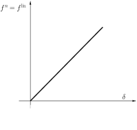
Figure 1: Schematic plots of contact forces for (a) the linear normal model for a perfectly elastic collision, and (b) the force-overlap relation for an elasto-plastic adhesive collision

2.2.1 Linear Normal Contact Model

Modelling a force that leads to an inelastic collision requires at least two ingredients: repulsion and some sort of dissipation. The simplest (but academic) normal force law with the desired properties is the damped harmonic oscillator

$$f^{n}=k\delta+\gamma_{0}v^{n}~{},$$ (2)

with spring stiffness $k$, viscous damping $\gamma_{0}$, and normal relative velocity $v^{n}=-{\vec{v}}_{ij}\cdot{\vec{n}}=-(\vec{v}_{i}-\vec{v}_{j})\cdot\vec{n}=\dot{\delta}$. This model (also called linear spring dashpot (LSD) model) has the advantage that its analytical solution (with initial conditions $\delta(0)=0$ and $\dot{\delta}(0)=v^{n}_{0}$) allows easy calculations of important quantities [50]. For the non-viscous case, the linear normal contact model is given schematically in Fig. 1.

The typical response time (contact duration) and the eigenfrequency of the contact are related as

$$t_{c}={\frac{\pi}{\omega}}~{}{\rm~{}~{}~{}and~{}~{}~{}}\omega=\sqrt{({k}/{m_{r}})-\eta_{0}^{2}}~{}$$ (3)

with the rescaled damping coefficient $\eta_{0}=\gamma_{0}/(2m_{r})$, and the reduced mass $m_{r}=m_{i}m_{j}/(m_{i}+m_{j})$, where the $\eta_{0}$ is defined such that it has the same units as $\omega$, i.e., frequency. From the solution of the equation of a half-period of the oscillation, one also obtains the coefficient of restitution

$$e^{\rm LSD}_{n}=v_{f}/v_{i}=\exp\left(-\pi\eta_{0}/\omega\right)=\exp\left(-\eta_{0}t_{c}\right)~{},$$ (4)

which quantifies the ratio of normal relative velocities after ($v_{f}$) and before ($v_{i}$) the collision. Note that in this model $e_{n}$ is independent of $v_{i}$. For a more detailed review on this and other, more realistic, non-linear contact models, see [50, 15] and references therein.

The contact duration in Eq. (3) is also of practical and technical importance, since the integration of the equations of motion is stable only if the integration time-step $\Delta t$ is much smaller than $t_{c}$. Note that $t_{c}$ depends on the magnitude of dissipation: In the extreme case of an over-damped spring (high dissipation), $t_{c}$ can become very large (which renders the contact behavior artificial [48]). Therefore, the use of neither too weak nor too strong viscous dissipation is recommended, so that some artificial effects are not observed by the use of viscous damping.

2.2.2 Adhesive Elasto-Plastic Contacts

Figure 2: Schematic graph of the piece-wise linear, hysteretic, and adhesive force-displacement model in normal direction from Ref. [15].

For completeness, we re-introduce the piece-wise linear hysteretic model [15] as an alternative to non-linear spring-dashpot models or more complex hysteretic models [22, 23, 24, 21, 85, 86]. It reflects permanent plastic deformation , which takes place at the contact, and the non-linear increase of both elastic stiffness and attractive (adhesive) forces with the maximal compression force.

In Fig. 2, the normal force at contact is plotted against the overlap $\delta$ between two particles. The force law can be written as

$$f^{\rm hys}=\left\{\begin{array}[]{lll}k_{1}\delta&&{\rm if~{}~{}}k_{2}(\delta-\delta_{0})\geq k_{1}\delta\\ k_{2}(\delta-\delta_{0})&&{\rm if~{}~{}}k_{1}\delta>k_{2}(\delta-\delta_{0})>-k_{c}\delta\\ -k_{c}\delta&&{\rm if~{}~{}}-k_{c}\delta\geq k_{2}(\delta-\delta_{0})\end{array}\right.$$ (5)

with $k_{1}\leq k_{2}\leq k_{p}$, respectively the initial loading stiffness, the un-/re-loading stiffness and the elastic limit stiffness. The latter defines the limit force branch $k_{p}(\delta-\delta^{p}_{0})$, as will be motivated next in more detail, and $k_{2}$ interpolates between $k_{1}$ and $k_{p}$, see Eq. (9). For $k_{c}=0$, the above contact model reduces to that proposed by Walton and Braun [71], with coefficient of restitution

$$e^{\rm WB}_{n}=\sqrt{k_{1}/k_{2}}~{}.$$ (6)

During the initial loading the force increases linearly with overlap $\delta$ along $k_{1}$, until the maximum overlap $\delta_{\rm max}=v_{i}\sqrt{{m_{r}}/{k_{1}}}$ (for binary collisions) is reached, which is a history parameter for each contact. During unloading the force decreases along $k_{2}$, see Eq. (9), from its maximum value $k_{1}\delta_{\rm max}$ at $\delta_{\rm max}$ down to zero at overlap

$$\delta_{0}=(1-k_{1}/k_{2})\delta_{\rm max}~{},$$ (7)

where $\delta_{0}$ resembles the permanent plastic contact deformation. Re-loading at any instant leads to an increase of the force along the (elastic) branch with slope $k_{2}$, until the maximum overlap $\delta_{\rm max}$ (which was stored in memory) is reached; for still increasing overlap $\delta$, the force again increases with slope $k_{1}$ and the history parameter $\delta_{\rm max}$ has to be updated.

Unloading below $\delta_{0}$ leads to a negative, attractive (adhesive) force, which follows the line with slope $k_{2}$, until the extreme adhesive force $-k_{c}\delta_{\rm min}$ is reached. The corresponding overlap is

$$\delta_{\rm min}=\frac{({k_{2}-k_{1}})}{({k_{2}+k_{c}})}\delta_{\rm max}~{}.$$ (8)

Further unloading follows the irreversible tensile limit branch, with slope $-k_{c}$, with the attractive force $f^{\rm hys}=-k_{c}\delta$.

The lines with slope $k_{1}$ and $-k_{c}$ define the range of possible positive and negative forces. Between these two extremes, unloading and/or re-loading follow the line with slope $k_{2}$. A non-linear un-/re-loading behavior would be more realistic, however, due to a lack of detailed experimental informations, the piece-wise linear model is used as a compromise, besides that it is easier to implement. The elastic $k_{2}$ branch becomes non-linear and ellipsoidal if a moderate normal viscous damping force is active at the contact, as in the LSD model.

In order to account for realistic load-dependent contact behavior, the $k_{2}$ value is chosen to depend on the maximum overlap $\delta_{\rm max}$, i.e. contacts are stiffer and more strongly plastically deformed for larger previous deformations so that the dissipation depends on the previous deformation history. The dependence of $k_{2}$ on overlap $\delta_{\rm max}$ is chosen empirically as linear interpolation:

$$k_{2}(\delta_{\rm max})=\left\{\begin{array}[]{lll}k_{p}\,{\rm~{}~{}~{}~{}~{}~{}~{}~{}~{}~{}~{}~{}~{}~{}~{}~{}~{}~{}~{}~{}~{}~{}~{}~{}if~{}~{}}\delta_{\rm max}/\delta^{p}_{\rm max}\geq 1\\ k_{1}+(k_{p}-k_{1}){\delta_{\rm max}}/{\delta^{p}_{\rm max}}&\\ ~{}~{}~{}~{}~{}~{}~{}~{}~{}~{}{\rm~{}~{}~{}~{}~{}~{}~{}~{}~{}~{}~{}~{}~{}~{}~{}~{}~{}~{}~{}if~{}~{}}\delta_{\rm max}/\delta^{p}_{\rm max}<1\end{array}\right.$$ (9)

where $k_{p}$ is the maximal (elastic) stiffness, and

$$\delta^{p}_{\rm max}=\frac{k_{p}}{k_{p}-k_{1}}\phi_{f}\frac{2{a_{1}a_{2}}}{a_{1}+a_{2}}~{},$$ (10)

is the plastic flow limit overlap, with $\phi_{f}$ the dimensionless plasticity depth, $a_{1}$ and $a_{2}$ being the radii of the two particles. This can be further simplified to

$$\delta^{p}_{0}=\phi_{f}a_{12},$$ (11)

where $\delta^{p}_{0}$ represents the plastic contact deformation at the limit overlap, and $a_{12}=\frac{2{a_{1}a_{2}}}{a_{1}+a_{2}}$ is the reduced radius. In the range $\delta_{\rm max}<\delta^{p}_{\rm max}$, the stiffness $k_{2}$ can also be written as:

$$k_{2}=k_{1}+\frac{(k_{p}-k_{1})}{k_{1}\delta^{p}_{\rm max}}f^{\rm max},$$ (12)

where $f^{\rm max}=k_{1}\delta_{\rm max}$ is the same as Eq. (4) in [71] with prefactor $S=\frac{(k_{p}-k_{1})}{k_{1}\delta^{p}_{\rm max}}$.

From energy balance considerations, one can define the “plastic” limit velocity

$$v_{p}=\sqrt{k_{1}/m_{r}}\,\delta^{p}_{\rm max}~{},$$ (13)

below which the contact behavior is elasto-plastic, and above which the perfectly elastic limit-branch is reached. Impact velocities larger than $v_{p}$ have consequences, as discussed next (see Sec. 2.2.4).

In summary, the adhesive, elasto-plastic, hysteretic normal contact model is defined by the four parameters $k_{1}$, $k_{p}$, $k_{c}$ and $\phi_{f}$ that, respectively, account for the initial plastic loading stiffness, the maximal, plastic limit (elastic) stiffness, the adhesion strength, and the plastic overlap-range of the model. This involves an empirical choice for the load-dependent, intermediate elastic branch stiffness $k_{2}$, which renders the model non-linear in its behavior (i.e. higher confinging stress leads to stiffer contacts like in the Hertz model), even though the present model is piece-wise linear.

2.2.3 Motivation of the original contact model

To study a collision between two ideal, homogeneous spheres, one should refer to realistic, full-detail contact models with a solid experimental and theoretical foundation [16, 21, 22]. These contact models feature a small elastic regime and the particles increasingly deform plastically with increasing, not too large deformation (overlap). During unloading, their contacts end at finite overlap due to flattening. An alternative model was recently proposed, see Ref. [42], that follows the philosophy of plastically flattened contacts with instantaneous detachment at positive overlaps.

However, one has to also consider the possibility of rougher contacts [58], and possible non-contact forces that are usually neglected for very large particles, but can become dominant and hysteretic as well as long-ranged for rather small spheres [26, 22].

The mesoscopic contact model used here, as originally developed for sintering [25], and later defined in a temperature-independent form [15], follows a different approach in two respects: (i) it introduces a limit to the plastic deformation of the particles/material for various reasons as summarized below and also in subsection 2.2.4, and (ii) the contacts are not idealized as perfectly flat, and thus do not have to lose mechanical contact immediately at un-loading, as will be detailed in subsection 2.2.5.

Note that a limit to the slope $k_{p}$ resembles a simplification of different contact behavior at large deformations:
(i) for low compression, due to the wide probability distribution of forces in bulk granular matter, only few contacts should reach the limit, which would not affect much the collective, bulk behavior;
(ii) for strong compression, in many particle systems, i.e., for large deformations, the particles cannot be assumed to be spherical anymore, and they deform plastically or could even break;
(iii) from the macroscopic point of view, too large deformations would lead to volume fractions larger than unity, which for most materials (except highly micro-porous, fractal ones) would be unaccountable;
(iv) at small deformation, contacts are due to surface roughness realized by multiple surface asperities and at large deformation, the single pair point-contact argument breaks down and multiple contacts of a single particle can not be assumed to be independent anymore;
(v) finally, (larger) meso-particles have a lower stiffness than (smaller) primary particles [41], which is also numerically relevant, since the time step has to be chosen such that it is well below the minimal contact duration of all the contacts. If $k_{2}$ is not limited the time-step could become prohibitively small, only because of a few extreme (large compression) contact situations.
The following two subsections discuss the two major differences of the present piece-wise linear (yet non-linear) model as compared to other existing models: (i) the elastic limit branch, and (ii) the elastic re-loading or non-contact-loss, as well as their reasons, relevance and possible changes/tuning – in case needed.

2.2.4 Shortcomings, physical relevance and possible tuning

In the context of collisions between perfect homogeneous elasto-plastic spheres, a purely elastic threshold/limit and enduring elastic behavior after a sharply defined contact-loss are indeed questionable, as the plastic deformation of the single particle cannot become reversible/elastic. Nevertheless, there are many materials that support the idea of a more elastic behavior at large compression (due to either very high impact velocity or multiple strong contact forces), as discussed further in the paragraphs below.

Mesoscopic contact model applied to real materials:

First we want to recall that the present model is mainly aimed to reproduce the behavior of multi-particle systems of realistic fine and ultra-fine powders, which are typically non-spherical and often mesoscopic in size with internal micro-structure and micro-porosity on the scale of typical contact deformation. For example, think of clusters/agglomerates of primary nano-particles that form fine micron-sized secondary powder particles, or other fluffy materials [26]. The primary particles are possibly better described by other contact models, but in order to simulate a reasonable number of secondary (meso) particles one cannot rely on this bottom-up approach and hence a mesoscopic contact model needs to be used. During the bulk compression of such a system, the material deforms plastically and both the bulk and particles’ internal porosity reduces [26]. Plastic deformation diminishes if the material becomes so dense, with minimal porosity, such that the elastic/stiff primary particles dominate. Beyond this point the system deforms more elastically, i.e. the stiffness becomes high and the (irrecoverable) plastic deformations are much smaller than at weaker compression.

In their compression experiments of granular beds with micrometer sized granules of micro-crystalline cellulose, Persson et al. [87] found that a contact model where a limit on plastic deformation is introduced can very well describe the bulk behavior. Experimentally they observe a strong elasto-plastic bulk-behavior for the assembly at low compression strain/stress. In this phase the height of the bed decreases, irreversibly with the applied load. It becomes strongly non-linear beyond a certain strain/stress, which is accompanied by a dramatic increase of the stiffness of the aggregate. They associate this change in the behavior to the loss of porosity and the subsequent more elastic bulk response to the particles that are now closely in touch with each other. In this new, re-structured, very compacted configurations, further void reduction is not allowed anymore and thus the behavior gets more elastic. While the elastic limit in the contact model does not affect the description of the bulk behavior in the first part, the threshold is found to play a key role in order to reproduce the material stiffening (see Fig. 8 in Ref. [87]).

Note that in an assembly of particles, not all the contacts will reach the limit branch and deform elastically simultaneously. That is, even if few contacts are in the elastic limit, the system will always retain some plasticity, hence the assembly will never be fully elastic.

Application to pair interactions:

Interestingly, the contact model in Sec. 2.2.2 is suitable to describe the collision between pairs of particles, when special classes of materials are considered, such that the behavior at high velocity and thus large deformation drastically changes.

(i) Core-shell materials. The model is perfectly suited for plastic core-shell materials, such as asphalt or ice particles, having a “soft” plastic outer shell and a rather stiff, elastic inner core. For such materials the stiffness increases with the load due to an increasing contact surface. For higher deformations, the inner cores can come in contact, which turns out to be almost elastic when compared to the behavior of the external shell. The model was successfully applied to model asphalt, where the elastic inner core is surrounded by a plastic oil or bitumen layer [88]. Alternatively, the plastic shell can be seen as the range of overlaps, where the surface roughness and inhomogeneities lead to a different contact mechanics as for the more homogeneous inner core.

(ii) Cold spray. An other interesting system that can be effectively reproduced by introducing an elastic limit in the contact model is cold spray. Researchers have experimentally and numerically shown that spray-particles rebound from the substrate at low velocities, while they stick at intermediate impact energy [2, 3, 4, 89]. Wu et al. [5] experimentally found that rebound re-appears with a further increase in velocity (Fig. 3 in Ref. [5]). Schmidt et al. [4] relate the decrease of the deposition efficiency (inverse of coefficient of restitution) to a transition from a plastic impact to hydrodynamic penetration (Fig. 16 in Ref. [4]). Recently, Moridi et al. [89] numerically studied the sticking and rebound processes, by using the adhesive elasto-plastic contact model of Luding [15], and their prediction of the velocity dependent behavior is in good agreement with experiments.

(iii) Sintering. As an additional example, we want to recall that the present mesoscopic contact model has already been applied to the case of sintering, see Ref. [25, 90]. For large deformations, large stresses, or high temperatures, the material goes to a fluid-like state rather than being solid. Hence, the elasticity of the system (nearly incompressible melt) determines its limit stiffness, while $\phi_{f}$ determines the maximal volume fraction that can be reached.

All the realistic situations described above clearly hint at a modification in the contact phenomenology that can not be described solely by an elasto-plastic model beyond some threshold in the overlap/force. The limit stiffness $k_{p}$ and the plastic layer depth $\phi_{f}$ in our model allow the transition of the material to a new state. Dissipation on the limit branch – which otherwise would be perfectly elastic – can be taken care of, by adding a viscous damping force (as the simplest option). Due to viscous damping, the unloading and re-loading will follow different paths, so that the collision will never be perfectly elastic, which is in agreement with the description in Jasevic̆ius et al. [61, 62] and will be shown later in Appendix B.

Finally, note that an elastic limit branch is surely not the ultimate solution, but a simple first model attempt – possibly requiring material- and problem-adapted improvements in the future.

Tuning of the contact model:

The change in behavior at large contact deformations is thus a feature of the contact model which allows us to describe many special types of materials. Nevertheless, if desired (without changing the model), the parameters can be tuned in order to reproduce the behavior of materials where the plasticity increases with deformation without limits, i.e., the elastic core feature can be removed. The limit-branch where plastic deformation ends is defined by the dimensionless parameters plasticity depth, $\phi_{f}$, and maximal (elastic) stiffness, $k_{p}$. Owing to the flexibility of the model, it can be tuned such that the limit overlap is set to a much higher value that is never reached by the contacts. When the new value of ${\phi_{f}}^{{}^{\prime}}$ is chosen, a new ${k_{p}}^{{}^{\prime}}$ can be calculated to describe the behavior at higher overlap (as detailed in Appendix A). In this way the model with the extended ${\phi_{f}}^{{}^{\prime}}$ exhibits elasto-plastic behavior for a higher velocity/compression-force range, while keeping the physics of the system for smaller overlap intact.

2.2.5 Irreversibility of the tensile branch

Finally we discuss a feature of the contact model in [15], that postulates the irreversibility, i.e. partial elasticity, of the tensile $k_{c}$ branch, as discussed in Sec. 2.2.2. While this is unphysical in some situations, e.g. for homogeneous plastic spheres, we once again emphasize that we are interested in non-homogeneous, non-spherical meso-particles, as e.g. clusters/agglomerates of primary particles in contact with internal structures of the order of typical contact deformation. The perfectly flat surface detachment due to plasticity happens only in the case of ideal, elasto-plastic adhesive, perfectly spherical particles (which experience a large enough tensile force). In almost all other cases, the shape of the detaching surfaces and the hence the subsequent unloading behavior depends on the relative strengths of plastic dissipation, attractive forces, and various other contact mechanisms. In the case of meso-particles such as the core-shell materials [88], assemblies of micro-porous fine powders [26, 87], or atomic nanoparticles [79], other details such as rotations can be important. We first briefly discuss the case of ideal elasto-plastic adhesive particles and later describe the behavior of many particle systems, which is the main focus of this work.

Ideal homogeneous millimeter sized particles detach with a permanently flattened surface created during deformation are well described using contact models presented in [21, 42]. This flattened surface is of the order of micrometers and the plastic dissipation during mechanical contact is dominant over the van der Waals force. During unloading, when the particles detach, the force suddenly drops to zero from the tensile branch. When there is no contact, further un- and re-loading involves no force. Even when the contact is re-established, the contact is still assumed to be elastic, i.e., it follows the previous contact-unloading path. This leads to very little or practically no plastic deformation at the re-established contact, until the (previously reached) maximum overlap is reached again and the plasticity kicks in.

On the other hand for ultra-fine ideal spherical particles of the order of macro-meters [22, 63, 91], the van der Waals force is much stronger and unloading adhesion is due to purely non-contact forces. Therefore, the non-contact forces do not vanish and even extend beyond the mechanical first contact distance. The contact model of Tomas [22, 63] is reversible for non-contact and features a strong plastic deformation for the re-established contact – in contrast to the previous case of large particles.

The contact model by Luding [15] follows similar considerations as others, except for the fact that the mechanical contact does not detach (for details see the next section). The irreversible, elastic re-loading before complete detachment can be seen as a compromise between small and large particle mechanics, i.e. between weak and strong attractive forces. It also could be interpreted as a premature re-establishment of mechanical contact, e.g. due to a rotation of the deformed, non-spherical particles. Detachment and remaining non-contact is only then valid if the particles do not rotate relative to each other; in case of rotations, both sliding and rolling degrees of freedom can lead to a mechanical contact much earlier than in the ideal case of a perfect normal collision of ideal particles. In the spirit of a mesoscopic model, the irreversible contact model is due to the ensemble of possible contacts, where some behave as imagined in the ideal case, whereas some behave strongly different, e.g. due to relative rotation. However, there are several other reasons to consider an irreversible unloading branch, as summarized in the following.

In the case of asphalt (core-shell material with a stone core and bitumen-shell), depending on the composition of the bitumen (outer shell), which can contain a considerable amount of fine solid, when the outer shells collide the collision is plastic. In contrast, the collision between the inner cores is rather elastic (even though the inner cores collide when the contact deformation is very large). Hence, such a material will behave softly for loading, but will be rather stiff for re-loading (elastic $k_{2}$ branch), since the cores can then be in contact. A more detailed study of this class of materials goes beyond the scope of this study and the interested reader is referred to Ref. [88]

For atomistic nano-particles and for porous materials, one thing in common is the fact that the scale of a typical deformation can be much larger than the inhomogeneities of the particles and that the adhesion between primary particles is strong enough to keep them agglomerated during their re-arrangements (see Fig. 5 in Ref. [79] and the phenomenology in Ref. [26], as well as recent results for different deformation modes [27]). Thus the deformation of the bulk material will be plastic (irreversible), even if the primary particles would be perfectly elastic.

For agglomerates or other mesoscopic particles, we can not assume permanent ideal flattening and complete, instantaneous loss of mechanical contact during unloading [26]. In average, many contacts between particles might be lost, but – due to their strong attraction – many others will still remain in contact. Strong clusters of primary particles will remain intact and can form threads, a bridge or clumps during unloading – which either keeps the two surfaces in contact beyond the (idealized) detachment point [26] or can even lead to an additional elastic repulsion due to a clump of particles between the surfaces (see Fig. 3 in Ref. [15] and Appendix F).

During re-loading, the (elastic) connecting elements influence the bulk response. At the same time, the re-arrangements of the primary particles (and clusters) can happen both inside and on the surface, which leads to reshaping, very likely leaving a non-flat contact surface [26, 1, 58]. As often mentioned for granular systems, the interaction of several elastic particles does not imply bulk elasticity of the granular assembly, due to (irreversible) re-arrangements in the bulk material – especially under reversal of direction [35]. Thus, in the present model an irreversible tensile branch is assumed, without distinction between the behavior before and after the first contact-loss-point other than the intrinsic non-linearity in the model: The elastic stiffness for re-loading $k_{2}$ decreases the closer it comes to $\delta=0$; in the present version of the contact model, $k_{2}$ for unloading from the $k_{1}$ branch and for re-loading from the $k_{c}$ branch are exactly matched (for the sake of simplicity).

It is also important to mention that large deformation, and hence large forces are rare, thanks to the exponential distribution of the deformation and thus forces, as shown by our studies using this contact model [25, 29, 92]. Hence, such large deformations are rare and do not strongly affect the bulk behavior, as long as compression is not too strong.

As a final remark, for almost all models on the market – due to convenience and numerical simplicity, in case of complete detachment $\delta<0$ – the contact is set to its initial state, since it is very unlikely that the two particles will touch again at exactly the same contact point as before. On the other hand in the present model a long-range interaction is introduced, in the same spirit as [23, 63], which could be used to extend the contact memory to much larger separation distances. Re-loading from a non-contact situation ($\delta<0$) is, however, assumed to be starting from a “new” contact, since contact model and non-contact forces are considered as distinct mechanisms, for the sake of simplicity. Non-contact forces will be detailed in the next subsection.

 

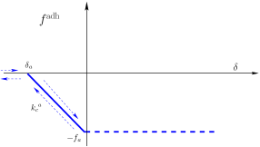
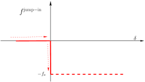
Figure 3: Schematic plots of (a) the non-contact adhesive force-overlap relation and (b) the non-contact jump-in force-overlap relation.

2.3 Non-contact normal force

It has been shown in many studies that long-range interactions are present when dry adhesive particles collide, i.e. non-contact forces are present for negative overlap $\delta$ [21, 15, 63, 93, 94]. In the previous section, we have studied the force laws for contact overlap  $\delta>0$. In this section we introduce a description for non-contact, long range, adhesive forces, focusing on the two non-contact models schematically shown in Fig. 3 – both piece-wise linear in the spirit of the mesoscopic model – namely the reversible model and the jump-in (irreversible) non-contact models (where the latter could be seen as an idealized, mesoscopic representation of a liquid bridge, just for completeness). Later, in the next section, we will combine non-contact and contact forces.

2.3.1 Reversible Adhesive force

In Fig. 3(a) we consider the reversible attractive case, where a (linear) van der Waals type long-range adhesive force is assumed. The force law can be written as

$$f^{\rm adh}=\left\{\begin{array}[]{lll}-f_{a}&&{\rm if~{}~{}}{\delta}>0\\ -k^{a}_{c}\delta-f_{a}&&{\rm if~{}~{}}0\geq{\delta}>{\delta_{a}}\\ 0&&{\rm if~{}~{}}{\delta_{a}}>{\delta}\\ \end{array}\right.$$ (14)

with the range of interaction $\delta_{a}=-{f_{a}}/{k^{a}_{c}}<0$, where $k^{a}_{c}>0$ is the adhesive “stiffness” of the material and $f_{a}>0$ is the (constant) adhesive force magnitude, active also for overlap $\delta>0$, in addition to the contact force. When $\delta=0$ the force is $-f_{a}$. The adhesive force $f^{\rm adh}$ is active when particles are closer than $\delta_{a}$, when it starts to increase/decrease linearly along $-k_{c}^{a}$, for approach/separation, respectively. In the results and theory part of the paper, for the sake of simplicity and without loss of generality, the adhesive stiffness can be either chosen as infinite, which corresponds to zero range non-contact force ($\delta_{a}=0$), or as coincident with the contact adhesive stiffness, e.g. in Sec. 2.2.2, that is $k^{a}_{c}=k_{c}$.

2.3.2 Jump-in (Irreversible) Adhesive force

In Fig. 3(b) we report the behavior of the non-contact force versus overlap when the approach between particles is described by a discontinuous (irreversible) attractive law. The jump-in force can be simply written as

$$f^{\rm jump-in}=\left\{\begin{array}[]{lll}0&&{\rm if~{}~{}}{\delta}<0\\ -f_{a}&&{\rm if~{}~{}}{\delta}\geq 0\\ \end{array}\right.~{}.$$ (15)

As suggested in previous studies [16, 21, 55], there is no attractive force before the particles come into contact; the adhesive force becomes active and suddenly drops to a negative value, $-f_{a}$, at contact, when $\delta=0$. The jump-in force resembles the limit case $k^{a}_{c}\rightarrow\infty$ of Eq. (14). Note that the behavior is defined here only for approach of the particles. We assume the model to be irreversible, as in the unloading stage, during separation, the particles will not follow this same path (details will be discussed below).

3 Coefficient of Restitution

The amount of dissipated energy relative to the incident kinetic energy is quantified by $1-e^{2}$, in terms of the coefficient of restitution $e$. Considering a pair collision, with particles approaching from infinite distance, the coefficient of restitution is defined as

$$e=\frac{{v_{f}}^{\infty}}{{v_{i}}^{\infty}}~{}$$ (16a)

where $${v_{f}}^{\infty} {v_{i}}^{\infty} v_{f} v_{i} \delta=0$$ and are final and initial velocities, respectively, at infinite separations (distance beyond which there is no long range interaction). Assuming superposition of the non-contact and contact forces, the restitution coefficient can be further decomposed including terms of final and initial velocities, and , at overlap , where the mechanical contact-force becomes active:

$$e=\frac{{v_{f}}^{\infty}}{v_{f}}\frac{v_{f}}{v_{i}}\frac{v_{i}}{{v_{i}}^{\infty}}={\epsilon_{o}}{e_{n}}{\epsilon_{i}}~{},$$ (16b)

and ${\epsilon_{i}}$ and ${\epsilon_{o}}$ are the pull-in and pull-off coefficients of restitution, that describe the non-contact parts of the interaction ($\delta<0$), for approach and separation of particles, respectively. The coefficient of restitution for particles in mechanical contact ($\delta>0$) is $e_{n}$, as analytically computed in subsection 3.3.
In the following, we will analyze each term in Eq. (16b) separately, based on energy considerations. This provides the coefficient of restitution for a wide, general class of meso interaction models with superposed non-contact and contact components, as defined in sections 2.2-2.3.

For the middle term, $e_{n}$, different contact models with their respective coefficients of restitution can be used, e.g. $e_{n}^{\rm LSD}$ from Eq. (4), $e_{n}^{\rm WB}$ from Eq. (6), or $e_{n}^{\rm HYS}$ as calculated below in subsection 3.3. Prior to this, we specify ${\epsilon_{i}}$ in subsection 3.1 and then ${\epsilon_{o}}$ in subsection 3.2, for the simplest piece-wise linear non-contact models.

3.1 Pull-in coefficient of restitution

In order to describe the pull-in coefficient of restitution $\epsilon_{i}$, we focus on the two non-contact models proposed in Sec. 2.3, as simple interpretations of the adhesive force during the approach of the particles.

When the reversible adhesive contact model is used, energy conservation leads to an increase in velocity due to the attractive branch from $\delta_{a}$ ($<0$) to contact:

$$\frac{1}{2}m_{r}{{v_{i}}^{\infty}}^{2}=\frac{1}{2}f_{a}\delta_{a}+\frac{1}{2}m_{r}{v_{i}}^{2}~{},$$ (17a)

which yields

$${\epsilon_{i}^{\rm rev-adh}}=\frac{v_{i}}{{v_{i}}^{\infty}}=\sqrt{1-\frac{f_{a}\delta_{a}}{m_{r}{{v_{i}}^{\infty}}^{2}}}=\sqrt{1+\frac{f_{a}^{2}/k_{c}^{a}}{m_{r}{{v_{i}}^{\infty}}^{2}}}~{}.$$ (17b)

The pull-in coefficient of restitution is thus larger than unity; it increases with increasing adhesive force magnitude $f_{a}$ and decreases with the adhesive strength of the material $k_{c}^{a}$ (which leads to a smaller cutoff distance).

On the other hand, if the irreversible adhesive jump-in model is implemented, a constant value $\epsilon_{i}^{\rm jump-in}=1$ is obtained for first approach of two particles, before contact, as $f^{\rm jump-in}=0$ for $\delta<0$ and the velocity remains constant $v_{i}={v_{i}}^{\infty}$.

3.2 Pull-off coefficient of restitution

The pull-off coefficient of restitution is defined for particles that lose contact and separate. Using the adhesive reversible model, as described in section 2.3.1, energy balance leads to a reduction in velocity during separation:

$$\frac{1}{2}m_{r}{{v_{f}}^{\infty}}^{2}=\frac{1}{2}f_{a}\delta_{a}+\frac{1}{2}m_{r}{v_{f}}^{2}~{},$$ (18a)

which yields

$${\epsilon_{o}}=\frac{{v_{f}}^{\infty}}{{v_{f}}}=\sqrt{1+\frac{f_{a}\delta_{a}}{m_{r}{v_{f}}^{2}}}=\sqrt{1-\frac{f_{a}^{2}/k_{c}^{a}}{m_{r}{v_{f}}^{2}}}~{},$$ (18b)

due to the negative overlap $\delta_{a}$ at which the contact ends. Similar to Eq. (17b), the pull-off coefficient of restitution depends on both the adhesive force magnitude $f_{a}$ and stiffness $k_{c}$, given the separation velocity $v_{f}$ at the end of the mechanical contact.

It is worthwhile to note that the force-overlap picture described above, with $\epsilon_{o}<1$ defined as in Eq. (18b) refers to a system with sufficiently high impact velocity, so that the particles can separate with a finite kinetic energy at the end of collision, i.e., ${v_{f}}^{2}>f_{a}^{2}/(m_{r}k_{c}^{a})=:(v_{f}^{a})^{2}$ or, equivalently, $v_{i}^{\infty}>v_{f}^{a}/(e_{n}\epsilon_{i})$, where $v_{f}^{a}$ denotes the minimal relative velocity at the end of the contact, for which particles can still separate. If the kinetic energy reaches zero before the separation, e.g. the particles start re-loading along the adhesive branch until the value $\delta=0$ is reached and the contact model kicks in.

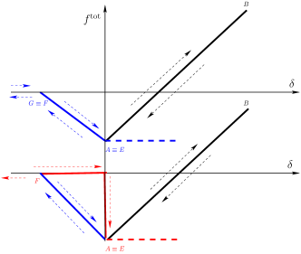
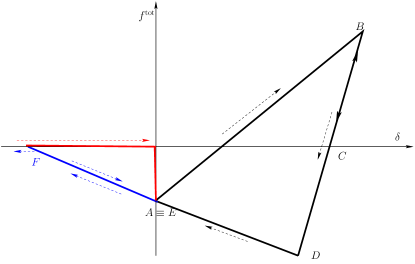
Figure 4: (a) Reversible and irreversible non-contact forces, where the top blue line (for negative overlap) represents the former and the bottom red line (for negative overlap) the latter. The black line for positive overlap represents the linear contact force as superimposed on the non-contact force. (b) Force-displacement law for elasto-plastic, adhesive contacts superimposed on the irreversible non-contact adhesive force.

3.3 Elasto-plastic coefficient of restitution

The key result of this paper is the analytical study of the coefficient of restitution as function of the impact velocity, for the model presented in Fig. 4(b), disregarding viscous forces in order to allow for a closed analytical treatment. The impact velocity $v_{i}$ is considered for two cases $v_{i}\leq v_{p}$ and $v_{i}>v_{p}$, with the plastic-limit velocity $v_{p}$ (needed to reach the elastic branch), defined as:

$$v_{p} = \sqrt{\frac{k_{1}}{m_{r}}\left[(\delta^{p}_{\rm max}-f_{a}/k_{1})^{2}-({f_{a}}/{k_{1}})^{2}\right]}$$ (19)

$$= \sqrt{\frac{1}{m_{r}}\delta^{p}_{\rm max}\left[k_{1}\delta^{p}_{\rm max}-2f_{a}\right]}~{},$$

where the term(s) with $f_{a}$ represent the energy gained or lost by this (attractive, negative) constant force, with zero reached at overlap $\delta_{a}^{(1)}=f_{a}/k_{1}$, and $\delta^{p}_{\rm max}$ defined in Eq. (10). The velocity $v_{p}$ needed to reach the limit branch thus decays with increasing non-contact attraction force $f_{a}$.

3.3.1 Plastic contact with initial relative velocity $v_{i}<v_{p}$

When $v_{i}<v_{p}$ the particles after loading to $\delta_{\rm max}$, unload with slope $k_{2}$ and the system deforms along the path $0\rightarrow\delta_{\rm max}\rightarrow\delta_{\rm 0}^{a}\rightarrow\delta_{\rm min}\rightarrow 0$, corresponding to $A\rightarrow B\rightarrow C\rightarrow D\rightarrow E$ in Fig. 4(b).

The initial kinetic energy (at $\delta=0$ overlap, with adhesive force $f_{a}$ and with initial velocity $v_{i}<v_{p}$) is completely transformed to potential energy at the maximum overlap $\delta_{\rm max}$ where energy-balance provides:

$$E_{i}:=\frac{1}{2}m_{r}v^{2}_{i}=\frac{1}{2}(k_{1}\delta_{\rm max}-f_{a})\left(\delta_{\rm max}-\frac{f_{a}}{k_{1}}\right)-\frac{1}{2}\frac{f^{2}_{a}}{k_{1}}=\frac{1}{2}\delta_{\rm max}(k_{1}\delta_{\rm max}-2f_{a})~{},$$ (20a)

so that the physical (positive) solution yields:

$$\delta_{\rm max}=\frac{f_{a}+\sqrt{f^{2}_{a}+k_{1}m_{r}v^{2}_{i}}}{k_{1}}=\delta^{(1)}_{a}+\sqrt{\left(\delta^{(1)}_{a}\right)^{2}+m_{r}v^{2}_{i}/k_{1}}~{},$$ (20b)

with zero force during loading at $$\delta^{(1)}_{a}=f_{a}/k_{1} \delta_{\rm max} B k_{2}=k_{2}(\delta_{\rm max}) C \delta^{a}_{\rm 0} f_{a}$$. The relative velocity is reversed at , and unloading proceeds from point along the slope . Part of the potential energy is dissipated, the rest is converted to kinetic energy at point , the force-free overlap , in the presence of the attractive force :

$$\frac{1}{2}m_{r}v^{2}_{0}=\frac{1}{2}(k_{1}\delta_{\rm max}-f_{a})(\delta_{\rm max}-\delta^{a}_{\rm 0})=\frac{k_{1}}{2k_{2}}\left(m_{r}v^{2}_{i}+\frac{f^{2}_{a}}{k_{1}}\right)=\frac{1}{2k_{2}}(k_{1}\delta_{\rm max}-f_{a})^{2}~{},$$ (20c)

where $$\delta^{a}_{\rm 0}=[(k_{2}-k_{1})\delta_{\rm max}+f_{a}]/{k_{2}}=:\delta_{\rm 0}+\delta^{(2)}_{a} \delta^{(2)}_{a}=f_{a}/k_{2} k_{2}(\delta_{\rm max}-\delta_{0}^{a})=k_{1}\delta_{\rm max}-f_{a}$$, with , and the second identity follows from Eq. (20a), using the force balance at the point of reversal .

Further unloading, below $\delta^{a}_{\rm 0}$, leads to attractive forces. The kinetic energy at $\delta^{a}_{\rm 0}$ is partly converted to potential energy at point $D$, with overlap $\delta_{\rm min}$, where the minimal (maximally attractive) force is reached. Energy balance provides:

$$\frac{1}{2}m_{r}v^{2}_{\rm min}=\frac{1}{2}m_{r}v^{2}_{0}-\frac{1}{2}k_{2}(\delta^{a}_{\rm 0}-\delta_{\rm min})^{2}=\frac{1}{2}m_{r}v^{2}_{0}-\frac{1}{2k_{2}}(k_{c}\delta_{\rm min}+f_{a})^{2}~{},$$ (20d)

where $\delta_{\rm min}=\frac{k_{2}\delta_{0}^{a}-f_{a}}{k_{2}+k_{c}}=\frac{(k_{2}-k_{1})\delta_{\rm max}}{k_{2}+k_{c}}$, and the second identity follows from inserting $\delta_{0}^{a}=(1+k_{c}/k_{2})\delta_{\rm min}+f_{a}/k_{2}$.

The total energy is finally converted exclusively to kinetic energy at point $E$, the end of the collision cycle (with overlap $\delta=0$):

$$\frac{1}{2}m_{r}v^{2}_{f}=\frac{1}{2}m_{r}v^{2}_{\rm min}-\frac{1}{2}k_{c}\delta^{2}_{\rm min}-f_{a}\delta_{\rm min}~{}.$$ (20e)

Using Eqs. (20c), (20d), and (20e) with the definition of $\delta_{\rm min}$, and combining terms proportional to powers of $f_{a}$ and $\delta_{\rm max}$ yields the final kinetic energy after contact:

$$E_{f}^{(1)}:=\frac{1}{2}m_{r}v^{2}_{f}=\left[\frac{k_{1}}{k_{2}}-\frac{k_{c}}{k_{1}k_{2}}\frac{(k_{2}-k_{1})^{2}}{(k_{2}+k_{c})}\right]\frac{1}{2}k_{1}\delta^{2}_{\rm max}-f_{a}\delta_{\rm max}~{},$$ (21)

with $\delta_{\rm max}$ as defined in Eq. (20b). Note that the quadratic terms proportional to $f_{a}^{2}$ have cancelled each other, and that the special cases of non-cohesive ($k_{c}=0$ and/or $f_{a}=0$) are simple to obtain from this analytical form. Finally, dividing the final by the initial kinetic energy, Eq. (20a), we have expressed the coefficient of restitution

$${e^{(1)}_{n}}=\sqrt{E_{f}^{(1)}/E_{i}}$$ (22)

as a function of maximal overlap reached, $\delta_{\rm max}$, non-contact adhesive force, $f_{a}$, elastic unloading stiffness, $k_{2}=k_{2}(\delta_{\rm max})$, and the constants plastic stiffness, $k_{1}$, and cohesive “stiffness”, $k_{c}$.

3.3.2 Plastic-elastic contact with initial relative velocity $v_{i}\geqslant v_{p}$

When the initial relative velocity $v_{i}$ is large enough such that $v_{i}\geqslant v_{p}$, the estimated maximum overlap $\delta_{\rm max}$ as defined in Eq. (20b) is greater than $\delta^{p}_{\rm max}$. Let $v_{1}$ be the velocity at overlap $\delta^{p}_{\rm max}$. The system deforms along the path $0\rightarrow\delta^{p}_{\rm max}\rightarrow\delta_{\rm max}\rightarrow\delta_{\rm 0}^{a}\rightarrow\delta_{\rm min}\rightarrow 0$.

The initial kinetic energy (at $\delta=0$ overlap, with adhesive force $f_{a}$ and with initial velocity $v_{i}\geq v_{p}$) is not completely converted to potential energy at $\delta=\delta^{p}_{\rm max}$, where energy balance provides:

$$\frac{1}{2}m_{r}v^{2}_{1}=\frac{1}{2}m_{r}v^{2}_{i}-\frac{1}{2}m_{r}v^{2}_{p}=\frac{1}{2}m_{r}v^{2}_{i}-\frac{1}{2}\delta^{p}_{\rm max}(k_{1}\delta^{p}_{\rm max}-2f_{a})~{},$$ (23a)

using the definition of $$v_{p}$$ in Eq. (19).

From this point the loading continues along the elastic limit branch with slope $k_{p}$ until all kinetic energy is transferred to potential energy at overlap $\delta_{\rm max}>\delta^{p}_{\rm max}$, where the relative velocity changes sign, i.e., the contact starts to unload with slope $k_{p}$. Since there is no energy disspated on the $k_{p}$-branch (in the absence of viscosity), the potential energy is completely converted to kinetic energy at the force-free overlap $\delta^{ap}_{0}$, on the plastic limit branch

$$\frac{1}{2}m_{r}v^{2}_{0}=\frac{1}{2k_{p}}(k_{1}\delta^{p}_{\rm max}-f_{a})^{2}+\frac{1}{2}m_{r}v^{2}_{1}~{},$$ (23b)

with the first term taken from Eq. (20c), but replacing $\delta_{\rm max}$ with $\delta^{p}_{\rm max}$ and $k_{2}$ by $k_{p}$.

Further unloading, still with slope $k_{p}$, leads to attractive forces. The kinetic energy at $\delta^{ap}_{\rm 0}$ is partly converted to potential energy at $\delta^{p}_{\rm min}$, where energy balance yields:

$$\frac{1}{2}m_{r}v^{2}_{\rm min}=\frac{1}{2}m_{r}v^{2}_{0}-\frac{1}{2}k_{p}(\delta^{ap}_{\rm 0}-\delta^{p}_{\rm min})^{2}=\frac{1}{2}m_{r}v^{2}_{0}-\frac{1}{2k_{p}}(k_{c}\delta^{p}_{\rm min}-f_{a})^{2}~{}.$$ (23c)

Some of the remaining potential energy is converted to kinetic energy so that at the end of collision cycle (with overlap $\delta=0$) one has

$$\frac{1}{2}m_{r}v^{2}_{f}=\frac{1}{2}m_{r}v^{2}_{\rm min}-\frac{1}{2}k_{c}\left(\delta^{p}_{\rm min}\right)^{2}-f_{a}\delta^{p}_{\rm min}~{},$$ (23d)

analogously to Eq. (20e)

When Eq. (23d) is combined with Eqs. (23b) and (23c), and inserting the definitions $\delta^{p}_{\rm min}=\frac{k_{p}\delta_{0}^{ap}-f_{a}}{k_{p}+k_{c}}=\frac{(k_{p}-k_{1})\delta^{p}_{\rm max}}{k_{p}+k_{c}}$, and $\delta_{0}^{ap}=(1+k_{c}/k_{p})\delta^{p}_{\rm min}+f_{a}/k_{p}$, one obtains (similar to the previous subsection):

$$E_{f}^{(2)}=\frac{1}{2}m_{r}v^{2}_{f}=\frac{1}{2}m_{r}v^{2}_{i}-\left[1-\frac{k_{1}}{k_{p}}+\frac{k_{c}}{k_{1}k_{p}}\frac{(k_{p}-k_{1})^{2}}{(k_{p}+k_{c})}\right]\frac{k_{1}}{2}\left({\delta^{p}_{\rm max}}\right)^{2}$$ (23e)

Dividing the final by the initial kinetic energy, we obtain the coefficient of restitution

$${e^{(2)}_{n}}=\sqrt{E_{f}^{(2)}/E_{i}}=:\sqrt{1-E_{\rm diss}/E_{i}}~{},$$ (24)

with constants $k_{1}$, $k_{p}$, $k_{c}$, $f_{a}$, and $\delta^{p}_{\rm max}$. Note that $e_{n}^{(2)}$, interestingly, does not depend on $f_{a}$ at all, since the constant energy $E_{\rm diss}$ is lost exclusively in the hysteretic loop (not affected by $f_{a}$). Thus, even though $E_{\rm diss}$ does not depend on the impact velocity, the coefficient of restitution does, because of its definition.

As final note, when the elastic limit regime is not used, or modified towards larger $\delta_{\rm max}^{p}$, as defined in appendix A, the limit velocity, $v_{p}$, increases, and the energy lost, $E_{\rm diss}$, increases as well (faster than linear), so that the coefficient of restitution just becomes $e^{(2)}_{n}=0$, due to complete loss of the initial kinetic energy, i.e., sticking, for all $v\leq v_{p}$.

3.4 Combined coefficient of restitution

The results from previous subsections can now be combined in Eq. (16b) to compute the coefficient of restitution as a function of impact velocity for the irreversible elasto-plastic contact model presented in Fig. 4:

$$e={\epsilon_{o}}e_{n}{\epsilon_{i}}=\left\{\begin{array}[]{lll}{\epsilon_{o}}e^{(1)}_{n}{\epsilon_{i}}&&{\rm for~{}~{}}v_{i}<v_{p}\\ {\epsilon_{o}}e^{(2)}_{n}{\epsilon_{i}}&&{\rm for~{}~{}}v_{i}\geq v_{p}\\ \end{array}\right.~{},$$ (25)

with $v_{p}$ from Eq. (19) and $\epsilon_{o}=1$ or $<0$ for reversible and irreversible non-contact forces, respectively. Note that, without loss of generality, also other shapes of non-contact, possibly long-range interactions can be used here to compute $\epsilon_{o}$ and $\epsilon_{i}$, however, going into these details goes beyond the scope of this paper, which only covers the most simple, linear non-contact force.

4 Dimensionless parameters

In order to define the dimensionless parameters of the problem, we first introduce the relevant energy scales, before we use their ratios further on:

$$\mathrm{Intial\ kinetic\ energy}:~{} {E_{i}}=\displaystyle\frac{1}{2}m_{r}v^{2}_{i}~{},$$ (26a)

$$\mathrm{Potential\ energy\ stored\ at\ \delta^{\it p}_{\rm max}}:~{} {E_{p}}=\displaystyle\frac{1}{2}k_{1}{\delta^{p}_{\rm max}}^{2}~{},$$ (26b)

$$\mathrm{Attractive\ non-contact\ potential\ energy}:~{} {E_{a}}=\displaystyle\frac{1}{2}\frac{f^{2}_{a}}{k_{1}}~{}~{}.$$ (26c)

The first two dimensionless parameters are simply given by ratios of material parameters, while last two (independent) are scaled energies:

$$\mathrm{Plasticity}:~{} \eta=\displaystyle\frac{k_{p}-k_{1}}{k_{1}}~{},$$ (27a)

$$\mathrm{Plastic\ (contact)\ adhesivity}:~{} \beta=\displaystyle\frac{k_{c}}{k_{1}}~{},$$ (27b)

$$\mathrm{Non-contact\ adhesivity}:~{} \alpha=\sqrt{\frac{E_{a}}{E_{i}}}=\sqrt{\frac{f^{2}_{a}}{k_{1}m_{r}v^{2}_{i}}}~{},$$ (27c)

$$\mathrm{Dimensionless\ (inverse)\ impact\ velocity}:~{} {\psi}=\sqrt{\frac{E_{p}}{E_{i}}}=\frac{\delta^{p}_{\rm max}}{v_{i}}\sqrt{\frac{k_{1}}{m_{r}}}~{}.$$ (27d)

from which one can derive the dependent abbreviations:

$$\mathrm{Scaled\ maximal\ deformation}:~{} \chi=\displaystyle\frac{\delta_{\rm max}}{\delta^{p}_{\rm max}}=\frac{1}{\psi}\left(\sqrt{1+\alpha^{2}}+\alpha\right)~{},$$ (28a)

$$\mathrm{Dimensionless\ impact\ velocity}:~{} {\zeta}=\frac{v_{i}}{v_{p}}=\frac{1}{\sqrt{\psi^{2}-2\alpha\psi}}~{}.$$ (28b)

Using Eqs. (27a), (27b) and (28a), $k_{2}$ can be rewritten in non-dimensional form

$$\frac{k_{2}(\chi)}{k_{1}}=\left\{\begin{array}[]{lll}1+\eta\chi,&{\rm~{}if~{}}\chi<1\\ 1+\eta,&{\rm~{}if~{}}\chi\geq 1\end{array}\right.~{},$$ (29)

so that Eq. (22) becomes:

$$e^{(1)}_{n}=\sqrt{\left(\frac{1}{1+\eta\chi}-\frac{\beta\eta^{2}\chi^{2}}{(1+\eta\chi)(1+\beta+\eta\chi)}\right)\psi^{2}\chi^{2}-2\alpha\psi\chi}~{},$$ (30)

and, similarly, Eq. (24) in non-dimensional form reads:

$$e^{(2)}_{n}=\sqrt{1-\left(1-\frac{1}{1+\eta}+\frac{\beta\eta^{2}}{(1+\eta)(1+\beta+\eta)}\right)\psi^{2}}~{},$$ (31)

where the abbreviation $\psi\chi=\left(\sqrt{1+\alpha^{2}}+\alpha\right)$ was used.

To validate our analytical results, we confront our theoretical predictions with the results of two-particle DEM simulations in Fig. 5, which shows $e$ plotted against the dimensionless impact velocity $\zeta$, for elasto-plastic adhesive spheres with different non-contact adhesion strength $f_{a}$ (and thus $\alpha$). The lines are the analytical solutions for the coefficient of restitution, see Eqs. (30) and (31), and the symbols are simulations, with perfect agreement, validating our theoretical predictions.

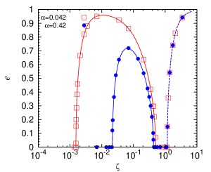
Figure 5: Restitution coefficient $e$ plotted as a function of the dimensionless impact velocity $\zeta$, see Eq. (28b), for elasto-plastic adhesive spheres with the irreversible non-contact branch. Solid and dashed lines correspond to the analytical expressions in Eqs. (30) and (31), respectively, and the squares and circles are results of DEM simulations for values of $f_{a}$ as given in the legend in terms of $\alpha=0.042$ and $0.42$ (for impact velocity $v_{i}=0.01$ ms^-1). Simulation parameters used here are $k_{1}=10^{2}$ Nm^-1, $k_{p}=5\times 10^{2}$ Nm^-1, ($\eta=4$), $k_{c}=10^{2}$ $\mathrm{Nm^{-1}}$, ($\beta=1$), with $\phi_{f}=0.1$, for particles with radius $1.1\times 10^{-3}$ m, density $2000$ kg/m³, and thus mass $m_{r}=5.6\times 10^{-6}$ kg.

For low velocity, the coefficient of restitution $e$ is zero, i.e., the particles stick to each other. This behavior is in qualitative agreement with previous experimental and numerical results [54, 21, 56]. With increasing impact velocity, $e$ begins to increase and then decreases again, displaying a second sticking regime (for the parameters used here). For even higher impact velocity, $v>v_{p}$ (and thus $\zeta>1$), another increase is observed, which will be explained in more detail in the next section.

Besides the onset of the plastic-limit regime at $\zeta=1$, we observe three further velocities $\zeta_{c}^{(a)}$, $\zeta_{c}^{(b)}$ and $\zeta_{c}^{(c)}$, for the end of the first sticking regime, i.e. $0\leq\zeta\leq\zeta_{c}^{(a)}$, and the second sticking regime, i.e. $\zeta_{c}^{(b)}\leq\zeta\leq\zeta_{c}^{(c)}$. While $\zeta_{c}^{(c)}$ is constant, the critical velocity, $\zeta_{c}^{(a)}$, required to separate the particles increases, whereas $\zeta_{c}^{(b)}$, required to enter the high-velocity sticking regime, decreases with the non-contact adhesion $f_{a}$.

The further study of these critical velocities and the comparison to existing literature (theories and experiments) goes beyond the scope of the present study, since there are just too many possibilities for materials and particle sizes. We only refer to one example, where the end of the low-velocity sticking regime was predicted as a non-linear function of the surface energy/adhesion [26] and hope that our proposal of using dimensonless numbers will in future facilitate calibration of contact models with both theories and experiments.

5 Results using the mesoscopic contact model only ($f_{a}=0$)

Having understood the results for the contact model with finite non-contact force $f_{a}$, we will restrict our analytical study to the special case of negligible non-contact adhesive forces $f_{a}=0$, in the following, which corresponds to the range of moderate to large impact velocity or weak $f_{a}$, i.e. $\alpha\ll 1$.

For this special case, the dimensionless parameters reduce to $\alpha=0$, and $\chi=\frac{1}{\psi}=\zeta=\frac{v_{i}}{v_{p}}$. The expressions for the coefficients of restitution presented in Eqs. (30) and (31) reduce to

$$e^{(1)}_{n}(\eta,\beta,\chi\leq 1)=\sqrt{\frac{1}{1+\eta\chi}-\frac{\beta\eta^{2}\chi^{2}}{(1+\eta\chi)(1+\beta+\eta\chi)}}$$ (32)

and

$$e^{(2)}_{n}(\eta,\beta,\chi>1)=\sqrt{1-\left[1-e^{(1)}_{n}(\eta,\beta,\chi=1)^{2}\right]\frac{1}{\chi^{2}}}~{}.$$ (33)

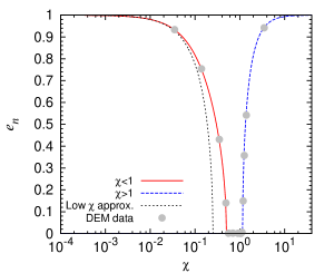
Figure 6: Restitution coefficient plotted as a function of the scaled initial velocity $\chi$ for a collision without viscous and non-contact forces ($\alpha=0$). The solid red line corresponds to the analytical expression in Eq. (32), the dashed blue line to Eq. (33), the thin black line represents the low velocity approximation, and the circles are DEM simulation data. The material parameters are as in Fig. 5, i.e. $\eta=4$ and $\beta=1$.

5.1 Qualitative Description

In Fig. 6, the analytical prediction for the coefficient of restitution, from Eqs. (32) and (33), is compared to the numerical integration of the contact model, for different scaled initial velocities $\chi$. We confirm the validity of the theoretical prediction for the coefficient of restitution in the whole range.

For very small $\chi<10^{-2}$, the approximation $e^{(1)}_{n}\approx{1-\frac{\eta\chi}{2}}$ predicts the data very well. With increasing initial relative velocity, dissipation increases non-linearly with the initial kinetic energy, leading to a convex decrease of $e^{(1)}_{n}$ (due to the log-scale plot). The coefficient of restitution $e^{(1)}_{n}$ becomes zero when a critical scaled initial velocity $\chi^{(b)}_{c}$ (see Eq. (34) below) is reached. At this point, the amount of dissipated energy becomes equal to the initial kinetic energy, leading to sticking of particles. The coefficient of restitution remains zero until a second critical scaled initial velocity $\chi^{(c)}_{c}$ is reached, i.e. sticking is observed for $\chi^{(b)}_{c}\leq\chi\leq\chi^{(c)}_{c}$. Finally, for $\chi>\chi^{(c)}_{c}$, the dissipated energy remains constant (the elastic limit branch is reached), while the initial kinetic energy increases. As a result, the kinetic energy after collision increases and so does the coefficient of restitution $e_{n}$. Existence of sticking at such high velocities was recently reported by Kothe et al. [99], who studied the outcome of collisions between sub-mm-sized dust agglomerates in micro-gravity [26] . Note that an increase of $e_{n}$ for high velocity is a familiar observation in studies focused on the cold-spray technique [2, 3, 4]. Above a certain (critical) velocity the spray particles adhere to the substrate, and they do so for a range of impact velocities; increasing the impact velocity further leads to unsuccessful deposition, i.e. the particles will bounce from the substrate. The sticking and non-sticking phenomenology of such materials has been extensively studied experimentally and numerically in Refs. [2, 3, 4, 5, 6].

In Fig. 7, we compare the variation of the force with overlap in the various regimes of $\chi$ as discussed above, but here for $\phi_{f}=0.05$. For very small $\chi$, the unloading slope $k_{2}\approx k_{1}$, (see Fig. 7(a) for a moderate $\chi=0.34$), and the amount of dissipated energy is small, increasing with $\chi$. The kinetic energy after collision is almost equal to the initial kinetic energy, i.e. $e_{n}\sim 1$, see Fig. 6. In Figs. 7(b) and 7(c), the force-overlap variation is shown for sticking particles, for the cases $\chi^{(b)}_{c}<\chi<1$ and $1<\chi<\chi^{(c)}_{c}$, respectively (more details will be given in the following subsection). Finally, in Fig. 7(d), the case $\chi>\chi^{(c)}_{c}$ is displayed, for which the initial kinetic energy is larger than the dissipation, resulting in separation of the particles. The corresponding energy variation is described in detail in appendix B.

   

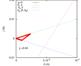
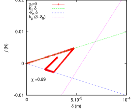
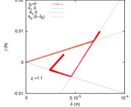
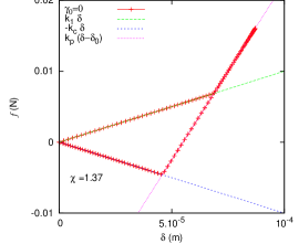
Figure 7: Contact force during one collision, plotted against the overlap for different scaled initial velocities $\chi=0.34$, 0.69, 1.1, and 1.37, respectively. The three straight lines represent the plastic branch, with slope $k_{1}$, the adhesive branch, with slope $-k_{c}$, and the limit branch with slope $k_{p}$, for $k_{1}=10^{2}$ Nm^-1, $k_{p}=5\times 10^{2}$ Nm^-1, $k_{c}=10^{2}$ $\mathrm{\,Nm^{-1}}$, i.e. $\eta=4$ and $\beta=1$, and $\phi_{f}=0.05$.

5.2 Sticking regime limits and overlaps

In this section we focus on the range of $\chi^{(b)}_{c}<\chi\leq\chi^{(c)}_{c}$, where the particles stick to each other (implying that $\beta$ is large enough $\beta\geq\beta^{*}$ with minimal $\beta^{*}$ for sticking) and calculation of the critical values $\chi^{(b)}_{c}$ and $\chi^{(c)}_{c}$. When $\chi=\chi^{(b)}_{c}$ all of the initial kinetic energy of the particles is just dissipated during the collision. Hence the particles stick and $e^{(1)}_{n}(\eta,\beta,\chi^{(b)}_{c})=0$, which leads to $1+\beta+\eta\chi-\beta\eta^{2}\chi^{2}=0$. Only the positive solution is physically possible, as particles with negative initial relative velocity cannot collide, so that

$$\chi^{(b)}_{c}=\frac{1}{2\beta\eta}\left[1+\sqrt{1+4\beta(1+\beta)}\right]~{}$$ (34)

is the lower limit of the sticking regime. For larger $\chi>\chi^{(b)}_{c}$, the dissipation is strong enough to consume all the initial kinetic energy, hence the particles loose their kinetic energy at a positive, finite overlap $\delta_{\rm c}$, see Fig. 7(b). The contact deforms along the path $0\rightarrow\delta_{\rm max}\rightarrow\delta_{\rm 0}\rightarrow\delta_{\rm min}\rightarrow\delta_{\rm c}$. Thereafter, in the absence of other sources of dissipation, particles keep oscillating along the same slope $k_{2}$. In order to compute $\delta_{\rm c}$, we use the energy balance relations in Eqs. (20), and conservation of energy along $\delta_{\rm min}\rightarrow\delta_{\rm c}$, similar to Eq. (20e),

$$\frac{1}{2}m_{r}v^{2}_{\rm min}-\frac{1}{2}k_{c}\left\{\delta_{\rm min}^{2}-\delta^{2}_{\rm c}\right\}=0~{},$$ (35a)

with vanishing velocity $$v_{c}=0 \delta_{c} k_{c} \delta_{\rm max}$$ at overlap . Using the definitions around Eqs. (20) and re-writing in terms of and leads to

$$k_{c}\delta^{2}_{\rm c}+\left\{\frac{k^{2}_{1}}{k_{2}}-\frac{k_{c}(k_{2}-k_{1})^{2}}{k_{2}(k_{2}+k_{c})}\right\}\delta^{2}_{\rm max}=0$$ (35b)

and thus to the sticking overlap in regime (1), for $$\chi^{(b)}_{c}v_{p}<v_{i}<v_{p}$$:

$$\frac{\delta^{(1)}_{\rm c}}{\delta^{p}_{\rm max}}=\frac{\delta_{\rm max}}{\delta^{p}_{\rm max}}\sqrt{\frac{(k_{2}-k_{1})^{2}}{k_{2}(k_{2}+k_{c})}-\frac{k^{2}_{1}}{k_{2}k_{c}}}~{}.$$ (35c)

In terms of dimensionless parameters, as defined earlier, this can be written as:

$$\frac{\delta^{(1)}_{\rm c}}{\delta^{p}_{\rm max}}=\chi\sqrt{\frac{\eta^{2}\chi^{2}}{(1+\eta\chi)(1+\beta+\eta\chi)}-\frac{1}{\beta(1+\eta\chi)}}=\frac{\chi}{\sqrt{\beta}}\hat{e}_{n}^{(1)}~{},$$ (36)

where $\hat{e}_{n}^{(1)}$ denotes the result from Eq. (32) with positive argument under the root.

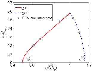
Figure 8: Kinetic energy-free contact overlap $\delta_{\rm{}_{c}}$ plotted as a function of the scaled initial velocity $\chi={v_{i}}/{v_{p}}$; the increasing branch corresponds to $\chi<1$, while the decreasing branch corresponds to $\chi>1$. The dots are simulations for $\eta=4$ and $\beta=1$, as in Fig. 7, which yields $\delta^{\rm max}_{\rm{}_{c}}/{\delta^{p}_{\rm max}}=(1/3)^{1/2}$ in Eq. (39).

For larger initial relative velocities, $\chi\geq 1$, the coefficient of restitution is given by Eq. (33), so that the upper limit of the sticking regime $\chi^{(c)}_{c}>1$ can be computed by setting $e^{(2)}_{n}(\eta,\beta,\chi^{(c)}_{c})=0$. Again, only the positive solution is physically meaningful, so that

$$\chi^{(c)}_{c}=\sqrt{1-\frac{1}{1+\eta}+\frac{\beta\eta^{2}}{(1+\eta)(1+\beta+\eta)}}$$ (37)

is the maximum value of $\chi$ for which particles stick to each other. For $\chi\leqslant\chi^{(c)}_{c}$ particles deform along the path $0\rightarrow\delta^{p}_{\rm max}\rightarrow\delta_{\rm max}\rightarrow\delta_{\rm 0}\rightarrow\delta_{\rm min}\rightarrow\delta_{\rm c}$ and then keep oscillating on the branch with stiffness $k_{2}$, with $\delta_{\rm c}$ being one of the extrema of the oscillation, see Fig. 7(c). Similar to the considerations above, we compute the sticking overlap in regime (2), for $v_{p}<v_{i}<\chi^{(c)}_{c}v_{p}$: in dimensionless parameters:

$$\frac{\delta^{(2)}_{\rm c}}{\delta^{p}_{\rm max}}=\sqrt{\frac{\eta^{2}}{(1+\eta)(1+\beta+\eta)}+\frac{\eta}{\beta(1+\eta)}-\frac{\chi^{2}}{\beta}}=\frac{\chi}{\sqrt{\beta}}\hat{e}_{n}^{(2)}~{},$$ (38)

where $\hat{e}_{n}^{(2)}$ denotes the result from Eq. (33) with positive argument under the root.

In Fig. 8, the scaled sticking overlap ${\delta_{\rm{}_{c}}}/{\delta^{p}_{\rm max}}$ is plotted for different $\chi$, showing perfect agreement of the analytical expressions in Eqs. (36) and (38), with the numerical solution for a pair-collision. In the sticking regime, the stopping overlap increases with $\chi$, and reaches a maximum at $\chi=1$,

$$\frac{\delta_{\rm{}_{c}}({\chi=1})}{\delta^{p}_{\rm max}}=\sqrt{\frac{\beta\eta^{2}-(1+\eta+\beta)}{\beta(1+\eta)(1+\eta+\beta)}}$$ (39)

which depends on the the adhesivity $\beta$ and the plasticity $\eta$ only. For $\chi>1$, dissipation gets weaker, relatively to the increasing initial kinetic energy, and $\delta^{(2)}_{\rm{}_{c}}/{\delta^{p}_{\rm max}}$ decreases until it reaches $0$ for $\chi=\chi^{(c)}_{c}$.

5.3 Contacts for different adhesivity $\beta$

In the previous subsections, we studied the dependence of the coefficient of restitution $e_{n}$ on the scaled initial velocity $\chi$ for fixed adhesivity $\beta$, whereas here the dependence of $e_{n}$ on $\beta$ is analyzed.

A special adhesivity $\beta^{*}$ can be calculated such that $e_{n}=0$ for $\chi=1$, which is the case of maximum dissipation, and leads to sticking only at exactly $\chi=1$, i.e. there is no sticking for $\beta<\beta^{*}$. Using Eq. (32), we get

$$1+\beta^{*}+\eta-\beta^{*}\eta^{2}=0~{},$$ (40a)

so that

$$\beta^{*}=\frac{1}{\eta-1}~{}.$$ (40b)

In Fig. 9, we plot the coefficient of restitution $e$ as a function of the scaled initial velocity $\chi$ for different values of adhesivity $\beta$. For $\beta<\beta^{*}$, in Fig. 9, the coefficient of restitution $e_{n}$ decreases with increasing $\chi<1$, reaches its positive minimum at $\chi=1$, and increases for $\chi>1$. In this range, the particles (after collision) always have a non-zero relative separation velocity $v_{f}$. When $\beta=\beta^{*}$, $e_{n}$ follows a similar trend, becomes zero at $\chi=1$, and increases with increasing scaled initial velocity for $\chi>1$. This is the minimum value of adhesivity for which $e_{n}$ can become zero and particles start to stick to each other. For $\beta=\beta^{*}$, the sticking regime upper and lower limits coincide, $\chi^{(b)}_{c}=\chi^{(c)}_{c}=1$. If $\beta>\beta^{*}$, $e_{n}$ decreases and becomes zero at $\chi=\chi^{(b)}_{c}<1$, it remains zero until $\chi=\chi^{(c)}_{c}>1$, and increases with increasing relative initial velocity thereafter. Hence, the range of velocities for which sticking happens is determined by the material properties of the particles. Indeed Zhou et al. [6] presented similar conclusions about the deposition efficiency in cold spray. Simulations with viscous forces change the value of $\beta^{*}$ and are not shown here, see Appendix B.

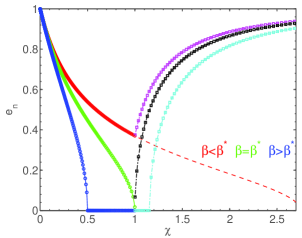
Figure 9: Coefficient of restitution $e_{n}$ plotted against the scaled initial velocity $\chi$. Circles with different colors correspond to different adhesivity $\beta$ (red for $\beta<\beta^{*}$, green for $\beta=\beta^{*}$ and blue for $\beta>\beta^{*}$) for $\chi\leq 1$ , while magenta, black and cyan squares correspond to the respective values of $\beta$ for $\chi>1$. Other parameters used are $k_{1}=10^{2}$, $k_{p}=5\times 10^{2}$, and different $k_{c}$ (all in units of $\mathrm{Nm^{-1}}$), i.e. $\eta=4$ and $\beta/\beta^{*}=1/3$, $1$, and $3$, with $\beta^{*}=1/3$. The dashed red line represents the solution with the tuned fully plastic model with a new ${\phi_{f}}^{{}^{\prime}}=0.5$ and newly calculated ${k_{p}}^{{}^{\prime}}$, see Appendix A .

6 Conclusions and outlook

Various classes of contact models for non-linear elastic, adhesive and visco-elasto-plastic particles are reviewed. Instead of focusing on the well understood models for perfect spheres of homogeneous (visco) elastic or elasto-plastic materials, a special mesoscopic adhesive (visco) elasto-plastic contact model is considered, aimed at describing the macroscale behavior of assemblies of realistic fine particles (different from perfectly homogeneous spheres). An analytical solution for the coefficient of restitution of pair-contacts is given as reference, for validation, and to understand the role of the contact model parameters.

Mesoscopic Contact Model

The contact model by Luding [15], including short-ranged (non-contact) interactions, is critically discussed and compared to alternative approaches in subsection 1.2. The model introduced in section 2 is simple (piece-wise linear), yet it catches the important features of particle interactions that affect the bulk behavior of a granular assembly, i.e. non-linear elasticity, plasticity and contact adhesion. It is mesoscopic in spirit, i.e. it does not resolve all the details of every single contact, but is designed to represent an ensemble of particles with many contacts in a bulk system. One goal of this study is to present this rich, flexible and multi-purpose granular matter meso-model, which can be calibrated to realistically model ensembles of large numbers of particles [100]. The analytical solution for the contact dissipation is given for contact and non-contact forces both active, but viscosity inactive, in section 3. A sensible set of dimensionless parameters is defined in section 4, before the influence of the model parameters on the overall impact behavior is discussed in detail, focusing on the irreversible, adhesive, elasto-plastic part of the model, in section 5.

Analysis of the coefficient of restitution

When the dependence of the coefficient of restitution, $e$, on the relative velocity between particles is analyzed, two sticking regimes, $e=0$, show up, as related to different sources of dissipation:

(i) As previously reported in the literature (see e.g. Refs. [52, 55, 21, 56, 62]) the particles stick to each other at very low impact velocity. This can happen due to irreversible short-range non-contact interaction, as e.g. liquid bridges, or due to van der Waals type force for dry adhesive particles. The threshold velocity, below which the particles stick depends on the magnitude of the non-contact adhesive force $f_{a}$, while for elasto-plastic adhesive particles on both non-contact adhesive force and plasticity, which together control this low-velocity sticking.

(ii) With increasing velocity, $e$ increases and then decreases until the second sticking regime is reached, which is strongly influenced by the plastic/adhesive (and viscous) dissipation mechanisms in the hysteretic contact meso-model. At small impact velocity, all details of the model are of importance, while at higher velocities, for a sufficiently low value of the jump-in force $f_{a}$, the contribution of the non-contact forces can be neglected. The theoretical results are derived in a closed analytical form, and phrased completely in terms of dimensionless parameters (plasticity, adhesivity and initial velocity). The ranges of impact velocities for the second sticking regime are predicted and discussed in detail.

(iii) For still increasing relative velocity, beyond the second sticking region, $e$ starts increasing again. This regime involves a change of the physical behavior of the system as expected, e.g. for non-homogeneous materials with micro-structure and non-flat contacts, or materials with an elastic core, e.g. asphalt (stone with bitumen layer). Even though this elastic limit behavior is a feature of the model, completely plastic behavior can be reproduced by the model too, just by tuning two input parameters $k_{p}$ and $\phi_{f}$, as shown in appendix A. This way, the low velocity collision dynamics is kept unaffected, but the elastic limit regime is reached only at higher impact velocities, or can be completely removed. This modification provides the high velocity sticking regime for all high velocities, as expected for ideally plastic materials. On the other hand, the existence of a high velocity rebound, as predicted the model with elastic limit regime, has been observed experimentally and numerically in cold spray [2, 3, 4, 5, 6] and can be expected for elastic core with a thin plastic shell.

Additional dissipative mechanisms

For sticking situations, on the un-/re-loading branch, the particles oscillate around their equilibrium position until their kinetic energy is dissipated, since realistic contacts are dissipative in nature. Since viscosity hinders analytical solutions, it was not considered before, but a few simulation results with viscosity are presented in Appendix B. With viscosity, both un- and re-loading are not elastic anymore, resembling a damped oscillation and eventually leading to a static contact at finite overlap.

Application to multi-particle situations

The application of the present meso-model to many-particle systems (bulk behavior) is the final long-term goal, see e.g. Ref. [28, 29, 35], as examples, where the non-contact forces were disregarded. An interesting question that remains unanswered concerns a suitable analogy to the coefficient of restitution (as defined for pair collisions) relevant in the case of bulk systems, where particles can be permanently in contact with each other over long periods of time, and where impacts are not the dominant mode of interaction, but rather long lasting contacts with slow loading-unloading cycles prevail.

One specific example for the latter situation of slow loading-unloading of bulk material is given in Appendix F, showing qualitatively similar behavior as encompassed in the contact meso-model, but on a much larger length-scale than the contact model itself, highlighting the dominant role of the particle structure and the (non-flat) contact area with related plastic (irreversible) re-arrangements [26].

Outlook

The interest of widely different communities (viz. particle technology, granular physics, interstellar dust, asphalt, or cold-spray) in the dependence of the coefficient of restitution (or deposition/impact behavior) on the impact velocity is considerable. We hope our study helps to connect these widely different communities by providing an overview and, in particular, a flexible, multi-purpose contact model, valid and useful for many practically relevant situations.

The contact meso-model has to be calibrated for different materials, while our reference analytical results allow to verify the model implementation. With this, the model can be used to predict bulk material behavior and to be validated by comparison with experiments.

7 Acknowledgment

Insightful discussions with L. Brendel, M. Ghadiri, N. Kumar, S. Li, M. Pasha, H. Tanaka, S. Thakur C. Thornton, J. Tomas, O. Walton, and T. Weinhart are highly appreciated.

Financial support (project number: 07CJR06) from the research program “Jamming and Rheology” of the Stichting voor Fundamenteel Onderzoek der Materie (FOM), and of the STW-VICI project (number 10828) “Bridging the gap between Discrete and Continuous systems”, both financially supported by the “Nederlandse Organisatie voor Wetenschappelijk Onderzoek” (NWO), is acknowledged.

Appendix A Tuning of parameters to increase the plastic range

We assume that the reference dimensionless plasticity depth be $\phi_{f}$, which is, e.g. calculated based on the maximal volume fraction related arguments of a multi-particle assembly, and $k_{p}$ be the reference limit stiffness. We propose a new ${\phi_{f}}^{{}^{\prime}}>{\phi_{f}}$, which represents the new (larger) dimensionless plasticity depth (arbitrary choice or calculated based on another volume fraction consideration) and a new value of ${k_{p}}^{{}^{\prime}}$; the choice is such that the tuned model resembles exactly, consistently, the reference for $\delta_{0}<a_{12}\phi_{f}$, with reduced radius $a_{12}$, and becomes plastic for $a_{12}\phi_{f}<\delta_{0}<a_{12}{\phi_{f}}^{{}^{\prime}}$. At $\delta_{0}=a_{12}\phi_{f}$, Eq. (10) reads

$$k_{p}=k_{1}+({k_{p}}^{{}^{\prime}}-k_{1}){\delta^{p}_{\rm max}}/{{\delta^{p}_{\rm max}}}^{{}^{\prime}},$$ (A.1)

since all parameters except $\phi_{f}$ and $k_{p}$ remain unchanged. Using Eqs. (A.1) and (11) we arrive at

$$\frac{(k_{p}-k_{1})^{2}}{k_{p}\phi_{f}}=\frac{({k_{p}}^{\prime}-k_{1})^{2}}{{k_{p}}^{\prime}{\phi_{f}}^{\prime}},$$ (A.2)

which gives the new limit stiffness

$${k_{p}}^{{}^{\prime}}=k_{1}+{AB}/{2}+\sqrt{(AB/2)^{2}+k_{1}AB},$$ (A.3)

where $A={(k_{p}-k_{1})^{2}}/{k_{p}}$ and $B={{\phi_{f}}^{{}^{\prime}}}/{\phi_{f}}$.

Using Eq. (A.3), we can calculate values of the new limit plastic stiffness ${k_{p}}^{{}^{\prime}}$ for any given ${\phi_{f}}^{{}^{\prime}}$, such that the collision dynamics for lower plastic deformation $\delta_{0}<{\delta^{p}}_{0}$ is intact, while the range of plastic deformation is enhanced, depending on the chosen ${\phi_{f}}^{{}^{\prime}}>{\phi_{f}}$.

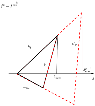
Figure 10: Force-displacement law for elasto-plastic, adhesive contacts superimposed on the irreversible contact force law. The black solid line represents the force law for reference input parameters $\phi_{f}$ and $k_{p}$, while the dashed red line represents the same for a new chosen ${\phi_{f}}^{{}^{\prime}}$ and newly calculated ${k_{p}}^{{}^{\prime}}$ resembling a wider plastic regime of the particle deformation.

Appendix B Effect of Viscosity

Since real physical systems also can have additional dissipation modes that are, e.g. viscous in nature, we study the behavior of collisions with viscous damping present ($\gamma_{0}>0$) and compare it with the non-viscous case ($\gamma_{0}=0$). Note that any non-linear viscous damping force can be added to the contact laws introduced previously, however, for the sake of simplicity we restrict ourselves to the simplest linear viscous law as given as second term in Eq. (2), since it can be important to choose the correct viscous damping term for each force law to get the physically correct behavior [46, 101, 74, 50]. In Fig. 11, we plot the contact force against the overlap, and the overlap against time, during collisions for a constant value of $\chi=1$ and different $\beta$, for $\gamma_{0}=5\times 10^{-3}$ kg s^-1.

When $\beta<\beta^{*}$, see Fig. 11(a) and Fig. 11(b), the contact ends when the adhesive force $-k_{c}\delta$ goes back to zero, for both cases, with and without viscosity. This is since the viscosity is relatively small and does not contribute enough to the total dissipation to make the particles stick for the parameters used here.

For the critical adhesivity $\beta=\beta^{*}$, reported in Fig. 11(c), without viscosity, the overlap between the particles goes down to exactly zero at the end of the collision, with all kinetic energy dissipated. For $\gamma_{0}>0$, dissipation brings this marginal case into the sticking regime and the particles stay in contact at $\delta>0$. This can be seen clearly in Fig. 11(d), where the particles undergo a damped oscillatory motion due to the small residual velocity created on the re-loading branch.

For larger values $\beta>\beta^{*}$, the overlap at which kinetic energy is lost completely (on the $k_{c}$ branch) is finite, for both $\gamma_{0}=0$ and $\gamma_{0}>0$, see Fig. 11(e). In both cases, the particles stick and remain in contact. Without viscosity, the particles keep oscillating along the slope $k_{2}$, while with viscosity the oscillation is damped and kinetic energy vanishes. During loading and unloading the apparent slope changes with time due to the additional viscous force that leads to the dissipation of energy, as evident from the ellipsoidal converging spiral. Waiting long enough, for some oscillation cycles, the particles stick to each other with a finite overlap and zero relative kinetic energy. The difference is also visible in Fig. 11(f), where for $\gamma_{0}=0$ the particles keep oscillating with constant amplitude, whereas, for $\gamma_{0}>0$, the particles undergo a damped oscillatory motion, until the velocity becomes $0$ at $\delta>0$. The time evolution of the overlap in Fig. 11(f) resembles that of the displacement evolution in Ref. [102], where the authors studied sticking of particles in Saturn’s rings.

     

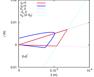
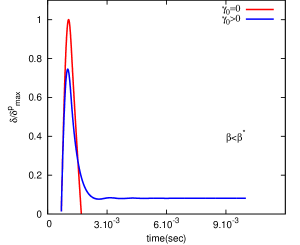
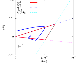
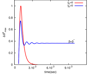
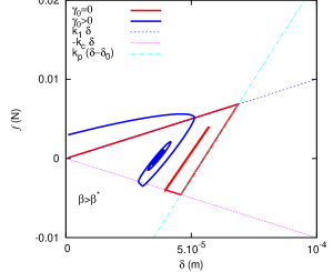
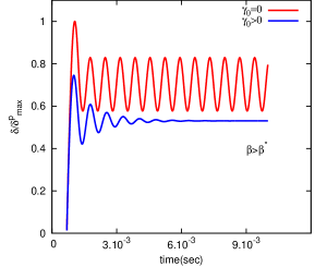
Figure 11: (a), (c), (e) Contact forces plotted against overlap and (b), (d), (f) time evolution of ${\delta}/{\delta^{p}_{\rm max}}$ for pair collisions with parameters $k_{1}=10^{2}$, $k_{p}=5\times 10^{2}$ and different $k_{c}=10$, $33.33$, and $100$, (units $\mathrm{Nm^{-1}}$), i.e. with $\eta=4$, $\beta<\beta^{*}$, $\beta=\beta^{*}$ and $\beta>\beta^{*}$, for the same situations as shown in Fig. 9. The red and blue lines represent the data in the presence and absence of viscosity respectively, where $\gamma_{0}=5\times 10^{-3}$, (unit $\mathrm{Nm^{-1}sec}$).

Appendix C Asymptotic Solutions

In this subsection, we focus on the case $\chi\leq 1$, and study the asymptotic behavior of the coefficient of restitution as function of the impact velocity.

For the sake of simplicity, let us start with an elasto-plastic system without adhesion, i.e. $k_{c}=0$, in Eq. (32) such that

$$e^{(1)}_{n}(\eta,\beta=0,\chi<1)=\sqrt{\frac{1}{1+\eta\chi}},$$ (C.1a)

inserting the definitions of $$\eta \beta v_{p}$$, and ,

$$e^{(1)}_{n}(\beta=0,v<v_{p})=\sqrt{\dfrac{1}{1+\dfrac{k_{p}-k_{1}}{k_{1}}\dfrac{v_{i}}{\sqrt{{\dfrac{2k_{1}}{m}}}{\delta^{p}_{\rm max}}}}},$$ (C.1b)

using Eq. (12), where we defined $$S=\frac{k_{p}-k_{1}}{k_{1}{\delta^{p}_{\rm max}}} \omega_{o}=\sqrt{\frac{2k_{1}}{m}}$$ and assuming , we get

$$e^{(1)}_{n}(\beta=0,v<v_{p})=\sqrt{\frac{1}{1+\frac{Sv_{i}}{\omega_{0}}}}.$$ (C.1c)

Eq. (C.1c) is exactly the same as Eq. (5) in [71]. For non-cohesive particles, and in the range $v<v_{p}$ we get exactly the same solution as Walton and Braun [71].

Further to study the asymptotic solution

$$e^{(1)}_{n}(\eta,\beta=0,\chi<1)=\sqrt{\frac{1}{1+\eta\chi}}\approx(\eta\chi)^{-1/2}$$ (C.2)

with the approximation valid for $\eta\chi\gg 1$.

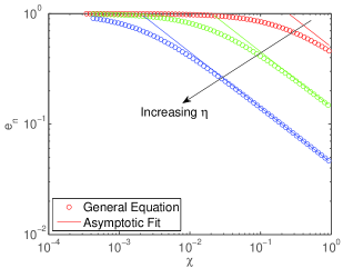
Figure 12: The coefficient of restitution is plotted against the scaled initial velocity $\chi$ in log-log-scale for $\beta=0$ and three values of $\eta=5$, $50$, and $500$, with the other parameters as in Fig. 6. Red, green and blue circles denote, respectively, the solution of Eq. (C.2), while the solid lines represent the approximation for high scaled impact velocity and large plasticity $\eta\gg 1$.

Since the scaled velocity is moderate, $\chi<1$, the condition requires a large plasticity, i.e., a strong difference between the limit stiffness and the plastic loading stiffness, $\eta\gg 1$ (or $k_{p}\gg k_{1}$). In Fig. 12, we plot the coefficient of restitution against the scaled initial velocity $\chi$ for three different values of $\eta=k_{p}/k_{1}$, together with the power law prediction of Eq. (C.2). We observe, that for the smallest $\eta$ (red circle and line), the approximation is far from the data, while for higher $\eta$, the approximation works well even for rather small velocities $\chi\approx 0.1$.

Next, when studying the elasto-plastic adhesive contact model, $\beta>0$ and $\beta\ll 1$, again, we restrict ourselves to values of $\eta$ such that asymptotic condition $\eta\chi\gg 1$ is satisfied. Hence, Eq. (32) can be approximated as

$$e^{(1)}_{n}(\eta,\beta,\chi<1)\approx\sqrt{\frac{1}{\eta\chi}-\beta}~{},$$ (C.3)

as long as $\eta\chi\gg\beta\geq 0$ and $\frac{1}{\eta}>\beta$ holds.

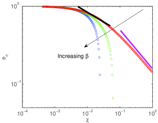
Figure 13: Log-log plot of the coefficient of restitution against the scaled initial velocity $\chi$ for four different values of $\beta=0.01$, $0.1$, and $1.0$, with $\eta=50$. Red, green and blue circles denote the respective solutions of the general equation, Eq. (32), solid black line represents power law $e_{n}\sim v^{-1/4}$, while magenta line denotes $e_{n}\sim v^{-1/2}$.

In Fig. 13, we plot the coefficient of restitution against the scaled initial velocity $\chi$ for different values of $\beta$ and superimpose the approximation, Eq. (C.3). For small $\beta$ and large $\chi$, one observes good agreement between the full solution and the approximation. Differently, for the highest values of $\beta$ the approximation is not valid. Due to the adhesive force, for large $\chi$, with increasing $\beta$, the deviation from the $\chi^{-1/2}$ power law becomes increasingly stronger, leading to the sticking regime, as discussed in the previous subsections. On the other hand, for smaller velocities, one observes a considerably smaller power-law, resembling the well-known $\chi^{-1/4}$ power law for plastic contacts, as indicated by the dashed line in Fig. 13.

Appendix D Dependence on interpolation

The choice of the interpolation rule for the unloading stiffness $k_{2}$ in Eq. (29) is empirical. Therefore, for $\delta_{\rm max}/\delta^{p}_{\rm max}<1$, a different choice could be:

$$k_{2}(\delta_{\rm max})=k_{1}(1+\eta\sqrt{\chi}).$$ (D.1)

Inserting Eq. (D.1) into Eq. (21) leads to a different expression for the normal coefficient of restitution $e_{n}^{(1)}$, which for high values of $\eta\sqrt{\chi}$, and for small $\beta$, reduces to

$$e_{n}\propto\sqrt{\eta}(\chi)^{-1/4}~{}.$$ (D.2)

A similar power law prediction for moderate velocities has been previously obtained by Thornton et al. in Ref. [21], using a non-linear Hertzian loading and unloading. Fig. 14 shows the agreement between the power law approximation $\chi^{-1/4}$ and Eq. (21) with the alternative interpolation rule (D.1), for moderate velocities. The choice of different interpolation laws for $k_{2}$ shows the flexibility of the model and requires input from experiments to become more realistic. The convexity of linear interpolation for zero cohesion is very similar to that of low $\beta$ in Fig. 9.

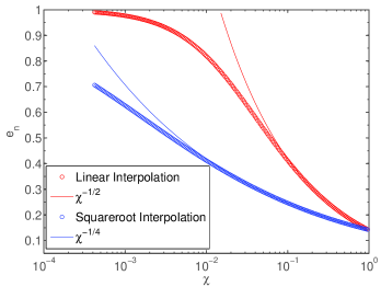
Figure 14: Semi-log plot of the coefficient of restitution as function of the scaled initial velocity $\chi$, using different interpolation rules for $k_{2}$, for pair collisions with $\eta=50$ and $\beta=0$. The symbols denote the solutions of the general equation, Eq. (C.2) with linear interpolation (red circles) or square root interpolation (blue circles), as given in Eq. (D.1). The red and blue solid lines represent the approximations for high impact velocity $e_{n}\sim\chi^{-1/2}$ and $e_{n}\sim\chi^{-1/4}$.

Appendix E Energy Picture

This appendix shows the energies of two particles during contact, where the difference between the different branches of the contact model, namely irreversible/unstable or reversible/elastic, will be highlighted.

   

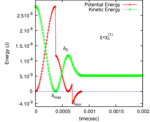
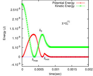
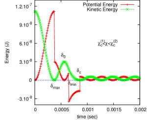
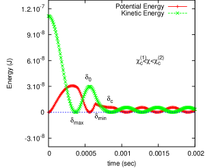
Figure 15: (a), (c) Kinetic and (irreversible, plastic, “potential”) energy of the particles, and (b), (d) kinetic and available (elastic) potential energy (for re-loading) of the particles, plotted against time for pair collisions with $k_{1}=10^{2}$ Nm^-1. $k_{p}=5\times 10^{2}$ Nm^-1, and $k_{c}=10^{2}$ Nm^-1, i.e. $\eta=4$ and $\beta=1$. The initial velocity $\chi$ is $\chi=0.34$ (a,b) and $\chi=0.69$ (c,d), in the regimes defined in the inset of each plot.

In Fig. 15, the time-evolution of kinetic and potential energy is shown; the graphs can be viewed in parallel to Figs. 7(a) and 7(b). In Fig. 15(a), we plot the kinetic and potential energy of the particles against time for low initial velocity $\chi<\chi^{(1)}_{c}$, corresponding to Fig. 7(a), for which dissipation is so weak that particles do not stick. The kinetic energy decreases from its initial value and is converted to potential energy (the conversion is complete at $\delta_{\rm max}$). Thereafter, the potential energy drops due to the change between the loading and unloading slope from $k_{1}$ to $k_{2}$. The potential energy decreases to zero (at the force-free overlap $\delta_{\rm 0}$), where it is converted to (less) kinetic energy. Then the kinetic energy decreases further due to the acting adhesive force. At $\delta_{\rm min}$ the increasing potential energy drops to a negative value due to the change in unloading slope from $k_{2}$ to the adhesive (instable) slope $-k_{c}$. From there it increases from this minimum, negative value to zero, for $\delta=0$. From here the kinetic energy remains constant and the potential energy stays at zero, since the particles are separated.

In Fig. 15(b), we plot the time evolution of kinetic and potential energy that the particles would have if un-/re-loading would take place at that moment, along the branch with slope $k_{2}$, namely the available (elastic) potential energy. This energy increases from zero at $t=0$, and reaches a maximum when the kinetic energy becomes zero (note that it is not equal to the initial kinetic energy due to the plastic change of slope of $k_{2}$.) Thereafter, the available potential energy decreases to zero at the force-free overlap $\delta_{\rm 0}$. For further unloading, the available potential energy first increases and then drops rapidly on the unstable branch with slope $-k_{c}$. The change in sign of the unloading slope, from $k_{2}$ to $-k_{c}$, is reflected in the kink in the curve at $\delta_{\rm min}$. Note, that comparing Figs. 15 and 15, the available potential energy always stays positive, while the total, plastic “potential” energy drops to negative values after the kink at $\delta_{\rm min}$.

Figs. 15(c) and 15(d) show the time evolution of kinetic and potential energy (total and available, respectively) for an initial velocity $\chi^{(1)}_{c}<\chi<\chi^{(2)}_{c}$ in the sticking regime, see Fig. 7(b). In Fig. 15(c), a similar trend as that of Fig. 15(a) is observed until the potential energy becomes negative at $\delta_{\rm min}$. The difference to the case of smaller impact velocity is that at this point, the kinetic energy is less than the magnitude of the negative potential energy and hence first reaches zero, i.e., the particles stick. At this point, the (plastic) potential energy increases and jumps to a positive value indicating the change in sign of the unloading slope from $-k_{c}$ to $k_{2}$. Finally, it oscillates between this positive value at $\delta_{\rm c}$, exchanging energy with the kinetic degree of freedom. When the available potential energy is plotted in Fig. 15(d), a similar trend as that of Fig. 15(b) is observed up to the kink at $\delta_{\rm min}$. Here, the two energies have comparable values when they reach $\delta_{\rm min}$ and the kinetic energy decreases to zero with a non-zero available potential energy, which causes the contact to re- and un-load along $k_{2}$.

Appendix F Cyclic agglomerate compression and tension tests

Goal of this appendix is to show the unloading and re-loading behavior of an agglomerate, i.e. its effective, mesoscopic force-displacement relation, which clearly is different from the contact force law applied at the primary particle contacts. We will report incomplete detachment and partly/weaker elastic response for re-loading after various different compressive and tensile loading amplitudes.

The system considered here is an agglomerate (cubic) of size $L_{0}=0.115$, made of $N=1728$ primary particles of diameter $d_{0}=0.01$ (with some variation in size to avoid monodisperse artefacts), just as in Ref. [15]. The cubic sample was first compressed (pressure-sintered) with a dimensionless wall stress $d_{0}p_{s}/k_{p}=0.02$ to form a stable, rather dense agglomerate or “tablet”. The stress is first released to a value $2.10^{-5}$, i.e. $p_{r}/p_{s}=10^{-3}$ for all walls. Then various uni-axial, unconfined tension/compression tests are carried out applying either further tension or compression starting from the released state of the sample [15]. The simulation parameters are same as in Ref. [15] (table 2), except for the cohesion that is set here to a rather small intensity, $k_{c}/k_{p}=0.2$, rolling and sliding friction coefficients that are double as large, $\mu_{r}=\mu_{o}=0.2$, and viscous damping of those degrees of freedom, $\gamma_{r}/\gamma=\gamma_{o}/\gamma=0.1$, which also is larger than that of the reference situation.

The force-displacement curves for the tests at different amplitudes are shown in Figs. 16 and 18 for tension and compression tests respectively. All simulations in Figs. 16 and 18 start from the same configuration, i.e. the released state mentioned above and is indicated by the black circle at point $(0,0)$. These plots represent the mesoscopic contact model of agglomerates consisting of multiple primary particles and their geometrical surface configurations and change in shape during the tests.

Fig. 16 shows the force-displacement curve for an unconfined uniaxial tension test. The black arrow shows the unloading/tension path, and finally arrows with different colors show the re-loading paths for different deformation amplitudes, as given in the inset. Each of the tests, when it reaches the original strain at zero, is then repeated for three more cycles. Note that repeated cyclic loading remains on the same branch with positive slope, displaying the elastic nature of the contact, while it is not completely, perfectly detached. The contact surface is changing plastically by restructuring of the primary particles and surely is not flat, see Fig. 17, as one would expect for ideal, homogeneous, plastic materials. For the largest amplitude, the behavior is not perfectly elastic anymore, since the first plastic effects show up. For deformations as large as 0.2 of the primary particle diameter, $d_{0}$, before re-loading (arrow with positive slope on the red curve) has mostly, but not completely lost mechanical contact. The complete detachment of the assembly happens for much higher amplitude, than what is expected from a two-particle interaction. Note that the contact model of the primary particles is behaving elasto-plastically $(\phi_{f}=0.05)$ on the scale of only $0.05d_{0}$; the reversible, elastic un-/re-loading is thus not due to the primary particle contact model, since it stretches to four times $\phi_{f}d_{0}$ and even higher displacements. Finally, in order to confirm that this is not an effect of viscosity, qualitatively, the thick lines are simulations performed four times slower than those with thin lines.

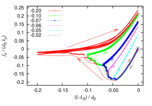
Figure 16: Dimensionless force-displacement curve for an unconfined uni-axial tension test (negative horizontal axis), with the various different deformation amplitudes $D_{x}$ given in the inset. The downward arrow indicates the direction of first tensile unloading, while the upwards-right arrows indicate the change of force during re-loading. Except for the red curve, all these branches are reversible, for repeated un-/re-loading.

Figure 17: Snapshots of the tablet-sample during (large) tensile deformations for $D_{x}=(L-L_{0})/d_{0}=0$ (a), 0.81 (b), 1.8 (c), 3.1 (d), 4.7 (e), 7.4 (f), and 8.6 (g). The primary particles are colored according to their distance from the viewer (red, green, blue is increasing distance).

In Fig. 17, a few snapshots during the tensile deformation are presented. The first snapshot corresponds to the undisturbed sample, while the others are increasing tensile deformation amplitudes. Note that these deformations are much larger than in Fig. 16. The contact is completely lost only at the extreme, final deformation in Fig. 19(g). In Fig. 17, it is also visible that the contact surface has developed a roughness of the size of several primary particles; the first visible gap is opened at a total deformation of $D_{x}\sim d_{0}$, and the contact is lost only at $D_{x}\sim 8d_{0}$, when the last of the thin “threads” breaks. The elastic, irreversible tension branch, however, is strongly developed only for much smaller $D_{x}\sim d_{0}/5$.

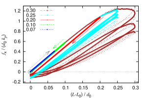
Figure 18: Dimensionless force-displacement curve for the same sample as in Fig. 16, but under compressive initial loading and un-/re-loading. The values in the inset indicate the maximal amplitudes $D_{x}$.

Complementing the tension test above, Fig. 18 shows the behavior of the same sample during compression cycles. The values given in the inset indicate the amplitude of un-/re-loading. The smallest amplitudes remain elastic throughout, while plastic deformation kicks in for $D_{x}>0.1$ (see the red curve). However, the unloading and re-loading take place on the same branch, i.e. a new elastic branch (e.g. for $D_{x}=0.2$). For even larger amplitudes, e.g. the yellow curve with $D_{x}=0.3$, the continuous damage/plastic destruction of the sample (by considerable irreversible re-arrangement during each cycle). Again, thick lines indicate simulations four times slower, which shows a small quantitative difference, but qualitative agreement even for the largest amplitude/rate. The snapshots in Fig. 19 show the continuous plastic deformation of the sample at large strains.

Figure 19: Snapshots of the tablet sample during compression at (large) deformations $D_{x}=(L-L_{0})/d_{0}=0$ (a), 0.01 (b), 0.3 (c), 0.8 (d), and 1.8 (e). The color code is small stress (green) and compressive/tensile larger stress (red/blue) averaged/isotropically per primary particle.

References

- [1] M. Paulick, M. Morgeneyer, and A. Kwade, “A new method for the determination of particle contact stiffness,” Granular Matter, vol. 17, no. 1, pp. 83–93, 2015.
- [2] T. Van Steenkiste, J. Smith, R. Teets, J. Moleski, D. Gorkiewicz, R. Tison, D. Marantz, K. Kowalsky, W. Riggs, P. Zajchowski, et al., “Kinetic spray coatings,” Surface and Coatings Technology, vol. 111, no. 1, pp. 62–71, 1999.
- [3] D. Zhang, P. Shipway, and D. McCartney, “Cold gas dynamic spraying of aluminum: The role of substrate characteristics in deposit formation,” Journal of Thermal Spray Technology, vol. 14, pp. 109–116, 2005.
- [4] T. Schmidt, F. Gärtner, H. Assadi, and H. Kreye, “Development of a generalized parameter window for cold spray deposition,” Acta Materialia, vol. 54, no. 3, pp. 729–742, 2006.
- [5] J. Wu, H. Fang, S. Yoon, H. Kim, and C. Lee, “The rebound phenomenon in kinetic spraying deposition,” Scripta Materialia, vol. 54, no. 4, pp. 665–669, 2006.
- [6] X. Zhou, X. Wu, J. Wang, J. Zhang, et al., “Numerical investigation of the rebounding and the deposition behavior of particles during cold spraying,” Acta Merall. Sin.(English Lett.), vol. 24, no. 1, pp. 45–53, 2011.
- [7] P. A. Cundall and O. D. L. Strack, “A discrete numerical model for granular assemblies,” Géotechnique, vol. 29, no. 1, pp. 47–65, 1979.
- [8] Y. M. Bashir and J. D. Goddard, “A novel simulation method for the quasi-static mechanics of granular assemblages,” Journal of Rheology, vol. 35, no. 5, pp. 849–885, 1991.
- [9] H. J. Herrmann, J.-P. Hovi, and S. Luding, eds., Physics of dry granular media - NATO ASI Series E 350, (Dordrecht), Kluwer Academic Publishers, 1998.
- [10] C. Thornton, “Numerical simulations of deviatoric shear deformation of granular media,” Géotechnique, vol. 50, no. 1, pp. 43–53, 2000.
- [11] C. Thornton and L. Zhang, “A DEM comparison of different shear testing devices,” in Powders & Grains 2001 (Y. Kishino, ed.), (Rotterdam), pp. 183–190, Balkema, 2001.
- [12] P. A. Vermeer, S. Diebels, W. Ehlers, H. J. Herrmann, S. Luding, and E. Ramm, eds., Continuous and Discontinuous Modelling of Cohesive Frictional Materials, (Berlin), Springer, 2001. Lecture Notes in Physics 568.
- [13] M. Lätzel, S. Luding, H. J. Herrmann, D. W. Howell, and R. P. Behringer, “Comparing simulation and experiment of a 2d granular couette shear device,” The European Physical Journal E, vol. 11, no. 4, pp. 325–333, 2003.
- [14] S. Luding, “Particulate solids modeling with discrete element methods,” in CHoPS-05 CD Proceedings (P. Massaci, G. Bonifazi, and S. Serranti, eds.), (Tel Aviv), pp. 1–10, ORTRA, 2006.
- [15] S. Luding, “Cohesive, frictional powders: contact models for tension,” Granular Matter, vol. 10, pp. 235–246, 2008.
- [16] K. L. Johnson, K. Kendall, and A. D. Roberts, “Surface energy and the contact of elastic solids,” Proceedings of Royal Society London A, vol. 324, no. 1558, pp. 301–313, 1971.
- [17] B. Derjaguin, V. Muller, and Y. P. Toporov, “Effect of contact deformations on the adhesion of particles,” Journal of Colloid and interface science, vol. 53, no. 2, pp. 314–326, 1975.
- [18] O. Molerus, “Theory of yield of cohesive powders,” Powder Technology, vol. 12, no. 3, pp. 259–275, 1975.
- [19] O. Molerus, “Effect of interparticle cohesive forces on the flow behaviour of powders,” Powder Technology, vol. 20, pp. 161–175, 1978.
- [20] C. Thornton and K. K. Yin, “Impact of elastic spheres with and without adhesion,” Powder Technol., vol. 65, p. 153, 1991.
- [21] C. Thornton and Z. Ning, “A theoretical model for the stick/bounce behaviour of adhesive, elastic-plastic spheres,” Powder technology, vol. 99, no. 2, pp. 154–162, 1998.
- [22] J. Tomas, “Particle adhesion fundamentals and bulk powder consolidation,” KONA Powder and Particle Journal, vol. 18, pp. 157–169, 2000.
- [23] J. Tomas, “Assessment of mechanical properties of cohesive particulate solids. part 1: Particle contact constitutive model,” Particulate Science and Technology: An International Journal, vol. 19, pp. 95–110, 2001.
- [24] J. Tomas, “Assessment of mechanical properties of cohesive particulate solids. part 2: Powder flow criteria,” Particulate Science and Technology: An International Journal, vol. 19, pp. 111–129, 2001.
- [25] S. Luding, K. Manetsberger, and J. Müllers, “A discrete model for long time sintering,” Journal of the Mechanics and Physics of Solids, vol. 53, no. 2, pp. 455–491, 2005.
- [26] C. Dominik and A. Tielens, “The physics of dust coagulation and the structure of dust aggregates in space,” The Astrophysical Journal, vol. 480, no. 2, p. 647, 1997.
- [27] G. S. Boltachev, N. Volkov, E. Dvilis, and O. Khasanov, “Compaction and elastic unloading of nanopowders in terms of granular dynamics,” Technical Physics, vol. 60, no. 2, pp. 252–259, 2015.
- [28] S. Luding and F. Alonso-Marroquín, “The critical-state yield stress (termination locus) of adhesive powders from a single numerical experiment,” Granular Matter, vol. 13, pp. 109–119, 2011.
- [29] A. Singh, V. Magnanimo, K. Saitoh, and S. Luding, “Effect of cohesion on shear banding in quasistatic granular materials,” Physical Review E, vol. 90, p. 022202, 2014.
- [30] A. Singh, Micro-macro and rheology in sheared granular matter. Universiteit Twente, 2014.
- [31] A. Singh, V. Magnanimo, K. Saitoh, and S. Luding, “The role of gravity or pressure and contact stiffness in granular rheology,” New Journal of Physics, vol. 17, no. 4, p. 043028, 2015.
- [32] A. Singh, V. Magnanimo, and S. Luding, “Effect of friction and cohesion on anisotropy in quasi-static granular materials under shear,” in AIP Conference Proceedings, vol. 1542, pp. 682–685, 2013.
- [33] S. Roy, A. Singh, S. Luding, and T. Weinhart, “Micro–macro transition and simplified contact models for wet granular materials,” Computational Particle Mechanics, pp. 1–14, 2015.
- [34] N. Kumar and S. Luding, “Memory of jamming–multiscale flow in soft and granular matter,” arXiv preprint arXiv:1407.6167, vol. 17.
- [35] E. Rojas, M. Trulsson, B. Andreotti, E. Clément, and R. Soto, “Relaxation processes after instantaneous shear-rate reversal in a dense granular flow,” EPL (Europhysics Letters), vol. 109, no. 6, p. 64002, 2015.
- [36] M. Jiang, Y. Sun, L. Li, and H. Zhu, “Contact behavior of idealized granules bonded in two different interparticle distances: An experimental investigation,” Mechanics of Materials, vol. 55, pp. 1 – 15, 2012.
- [37] M. Jiang, W. Zhang, Y. Sun, and S. Utili, “An investigation on loose cemented granular materials via dem analyses,” Granular Matter, vol. 15, no. 1, pp. 65–84, 2013.
- [38] L. Kempton, D. Pinson, S. Chew, P. Zulli, and A. Yu, “Simulation of macroscopic deformation using a sub-particle DEM approach,” Powder Technology, vol. 223, pp. 19 – 26, 2012.
- [39] O. Walton, “Potential discrete element simulation applications ranging from airborne fines to pellet beds,” in International Conference On Environmental Systems, vol. 01, p. 2329, 2004.
- [40] O. R. Walton and S. M. Johnson, “Simulating the effects of interparticle cohesion in micron-scale powders,” AIP Conference Proceedings, vol. 1145, no. 1, pp. 897–900, 2009.
- [41] S. C. Thakur, H. Ahmadian, J. Sun, and J. Y. Ooi, “An experimental and numerical study of packing, compression, and caking behaviour of detergent powders,” Particuology, vol. 12, pp. 2–12, 2014.
- [42] M. Pasha, S. Dogbe, C. Hare, A. Hassanpour, and M. Ghadiri, “A linear model of elasto-plastic and adhesive contact deformation,” Granular Matter, vol. 16, no. 1, pp. 151–162, 2014.
- [43] S. Thakur, J. Ooi, and H. Ahmadian, “Scaling of discrete element model parameter in uniaxial test simulation,” in The 6th International conference on discrete element methods,Golden, Colorado, USA., 2013.
- [44] Y. Rozenblat, A. Levy, H. Kalman, and J. Tomas, “Impact velocity and compression force relationship—equivalence function,” Powder Technology, vol. 235, pp. 756–763, 2013.
- [45] K. L. Johnson, Contact Mechanics. Cambridge: Cambridge Univ. Press, 1985.
- [46] G. Kuwabara and K. Kono, “Restitution coefficient in a collision between two spheres,” Japanese Journal of Applied Physics, vol. 26, no. 8, pp. 1230–1233, 1987.
- [47] O. R. Walton and R. L. Braun, “Stress calculations for assemblies of inelastic spheres in uniform shear,” Acta Mechanica, vol. 63, p. 73, 1986.
- [48] S. Luding, E. Clément, A. Blumen, J. Rajchenbach, and J. Duran, “Anomalous energy dissipation in molecular dynamics simulations of grains: The “detachment effect”,” Physical Review E, vol. 50, p. 4113, 1994.
- [49] N. V. Brilliantov, F. Spahn, J. M. Hertzsch, and T. Pöschel, “Model for collisions in granular gases,” Physical Review E, vol. 53, no. 5, p. 5382, 1996.
- [50] S. Luding, “Collisions & contacts between two particles,” in Physics of dry granular media - NATO ASI Series E350 (H. J. Herrmann, J.-P. Hovi, and S. Luding, eds.), (Dordrecht), p. 285, Kluwer Academic Publishers, 1998.
- [51] X. Zhang and L. Vu-Quoc, “Modeling the dependence of the coefficient of restitution on the impact velocity in elasto-plastic collisions,” International Journal of Impact Engineering, vol. 27, no. 3, pp. 317–341, 2002.
- [52] B. Dahneke, “Measurements of bouncing of small latex spheres,” Journal of Colloid and Interface Science, vol. 45, no. 3, pp. 584 – 590, 1973.
- [53] B. Dahneke, “Further measurements of the bouncing of small latex spheres,” Journal of Colloid and Interface Science, vol. 51, no. 1, pp. 58 – 65, 1975.
- [54] S. Wall, W. John, H.-C. Wang, and S. L. Goren, “Measurements of kinetic energy loss for particles impacting surfaces,” Aerosol Science and Technology, vol. 12, no. 4, pp. 926–946, 1990.
- [55] N. V. Brilliantov, N. Albers, F. Spahn, and T. Pöschel, “Collision dynamics of granular particles with adhesion,” Physical Review E, vol. 76, p. 051302, 2007.
- [56] C. Sorace, M. Louge, M. Crozier, and V. Law, “High apparent adhesion energy in the breakdown of normal restitution for binary impacts of small spheres at low speed,” Mechanics Research Communications, vol. 36, no. 3, pp. 364 – 368, 2009.
- [57] S. Li, J. S. Marshall, G. Liu, and Q. Yao, “Adhesive particulate flow: The discrete-element method and its application in energy and environmental engineering,” Progress in Energy and Combustion Science, vol. 37, no. 6, pp. 633 – 668, 2011.
- [58] D. A. Hanaor, Y. Gan, and I. Einav, “Contact mechanics of fractal surfaces by spline assisted discretisation,” International Journal of Solids and Structures, vol. 59, pp. 121–131, 2015.
- [59] K. Saitoh, A. Bodrova, H. Hayakawa, and N. V. Brilliantov, “Negative normal restitution coefficient found in simulation of nanocluster collisions,” Physical Review Letter, vol. 105, p. 238001, 2010.
- [60] P. Müller, D. Krengel, and T. Pöschel, “Negative coefficient of normal restitution,” Physical Review E, vol. 85, p. 041306, 2012.
- [61] R. Jasevičius, R. Kačianauskas, and J. Tomas, “Simulation of normal impact of micron-sized particle with elastic-plastic contact,” Journal of Vibroengineering, vol. 11, no. 1, pp. 6–16, 2009.
- [62] R. Jasevičius, J. Tomas, and R. Kačianauskas, “Simulation of normal impact of ultrafine silica particle on substrate,” Particulate Science and Technology, vol. 29, no. 2, pp. 107–126, 2011.
- [63] J. Tomas, “Adhesion of ultrafine particles – a micromechanical approach,” Chemical Engineering Science, vol. 62, no. 7, pp. 1997 – 2010, 2007.
- [64] T. Siu, W. Pittman, J. Cotton, and T. Shinbrot, “Nonlinear granular electrostatics,” Granular Matter, pp. 1–11, 2015.
- [65] D. Rathbone, M. Marigo, D. Dini, and B. van Wachem, “An accurate force–displacement law for the modelling of elastic–plastic contacts in discrete element simulations,” Powder Technology, 2015.
- [66] S. Herminghaus, “Dynamics of wet granular matter,” Advances in Physics, vol. 54, no. 3, pp. 221–261, 2005.
- [67] L. Brendel, J. Török, R. Kirsch, and U. Bröckel, “A contact model for the yielding of caked granular materials,” Granular Matter, vol. 13, no. 6, pp. 777–786, 2011.
- [68] C. Thornton, S. J. Cummins, and P. W. Cleary, “An investigation of the comparative behaviour of alternative contact force models during elastic collisions,” Powder Technology, vol. 210, no. 3, pp. 189 – 197, 2011.
- [69] C. Thornton, S. J. Cummins, and P. W. Cleary, “An investigation of the comparative behaviour of alternative contact force models during inelastic collisions,” Powder Technology, vol. 233, no. 0, pp. 30 – 46, 2013.
- [70] O. Walton, “Review of adhesion fundamentals for micron-scale particles,” KONA Powder and Particle Journal Powder and Particle, vol. 26, pp. 129–141, 2008.
- [71] O. R. Walton and R. L. Braun, “Viscosity, granular-temperature, and stress calculations for shearing assemblies of inelastic, frictional disks,” J. Rheol., vol. 30, no. 5, pp. 949–980, 1986.
- [72] D. S. Nasato, C. Goniva, S. Pirker, and C. Kloss, “Coarse graining for large-scale dem simulations of particle flow–an investigation on contact and cohesion models,” Procedia Engineering, vol. 102, pp. 1484–1490, 2015.
- [73] S. C. Thakur, J. Sun, J. Y. Ooi, and H. Ahmadian, “An experimental and numerical study of compression and shear behaviour of detergent powders,” in 7th International Conference on Conveying and Handling of Particulate Solids, 2012.
- [74] O. R. Walton, “Numerical simulation of inelastic, frictional particle-particle interactions,” in Particulate two-phase flow (M. C. Roco, ed.), (Boston), p. 884, Butterworth-Heinemann, 1993.
- [75] N. V. Brilliantov and T. Pöschel, Collision of Adhesive Viscoelastic Particles. Wiley VCH, 2005.
- [76] G. Haiat, M. P. Huy, and E. Barthel, “The adhesive contact of viscoelastic spheres,” Journal of the Mechanics and Physics of Solids, vol. 51, no. 1, pp. 69 – 99, 2003.
- [77] B. Dahneke, “The influence of flattening on the adhesion of particles,” Journal of Colloid and Interface Science, vol. 40, no. 1, pp. 1 – 13, 1972.
- [78] S. Luding and H. Herrmann, “Micro-macro transition for cohesive granular media,” Zur Beschreibung komplexen Materialverhaltens, Institut für Mechanik, S. Diebels (Ed.), Stuttgart, pp. 121–133, 2001.
- [79] H. Tanaka, K. Wada, T. Suyama, and S. Okuzumi, “Growth of cosmic dust aggregates and reexamination of particle interaction models,” Progress of Theoretical Physics Supplement, vol. 195, pp. 101–113, 2012.
- [80] M. P. Allen and D. J. Tildesley, Computer Simulation of Liquids. Oxford: Oxford University Press, 1987.
- [81] D. C. Rapaport, The Art of Molecular Dynamics Simulation. Cambridge: Cambridge University Press, 1995.
- [82] T. Pöschel and T. Schwager, Computational Granular Dynamics. Berlin: Springer, 2005.
- [83] V. Ogarko and S. Luding, “A fast multilevel algorithm for contact detection of arbitrarily polydisperse objects,” Computer physics communications, vol. 183, no. 4, pp. 931–936, 2012.
- [84] D. Krijgsman, V. Ogarko, and S. Luding, “Optimal parameters for a hierarchical grid data structure for contact detection in arbitrarily polydisperse particle systems,” Computational Particle Mechanics, vol. 1, no. 3, pp. 357–372, 2014.
- [85] L. Vu-Quoc and X. Zhang, “An elastic contact force-displacement model in the normal direction: displacement-driven version,” Proceedings Royal Society London A, vol. 455, pp. 4013–4044, 1999.
- [86] X. Zhang and L. Vu-Quoc, “Simulation of chute flow of soybeans using an improved tangential force-displacement model,” Mechanics of Materials, vol. 32, pp. 115–129, 2000.
- [87] A.-S. Persson and G. Frenning, “An experimental evaluation of the accuracy to simulate granule bed compression using the discrete element method,” Powder Technology, vol. 219, pp. 249 – 256, 2012.
- [88] T. Ormel, V. Magnanimo, H. t. Huerne, and S. Luding, “Modeling of asphalt and experiments with a discrete particles method,” in Conference Proceedings MAIREPAV7 2012, 2012.
- [89] A. Moridi, S. Hassani-Gangaraj, and M. Guagliano, “A hybrid approach to determine critical and erosion velocities in the cold spray process,” Applied Surface Science, vol. 273, pp. 617–624, 2013.
- [90] S. Luding, “From discrete particles to solids-about sintering and self-healing,” Computer Methods in Materials Science, vol. 11, no. 1, pp. 53–63, 2011.
- [91] J. Tomas and S. Kleinschmidt, “Improvement of flowability of fine cohesive powders by flow additives,” Chemical Engineering and Technology, vol. 32, no. 10, pp. 1470–1483, 2009.
- [92] A. Singh, V. Magnanimo, and S. Luding, “Effect of friction on the force distribution in sheared granular materials,” Proc. of NUMGE2014, pp. 409–14, 2014.
- [93] P. Müller and J. Tomas, “Simulation and calibration of granules using the discrete element method,” Particuology, vol. 12, pp. 40–43, 2014.
- [94] K. Mader-Arndt, Z. Kutelova, and J. Tomas, “Microscopic particle contact adhesion models and macroscopic behavior of surface modified particles,” Particle Adhesion and Removal, pp. 105–155, 2015.
- [95] M.-K. Müller, “Long-range interactions in dilute granular systems.” PhD-thesis, 2008.
- [96] M.-K. Müller and S. Luding, “Homogeneous cooling with repulsive and attractive long-range potentials,” Mathematical Modelling of Natural Phenomena, vol. 6, no. 04, pp. 118–150, 2011.
- [97] S. Gonzalez, “An investigation into clustering and segregation in granular materials.” PhD-thesis, 2013.
- [98] S. Gonzalez, A. R. Thornton, and S. Luding, “Free cooling phase-diagram of hard-spheres with short- and long-range interactions,” Europ. Phys. J. - Special Topics, vol. 223(11), pp. 2205–2225, 2014.
- [99] S. Kothe, J. Blum, R. Weidling, and C. Güttler, “Free collisions in a microgravity many-particle experiment. III: The collision behavior of sub-millimeter-sized dust aggregates,” Icarus, vol. 225, no. 1, pp. 75–85, 2013.
- [100] O. I. Imole, D. Krijgsman, T. Weinhart, V. Magnanimo, B. E. C. Montes, M. Ramaioli, and S. Luding, “Experiments and discrete element simulation of the dosing of cohesive powders in a simplified geometry,” arXiv preprint arXiv:1410.2886, 2014.
- [101] S. Luding, E. Clément, A. Blumen, J. Rajchenbach, and J. Duran, “Interaction laws and the detachment effect in granular media,” in Fractal Aspects of Materials, vol. 367, (Pittsburgh, Pennsylvania), pp. 495–500, Materials Research Society, Symposium Proceedings, 1995.
- [102] A. P. Hatzes, F. Bridges, D. N. C. Lin, and S. Sachtjen, “Coagulation of particles in saturn’s rings: Measurements of the cohesive force of water frost,” Icarus, vol. 89, no. 1, pp. 113 – 121, 1991.