The Doubloon Models

Abstract

A family of spherical halo models with flat circular velocity curves is presented. This includes models in which the rotation curve has a finite central value but declines outwards (like the Jaffe model). It includes models in which the rotation curve is rising in the inner parts, but flattens asymptotically (like the Binney model). The family encompasses models with both finite and singular (cuspy) density profiles. The self-consistent distribution function depending on binding energy $E$ and angular momentum $L$ is derived and the kinematical properties of the models discussed. These really describe the properties of the total matter (both luminous and dark).

For comparison with observations, it is better to consider tracer populations of stars. These can be used to represent elliptical galaxies or the spheroidal components of spiral galaxies. Accordingly, we study the properties of tracers with power-law or Einasto profiles moving in the doubloon potential. Under the assumption of spherical alignment, we provide a simple way to solve the Jeans equations for the velocity dispersions. This choice of alignment is supported by observations on the stellar halo of the Milky Way. Power-law tracers have prolate spheroidal velocity ellipsoids everywhere. However, this is not the case for Einasto tracers, for which the velocity ellipsoids change from prolate to oblate spheroidal near the pole.

Asymptotic forms of the velocity distributions close to the escape speed are also derived, with an eye to application to the high velocity stars in the Milky Way. Power-law tracers have power-law or Maxwellian velocity distributions tails, whereas Einasto tracers have super-exponential cut-offs.

1 INTRODUCTION

The study of spherical models is useful both for representing galaxies and dark haloes. Even though flattening is often important, spherical models have provided useful insights into the behaviour of stellar systems. They can serve as starting points for more flattened models, either as initial conditions for N-Body experiments or as the lowest order terms in basis function expansions (Hernquist & Ostriker, 1992).

An important family of spherical models discovered over the last twenty-five years is the double-power law or $\gamma$ models (Dehnen, 1993; Tremaine et al., 1994). These have a density profile that is cusped like $r^{-\gamma}$ at small radii, yet falls like $r^{-4}$ at large radii. They have found ready applications in modern astronomy. They include two particularly simple and appealing models found earlier by Jaffe (1983) and Hernquist (1990), which differ in the strength of the central density cusp, $\rho\sim r^{-2}$ and $r^{-1}$ respectively. All the double-power law models generate simple gravitational potentials or force-laws. They also have analytically tractable distribution functions (DFs). This is technically challenging, as an integral equation has to be solved (see e.g., Eddington, 1916; Binney & Tremaine, 2008). Nonetheless, DFs are useful as they encode all the properties of the model, enabling initial conditions to be set for N-body realisations of distributions of observables to be computed.

Here, we provide another very simple family of spherical double-power law halo models – the doubloon models. They are motivated by the flatness of galaxy rotation curves, and so the models have a density that falls like $r^{-2}$, either in the inner parts or the outer parts. This generates a regime in which the rotation curve is roughly flattish. Explicitly, we consider the potential-density pair

$$\psi=-{V^{2}\over p}\log\biggl{(}{r^{p}+a^{p}\over a^{p}}\biggr{)},\quad\rho={V^{2}\over 4\pi Gr^{2-p}}{(1+p)\,a^{p}+r^{p}\over(a^{p}+r^{p})^{2}}.$$ (1)

Then, the rotation curve of the model is

$$v_{\rm c}(r)=V\biggl{(}1+{a^{p}\over r^{p}}\biggr{)}^{-1/2}.$$ (2)

Here, $V$ is the amplitude of the flat rotation curve, whilst $a$ is a scalelength. The density is positive everywhere provided $p\geq-1$, whereas it is monotonically decreasing (and hence astrophysically realistic) provided $p\leq 2$. When $p=0$, the model degenerates into the singular isothermal sphere (i.e. $\rho\propto r^{-2}$ but the strict limit is scaled to $v_{\rm c}=V/\sqrt{2}$), known for over a century thanks to the labours of J. H. Lane and R. Emden (see also Chandrasekhar, 1939).

The properties of the family divide neatly into two, as shown by their central and asymptotic behaviour. If $p>0$, the density falls off like $r^{-2}$ as $r\to\infty$ and the rotation curve is flat asymptotically

$$v_{\rm c}(r)\simeq V\times\begin{cases}(r/a)^{p/2}&(r\ll a)\\ 1&(r\gg a)\end{cases},$$ (3)

which we shall subsequently refer to the outer branch. The potential of the outer branch decreases from $\psi(0)=0$ to $\psi(\infty)=-\infty$ as $r$ increases, and the models possess the central density cusp like $1/r^{2-p}$ (except for $p=2$). Some of the usual suspects are represented in the family. When $p=2$, the model is the spherical limit of Binney’s logarithmic potential (Binney, 1981; Evans, 1993; Binney & Tremaine, 2008). When $p=1$, the model has a $1/r$ cusp and has recently been discussed by Evans & Williams (2014).

The rotation curve for models with $p<0$ tends to a finite value at the centre

$$v_{\rm c}(r)\simeq V\times\begin{cases}1&(r\ll a)\\ (a/r)^{|p|/2}&(r\gg a)\end{cases},$$ (4)

but falls off like $r^{-|p|/2}$ as $r\to\infty$. Henceforth these models will be referred to as the inner branch. The density always has an isothermal cusp ($\sim r^{-2}$) at the centre and decays like $r^{-(2+|p|)}$ as $r\to\infty$ (with the exception of the case $p=-1$), whereas the potential runs from $\psi(0)=\infty$ to $\psi(\infty)=0$. The model with $p=-1$ and was introduced by Jaffe (1983) as a representation of elliptical galaxies and has finite mass ($M=aV^{2}/G$). The remaining members of the family have rotation curves which fall off less steeply than the Jaffe model.

Both branches of the doubloon family are useful. For example, models on the inner branch are helpful in studies of the outer parts of galaxies, when the flat rotation curve gives out and the density of the dark matter begins to fade. Evidence, for example, from the Sagittarius stream suggests that the rotation curve of the Milky Way is flat out to $\sim 50~{}\mbox{kpc}$, and then begins to fall (Gibbons et al, 2014). Models on the outer branch are useful for studying the inner parts of galaxies, in the regime of the flat rotation curve. Their central cusps make them desirable models of dark matter haloes, in accord with predictions of dissipationless theories of galaxy formation (Mo, van den Bosch & White, 2010).

The paper is arranged as follows. Section 2 studies the self-consistent model, and gives families for the distribution functions for the total (dark and luminous) matter. These are self-consistent models and so are useful both for setting up the initial conditions for N-body experiments and for studying the kinematic properties of the dark and luminous matter. The remainder of the paper studies tracer populations moving in the doubloon potential. The tracers might represent stellar populations in elliptical galaxies or the spheroidal components of spiral galaxies. In particular, Section 3 looks at the Jeans solutions of tracer populations (with power-law or Einasto profiles), whilst Section 4 studies the distributions of high velocity stars. Both applications are motivated by the data on halo stars in the Milky Way, which has increased in quality and quantity in recent years thanks to surveys like SDSS and RAVE (see e.g., Smith et al., 2007, 2009a, 2009b; Bond et al., 2010; Piffl et al., 2014).

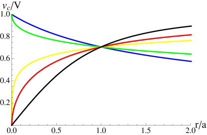
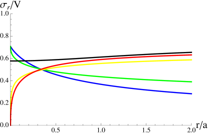
Figure 1: Rotation curves $v_{\rm c}$ (upper) and isotropic velocity dispersion $\sigma_{r}$ profiles (lower) for the models $p=2$ (black), $p=1$ (red), $p=1/2$ (yellow), $p=-1/2$ (green) and $p=-1$ (blue).

2 The Self Consistent Model

The phase space distribution function (DF) may depend on the integrals of motion only, as first realised by Jeans (1919). For a spherical potential, the integrals may be taken as the binding energy per unit mass $E$ and the modulus of the angular momentum $L$, namely

$$E=-\tfrac{1}{2}({v_{r}^{2}+v_{\theta}^{2}+v_{\phi}^{2}})+\psi,\quad L^{2}=r^{2}(v_{\theta}^{2}+v_{\phi}^{2}).$$ (5)

Isotropic DFs depend only on $E$, whereas anisotropic DFs depend on $L$ as well. Here we look for constant anisotropy DFs; that is, the anisotropy parameter $\beta\equiv 1-\langle v_{\theta}^{2}\rangle/\langle v_{r}^{2}\rangle$ takes a constant value. The parameter $\beta$ may take values in the range $-\infty\leq\beta\leq 1$. When $\beta\rightarrow 1$, the model is built from radial orbits, whilst when $\beta\rightarrow-\infty$, it is made from circular orbits. Constant anisotropy DFs are widely-used because of their simplicity. However, it is important to acknowledge that there is no underlying physical justification. Simulations of the growth of galaxies suggest that DFs are typically isotropic in the center ($\beta\approx 0$), but become more radially anisotropic ($\beta\approx 1/2$) in the outer parts (Hansen & Moore, 2006). It is nonetheless reasonable to expect that constant anisotropy DFs provide good approximations in certain regimes, such as the central parts or the outer periphery.

The velocity dispersions of the constant anisotropy models are found by integrating the Jeans equation, namely

$$\langle v_{r}^{2}\rangle=\frac{1}{r^{2\beta}\rho(r)}\int_{\infty}^{r}\!{\rm d}\tilde{r}\,\tilde{r}^{2\beta}\rho(\tilde{r})\,\frac{{\rm d}\psi}{{\rm d}r}\biggr{\rvert}_{r=\tilde{r}},$$ (6)

and $\langle v_{\theta}^{2}\rangle=(1-\beta)\langle v_{r}^{2}\rangle$. For the self-consistent doubloon models in equation (1) on the outer branch, assuming $0<p\leq 2(1-\beta)$,

$$\langle v_{r}^{2}\rangle={V^{2}r^{p}\over(1+p)\,a^{p}+r^{p}}\\ \times\left[{r^{2(1-\beta-p)}(a^{p}+r^{p})^{2}\over a^{2(1-\beta)}}(1+\lambda){\rm B}_{y}\bigl{(}1+\lambda,1-\lambda\bigr{)}-{1\over 2}\right],$$ (7)

where $\lambda\equiv 2p^{-1}(1-\beta)-1\geq 0$ and $y\equiv a^{p}/(a^{p}+r^{p})$, whilst ${\rm B}_{x}(a,b)$ is the incomplete beta function (Abramowitz & Stegun 1964, § 6.6; Olver et al. 2010, § 8.17). For all members, the velocity dispersion tends asymptotically to $\langle v_{r}^{2}\rangle^{1/2}\to V/\!\sqrt{2(1-\beta)}$ as $r\to\infty$. As $r\to 0$, it behaves like $\langle v_{r}^{2}\rangle\sim r^{\min(p,2-2\beta-p)}$, with the exception of the case $\beta=1-p$ when $\langle v_{r}^{2}\rangle\sim r^{p}\log r$. The radial velocity dispersion velocity tends to zero at the center, except for when $\beta=1-p/2$.

For the inner branch models ($-1\leq p<0$), we find

$$\langle v_{r}^{2}\rangle={V^{2}\over 1+(1-|p|)\,x}\left[\left({r\over a}\right)^{2(1-\beta)}(1+x)^{2}\xi{\rm B}_{1\over 1+x}\bigl{(}2+\xi,-\xi\bigr{)}-{1\over 2}\right],$$ (8)

where $\xi\equiv 2|p|^{-1}(1-\beta)=-1-\lambda\geq 0$ and $x\equiv(a/r)^{p}=(r/a)^{|p|}$. This is finite at the centre for $\beta<1$, as $\lim_{r\to 0}\langle v_{r}^{2}\rangle^{1/2}=V/\!\sqrt{2(1-\beta)}$, whilst it decays like $\langle v_{r}^{2}\rangle\simeq(V^{2}/2)(1-\beta+|p|)^{-1}(a/r)^{|p|}$ as $r\to\infty$. Plots of the isotropic ($\beta=0$) velocity dispersion are shown in Fig 1 as an illustration of some of these properties.

The key to the simplicity of the doubloon models is that $\psi(r)$ can be easily inverted, namely

$$r(\psi)=a\left[\exp\biggl{(}-{p\psi\over V^{2}}\biggr{)}-1\right]^{1/p}.$$ (9)

This means that $\rho(\psi)$ can also be easily constructed

$$\rho(\psi)={V^{2}\over 4\pi Ga^{2}}{{\rm e}^{2\psi/V^{2}}+p\,{\rm e}^{(p+2)\psi/V^{2}}\over\bigl{(}1-{\rm e}^{p\psi/V^{2}}\bigr{)}^{2/p-1}}.$$ (10)

From this, we can use Eddington’s (1916) formula to derive the isotropic DF via Abel transforms (see Binney & Tremaine, 2008). For anisotropic DFs, we similarly construct the augmented density

$$g(\psi)\equiv(2r^{2})^{\beta}\rho(\psi)={2^{\beta-2}V^{2}\over\pi Ga^{2(1-\beta)}}{{\rm e}^{p\psi/V^{2}}+p\,{\rm e}^{2p\psi/V^{2}}\over\bigl{(}{\rm e}^{-p\psi/V^{2}}-1\bigr{)}^{2(1-\beta)/p-1}}.$$ (11)

Then the constant anisotropy DF has the form of:

$$F(E,L)=\frac{f_{E}(E)\,H_{\beta}(L^{2})}{(2\pi)^{3/2}},\quad H_{\beta}(L^{2})\equiv\begin{cases}\dfrac{L^{-2\beta}}{\Gamma(1-\beta)}&(\beta<1)\\ \delta(L^{2})&(\beta=1)\end{cases},$$ (12)

where $\delta(x)$ is the Dirac delta function, whilst $g(\psi)$ at a fixed $\beta$ is given as an integral transformation of $f_{E}(E)$. The explicit relationship between $g(\psi)$ and $f_{E}(E)$ is found in the literature; e.g., Wilkinson & Evans (1999, eq. 2) or Evans & An (2006, eqs. 2 & 3). We outline a general algorithm to find $f_{E}(E)$ given $g(\psi)$ in Appendix A, which is an elaboration of Eddington’s inversion for isotropic DFs in terms of Abel transforms.

We note that the outer branch gives simpler DFs than the inner branch. For the outer branch, the DF is always a sum over isothermal or Maxwell–Boltzmann distributions. Usually, the sum is infinite, but, for some special cases, the sum is finite. For the inner branch, the DF is a sum over incomplete gamma functions (cf. Erdélyi et al. 1953, vol. 2, chap. IX; Abramowitz & Stegun 1964, § 6.5; Olver et al. 2010, chap. 8). Under some circumstances, the sum is finite and over Dawson’s integrals (which are equivalent to error functions). Although we give the general solutions, we point out some of the simple cases along the way.

2.1 Outer Branch

A physical model must have an everywhere positive DF. Since $\rho\sim r^{2-p}$ as $r\to 0$ for the self-consistent model with $p>0$, the cusp slope–central anisotropy theorem of An & Evans (2006a) indicates that the constant anisotropy DF is physical only if $2\beta\leq 2-p$. The constant anisotropy model for $p>0$ has the DF expressible as the sum over the exponentials of $p\bar{\mathcal{E}}$ where $\bar{\mathcal{E}}\equiv E/V^{2}$, namely

$$F=\frac{(1-\beta)^{3/2-\beta}}{4\pi^{5/2}\Gamma(1-\beta)}\frac{a^{2\beta-2}V^{2\beta-1}}{GL^{2\beta}}{\rm e}^{(1+\lambda)p\bar{\mathcal{E}}}\\ \times\Biggl{[}1+\sum_{j=1}^{\infty}\biggl{(}\frac{(\lambda-1)_{j}}{j!}+\frac{(1+p)(\lambda)_{j-1}}{(j-1)!}\biggr{)}\biggl{(}1+\frac{j}{1+\lambda}\biggr{)}^{\frac{3}{2}-\beta}{\rm e}^{jp\bar{\mathcal{E}}}\Biggr{]},$$ (13)

where $(\lambda)_{j}=\prod_{i=0}^{j-1}(\lambda+i)$ is the Pochhammer symbol and $\Gamma(x)$ is the gamma function. Also note $\lambda\equiv 2(1-\beta)/p-1\geq 0$. For $p=1$ (the halo model with the $1/r$ density cusp), this reduces to the expression given by Evans & Williams (2014). Experimentation shows that the sum over the exponentials converges rapidly, so this is a practical way to compute the DF.

There is a particularly simple case that is worthy of note. If $\lambda=0$ (i.e. $\beta=1-p/2$), then the DF reduces to just a sum over two isothermals, multiplied by a power of the angular momentum

$$F=\frac{V^{1-p}L^{p-2}}{4\pi^{5/2}\Gamma(p/2)\,Ga^{p}}\,\biggl{[}\left({p\over 2}\right)^{\frac{1+p}{2}}{\rm e}^{p\bar{\mathcal{E}}}+p^{\frac{3+p}{2}}{\rm e}^{2p\bar{\mathcal{E}}}\biggr{]}.$$ (14)

These are amongst the simplest DFs known, and some particular cases of this family have already appeared in the literature. So, for Binney’s logarithmic model ($p=2$),

$$F=\frac{1}{\pi^{5/2}Ga^{2}V}\Biggl{[}\frac{1}{4}\exp\biggl{(}\frac{2E}{V^{2}}\biggr{)}+\!\sqrt{2}\exp\biggl{(}\frac{4E}{V^{2}}\biggr{)}\Biggr{]},$$ (15)

which reduces to the isotropic DF comprised of two isothermals given in Evans (1993). For the halo model with the $1/r$ density cusp ($p=1$), it reduces to the simple anisotropic DF found in Evans & Williams (2014),

$$F=\frac{1}{\pi^{3}GaL}\Biggl{[}\frac{1}{8}\exp\biggl{(}\frac{E}{V^{2}}\biggr{)}+\frac{1}{4}\exp\biggl{(}\frac{2E}{V^{2}}\biggr{)}\Biggr{]}.$$ (16)

For all $p$, the velocity dispersions corresponding to the DF of equation (14) are analytic and given by:

$$\langle v_{r}^{2}\rangle={V^{2}\over 2p}{(2+p)\,a^{p}+2r^{p}\over(1+p)\,a^{p}+r^{p}},\quad\langle v_{\theta}^{2}\rangle={V^{2}\over 4}{(2+p)\,a^{p}+2r^{p}\over(1+p)\,a^{p}+r^{p}}.$$ (17)

This provides a simple solution to the Jeans equations for the velocity dispersions.

We remark that (i) the same simplicity occurs for the hypervirial models when the cusp slope $p$ and anisotropy $\beta$ are related $\beta=1-p/2$ (Evans & An, 2005) and that (ii) this combination of cusp slope and anisotropy is at the extreme permitted by the cusp slope-anisotropy theorem.

If $\lambda=1$ (i.e. $\beta=1-p$) on the other hand,

$$F=\frac{p^{1/2+p}V^{1-2p}L^{2(p-1)}}{4\pi^{5/2}\Gamma(p)\,Ga^{2p}}\biggl{(}{\rm e}^{2p\bar{\mathcal{E}}}+(1+p)\sum_{j=3}^{\infty}\left({j\over 2}\right)^{\frac{1}{2}+p}{\rm e}^{jp\bar{\mathcal{E}}}\biggr{)}.$$ (18)

with the velocity dispersions expressible analytically to be

$$\langle v_{r}^{2}\rangle={V^{2}r^{p}\over(1+p)\,a^{p}+r^{p}}\\ \times\left\{{1+p\over p}\Biggl{[}\biggl{(}1+{r^{p}\over a^{p}}\biggr{)}^{2}\log\biggl{(}1+{a^{p}\over r^{p}}\biggr{)}-{r^{p}\over a^{p}}\Biggr{]}-{2+3p\over 2p}\right\}.$$ (19)

Finally, we give the isotropic ($\beta=0$ and so $\lambda=2/p-1$) or ergodic DF that depends only on energy, which is, for $0<p\leq 2$

$$F={1\over 4\pi^{5/2}Ga^{2}V}\exp\biggl{(}\frac{2E}{V^{2}}\biggr{)}\,\\ \times\Biggl{[}1+\sum_{j=1}^{\infty}\biggl{(}\frac{({2\over p}-2)_{j}}{j!}+\frac{(1+p)({2\over p}-1)_{j-1}}{(j-1)!}\biggr{)}\biggl{(}1+{jp\over 2}\biggr{)}^{\frac{3}{2}}{\rm e}^{jp\bar{\mathcal{E}}}\Biggr{]}.$$ (20)

For $p=2$, this simplifies to equation (15), whilst if $p=1$, this reduces to

$$F={1\over 4\pi^{5/2}Ga^{2}V}\,\Biggl{[}\exp\biggl{(}\frac{2E}{V^{2}}\biggr{)}+(1+p)\sum_{j=3}^{\infty}\biggl{(}{j\over 2}\biggr{)}^{\frac{3}{2}}\exp\biggl{(}\frac{jE}{V^{2}}\biggr{)}\Biggr{]}.$$ (21)

The isotropic velocity dispersion resulting from the ergodic DF is

$$\langle v_{r}^{2}\rangle={V^{2}r^{p}\over(1+p)\,a^{p}+r^{p}}\left[{r^{2(1-p)}(a^{p}+r^{p})^{2}\over a^{2}}{2\over p}{\rm B}_{y}\biggl{(}\frac{2}{p},2-\frac{2}{p}\biggr{)}-{1\over 2}\right]$$ (22)

where $y\equiv a^{p}/(a^{p}+r^{p})$, with the particular cases of

$$\begin{split}\langle v_{r}^{2}\rangle&={V^{2}\over 2}{2a^{2}+r^{2}\over 3a^{2}+r^{2}}&(p=2),\\ \langle v_{r}^{2}\rangle&={V^{2}r\over 2a+r}\biggl{[}{2(a+r)^{2}\over a^{2}}\log\Bigl{(}1+{a\over r}\Bigr{)}-{5a+4r\over 2a}\biggr{]}&(p=1).\end{split}$$ (23)

As $r\to 0$, the velocity dispersion tends to zero (unless $p=2$, for which $\langle v_{r}^{2}\rangle\to V^{2}/3$), whilst it tends to $\langle v_{r}^{2}\rangle\to V^{2}/2$ as $r\to\infty$.

2.2 Inner Branch

The inner branches possesses more complicated DFs than the outer branch. This may be guessed from the properties of the Jaffe (1983) model, whose isotropic DF, first found by Jaffe and subsequently reported in Binney & Tremaine (2008), is already a sum of special functions (viz. Dawson’s integral).

Once we expand $g(\psi)$ in a power-series in ${\rm e}^{-|p|\psi/V^{2}}\leq 1$, the constant anisotropy DF in general is expressible as a sum over the incomplete gamma functions. The sum terminates after a finite number of terms if $2|p|^{-1}(1-\beta)$ is a non-negative integer. If $\beta$ is a half-integer, the actual operation reduces to ordinary derivatives (rather than Abel transforms or fractional derivatives) and so the result is eventually expressible by means of a rational function of exponentials. If $\beta$ is an integer, the resulting incomplete gamma functions are reducible to the error function (or equivalently Dawson’s integral). If $|p|=2(1-\beta)/n\leq 1$ where $n$ is a positive integer, the final expression is resolved into a finite sum over such functions, as is the case for the isotropic Jaffe model.

2.2.1 Models with radially biased orbit distributions

The simplest constant anisotropy DFs for the inner branch models are obtained for $\beta=1/2$. These models are of widespread physical applicability, as numerical simulations suggest that these are characteristic of dark matter haloes, at least in the outer parts (e.g., Hansen & Moore, 2006). Using the notation $\bar{\mathcal{E}}\equiv E/V^{2}$, we find:

$$F=\frac{\bigl{(}{\rm e}^{|p|\bar{\mathcal{E}}}-1\bigr{)}^{1/|p|}}{(2\pi)^{3}GaL}\left(1+|p|^{2}{\rm e}^{-|p|\bar{\mathcal{E}}}-2|p|^{2}{\rm e}^{-2|p|\bar{\mathcal{E}}}\right),$$ (24)

which therefore provides a simple radially anisotropic DF for all the doubloon models on the inner branch. For $p=-1$,

$$F=\frac{\exp(\bar{\mathcal{E}})-3\exp(-\bar{\mathcal{E}})+2\exp(-2\bar{\mathcal{E}})}{(2\pi)^{3}GaL},$$ (25)

which is the DF for the Jaffe sphere. This should be particularly useful in setting up initial conditions for N-body experiments.

All the models on the inner branch exhibit an isothermal cusp and so it is technically possible to set up the model composed entirely of radial orbits, although the resulting models will in general be prey to the radial orbit instability (Fridman & Polyachenko, 1984; Palmer & Papaloizou, 1987). The DFs of the radial orbit models are given in the closed form;

$$F=\frac{V\delta(L^{2})}{2^{3/2}\pi^{3}G}\biggl{[}\!\sqrt{|p|}\,(1+|p|)\,D_{+}\Bigl{(}\!\sqrt{|p|\bar{\mathcal{E}}}\Bigr{)}-\!\sqrt{2}|p|^{\frac{3}{2}}D_{+}\Bigl{(}\!\sqrt{2|p|\bar{\mathcal{E}}}\Bigr{)}\biggr{]},$$ (26)

utilizing Dawson’s integrals (see Binney & Tremaine, 2008, though here we use $D_{\pm}$ instead of $F_{\pm}$ to avoid confusion with the DF):

$$D_{\pm}(x)\equiv\exp(\mp x^{2})\int_{0}^{x}\exp(\pm t^{2})\,{\rm d}t.$$ (27)

This is actually closely related to the error function; that is, $D_{+}(x)=(\!\sqrt{\pi}/2){\rm e}^{-x^{2}}{\rm erfi}(x)$ and $D_{-}(x)=(\!\sqrt{\pi}/2){\rm e}^{x^{2}}{\rm erf}(x)$, where ${\rm erfi}(x)={\rm i}^{-1}{\rm erf}({\rm i}x)$ is the imaginary error function. The radial velocity dispersions corresponding to the pure radial orbit models are expressible using only elementary functions

$$\langle v_{r}^{2}\rangle={V^{2}\over|p|}{(1+x)^{2}\log(1+x^{-1})-x-1-|p|/2\over 1+(1-|p|)\,x},$$ (28)

where $x\equiv(a/r)^{p}=(r/a)^{|p|}$, which behaves like $\langle v_{r}^{2}\rangle\simeq V^{2}\log(a/r)$ as $r\to 0$ and $\langle v_{r}^{2}\rangle\simeq V^{2}(2|p|)^{-1}(a/r)^{|p|}$ as $r\to\infty$, respectively.

2.2.2 The Jaffe model

In fact, the Jaffe model deserves particular attention, as it is often used a model of a dark halo or an elliptical galaxy (see e.g., Kochanek, 1996; Gerhard et al., 1998). The radial velocity dispersion of the constant anisotropy Jaffe model is given by

$$\langle v_{r}^{2}\rangle=V^{2}{r^{2(1-\beta)}(a+r)^{2}\over a^{2(2-\beta)}}{\rm B}_{a\over a+r}\bigl{(}5-2\beta,2\beta-2\bigr{)},$$ (29a)

which is reducible to an elementary function if $$2\beta n=2-2\beta$$ is an integer – in particular, if is a non-negative integer,

$$\begin{split}\frac{\langle v_{r}^{2}\rangle}{V^{2}}={(1+n)(2+n)\over 2}\biggl{(}1+{r\over a}\biggr{)}^{2}\Phi_{n}\biggl{(}{r\over a}\biggr{)}-{3+n\over 2}-{2+n\over 2}{r\over a};\\ \Phi_{n}(x)=\sum_{k=1}^{\infty}{(-1)^{k-1}\over(n+k)x^{k}}=(-x)^{n}\biggl{[}\log\Bigl{(}1+{1\over x}\Bigr{)}+\sum_{k=1}^{n}{(-1)^{k}\over kx^{k}}\biggr{]}.\end{split}$$ (29b)

An analytic DF of the Jaffe model with $\beta=1/2$ is already provided in equation (25). Similar analytic DFs of the Jaffe model may also be obtained for all half-integer values of the anisotropy parameter. For instance, if $\beta=-1/2$,

$$F=\frac{\bigl{(}{\rm e}^{\bar{\mathcal{E}}}-1\bigr{)}^{3}\bigl{(}9+7{\rm e}^{-\bar{\mathcal{E}}}+4{\rm e}^{-2\bar{\mathcal{E}}}\bigr{)}\,L}{(2\pi)^{3}Ga^{3}V^{2}}.$$ (30)

For an integer value of the anisotropy parameter, the constant anisotropy DF of the Jaffe model is expressible as a finite sum over Dawson’s integrals. In particular, the DF with only radial orbits is

$$F=\frac{V\delta(L^{2})}{2\pi^{3}G}\left[\!\sqrt{2}\,D_{+}\Bigl{(}\!\sqrt{\bar{\mathcal{E}}}\Bigr{)}-D_{+}\Bigl{(}\!\sqrt{2\bar{\mathcal{E}}}\Bigr{)}\right],$$ (31)

whilst the Jaffe models with $-\beta=n\in\{0,1,\dotsc\}$:

$$F=\frac{a^{-2(1+n)}V^{-(1+2n)}L^{2n}}{2^{n+5/2}\pi^{3}n!G}\sum_{j=-2}^{2(n+1)}\frac{(-1)^{j}\!j^{n+2}}{|j|^{1/2}}{2n+4\choose j+2}\,D_{-({\rm sgn}\,j)}\Bigl{(}\!\sqrt{|j|\bar{\mathcal{E}}}\Bigr{)}\\ =\frac{a^{-2(1+n)}V^{-(1+2n)}L^{2n}}{2^{n+5/2}\pi^{5/2}n!G}\Biggl{[}\sum_{j=1}^{2(n+1)}\frac{(-1)^{j}\!j^{n+\frac{3}{2}}}{2}{2n+4\choose j+2}\,{\rm e}^{j\bar{\mathcal{E}}}{\rm erf}\bigl{(}\!\sqrt{j\bar{\mathcal{E}}}\bigr{)}\\ -(-1)^{n}(n+2){\rm e}^{-\bar{\mathcal{E}}}{\rm erfi}\bigl{(}\!\sqrt{\bar{\mathcal{E}}}\bigr{)}+(-2)^{n}\!\sqrt{2}{\rm e}^{-2\bar{\mathcal{E}}}{\rm erfi}\bigl{(}\!\sqrt{2\bar{\mathcal{E}}}\bigr{)}\Biggr{]}$$ (32)

where $D_{0}=0$ and ${a\choose n}$ is the binomial coefficient. The isotropic Jaffe model is included as the special case ($n=0$)

$$F={D_{+}\bigl{(}\!\sqrt{2\bar{\mathcal{E}}}\bigr{)}-\!\sqrt{2}D_{+}\bigl{(}\!\sqrt{\bar{\mathcal{E}}}\bigr{)}+D_{-}\bigl{(}\!\sqrt{2\bar{\mathcal{E}}}\bigr{)}-\!\sqrt{2}D_{-}\bigl{(}\!\sqrt{\bar{\mathcal{E}}}\bigr{)}\over 2\pi^{3}Ga^{2}V}$$ (33)

which was first given by Jaffe (1983) and is also repeated in Binney & Tremaine (2008).

The Jaffe models given here all have constant anisotropy. They may be contrasted with the models found by Merritt (1985a), which have isotropic centers and strongly radially anisotropic ($\beta\to 1$) outer parts. These are derived using the inversion introduced by Osipkov (1979) and popularised by Merritt (1985b). Although the transition from isotropy to radial anisotropy is desirable, the Osipkov-Merritt models unfortunately provide rather too extreme radial anisotropy in the outer parts.

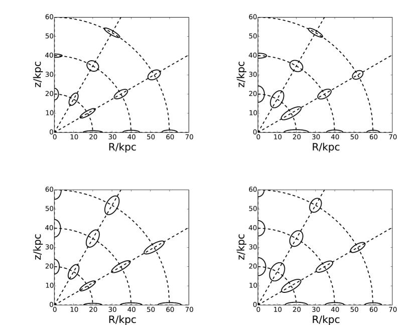
Figure 2: Velocity ellipsoids for flattened ($q=0.6$) Einasto profiles (upper panels) and power-law profiles (lower panels). The left column is for doubloon halos with $p=1$ (outer branch), the right column for $p=-1$ (inner branch). All the doubloon models have $V=200~{}\mbox{km s${}^{-1}$}$ and $a=50~{}\mbox{kpc}$. The Jeans solutions correspond to the case $K=1/40$. Notice that the flattened Einasto profiles do not have approximately invariant shapes, as the long axis of the velocity ellipsoid changes from radial to azimuthal at high latitudes.

3 Flattened Tracer Populations: Jeans Equations

For applications in which dark haloes are represented as doubloon models, we are primarily interested in the properties of flattened tracer populations of stars, whose kinematics are accessible to observation. The flattening is usually described by assuming a density law stratified on similar concentric spheroids with an axis ratio $q$. Tracers in haloes are often modelled with power-laws or broken power-laws (e.g., Watkins et al., 2009; Deason et al., 2011), which have asymptotic behaviour

$$\rho_{\mathrm{pl}}(r,\theta)\simeq Am^{-\delta},\quad m^{2}=r^{2}(\sin^{2}\theta+q^{-2}\cos^{2}\theta).$$ (34)

Another commonly used profile for luminous tracers, whether in stellar haloes or elliptical galaxies, is that due to J. Einasto (see e.g., Einasto & Haud, 1989; Deason et al., 2011), though it has also been used for the dark matter distribution (Graham et al., 2006). It has asymptotic behaviour

$$\rho_{\mathrm{Ein}}(r,\theta)\simeq A\exp(-sm^{1/n}),$$ (35)

where $s$ and $n$ are constants. This is the exponential profile if $n=1$ and the de Vaucouleurs-like profile if $n=4$. A convenient generalization that incorporates both families is the hyper-Einasto profile (cf. An & Zhao, 2013)

$$\rho_{\mathrm{HyEin}}(r,\theta)\simeq Am^{-\delta}\exp(-sm^{1/n}).$$ (36)

We shall solve the Jeans equations for both flattened power-law and hyper-Einasto tracers in dark matter haloes described by doubloon potentials. In an axisymmetric model, $\langle v_{r}v_{\phi}\rangle\equiv\langle v_{\theta}v_{\phi}\rangle\equiv 0$ by the symmetries of the individual orbits, which then leaves two non-trivial Jeans equations for the tracer density $\rho_{\rm t}(r,\theta)$ in terms of the spherical potential $\psi(r)$:

$$\begin{split}{\partial\rho_{\rm t}\langle v_{r}^{2}\rangle\over\partial r}+{1\over r}{\partial\rho_{\rm t}\langle v_{r}v_{\theta}\rangle\over\partial\theta}+{\rho_{\rm t}\over r}\Bigl{(}2\langle v_{r}^{2}\rangle-\langle v_{\theta}^{2}\rangle-\langle v_{\phi}^{2}\rangle+\langle v_{r}v_{\theta}\rangle\cot\theta\Bigr{)}\\ =\rho_{\rm t}{\partial\psi\over\partial r}=-\rho_{\rm t}{V^{2}r^{p-1}\over a^{p}+r^{p}},\end{split}$$ (37)

$${\partial\rho_{\rm t}\langle v_{r}v_{\theta}\rangle\over\partial r}+{1\over r}{\partial\rho_{\rm t}\langle v_{\theta}^{2}\rangle\over\partial\theta}+{\rho_{\rm t}\over r}\Bigl{[}3\langle v_{r}v_{\theta}\rangle+(\langle v_{\theta}^{2}\rangle-\langle v_{\phi}^{2}\rangle)\cot\theta\Bigr{]}=0.$$ (38)

These two relations between the four stresses $\rho\langle v_{r}^{2}\rangle$, $\rho\langle v_{r}v_{\theta}\rangle$, $\rho\langle v_{\theta}^{2}\rangle$, $\rho\langle v_{\phi}^{2}\rangle$ must be satisfied at any point in the model.

There is now increasing evidence from the stellar halo of our Galaxy that the velocity ellipsoid is spherically aligned. This was first noted by Smith et al. (2009a), who studied the kinematics of halo subdwarfs in the Sloan Digital Sky Survey Stripe 82, for which there is multi-epoch and multi-band photometry permitting the measurement of accurate proper motions. Subsequently, Bond et al. (2010) used $\sim 53000$ halo stars with $r$ band magnitude brighter than 20 and proper motion measurements derived from Sloan Digital Sky Survey and Palomar Observatory Sky Survey astrometry to extend this result over a quarter of the sky at high latitudes. Although the tilt of the velocity ellipsoid in elliptical galaxies is not known, galaxy modelling suggests that it is aligned on spheroidal coordinates (e.g., Binney, 2014), which become spherical at large radii. In other words, there is much motivation for investigating spherical alignment, $\langle v_{r}v_{\theta}\rangle=0$, as it holds good for the Milky Way’s stellar halo and for the outer parts of elliptical galaxies.

Additionally, there is good evidence from the kinematics of stars in the Milky Way’s stellar halo $\langle v_{\theta}^{2}\rangle\approx\langle v_{\phi}^{2}\rangle$. Smith et al. (2009b) found $\langle v_{\theta}^{2}\rangle^{1/2}=82\pm 2~{}\mbox{km s${}^{-1}$}$ and $\langle v_{\phi}^{2}\rangle^{1/2}=77\pm 2~{}\mbox{km s${}^{-1}$}$. Bond et al. (2010) claimed that the semi-axes are invariant over the volume probed by their much larger sample and found $\langle v_{\theta}^{2}\rangle^{1/2}=85\pm 5~{}\mbox{km s${}^{-1}$}$ and $\langle v_{\phi}^{2}\rangle^{1/2}=75\pm 5~{}\mbox{km s${}^{-1}$}$. It is interesting that the two angular semi-axes are almost the same. If the tracer population has a DF depending on $E$ and $L$ only, then $\langle v_{\theta}^{2}\rangle=\langle v_{\phi}^{2}\rangle$. We accordingly make this assumption, which has good theoretical and observational motivation, so that the Jeans equations become

$${\partial(r^{2}\rho_{\rm t}\langle v_{r}^{2}\rangle)\over\partial r}=r\rho_{\rm t}\Bigl{(}2\langle v_{\theta}^{2}\rangle-v_{\rm c}^{2}\Bigr{)},\quad{\partial(\rho_{\rm t}\langle v_{\theta}^{2}\rangle)\over\partial\theta}=0.$$ (39)

We see that this set of assumptions has closed the Jeans equations, which may now be integrated with suitable boundary conditions. Integrating the angular equation, we find $\rho_{\rm t}\langle v_{\theta}^{2}\rangle$ being an arbitrary function of $r$. As the boundary condition, we next assume that the velocity dispersion on the equatorial plane ($\theta=\pi/2$) is a constant fraction $K$ of the rotation curve, that is,

$$\langle v_{\theta}^{2}\rangle=\langle v_{\phi}^{2}\rangle=Kv_{\rm c}^{2}(r)\,{\rho_{\rm t}(r,\pi/2)\over\rho_{\rm t}(r,\theta)}$$ (40)

Assuming that $\rho\langle v_{r}^{2}\rangle\to 0$ as $r\to\infty$, we then have the full axisymmetric solution of the Jeans equations as

$$\langle v_{r}^{2}\rangle={1\over r^{2}\rho_{\rm t}(r,\theta)}\int_{r}^{\infty}\!{\rm d}x\,xv_{\rm c}^{2}(x)\,\Bigl{[}\rho_{\rm t}(x,\theta)-2K\rho_{\rm t}(x,\pi/2)\Bigr{]}$$ (41)

This gives a one-parameter family of solutions of the Jeans equations for axisymmetric densities with spherically aligned velocity dispersion tensors. Algorithms for cylindrically aligned Jeans solutions are known (Cappellari, 2008), although as Binney (2014) points out they are somewhat contrived. In cosmogonies in which galaxies are built from hierarchical merging, stellar material on nearly radial orbits fell in to deepening dark matter potential wells, and so spherically aligned Jeans solutions are much more natural. A general, though rather complicated, algorithm for spherically aligned Jeans solutions for flattened potential–density pairs is known (Bacon et al., 1983; Bacon, 1985). The assumption of a spherical potential, though, makes our algorithm much simpler for flattened tracer densities.

A necessary condition for everywhere positive stresses is that $0<K<1/2$. In practice, the range of physical $K$ values is much more constrained, though established easily enough by numerical integration. Fig. 2 shows velocity ellipsoids for power-law and Einasto profiles representing the stellar halo of the Milky Way. The Einasto profile has $n=1.7$ and an effective radius of $20~{}\mbox{kpc}$, the power law profile falls with $\delta=-4$ beyond a core radius of $0.6~{}\mbox{kpc}$. Both are inspired by fits to the stellar halo of the Milky Way discussed in Deason et al. (2011, 2014) and Evans & Williams (2014). The left column shows each tracer in a doubloon model with $p=-1$ (Jaffe, 1983), the right with $p=1$ (Evans & Williams, 2014). It is interesting to observe that the shape of the velocity ellipsoids is primarily controlled by the tracer density, with the power-law or Einasto profiles each generating similar Jeans solutions in different doubloon potentials. However, the shape of the velocity ellipsoids for power-laws tracers always has the radial velocity dispersion exceeding the angular velocity dispersions, so that the velocity ellipsoids are always prolate spheroids. This is not the case for the Einasto profiles, in which the azimuthal velocity dispersions exceeds the radial on approach to the poles ($\theta=0$), and so changes from prolate to oblate spheroidal in shape.

Although Deason et al. (2011, 2014) found either power-law or Einasto profiles equally good fits to the starcount data, it is obvious that the kinematics provides a powerful discriminant. The fact that the velocity ellipsoid shape is spherically aligned (Smith et al., 2009a) and (to first order) shape invariant over the Sloan Digital Sky Survey footprint (Bond et al., 2010) seems to rule out Einasto profiles. We plan to return to detailed Jeans solution fits to the kinematics of the stellar halo in a later publication.

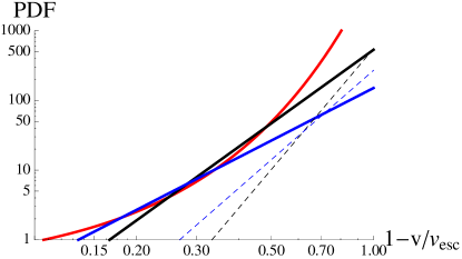
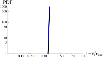
Figure 3: The probability density function of radial velocities near the escape speed for power-law (left) and Einasto (right) tracer densities. The logarithm of the probability density is plotted against $1-v/v_{\rm esc}$. The red line is for an isotropic power-law tracer with $\delta=5$ in a doubloon potential with $p=1$ (outer branch, the Evans & Williams (2014) model). The black and blue lines show tracers in a doubloon potential with $p=-1$ (inner branch, Jaffe model) with $\delta=5$ and $4$. Full and dashed lines show isotropic ($\beta=0$) and radially anisotropic ($\beta=0.5$) models. Although all four models are shown in the right panel, the super-exponential cut-off makes them virtually indistinguishable.

4 Tracer Populations: Distributions of High Velocity Stars

The high velocity stars of the Milky Way are distinct from the hyper-velocity stars. The central black hole may eject stars (Hills, 1988; Yu & Tremaine, 2003; Levin, 2006), which are often unbound and moving on highly radial orbits (Brown et al., 2014). These are the hyper-velocity stars, which are a separate population and do not form part of the steady-state stellar halo.

By contrast, the high velocity stars are the highest energy, but bound, members of the halo. The form of the distribution function at the highest energies is accessible to observational scrutiny and can in principle provide information on the behaviour of the potential at the edge. For example, in the Milky Way, the distribution of high-velocity stars from the halo is already available locally thanks to the RAVE survey (Smith et al., 2007; Piffl et al., 2014; Hawkins et al., 2015). One of the earliest investigations into the escape speed, Leonard & Tremaine (1990) introduced the simple and attractive ansatz that

$$\begin{cases}f(v)\propto(v_{\rm esc}-v)^{C}&(v<v_{\rm esc})\\ f(v)=0&(v>v_{\rm esc}),\end{cases}$$ (42)

where $f(v)$ is the distribution of space velocities near the escape speed $v_{\rm esc}$ and $C$ is a constant. This ansatz, which is exact for isotropic power-law DFs, has held up surprisingly well over the last quarter of a century (Piffl et al., 2014). However, the next few years will see the Gaia-ESO and LAMOST surveys, as well as the Gaia satellite, substantially improve our knowledge of the distribution of high velocity stars as a function of distance within 20 kpc of the Sun. Sample sizes of hundreds or even thousands of high velocity stars will become available, and deviations from equation (42) can be probed. Accordingly, we proceed to derive the form of the velocity distribution at the highest energies for power-law and hyper-Einasto tracers (defined in eq. 36).

4.1 Outer Branch

The highest velocity stars in the outer branch models correspond to the limit $E\to-\infty$, and we find $r(E)\simeq a{\rm e}^{|E|/V^{2}}\to\infty$ in the same limit. If the tracer density asymptotically becomes a power-law like $\rho\simeq Ar^{-\delta}$ as $r\to\infty$, then for $E\to-\infty$,

$$g\simeq 2^{\beta}Ar^{2\beta-\delta}\simeq 2^{\beta}Aa^{2\beta-\delta}\exp\biggl{(}\frac{(\delta-2\beta)E}{V^{2}}\biggr{)}.$$ (43)

We find that the asymptotic form of the constant anisotropy DF is

$$F\simeq\frac{2^{\beta}A}{(2\pi)^{3/2}a^{\delta-2\beta}}\biggl{(}\frac{\delta-2\beta}{V^{2}}\biggr{)}^{\frac{3}{2}-\beta}{L^{-2\beta}\over\Gamma(1-\beta)}\exp\biggl{(}-\frac{(\delta-2\beta)|E|}{V^{2}}\biggr{)}$$ (44)

for $E\to-\infty$. So, an isotropic power-law tracer ($\beta=0$) has an isothermal or a Maxwellian distribution of velocities. Even in the presence of anisotropy, the distribution of radial velocities remains a Maxwellian. The red line in the left panel of Fig. 3 shows the probability density function (PDF) of radial velocities near the escape speed derived from eq. (44) for the model with $\delta=5$ and $\beta=0$.

If the tracer population has an hyper-Einasto profile, then $g\simeq 2^{\beta}Ar^{2\beta-\delta}\exp(-sr^{1/n})$ as $r\to\infty$ and the DF asymptotically becomes

$$F\simeq\frac{2^{\beta}A}{(2\pi)^{3/2}a^{\delta-2\beta}}\biggl{(}\frac{sa^{1/n}}{nV^{2}}\biggr{)}^{\frac{3}{2}-\beta}{L^{-2\beta}\over\Gamma(1-\beta)}\\ \times\exp\Biggl{[}-sa^{\frac{1}{n}}{\rm e}^{\frac{|E|}{nV^{2}}}-\biggl{(}\delta-2\beta-\frac{3-2\beta}{2n}\biggr{)}\,\frac{|E|}{V^{2}}\Biggr{]}$$ (45)

as $E\to-\infty$. The distribution of space velocities is no longer Maxwellian, but rather is a Maxwellian modulated by a super-exponential cut-off.

4.2 Inner Branch

The forms of the high energy tail of the velocity distribution change if the dark matter density falls off like $r^{-3}$ or faster, as we now show. For $p<0$, Taylor expansion now shows that $r(E)\simeq a(V^{2}/|p|)^{1/|p|}E^{-1/|p|}\to\infty$ in the limit $E\to 0$. For power-law tracers, then as $r\to\infty$ and $E\to 0$,

$$g\simeq 2^{\beta}Ar^{2\beta-\delta}\simeq 2^{\beta}Aa^{2\beta-\delta}\biggl{(}\frac{|p|E}{V^{2}}\biggr{)}^{\chi}\quad(\text{where }\ \chi\equiv\frac{\delta-2\beta}{|p|})$$ (46)

which is also a power-law and so the asymptotic form of the DF is

$$F\simeq\frac{2^{\beta}A}{(2\pi)^{3/2}a^{\delta-2\beta}}\frac{\Gamma(\chi+1)}{\Gamma(\chi-1/2+\beta)}{L^{-2\beta}\over\Gamma(1-\beta)}E^{\beta-\frac{3}{2}}\biggl{(}\frac{|p|E}{V^{2}}\biggr{)}^{\chi}$$ (47)

for $E\to 0$. In other words, the space velocity distribution of a power-law tracer falls asymptotically like a power-law at the highest energies. The black and blue lines in the left panel of Fig. 3 show the PDF of radial velocities derived from equation (47) for the model with $\delta=5$ and $\delta=4$. Full lines are isotropic ($\beta=0$), dotted lines radially anisotropic ($\beta=1/2$).

For an Einasto tracer, a similar calculation yields

$$F\simeq\frac{2^{\beta}A}{(2\pi)^{3/2}a^{\delta-2\beta}}{L^{-2\beta}\over\Gamma(1-\beta)}\\ \times\biggl{(}\frac{sa^{1/n}}{n|p|E}\biggr{)}^{\frac{3}{2}-\beta}\biggl{(}\frac{|p|E}{V^{2}}\biggr{)}^{\frac{\delta-2\beta}{|p|}-\frac{3-2\beta}{2n|p|}}\exp\Biggl{[}-sa^{\frac{1}{n}}\biggl{(}\frac{V^{2}}{|p|E}\biggr{)}^{\frac{1}{n|p|}}\Biggr{]}$$ (48)

as $E\to 0$. So, the distribution of space velocities falls like a power-law with a super-exponential cut-off. The same four models ($\delta=5$ and $4$, and $\beta=0$ and $1/2$) are shown in the right panel of Fig. 3. The super-exponential cut-off causes all four model to lie on top of each other.

5 Conclusions

We have presented details of a new family of spherical models, which have properties suitable for mimicking galaxies with flattish rotation curves. The models may have a rotation curve which attains a finite value at the centre and falls on moving outwards. The archetype is the Jaffe (1983) model. Alternatively, the models can have a rising rotation curve in the inner parts, which flattens asymptotically. Here, the archetype is the spherical logarithmic model popularised by Binney & Tremaine (2008). The family also includes the singular isothermal sphere with an $\rho\sim r^{-2}$ density cusp at the center, as well as the halo model recently discovered by Evans & Williams (2014) which has an $r^{-1}$ cusp. In general, the family includes both cored and cusped members, and so can represent the range of cusps found in numerical simulations (see e.g., Moore et al., 1999).

The halo models presented here are spherical. Cosmological simulations suggest that dark halos are typically flattened and mildly oblate, with a ratio of long axis to short axis of $q=0.8$-$0.9$ (see e.g., Abadi et al., 2010; Deason et al., 2011; Zemp et al., 2012). For the Milky Way Galaxy, there are several lines of evidence suggesting that the dark halo may be nearly spherical. First, the fits to the tidal stream GD-1 using different methods (Koposov et al., 2010; Bowden et al., 2014) show that the total Galactic potential (disk and halo) at radii $\sim 15$ kpc is consistent with modest flattening. Secondly, the kinematics of halo subdwarfs in the Sloan Digital Sky Survey Stripe 82, for which there is multi-epoch and multi-band photometry permitting the measurement of accurate proper motions, is consistent with a nearly spherical potential (Smith et al., 2009a). Thirdly, the kinematics of the Sagittarius (Sgr) stream assuredly prohibit strongly flattened dark haloes with $q<0.6$ (Evans & Bowden, 2014). Whilst a definitive answer from Sgr stream kinematics must await a thorough exploration of stream generation in flattened haloes using modern algorithms (Gibbons et al, 2014), the debris of the Sgr stretches a full $360\degr$ over the sky and is almost confined to a plane.

The self-consistent distribution functions (DFs) in terms of the energy $E$ and angular momentum $L$ have been given for the models with constant anisotropy. There are however strong reasons for using actions, instead of integrals of the motion like energy, in DFs (Binney, 2013). Here, we note that Williams et al. (2014) have shown that the Hamiltonian as a function of actions in scale-free power-laws is an almost linear function of the actions, enabling schemes to be easily devised to convert the DFs into action space if desired. Evans & Williams (2014) provide a practical example of such an algorithm for one member of the doubloon family. Posti et al. (2015) and Williams & Evans (2015) give algorithms for action-based DFs for models with density falling like power-laws in certain regimes.

The self-consistent DFs describe the velocity distributions of dark matter needed to sustain the doubloon models. For applications to stars in stellar halos or in elliptical galaxies, we are interested in the properties of luminous tracers within the doubloon models. We have provided a number of results for both power-law and Einasto tracer populations. There is good evidence that the velocity dispersion tensor of the Milky Way’s stellar halo is aligned in spherical polar coordinates (Smith et al., 2009a; Bond et al., 2010). Additionally, the velocity ellipsoid of stellar populations in elliptical galaxies is probably aligned in spheroidal coordinates, which asymptotically become spherical. Therefore, spherically aligned Jeans solutions are of considerable astrophysical interest. We identify a simple algorithm for solving the spherically aligned Jeans equations for flattened tracers in spherical potentials, and provide solutions for power-law and hyper-Einasto tracers (defined in eq. 36).

The distribution of high velocity stars of the stellar halo of the Milky Way are becoming available (Smith et al., 2007; Piffl et al., 2014; Hawkins et al., 2015). So, we have provided the asymptotic forms of the DFs for tracer populations with power-law and Einasto density distributions. The form of the high velocity tail is particularly interesting as this may betray properties of the dark matter halo. Power-law tracers have velocity distributions with power-law or Maxwellian tails. Einasto tracers have super-exponential cut-offs in the velocity distributions. Although the observational data are often fitted to models like $f(v)\propto(v_{\rm esc}-v)^{k}$ this is only strictly correct for power-law tracers. If the stellar halo is described by an Einasto profile, then

$$\begin{cases}f(v)\propto(v_{\rm esc}-v)^{C}\exp\Bigl{[}-{\displaystyle A\over\displaystyle(v_{\rm esc}-v)^{B}}\Bigl{]}&v<v_{\rm esc}\\ f(v)=0&v>v_{\rm esc},\end{cases}$$ (49)

with $A,B$ and $C$ constants, is a better description of the high velocity tail near the escape speed. In principle, the different forms of the velocity distributions of tracers can provide us with evidence on the extent of the dark matter potential. This is a subject on which there is not merely little hard evidence, but very few avenues in which to gain evidence.

Appendix A Constant anisotropy models

A.1 Fractional calculus

Many of the formulae concerning the constant anisotropy DF can be swiftly derived using the notion of fractional differentiation. Let us consider the Riemann–Lioville integral (see Erdélyi et al., 1954):

$${{}^{+}_{a}I}_{x}^{\mu}f(x)\equiv\frac{1}{\Gamma(\mu)}\int_{a}^{x}\!{\rm d}y\,(x-y)^{\mu-1}f(y)\quad(\mu>0).$$ (50)

This generalizes Cauchy’s formula for repeated integration for an arbitrary positive order. This is also recognized as (generalized) Abel transform for $0<\mu<1$ with the classical case resulting from $\mu=1/2$. These obey the composition rule

$${{}^{+}_{a}I}_{x}^{\mu}\,{{}^{+}_{a}I}_{x}^{\xi}f(x)={{}^{+}_{a}I}_{x}^{\mu+\xi}f(x),$$ (51)

and the differentiation follows

$$\biggl{(}\frac{{\rm d}}{{\rm d}x}\biggr{)}^{n}{{}^{+}_{a}I}_{x}^{\mu}f(x)=\begin{cases}{{}^{+}_{a}I}_{x}^{\mu-n}f(x)&(n<\mu)\\ f(x)&(n=\mu)\end{cases}.$$ (52)

Thus the Riemann–Lioville integral may be inverted through

$$g(x)={{}^{+}_{a}I}_{x}^{\mu}f(x)\Rightarrow\ f(x)=\biggl{(}\frac{{\rm d}}{{\rm d}x}\biggr{)}^{\lfloor\mu\rfloor+1}{{}^{+}_{a}I}_{x}^{1-\epsilon}g(x)$$ (53)

where $\lfloor\mu\rfloor$ and $\epsilon\equiv\mu-\lfloor\mu\rfloor$ are the integer floor and the fraction part of $\mu$, respectively. Let us also define the fractional derivative:

$${{}_{a}\partial_{x}}^{\xi}f(x)\equiv\frac{\Gamma(\xi+1)}{2\pi{\rm i}}\int\limits_{a}^{(x+)}\frac{f(z)\,{\rm d}z}{(z-x)^{1+\xi}}$$ (54)

by means of the complex contour integral. Here, the contour starts and ends at the base point $a$, and encircles $x$ in the counter-clockwise direction. Thanks to Cauchy’s integral (and differentiation) formula, this coincides with the customary notion of differentiation for integer values of $\xi$, that is, ${{}_{a}\partial_{x}}^{0}f(x)=f(x)$ and ${{}_{a}\partial_{x}}^{n}f(x)=f^{(n)}(x)$ for $n\in\{1,2,\dotsc\}$. Explicit calculations can demonstrate that the fractional derivative is the inverse operator of the Riemann–Lioville integral, whereby

$${{}_{a}\partial_{x}}^{\xi}\,{{}^{+}_{a}I}_{x}^{\xi}f(x)=f(x),$$ (55)

and so follows that ${{}_{a}\partial_{x}}^{\xi}f(x)=({\rm d}/{\rm d}x)^{\lceil\xi\rceil}{{}^{+}_{a}I}_{x}^{\lceil\xi\rceil-\xi}f(x)$ where $\lceil\xi\rceil$ is the integer ceiling of $\xi$ and also assuming ${{}^{+}_{a}I}_{x}^{0}f(x)=f(x)$.

A.2 Constant anisotropy DF

Suppose that the DF is given by the ansatz of equation (12). The density profile results from the integral over the velocity,

$$\begin{split}\rho&=\iiint\!{\rm d}^{3}\!\mn@boldsymbol{v}\,F=\frac{2\pi}{r^{2}}\!\iint_{E\geq a,L^{2}\geq 0,v_{r}^{2}\geq 0}\!\frac{F(E,L^{2})\,{\rm d}E\,{\rm d}L^{2}}{\sqrt{v_{r}^{2}(E,L^{2};\psi,r)}}\\ &=(2r^{2})^{-\beta}\,{{}^{+}_{a}I}_{\psi}^{\frac{3}{2}-\beta}f_{E}(\psi),\end{split}$$ (56)

where and $a\equiv\psi(r_{0})$ if $r_{0}$ is the finite boundary radius or $a\equiv\lim_{r\to\infty}\psi(r)$. Hence if we define the augmented density

$$g(\psi)\equiv(2r^{2})^{\beta}\rho={{}^{+}_{a}I}_{\psi}^{\frac{3}{2}-\beta}f_{E}(\psi),$$ (57)

the energy part of the DF is inverted as

$$f_{E}(E)={{}_{a}\partial_{E}}^{\frac{3}{2}-\beta}g(E)=\biggl{(}\frac{{\rm d}}{{\rm d}E}\biggr{)}^{n+1}{{}^{+}_{a}I_{E}}^{1-\epsilon}g(E),$$ (58)

where $n=\lfloor(3/2-\beta)\rfloor$ and $\epsilon=3/2-\beta-n$, which may be compared with equation (3) of Evans & An (2006) (note the scale constants are chosen differently here). For the isotropic case ($\beta=0$), we have

$$(2\pi)^{3/2}F(E)={{}_{a}\partial_{\psi}}^{\frac{3}{2}}\rho(\psi)\bigr{|}_{\psi=E}=\frac{{\rm d}^{2}}{{\rm d}E^{2}}{{}^{+}_{a}I_{\psi}}^{\frac{1}{2}}\rho(\psi)\Bigr{|}_{\psi=E}$$ (59)

which reproduces Eddington’s (1916) formula, which can be thought of as the fractional derivative of order $3/2$.

For the DF of the form of equation (12), the energy part $f_{E}(E)$ is directly related to the local energy distribution

$$\frac{{\rm d}\rho}{{\rm d}E}=\frac{[\psi(r)-E]^{1/2-\beta}}{\Gamma(3/2-\beta)}\frac{f_{E}(E)}{(2r^{2})^{\beta}}$$ (60)

as well as the speed distribution

$$\frac{{\rm d}\rho}{{\rm d}v^{2}}=\frac{v^{1-2\beta}f_{E}[\psi(r)-v^{2}/2]}{2^{3/2}\Gamma(3/2-\beta)\,r^{2\beta}}.$$ (61)

Here also note that the local escape speed is given by $v_{\rm esc}=\sqrt{2\psi(r)}$ provided that $\lim_{r\to\infty}\psi(r)=0$.

A.3 Auxiliary results

For models on the outer branch, we make use of Hankel’s Loop integral for the reciprocal gamma function (see Erdélyi et al. 1953, eq.1.6(2); Olver et al. 2010, § 5.9(1)) indicating

$${{}_{-\infty}\partial_{E}}^{\lambda}{\rm e}^{sE}=\frac{\Gamma(\lambda+1)}{2\pi{\rm i}}\int\limits_{-\infty}^{(E+)}\frac{\exp(s\psi)\,{\rm d}\psi}{(\psi-E)^{1+\lambda}}=s^{\lambda}{\rm e}^{sE}.$$ (62)

For models on the inner branch however, we need to introduce the incomplete gamma function. The contour integral representation of the lower incomplete gamma function (cf. Erdélyi et al. 1953, eq.9.3(1); Olver et al. 2010, § 8.6(2)) implies

$$\begin{split}{{}_{0}\partial_{E}}^{\lambda}{\rm e}^{sE}&=\frac{\Gamma(\lambda+1)}{2\pi{\rm i}}\int\limits_{0}^{(E+)}\frac{\exp(s\psi)\,{\rm d}\psi}{(\psi-E)^{1+\lambda}}\\ &=s^{\lambda}{\rm e}^{sE}P(-\lambda,sE)=E^{-\lambda}{\rm e}^{sE}\gamma^{*}(-\lambda,sE)\end{split}$$ (63)

Here, $P(a,x)\equiv\gamma(a,x)/\Gamma(a)=x^{a}\gamma^{*}(a,x)$ is the regularized lower incomplete gamma function. If $\lambda$ is a positive integer, then $P(-\lambda,x)=1$ and so this is same as the ordinary $n$-th derivative. For a half-integer $\lambda$, this reduces to the error function (or Dawson’s integral, which is equivalent to the imaginary error integral) – note ${\rm erf}(x)=(1/\sqrt{\pi})\gamma(1/2,x^{2})=P(1/2,x^{2})$ and ${\rm erfi}(x)=-{\rm i}\,{\rm erf}({\rm i}x)$.

A.4 Constant anisotropy DFs of self-consistent Doubloons

For models on the outer branch, $p>0$ and $\phi<0$ and so $0<\varepsilon<1$ where $\varepsilon=\exp(p\psi/V^{2})$. Then $g(\psi)$ of equation (11) may be expanded to the power-series of $\varepsilon$ using binomial series;

$$\begin{split}g(\psi)&=\frac{C(\varepsilon+p\varepsilon^{2})}{\varepsilon^{-\lambda}}\sum_{j=0}^{\infty}\frac{(\lambda)_{j}}{j!}\varepsilon^{j}\\ &=C\left[\varepsilon^{\lambda+1}+\sum_{j=1}^{\infty}\biggl{(}\frac{(\lambda)_{j}}{j!}+\frac{p(\lambda)_{j-1}}{(j-1)!}\biggr{)}\,\varepsilon^{\lambda+1+j}\right],\end{split}$$ (64)

where $\lambda\equiv 2p^{-1}(1-\beta)-1$ and $C=2^{\beta-2}a^{2(\beta-1)}V^{2}/(\pi G)$. Equation (62) then indicates ${{}_{-\infty}\partial_{\psi}}^{\frac{3}{2}-\beta}\varepsilon^{\lambda+1+j}=V^{2\beta-3}[p(\lambda+1+j)]^{\frac{3}{2}-\beta}\varepsilon^{\lambda+1+j}$, and so equation (58) results in the DF in the form of equation (12) given by equation (13). For models on the inner branch, we have

$$g(\psi)=\tilde{g}({\rm e}^{-|p|\psi/V^{2}}),\quad\tilde{g}(\varepsilon)={C(1-|p|\varepsilon)(1-\varepsilon)^{\xi+1}\over\varepsilon^{\xi}},$$ (65)

where $\xi=2|p|^{-1}(1-\beta)\geq 0$. If $\beta=\frac{3}{2}-n$, equation (58) becomes

$$f_{E}(E)=\frac{{\rm d}^{n}g(E)}{{\rm d}E^{n}}=\biggl{(}-\frac{|p|\varepsilon}{V^{2}}\frac{{\rm d}}{{\rm d}\varepsilon}\biggr{)}^{n}\tilde{g}(\varepsilon)\Biggr{\rvert}_{\varepsilon=\exp(-|p|E/V^{2})},$$ (66)

which can be computed analytically. For others, we can still expand $\tilde{g}(\varepsilon)$ in a power series in $\varepsilon$ (note $0<\varepsilon<1$ since $p<0$ but $\psi>0$);

$$g(\psi)={C(1-|p|\varepsilon)\over\varepsilon^{\xi}}\sum_{j=0}^{\infty}{\xi+1\choose j}(-\varepsilon)^{j}.$$ (67)

Note, if $\xi$ is a non-negative integer, the sum terminates after the $j=\xi+1$ term and so reduces to a polynomial in $\varepsilon$. Given equation (63), applying equation (58) then results in $f_{E}(E)$ given as a sum over incomplete gamma functions, $P[\beta-\frac{3}{2},-(j-\xi)|p|\bar{\mathcal{E}}]$ where $\bar{\mathcal{E}}=E/V^{2}(\geq 0)$. If $\beta$ is an integer, these are reducible to the error function or Dawson’s integral, particular examples of which are provided in the main body.

References

- Abadi et al. (2010) Abadi M. G., Navarro J. F., Fardal M., Babul A., Steinmetz M., 2010, MNRAS, 407, 435
- Abramowitz & Stegun (1964) Abramowitz M., Stegun I., 1964, Handbook of Mathematical Functions, National Bureau of Standards, Washington DC (reprinted 1972, Dover, New York)
- An & Evans (2006a) An J. H., Evans N. W., 2006a, ApJ, 642, 752
- An & Evans (2006b) An J. H., Evans N. W., 2006b, A&A, 444, 45
- An & Zhao (2013) An J., Zhao H., 2013, MNRAS, 428, 2805
- Bacon et al. (1983) Bacon R., Simien F., Monnet G., 1983, A&A, 128, 405
- Bacon (1985) Bacon R., 1985, A&A, 143, 84
- Binney (1981) Binney J. J., 1981, MNRAS, 196, 455
- Binney (2013) Binney J. J., 2013, New Astron. Rev., 57, 29
- Binney (2014) Binney J., 2014, MNRAS, 440, 787
- Binney & Tremaine (2008) Binney J., Tremaine S., 2008, Galactic Dynamics, 2nd edn. Princeton University Press, Princeton
- Bond et al. (2010) Bond N. A., Ivezić Ž., Sesar B., et al., 2010, ApJ, 716, 1
- Bowden et al. (2014) Bowden A., Belokurov V., Evans N. W., 2014, MNRAS, arXiv1502.00484
- Brown et al. (2014) Brown W. R., Geller M. J., Kenyon S. J., 2014, ApJ, 787, 89
- Cappellari (2008) Cappellari M., 2008, MNRAS, 390, 71
- Chandrasekhar (1939) Chandrasekhar S., 1939, An Introduction to the Study of Stellar Structure, the University of Chicago Press, Chicago (reprinted 1958, reissued 2010, Dover, New York)
- Deason et al. (2011) Deason A. J., Belokurov V., Evans N. W., 2011, MNRAS, 416, 2903
- Deason et al. (2011) Deason A. J., et al., 2011, MNRAS, 415, 2607
- Deason et al. (2014) Deason A. J., Belokurov V., Koposov S. E., Rockosi C. M., 2014, ApJ, 787, 30
- Dehnen (1993) Dehnen W., 1993, MNRAS, 265, 250
- Eddington (1916) Eddington A. S., 1916, MNRAS, 76, 572
- Einasto & Haud (1989) Einasto J., Haud U., 1989, A&A, 223, 89
- Erdélyi et al. (1953) Erdélyi A., Magnus W., Oberhettinger F., Tricomi F., 1953, Higher Transcendental Functions, McGraw-Hill, New York
- Erdélyi et al. (1954) Erdélyi A., Magnus W., Oberhettinger F., Tricomi F., 1954, Tables of Integral Transforms, McGraw-Hill, New York
- Evans (1993) Evans N. W., 1993, MNRAS, 260, 191
- Evans & An (2005) Evans N. W., An J., 2005, MNRAS, 360, 492
- Evans & An (2006) Evans N. W., An J. H., 2006, Phys. Rev. D, 73, 023524
- Evans & Bowden (2014) Evans N. W., Bowden A., 2014, MNRAS, 443, 2
- Evans & Williams (2014) Evans N. W., Williams A. A., 2014, MNRAS, 443, 791
- Fridman & Polyachenko (1984) Fridman A. M., Polyachenko V., 1984, Physics of Gravitating Systems, Springer Verlag, Berlin
- Gerhard et al. (1998) Gerhard O. E., Jeske G., Saglia R. P., Bender R. 1998, MNRAS, 295, 197
- Gibbons et al (2014) Gibbons S., Belokurov V., Evans N. W., 2014, MNRAS, 445, 3788
- Graham et al. (2006) Graham A. W., Merritt D., Moore B., Diemand J., Terzic B., 2006, AJ, 132, 2701
- Hansen & Moore (2006) Hansen S., Moore B., 2006, New Astron., 11, 333
- Hawkins et al. (2015) Hawkins K., et al., 2015, MNRAS, 447, 2046
- Hernquist (1990) Hernquist L., 1990, ApJ, 356, 359
- Hernquist & Ostriker (1992) Hernquist L., Ostriker J. P., 1992, ApJ, 386, 375
- Hills (1988) Hills J. G., 1988, Nature, 331, 687
- Iguchi et al. (2006) Iguchi O., Sota Y., Nakamichi A., Morikawa M. 2006, Phys Rev E, 73, 046112
- Jaffe (1983) Jaffe W., 1983, MNRAS, 202, 995
- Jeans (1919) Jeans J. H., 1919, Problems of Cosmogony and Stellar Dynamics, Cambridge University Press, Cambridge
- Kochanek (1996) Kochanek C., 1996, ApJ, 457, 228
- Koposov et al. (2010) Koposov S., Rix H. W., Hogg D., 2010, ApJ, 712, 260
- Leonard & Tremaine (1990) Leonard P. J. T., Tremaine S., 1990, ApJ, 353, 486
- Levin (2006) Levin Y., 2006, ApJ, 653, 1203
- Merritt (1985a) Merritt D., 1985a, MNRAS, 214, 25P
- Merritt (1985b) Merritt D., 1985b, AJ, 90, 1027
- Mo, van den Bosch & White (2010) Mo H., van den Bosch F., White S. D. M., 2010, Galaxy Formation and Evolution, Cambridge University Press, Cambridge
- Moore et al. (1999) Moore B., Quinn T., Governato F., Stadel J., Lake G., 1999, MNRAS, 310, 1147
- Olver et al. (2010) Olver F. W. J., Lozier D. W., Boisvert R. F., Clark C. W., 2010, NIST Handbook of Mathematical Functions. Cambridge University Press, Cambridge (http://dlmf.nist.gov)
- Osipkov (1979) Osipkov, L. P., 1979, Pisma Astron. Zh., 5, 77
- Palmer & Papaloizou (1987) Palmer P. L, Papaloizou J. C. B., 1987, MNRAS, 224, 1043
- Piffl et al. (2014) Piffl T., et al., 2014, A&A, 562, A91
- Plummer (1911) Plummer H. C., 1911, MNRAS, 71, 460
- Posti et al. (2015) Posti L., Binney J., Nipoti C., Ciotti L., 2015, MNRAS, 447, 3060
- Sota et al. (2008) Sota Y., Iguchi O., Tashiro T., Morikawa M.. 2008, Phys Rev E, 77, 05117
- Smith et al. (2007) Smith M. C., et al., 2007, MNRAS, 379, 755
- Smith et al. (2009a) Smith M. C., Evans N. W., An J. H., 2009a, ApJ, 698, 1110
- Smith et al. (2009b) Smith M. C., et al., 2009b, MNRAS, 399, 1223
- Tremaine et al. (1994) Tremaine S., Richstone D. O., Byun Y.-I., et al., 1994, AJ, 107, 634
- Watkins et al. (2009) Watkins L. L., et al., 2009, MNRAS, 398, 1757
- Wilkinson & Evans (1999) Wilkinson M., Evans N. W., 1999, MNRAS, 310, 645
- Williams & Evans (2015) Williams A. A., Evans N. W., 2015, MNRAS, 448, 1360
- Williams et al. (2014) Williams A. A., Evans N. W., Bowden A., 2014, MNRAS 442, 1405
- Yu & Tremaine (2003) Yu Q., Tremaine S., 2003, ApJ, 599, 1129
- Zemp et al. (2012) Zemp M., Gnedin O. E., Gnedin N. Y., Kravtsov A. V., 2012, ApJ, 748, 54