Bio-Inspired Framework for Allocation of Protection Resources in Cyber-Physical Networks

Chapter 1 Introduction

Understanding spreading processes in complex networks and designing control strategies to contain them are relevant problems in many different settings, such as epidemiology and public health [4], computer viruses [23], information propagation in social networks [44], or security of cyberphysical networks [73]. In this chapter, we describe a bio-inspired framework for optimal allocation of resources to prevent spreading processes in complex cyber-physical networks. Our motivation is inspired by recent advancement on the problem of containing epidemics in human contact networks. The most popular dynamic epidemic model is the Susceptible-Infected-Susceptible (SIS) model [1, 35]. In this model, a given population is divided into two compartments. The first compartment, called ‘Susceptible’ ($S$), contains individuals who are healthy, but susceptible to becoming infected. The second compartment is called ‘Infected’ ($I$) and contains individuals who are infected and able to recover from the disease. Individuals can transition from $S$ to $I$ as they become infected, and from $I$ to $S$ as they recover. In addition to the SIS model, there are many other models able to model more realistic spreading processes. This is often done by adding extra compartments representing a variety of disease stages. There are many works that analyze different variations of the SIS model, such as extensions to higher number of disease states [76, 21, 39, 58, 59, 10, 32], or explicit modeling of birth and mortality rates [30, 45]. Stability results are obtained in [40, 41, 45] using Lyapunov analysis, or in [31] using Volterra integral models.

In the literature, we find several approaches to model spreading mechanisms in arbitrary contact networks. The analysis of this question in arbitrary (undirected) contact networks was first studied by Wang et al. [84] for a Susceptible-Infected-Susceptible (SIS) discrete-time model. In [22], Ganesh et al. studied the epidemic threshold in a continuous-time SIS spreading processes. In both continuous- and discrete-time models, there is a close connection between the speed of the spreading and the spectral radius of the network (i.e., the largest eigenvalue of its adjacency matrix) [79]. Designing strategies to contain spreading processes in networks is a central problem in public health and network security. In this context, the following question is of particular interest: given a contact network (possibly weighted and/or directed) and resources that provide partial protection (e.g., vaccines and/or antidotes), how should one distribute these resources throughout the network in a cost-optimal manner to contain the spread? This question has been addressed in several papers. Cohen et al. [18] proposed a heuristic vaccination strategy called acquaintance immunization policy and proved it to be much more efficient than random vaccine allocation. In [7], Borgs et al. studied theoretical limits in the control of spreads in undirected network with a non-homogeneous distribution of antidotes. Chung et al. [17] studied a heuristic immunization strategy based on the PageRank vector of the contact graph. In the control systems literature, Wan et al. proposed in [81, 82] a method to design control strategies by allocating heterogeneous resources in undirected networks. In [67], the authors present an spectral analysis of proximity random graphs with applications to virus spread. In [26], the authors study the problem of minimizing the level of infection in an undirected network using corrective resources within a given budget. In [61] a linear-fractional optimization program was proposed to compute the optimal investment on disease awareness over the nodes of a social network to contain a spreading process. In particular, we will cover in detail the work in [65, 66, 64, 69], where the authors developed a convex formulation to find the optimal allocation of protective resources in a network. An analysis of greedy control strategies and worst-case conditions was presented in [87]. Recent extensions include the analysis of more general epidemic models [52], competing diseases [16, 85, 50], time-switching networks [53, 57, 55], and non-Poissonian spreading and recovery rates [54, 56] have been recently developed. A novel data-driven optimization framework has also been recently proposed by Han et al. in [28]. A distributed framework for optimal allocation of resources has also been proposed in [70]. A novel analysis of epidemic models in arbitrary graphs using tools from positive systems can be found in [38].

In this Chapter, we describe an optimization-based framework to find the optimal allocation of protection resources in weighted and directed networks of nonidentical agents in polynomial time. In our study, we consider two types of containment resources:

• Preventive resources able to protect (or ‘immunize’) nodes against the spreading (such as vaccines in a viral infection process). This type of resources are allocated in nodes and/or edges of the network before the spread has reached them, so that this element is protected from the spread. The effect of this resource is to reduce the rate in which the spread can reach this element.

• Corrective resources able to neutralize the spreading after it has reached a node (such as antidotes in a viral infection). Notice that, in contrast with preventive resources, corrective resources are used after the spread has reached a node in the network. The effect of this type of resource is to increase the rate of recovery of an elements after the spread has reached it.

In the framework herein presented, we assume there are cost associated with these resources and study the problem of finding the cost-optimal distribution of resources throughout the network to contain the spreading. The aforementioned protection resources have an associated cost that depends on the level of protection achieved by the resource. For example, the larger the investment on vaccines and antidotes, the higher the level of protection achieved by the population in which the resources have been distributed. One of the main questions in epidemiology and public health is to find the optimal allocation of preventive and corrective resources to contain an epidemic outbreak in a cost-optimal manner. An identical question can be asked in the context of designing protection strategies for other cyber-physical networks, motivating the main problem covered in this chapter:

Problem.

Find the cost-optimal allocation of preventive and corrective resources to protect a cyber-physical network against spreading processes.

In the field of systems reliability, there is a well-developed theory of preventive and corrective maintenance for single components or machines, but there is a lack of a theoretical framework to analyze large-scale interdependent systems [71]. The state-of-the-art in the reliability analysis of networked systems is mostly based on Markov models [33, 72, 71, 20]. These models usually suffer from scalability issues, since the state space grows exponentially fast with the number of components under consideration. Similar Markov models have also been proposed in the analysis of disease spreading in networked populations. A rich and growing literature is arising in this context, proposing a variety of approaches to find efficient allocation of protection resources to contain an epidemic outbreak. In a series of papers, Preciado et al. developed a mathematical framework, based on dynamic systems theory and convex optimization, to find the optimal distribution of protection resources in a complex network [63, 65, 62, 68]. In particular, they showed that it is possible to find the cost-optimal distribution of vaccines and antidotes in a (possibly weighted and directed) social network of nonidentical nodes in polynomial time using geometric programming [66]. This framework has also be extended to find the allocation of traffic-control resources to find the cost-optimal traffic profile in a transportation network to contain the spread of a disease among cities [64].

1.1 Mathematical Framework

We introduce notation and preliminary results needed in our derivations. In the rest of the paper, we denote by $\mathbb{R}_{+}^{n}$ (respectively, $\mathbb{R}_{++}^{n}$) the set of $n$-dimensional vectors with nonnegative (respectively, positive) entries. We denote vectors using boldface letters and matrices using capital letters. $I$ denotes the identity matrix and $\mathbf{1}$ the vector of all ones. $\Re\left(z\right)$ denotes the real part of $z\in\mathbb{C}$.

1.1.1 Graph Theory

A weighted, directed graph (also called digraph) is defined as the triad $\mathcal{G}\triangleq\left(\mathcal{V},\mathcal{E},\mathcal{W}\right)$, where (i) $\mathcal{V}\triangleq\left\{v_{1},\dots,v_{n}\right\}$ is a set of $n$ nodes, (ii) $\mathcal{E}\subseteq\mathcal{V}\times\mathcal{V}$ is a set of ordered pairs of nodes called directed edges, and (iii) the function $\mathcal{W}:\mathcal{E}\rightarrow\mathbb{R}_{++}$ associates positive real weights to the edges in $\mathcal{E}$. By convention, we say that $\left(v_{j},v_{i}\right)$ is an edge from $v_{j}$ pointing towards $v_{i}$. We define the in-neighborhood of node $v_{i}$ as $\mathcal{N}_{i}^{in}\triangleq\left\{j:\left(v_{j},v_{i}\right)\in\mathcal{E}\right\}$, i.e., the set of nodes with edges pointing towards $v_{i}$. We define the weighted in-degree (resp., out-degree) of node $v_{i}$ as $\deg_{in}\left(v_{i}\right)\triangleq\sum_{j\in\mathcal{N}_{i}^{in}}\mathcal{W}\left(\left(v_{j},v_{i}\right)\right)$ (resp., $\deg_{out}\left(v_{i}\right)\triangleq\sum_{j\in\mathcal{N}_{i}^{out}}\mathcal{W}\left(\left(v_{j},v_{i}\right)\right)$); in other words, the weighted degrees are the sum of the edge weights attached to a node.

The adjacency matrix of a weighted, directed graph $\mathcal{G}$, denoted by $A_{\mathcal{G}}=[a_{ij}]$, is a $n\times n$ matrix defined entry-wise as $a_{ij}=\mathcal{W}((v_{j},v_{i}))$ if edge $(v_{j},v_{i})\in\mathcal{E}$, and $a_{ij}=0$ otherwise [5]. Given a $n\times n$ matrix $M$, we denote by $\mathbf{v}_{1}\left(M\right),\ldots,\mathbf{v}_{n}\left(M\right)$ and $\lambda_{1}\left(M\right),\ldots,\lambda_{n}\left(M\right)$ the set of eigenvectors and corresponding eigenvalues of $M$, respectively, where we order them in decreasing order of their real parts, i.e., $\Re\left(\lambda_{1}\right)\geq\Re\left(\lambda_{2}\right)\geq\ldots\geq\Re\left(\lambda_{n}\right)$. We call $\lambda_{1}\left(M\right)$ and $\mathbf{v}_{1}\left(M\right)$ the dominant eigenvalue and eigenvector of $M$. The spectral radius of $M$, denoted by $\rho\left(M\right)$, is the maximum modulus of an eigenvalue of $M$.

In this paper, we only consider graphs with positively weighted edges; hence, the adjacency matrix of a graph is always nonnegative. Conversely, given a $n\times n$ nonnegative matrix $A$, we can associate a directed graph $\mathcal{G}_{A}$ such that $A$ is the adjacency matrix of $\mathcal{G}_{A}$. Finally, a nonnegative matrix $A$ is irreducible if and only if its associated graph $\mathcal{G}_{A}$ is strongly connected.

In our derivations, we use Perron-Frobenius lemma, from the theory of nonnegative matrices [49]:

Lemma 1.1.1.

(Perron-Frobenius) Let $M$ be a nonnegative, irreducible matrix. Then, the following statements about its spectral radius, $\rho\left(M\right)$, hold:

(a) $\rho\left(M\right)>0$ is a simple eigenvalue of $M$,

(b) $M\mathbf{u}=\rho\left(M\right)\mathbf{u}$, for some $\mathbf{u}\in\mathbb{R}_{++}^{n}$, and

(c) $\rho\left(M\right)=\inf\left\{\lambda\in\mathbb{R}:M\mathbf{u}\leq\lambda\mathbf{u}\mbox{ for }\mathbf{u}\in\mathbb{R}_{++}^{n}\right\}$.

Remark 1.1.1.

Since a matrix $M$ is irreducible if and only if its associated digraph $\mathcal{G}_{M}$ is strongly connected, the above lemma also holds for the spectral radius of the adjacency matrix of any (positively) weighted, strongly connected digraph.

Corollary 1.1.2.

Let $M$ be a nonnegative, irreducible matrix. Then, its eigenvalue with the largest real part, $\lambda_{1}\left(M\right)$, is real, simple, and equal to the spectral radius $\rho\left(M\right)>0$.

1.1.2 Stochastic Spreading Model in Arbitrary Networks

We formulate the simplest version of the problem under consideration using a generalization of the SIS model, popularly used to model spreading dynamics in networks, such as the propagation of diseases in a networked population [42, 14, 79] or malware in a compute network [36, 37, 83, 24]. This generalization of the SIS model, called Heterogeneous Networked SIS model (HeNeSIS), is a continuous-time networked Markov process in which each node in the network can be in one out of two possible states, namely, susceptible or infected. In the context of systems reliability, each node in the networked Markov process represents a component in a networked infrastructure, and the susceptible and infected states correspond to operational and faulty states of these components, respectively. Over time, each node $v_{i}\in\mathcal{V}$ in the networked Markov process can change its state according to a stochastic process parameterized by (i) the edge propagation rate $\beta_{ij}$, and (ii) its node recovery rate $\delta_{i}$. In what follows, we shall describe the dynamics of the HeNeSIS model.

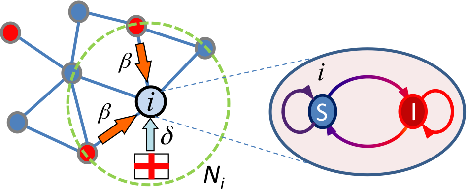
Figure 1.1: Networked Markov process with 2 states per node, corresponding to the HeNeSIS spreading model. Infected (resp., susceptible) nodes are plotted in red (resp., blue).

The dynamics of the HeNeSIS model can be described as follows. The state of node $v_{i}$ at time $t\geq 0$ is a binary random variable $X_{i}\left(t\right)\in\{0,1\}$. The state $X_{i}\left(t\right)=0$ (resp., $X_{i}\left(t\right)=1$) indicates that node $v_{i}$ is in the susceptible (resp., infected) state. We define the vector of states as $X\left(t\right)=\left(X_{1}\left(t\right),\ldots,X_{n}\left(t\right)\right)^{T}$. The state of a node can experience two possible stochastic transitions:

1. Assume node $v_{i}$ is in the susceptible state at time $t$. This node can switch to the infected state during the time interval $\left[t,t+\Delta t\right)$ with a probability that depends on: (i) the propagation rates $\left\{\beta_{ij},\mbox{ for }j\in\mathcal{N}_{i}^{in}\right\}$, and (iii) the states of its in-neighbors $\left\{X_{j}\left(t\right),\mbox{ for }j\in\mathcal{N}_{i}^{in}\right\}$. Formally, the probability of this transition is given by

   $$\Pr\left(X_{i}(t+\Delta t)=1|X_{i}(t)=0,X(t)\right)=\sum_{j\in\mathcal{N}_{i}^{in}}\beta_{ij}X_{j}\left(t\right)\Delta t+o(\Delta t),$$ (1.1)

   where $\Delta t>0$ is considered an asymptotically small time interval.

2. Assuming node $v_{i}$ is infected, the probability of $v_{i}$ recovering back to the susceptible state in the time interval $\left[t,t+\Delta t\right)$ is given by

   $$\Pr(X_{i}(t+\Delta t)=0|X_{i}(t)=1,X(t))=\delta_{i}\Delta t+o(\Delta t),$$ (1.2)

   where $\delta_{i}>0$ is the curing rate of node $v_{i}$.

In the context of failure propagation in networked infrastructure, $\beta_{ij}$ represents the Poisson rate at which a failure in the element located at node $v_{j}$ propagates to the element in node $v_{i}$. Similarly, $\delta_{i}$ represents the Poisson rate at which a fault at component $v_{i}$ is cleared. This HeNeSIS model is therefore a continuous-time Markov process with $2^{n}$ states in the limit $\Delta t\to 0^{+}$. Unfortunately, the exponentially increasing state space makes this model hard to analyze for large-scale networks. Using the Kolmogorov forward equations and a mean-field approach [79], one can approximate the dynamics of the spreading process using a system of $n$ ordinary differential equations, as follows. Let us define $p_{i}\left(t\right)\triangleq\Pr\left(X_{i}\left(t\right)=1\right)=E\left(X_{i}\left(t\right)\right)$, i.e., the probability of node $v_{i}$ being infected (or faulty) at time $t$. Hence, the Markov differential equation [77] for the state $X_{i}\left(t\right)=1$ is the following,

$$\frac{dp_{i}\left(t\right)}{dt}=\left(1-p_{i}\left(t\right)\right)\sum_{j=1}^{n}\beta_{ij}p_{j}\left(t\right)-\delta_{i}p_{i}\left(t\right).$$ (1.3)

Considering $i=1,\ldots,n$, we obtain a system of nonlinear differential equation with a complex dynamics. In the following, we derive a sufficient condition for the spreading process to die out exponentially fast. Let us define the vector $\mathbf{p}\left(t\right)\triangleq\left(p_{1}\left(t\right),\ldots,p_{n}\left(t\right)\right)^{T}$, and the matrices $B_{\mathcal{G}}\triangleq\left[\beta_{ij}\right]$, $D\triangleq\mbox{diag}\left(\delta_{i}\right)$. Notice that $B_{\mathcal{G}}$ is the weighted adjacency matrix of a weighted, directed graph with edge-weight function $\mathcal{W}\left(v_{j}\to v_{i}\right)=\beta_{ij}$; in other words, the weights of the directed link from $v_{j}$ to $v_{i}$ is $\beta_{ij}$. The ODE under consideration presents an equilibrium point at $\mathbf{p}^{*}=0$, called the disease-free (or fault-free) equilibrium. A stability analysis of this ODE around the equilibrium provides the following stability result [65]:

Proposition 1.

Consider the nonlinear HeNeSIS model in (1.3) and assume $\beta_{ij},\delta_{i}>0$. Then, if the eigenvalue with largest real part of $B_{\mathcal{G}}-D$ satisfies

$$\Re\left[\lambda_{1}\left(B_{\mathcal{G}}-D\right)\right]\leq-\varepsilon,$$ (1.4)

for some $\varepsilon>0$, the disease-free equilibrium ($\mathbf{p}^{*}=\boldsymbol{0}$) is globally exponentially stable, i.e., $\left\|\mathbf{p}\left(t\right)\right\|\leq\left\|\mathbf{p}\left(0\right)\right\|K\exp\left(-\varepsilon t\right)$, for some $K>0$.

1.2 A Quasiconvex Framework for Optimal Resource Allocation

Assume that the fault propagation and recovery rates, $\beta_{ij}$ and $\delta_{i}$, are adjustable by allocating protection resources on the edges and nodes of the networked Markov process. We consider two types of protection resources: (i) preventive resources (e.g., vaccinations in the case of disease spreading), and (ii) corrective resources (e.g., antidotes). We assume that the propagation rate $\beta_{ij}$ can be reduced using preventive resources. Also, allocating corrective resources at node $v_{i}$ increases the recovery rate $\delta_{i}$. We assume that we are able to, simultaneously, modify the fault propagation and recovery rates of $v_{i}$ within feasible intervals $0<\underline{\beta}_{ij}\leq\beta_{ij}\leq\bar{\beta}_{ij}$ and $0<\underline{\delta}_{i}\leq\delta_{i}\leq\bar{\delta}_{i}<\Delta$, where $\Delta$ is an uniform upper bound in the achievable recovery rate, which is assumed to be known a priori. The particular values of $\beta_{ij}$ and $\delta_{i}$ depend on the amount of preventive and corrective resources allocated at node $v_{i}$. We consider that protection resources have an associated cost. We define two cost functions, the prevention (or vaccination) cost function $f_{ij}\left(\beta_{ij}\right)$ and the correction (or antidote) cost function $g_{i}\left(\delta_{i}\right)$, that account for the cost of tuning the fault propagation and recovery rates to $\beta_{ij}\in\left[\underline{\beta}_{ij},\bar{\beta}_{ij}\right]$ and $\delta_{i}\in\left[\underline{\delta}_{i},\bar{\delta}_{i}\right]$, respectively.

In this context of protection design, one can study a type of resource allocation problems, called the budget-constrained allocation problem. In the budget-constrained problem we are assigned a total budget $C$ to invest on protection resources and we need to find the best allocation of preventive and/or corrective resources to maximize a measure of the network resilience. In [65] and [66], the authors proposed a measure of the network resilience based on the norm of the vector of probabilities of fault probabilities, $\left\|\mathbf{p}\left(t\right)\right\|$. In particular, the exponential rate of decay of such a vector is a measure of the ability of the networked infrastructure to recover from random failures. In other words, assuming that we are able to control the system to satisfy the condition $\left\|\mathbf{p}\left(t\right)\right\|\leq\left\|\mathbf{p}\left(0\right)\right\|K\exp\left(-\varepsilon t\right)$, the exponential decay rate $\varepsilon$ measures the ability of the networked infrastructure to ‘self-heal’ from random contingencies.

Based on Proposition 1, the decay rate of an epidemic outbreak is determined by $\varepsilon$ in (1.4). Thus, given a budget $C$, the budget-constrained allocation problem is formulated as follows:

Problem 1.

(Budget-constrained allocation) Given the following elements: (i) A directed network $\mathcal{G}=\left(\mathcal{V},\mathcal{E}\right)$ representing failure dependencies between components in a networked infrastructure, (ii) a set of cost functions $f_{ij}\left(\beta_{ij}\right)$,$g_{i}\left(\delta_{i}\right)$, (iii) bounds on the fault propagation and recovery rates $0<\underline{\beta}_{ij}\leq\beta_{ij}\leq\overline{\beta}_{ij}$ and $0<\underline{\delta}_{i}\leq\delta_{i}\leq\overline{\delta}_{i}$, and (iv) a total budget $C$, find the cost-optimal distribution of (preventive and corrective) protection resources to maximize the exponential decay rate $\varepsilon$.

Based on Proposition 1, we can state this problem as the following optimization program:

$$\underset{{\scriptscriptstyle\varepsilon,\left\{\beta_{ij}\right\}_{\left(j,i\right)\in\mathcal{E}},\left\{\delta_{i}\right\}_{i=1}^{n}}}{\mbox{maximize }} \varepsilon$$ (1.5)

subject to $$\Re\left[\lambda_{1}\left(B_{\mathcal{G}}-D\right)\right]\leq-\varepsilon,$$ (1.6)

$$\sum_{\left(j,i\right)\in\mathcal{E}}f_{ij}\left(\beta_{ij}\right)+\sum_{i\in\mathcal{V}}g_{i}\left(\delta_{i}\right)\leq C,$$ (1.7)

$$\underline{\beta}_{ij}\leq\beta_{ij}\leq\overline{\beta}_{ij},\mbox{ }\left(j,i\right)\in\mathcal{E};\mbox{ }\underline{\delta}_{i}\leq\delta_{i}\leq\overline{\delta}_{i},\mbox{ }i\in\mathcal{V},$$ (1.8)

where (1.7) is the budget constraint.

In the following section, we propose an approach to find the optimal budget-constraint allocation in polynomial time for weighted and directed contact networks, under certain convexity assumptions on the cost functions $f_{ij}$ and $g_{i}$.

1.2.1 A Geometric Programming Approach

We propose a convex formulation to solve the budget-constrained in weighted, directed networks using geometric programming (GP) [9]. Geometric programs are a type of quasiconvex optimization problems that can be easily transformed into convex programs and solved in polynomial time. We start our exposition by briefly reviewing some concepts used in our formulation. Let $x_{1},\ldots,x_{n}>0$ denote $n$ decision variables and define $\mathbf{x}\triangleq\left(x_{1},\ldots,x_{n}\right)\in\mathbb{R}_{++}^{n}$. In the context of GP, a monomial $h(\mathbf{x})$ is defined as a real-valued function of the form $h(\mathbf{x})\triangleq dx_{1}^{a_{1}}x_{2}^{a_{2}}\ldots x_{n}^{a_{n}}$ with $d>0$ and $a_{i}\in\mathbb{R}$. A posynomial function $q(\mathbf{x})$ is defined as a sum of monomials, i.e., $q(\mathbf{x})\triangleq\sum_{k=1}^{K}c_{k}x_{1}^{a_{1k}}x_{2}^{a_{2k}}\ldots x_{n}^{a_{nk}}$, where $c_{k}>0$. Posynomials are closed under addition, multiplication, and nonnegative scaling. A posynomial can be divided by a monomial, with the result a posynomial.

A geometric program (GP) is an optimization problem of the form (see [8] for a comprehensive treatment):

minimize $$f(\mathbf{x})$$ (1.9)

subject to $$q_{i}(\mathbf{x})\leq 1,\>i=1,...,m,$$

$$h_{i}(\mathbf{x})=1,\>i=1,...,p,$$

where $q_{i}$ are posynomial functions, $h_{i}$ are monomials, and $f$ is a convex function in log-scale. A GP is a quasiconvex optimization problem [9] that can be transformed to a convex problem. This conversion is based on the logarithmic change of variables $y_{i}=\log x_{i}$, and a logarithmic transformation of the objective and constraint functions (see [8] for details on this transformation). After this transformation, the GP in (1.9) takes the form

minimize $$F\left(\mathbf{y}\right)$$ (1.10)

subject to $$Q_{i}\left(\mathbf{y}\right)\leq 0,\>i=1,...,m,$$

$$\mathbf{b}_{i}^{T}\mathbf{y}+\log d_{i}=0,\>i=1,...,p,$$

where $Q_{i}\left(\mathbf{y}\right)\triangleq\log q_{i}(\exp\mathbf{y})$ and $F\left(\mathbf{y}\right)\triangleq\log f\left(\exp\mathbf{y}\right)$. Also, assuming that $h_{i}\left(\mathbf{x}\right)\triangleq d_{i}x_{1}^{b_{1,i}}x_{2}^{b_{2,i}}\ldots x_{n}^{b_{n,i}}$, we obtain the equality constraint above, with $\mathbf{b}_{i}\triangleq\left(b_{1,i},\ldots,b_{n,i}\right)$, after the logarithmic change of variables. Notice that, since $f\left(\mathbf{x}\right)$ is convex in log-scale, $F\left(\mathbf{y}\right)$ is a convex function. Also, since $q_{i}$ is a posynomial (therefore, convex in log-scale), $Q_{i}$ is also a convex function. In conclusion, (1.10) is a convex optimization problem in standard form and can be efficiently solved in polynomial time [9].

To solve Problem 1 using GP, it is convenient to define the ‘complementary’ recovery rate $\widehat{\delta}_{i}\triangleq\Delta-\delta_{i}$. We can also define a ‘complementary’ recovery cost function as $\widehat{g}_{i}\left(\widehat{\delta}_{i}\right)\triangleq g_{i}\left(\delta_{i}\right)=g_{i}\left(\Delta-\widehat{\delta}_{i}\right)$; in other words, instead of defining the recovery cost in terms of the recovery rate, $\delta_{i}$, we define it in terms of its complementary value, $\widehat{\delta}_{i}$. Hence, Problem 1 can be formulated as a GP if the cost functions $f_{ij}\left(\beta_{ij}\right)$ and $\widehat{g}_{i}\left(\widehat{\delta}_{i}\right)$ are posynomials (see [8], Section 8, for a treatment about the modeling abilities of monomials and posynomials). Therefore, the total cost function $\sum_{\left(j,i\right)\in\mathcal{E}}f_{ij}\left(\beta_{ij}\right)+\sum_{i\in\mathcal{V}}\widehat{g}_{i}\left(\widehat{\delta}_{i}\right)$ is also a posynomial. In [66], Problem 1 is transformed into a GP, using results from the theory of nonnegative matrices and the Perron-Frobenius lemma. The resulting formulation is described below [66]:

Theorem 2.

Consider the following elements:

1. A directed graph $\mathcal{G}=\left(\mathcal{V},\mathcal{E}\right)$ representing failure dependencies in a networked infrastructure.

2. Posynomial cost functions $\left\{f_{ij}\left(\beta_{ij}\right)\right\}_{\left(j,i\right)\in\mathcal{E}}$ and $\left\{\widehat{g}_{i}\left(\widehat{\delta}_{i}\right)\right\}_{i\in\mathcal{V}}$.

3. Bounds on the failure propagation and recovery rates $0<\underline{\beta}_{ij}\leq\beta_{ij}\leq\overline{\beta}_{ij}$ and $0<\underline{\delta}_{i}\leq\delta_{i}\leq\overline{\delta}_{i}<\Delta$.

4. A maximum budget $C$ to invest in protection resources.

Then, the optimal allocation of protection resources on edge $\left(v_{j},v_{i}\right)$ is given by $f_{ij}\left(\beta_{ij}^{*}\right)$ and the optimal allocation of recovery resources at node $v_{i}$ is $g_{i}\left(\Delta-\widehat{\delta}_{i}^{*}\right)$, where $\beta_{ij}^{*}$,$\widehat{\delta}_{i}^{*}$ are the optimal solution of the following GP:

$$\underset{{\scriptstyle\widehat{\lambda},\left\{\beta_{ij}\right\}_{\left(j,i\right)\in\mathcal{E}},\left\{u_{i},\widehat{\delta}_{i}\right\}_{i\in\mathcal{V}}}}{\mbox{minimize}} \widehat{\lambda}$$ (1.11)

subject to $$\sum_{j=1}^{n}\beta_{ij}u_{j}+\widehat{\delta}_{i}u_{i}\leq\widehat{\lambda}u_{i},$$ (1.12)

$$\sum_{\left(j,i\right)\in\mathcal{E}}f_{ij}\left(\beta_{ij}\right)+\sum_{i\in\mathcal{V}}\widehat{g}_{i}\left(\widehat{\delta}_{i}\right)\leq C,$$ (1.13)

$$\underline{\beta}_{ij}\leq\beta_{ij}\leq\overline{\beta}_{ij},\mbox{ }\left(j,i\right)\in\mathcal{E};\mbox{ }\Delta-\overline{\delta}_{i}\leq\widehat{\delta}_{i}\leq\Delta-\underline{\delta}_{i},\mbox{ }i\in\mathcal{V},$$ (1.14)

It is easy to verify that the above formulation is a GP; hence, it can be efficiently transformed into a convex optimization program and solved in polynomial time, [66]. The tools presented are illustrated with a numerical simulation involving the world-wide air transportation network.

1.2.2 Controlling Epidemic Outbreaks in a Transportation Network

We apply the above results to the design of a cost-optimal protection strategy against epidemic outbreaks that propagate through the air transportation network [74]. We analyze real data from the world-wide air transportation network and find the optimal distribution of vaccines and antidotes to prevent the viral spreading of an epidemic outbreak. We consider the budget-constrained problems in our simulations. We limit our analysis to an air transportation network spanning the major airports in the world, in particular, we consider only airports having an incoming traffic greater than 10 million passengers per year (MPPY). There are $56$ such airports world-wide and they are connected via $1,843$ direct flights, which we represent as directed edges in a graph. To each directed edge $(i,j)$, we assign a ‘contact’ weight, $a_{ji}$, equal to the number of passengers taking that flight throughout the year (in MPPY units).

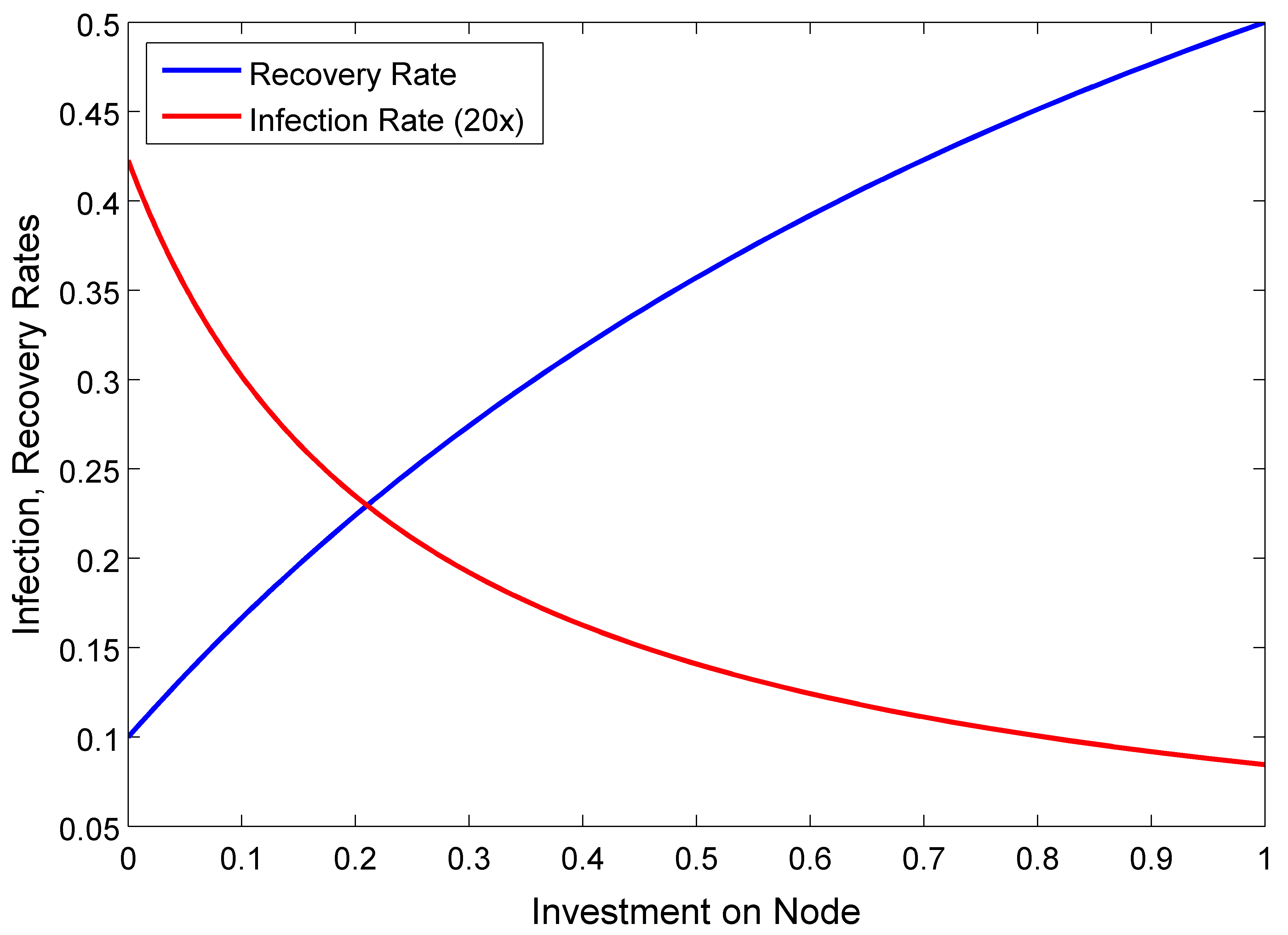
Figure 1.2: Propagation rate (in red, and multiplied by 20, to improve visualization) and recovery rate (in blue) achieved at node $v_{i}$ after an investment on protection (in abscissas) is made on that node.

In this problem, we assume that allocating preventive resources (e.g. vaccines) at a particular airport, scale down the propagation rate of all the incoming links in proportion to the incoming traffic. In other words, we assume that $\beta_{ij}=\beta_{i}a_{ij}$, where $a_{ij}$ is the number of passengers per year (in MPPY) that travel from airport $v_{j}$ to airport $v_{i}$, and $\beta_{i}$ is a scaling factor that depends on the destination airport only. In our simulations, we consider the following cost functions $f_{ij}\left(\beta_{ij}\right)=f\left(\beta_{i}\right)$ and $g_{i}\left(\delta_{i}\right)=g\left(\delta_{i}\right)$, where $f$ and $g$ are the following functions (plotted in Figure 1.2):

$$f_{i}\left(\beta_{i}\right)=\frac{\beta_{i}^{-1}-\bar{\beta}_{i}^{-1}}{\underline{\beta}_{i}^{-1}-\bar{\beta}_{i}^{-1}},\quad g_{i}\left(\delta_{i}\right)=\frac{\left(1-\delta_{i}\right)^{-1}-\left(1-\underline{\delta}_{i}\right)^{-1}}{\left(1-\overline{\delta}_{i}\right)^{-1}-\left(1-\underline{\delta}_{i}\right)^{-1}}.$$ (1.15)

Notice that as we increase the amount invested on vaccines, the propagation rate of that node is reduced from $\bar{\beta}_{i}$ to $\underline{\beta}_{i}$ (red line). Similarly, as we increase the amount invested on antidotes at a node $v_{i}$, the recovery rate grows from $\underline{\delta}_{i}$ to $\bar{\delta}_{i}$ (blue line). Notice that both cost functions present diminishing marginal benefit on investment.

Using the air transportation network and the cost functions specified above, we solve the budget-constrained allocation problem using the geometric programs in Theorems 2. In the left subplot of Figure 1.3, we present a scatter plot with $56$ circles (one circle per airport), where the abscissa of each circle is equal to $g\left(\delta_{i}^{*}\right)$ and the ordinate is $f\left(\beta_{i}^{*}\right)$, namely, the investments on allocation of vaccines and antidotes on the airport at node $v_{i}$, for all $v_{i}\in\mathcal{V}$. We observe an interesting pattern in the allocation of preventive and corrective resources in the network. In particular, we have that in the optimal allocation some airports receive only corrective resources (indicated by circles located on top of the $x$-axis), and some airports receive a mixture of preventive and corrective resources. In the center and right subplots in Fig. 1.3, we compare the distribution of resources with the in-degree and the PageRank centralities of the nodes in the network [51]. In the center subplot, we have a scatter plots where the ordinates represent investments on prevention (red +’s), correction (blue x’s), and total investment (the sum of prevention and correction investments, in black circles) for each airport, while the abscissas are the (weighted) in-degrees of the airports under consideration. We again observe a nontrivial pattern in the allocation of investments for protections. In particular, for airports with incoming traffic less than $4$ MPPY, only corrective resources are needed. Airports with incoming traffic over $4$ MPPY receive both preventive and corrective resources. In the right subplot in Fig. 1.3, we include a scatter plot of the amount invested on prevention and correction for each airport versus its PageRank centrality in the transportation network. We observe that there is a strong correlation between the network centrality measures and the level of investment per node. In particular, there is an almost affine relationship between the total level of investment (black circles in Fig. 1.3, center) and the incoming traffic of an airport. Furthermore, there is a clear piece-wise linear affine relationship between the levels of investment on prevention and correction (Fig. 1.3, left). Similar relationships also hold when comparing the levels of investment versus the Page-Rank centralities in the airport network (Fig. 1.3, right).

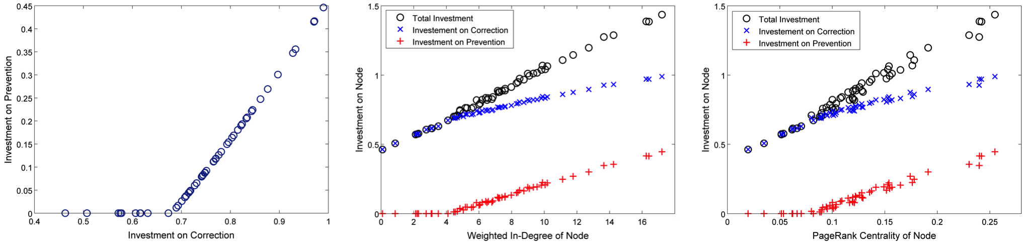
Figure 1.3: Results from the budget-constrained allocation problem. From left to right, we have (a) a scatter plot with the investment on correction versus prevention per node, (b) a scatter plot with the investment on protection per node and the in-degrees, and (c) a scatter plot with the investment on protection per node versus PageRank centralities.

Notice that the above distribution of protection resources correspond to the particular cost functions chosen for our simulations. Changes in these cost functions allow us to observe interesting phenomena in the optimal distribution of protection resources, such as airports with a zero protection assignment at optimality, or a distribution of resources with a negative correlation with centrality measures. For example, it is possible to build cases in which nodes with low centrality (e.g. nodes with low incoming traffic and PageRank) are assigned at optimality a higher level of protection than more central nodes [86].

1.3 Towards a General Framework for Network Protection

The framework presented in this chapter has been recently extended in several directions. In what follows, we briefly describe the following extensions: (i) a generalized framework to cover more realistic epidemic models (beyond SIS), (ii) a novel data-driven framework able to handle network uncertainties, and (iii) an analysis tool that allows us to study non-Poissonian transmission and recovery rates.

1.3.1 Generalized Epidemic Models

In Nowzari et al. [52, 12], the authors recently studied a model of spreading, called the Generalized Susceptible-Exposed-Infected-Vigilant (G-SEIV) model, that generalizes many of the models in the literature, including SIS, SIR, SIRS, SEIR, SEIV, SEIS, and SIV [60, 30]. This model has two two infectious states, called Infected (I) and Exposed (E), that allow us to model human behavioral changes. An individual is in the Exposed state if she is infected and contagious, but not yet aware that she is sick (i.e., in an asymptomatic incubation period). Individuals in the Infected are infected and aware of the disease, which induces a different behavior. For instance, a person knowingly infected with a disease may have much less contact with others, yielding less chance of spreading the infection. The dynamics of this model is described below. The G-SEIV model also includes a Vigilant (V) state, which represents healthy individuals being aware of the disease being spread. Hence, individuals in the Vigilant state are more careful in their social contacts and less likely to be infected.

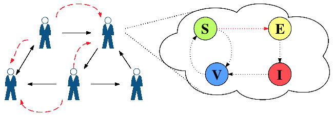
Figure 1.4: Generalized Susceptible-Exposed-Infected-Vigilant model in a network of individuals. (Source of figure: [52]).

Let us denote by $\left[S_{i}(t),E_{i}(t),I_{i}(t),V_{i}(t)\right]^{T}$ the probability vector associated with node $i$ being in each one of these states: Susceptible, Exposed, Infected, or Vigilant, respectively. Using a mean-field approximation, the dynamics of the G-SEIV model can be described as:

$$\dot{S}_{i}(t) =\gamma_{i}V_{i}(t)-{\theta}_{i}S_{i}(t)-S_{i}(t)\left(\sum_{j\in{\mathcal{N}}^{\text{in}}_{i}}{\beta}^{E}_{i}E_{j}(t)+{\beta}^{I}_{i}I_{j}(t)\right)$$

$$\dot{E}_{i}(t) =S_{i}(t)\left(\sum_{j\in{\mathcal{N}}^{\text{in}}_{i}}{\beta}^{E}_{i}E_{j}(t)+{\beta}^{I}_{i}I_{j}(t)\right)-\varepsilon_{i}E_{i}(t)$$

$$\dot{I}_{i}(t) =\varepsilon_{i}E_{i}(t)-{\delta}_{i}I_{i}(t)$$ (1.16)

$$\dot{V}_{i}(t) ={\delta}_{i}I_{i}(t)+{\theta}_{i}S_{i}(t)-\gamma_{i}V_{i}(t).$$

Using nonlinear analysis techniques, Nowzari et al. derived the following necessary and sufficient condition for the disease to die out exponentially fast:

Theorem 1.3.1.

(Conditions for stability of disease-free equilibrium) The disease-free equilibrium of the G-SEIV model is globally exponentially stable if and only if the following matrix,

$$Q=\left[\begin{array}[]{cc}TB^{E}A_{\mathcal{G}}-E&TB^{I}A_{\mathcal{G}}\\ E&-D\end{array}\right].$$ (1.19)

is Hurwitz, where $B^{E}=\operatorname{diag}\left(\beta^{E}\right),B^{I}=\operatorname{diag}\left(\beta^{I}\right),D=\operatorname{diag}\left(\delta\right),E=\operatorname{diag}\left(\varepsilon\right),$ $T=\operatorname{diag}\left(\frac{\gamma}{\theta+\gamma}\right)$

The above result can be used to mitigate, or eliminate completely, the spreading of the disease. In [52], the authors considered three types of resources are available to control the disease: corrective resources (e.g., antidotes), preventative resources (e.g., vaccines), and preemptive resources (e.g., awareness campaigns and/or limiting traffic). Under mild conditions on the cost functions of these resources, the authors were able to bound the rate of spreading of the undesired disease.

1.3.2 Data-Driven Allocation

Although current vaccination strategies assume full knowledge about the network structure and spreading rates, in most practical applications, this information is only partially known. To elaborate on this point, let us consider the following setup. Assume that each node in the network represents subpopulations (e.g., city districts) connected by edges that are determined by commuting patterns between districts. In practice, one can use traffic information and geographical proximity to infer the existence of an edge connecting districts. For example, in Fig. 1.5, we represent such a network for those districts in West Africa affected by the 2014 Ebola outbreak. On the other hand, it is very challenging to use this information to estimate the contact rates between subpopulations. Inspired by this example, we considered in [28] a networked SIS model taking place in a contact network of unknown contact rates. To extract information about these unknown rates, we assumed that we have access to time series describing the evolution of the spreading process observed from a collection of sensor nodes during a finite time interval.

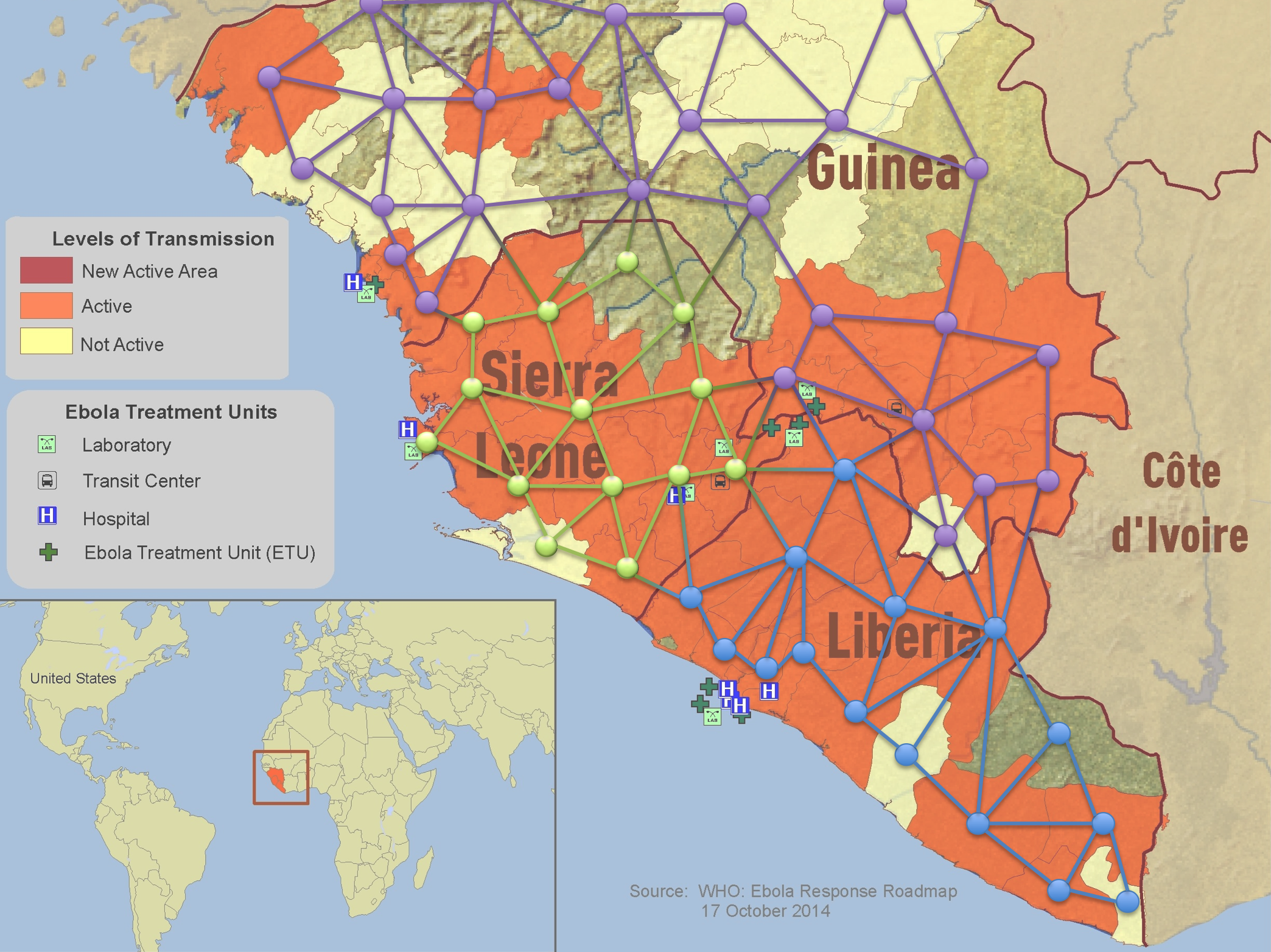
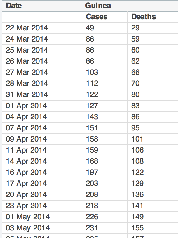
Figure 1.5: Network of districts in West Africa affected by the 2014 Ebola outbreak. (Source: WHO)

In contrast to current network identification heuristics, in which a single network is identified to explain the observed data, the authors in [28] developed a robust optimization framework in which an uncertainty set containing all networks that are coherent with empirical observations is defined. This characterization of the uncertainty set of networks is tractable in the context of conic geometric programming, recently proposed by Chandrasekaran and Shah [15]. In this context, the authors were able to efficiently find the optimal allocation of resources to control the worst-case spread that can take place in the uncertainty set of networks. In order to extract information about the contact rates, the authors considered two different sources of information that are usually available in epidemiological problems. These sources can be classified as (i) prior information about the network topology and parameters of the disease, and (ii) empirical observations about the spreading dynamics. In particular, one can consider the following pieces of prior information:

1. Assume that the sparsity pattern of the contact matrix $B_{\mathcal{G}}$ is given, although its entries are unknown. This piece of information may be inferred from geographical proximity, commuting patterns, or the presence of transportation links connecting subpopulations.

2. Assume that upper and lower bounds on the spreading rates associated to each edge, i.e., $\beta_{ij}\in\left[\underline{\beta}_{ij},\overline{\beta}_{ij}\right]$, for all $\left(i,j\right)\in\mathcal{E}$, are available. This could be inferred from traffic densities and subpopulation sizes.

3. In practice, each district contains a large number of individuals. Therefore, one can use the average recovery rate in the absence of vaccination as an estimation of the nodal recovery rate. We denote this ‘natural’ recovery rate by $\delta_{i}^{0}$, and assume it to be known.

Apart from these pieces of prior information, the authors in [28] also assumed that they had access to partial observations about the evolution of the spread over a finite time interval. In particular, assume that we observe the dynamics of the disease for $t\in\left[0,T\right]$ from a collection of sensor nodes $\mathcal{V}_{S}\subseteq\mathcal{V}$. Based on these pieces of information, one can define an uncertainty set that contains all contact matrices $B_{\mathcal{G}}$ consistent with both empirical observations and prior knowledge. This set contains those contact matrices $B_{\mathcal{G}}$ such that the transmission rates $\{\beta_{ij}\}$ are consistent with the disease dynamics.

In order to eradicate the disease at the fastest rate possible, the authors in [28] considered the following control problem:

Problem 3.

(Data-driven optimal allocation) Assume the following pieces of information about a viral spread are given:

(i) prior information about the state matrix (as described in P1–P3);

(ii) a finite (and possibly sparse) data series representing partial evolution of the spread over a set of sensor nodes $\mathcal{V}_{S}\subseteq\mathcal{V}$ during the time interval $t\in\left[T\right]$ (i.e., $\mathcal{D}$ in (LABEL:eq:Data_Series));

(iii) a set of vaccine cost functions $g_{i}$ for all $i\in\mathcal{V}_{C}$, and a range of feasible recovery rates $\left[\underline{\delta}_{i}^{c},\overline{\delta}_{i}^{c}\right]$ such that $1-\delta_{i}^{0}=\overline{\delta}_{i}^{c}\geq\delta_{i}^{c}\geq\underline{\delta}_{i}^{c}>0$;

(iv) a fixed budget $C>0$ to be allocated throughout a set of control nodes in $\mathcal{V}_{C}\subseteq\mathcal{V}$, so that $\sum_{i\in\mathcal{V}_{C}}g_{i}(\delta_{i}^{c})\leq C$.

Find the cost-constrained allocation of control resources to eradicate the disease at the fastest possible exponential rate, measured as $\rho(M(B_{\mathcal{G}},\mathbf{d}^{c}))$, over the uncertainty set $\Delta_{B_{\mathcal{G}}}$ of contact matrices coherent with prior knowledge and the observations in $\mathcal{D}$.

From the perspective of optimization, Problem 3 is equivalent to finding the optimal allocation of resources to minimize the worst-case (i.e., maximum possible) decay rate $\rho(M(B_{\mathcal{G}},\mathbf{d}^{c}))$ for all $B_{\mathcal{G}}\in\Delta_{B_{\mathcal{G}}}$. In Han et al. [28], a robust optimization framework was developed to solve this problem, even in the presence of sparse observations.

1.3.3 Non-Poissonian Rates

The vast majority of spreading models over networks assume exponentially distributed transmission and recovery rates. In contrast, empirical observations indicate that most real-world spreading processes do not satisfy this assumption [48, 47, 46]. For example, the transmission rates of human immunodeficiency viruses present a distribution far from exponential [6]. In the context of online social networks, empirical studies show that the rate of spreading of information follow (approximately) a log-normal distribution [43, 78].

There are only a few results available for analyzing spreading processes over networks with non-exponential transmission and recovery rates. The experimental study in [80] confirmed the dramatic effect that non-exponential rates can have on the speed of spreading, as well as on the epidemic threshold. In [34], an analytically solvable (although rather simplistic) model of spreading with non-exponential rates was proposed. An approximate criterion for epidemic eradication over graphs with general transmission and recovery times based on asymptotic approximations was proposed in [13].

In the recent work [54, 56], the authors propose an alternative approach to analyze general transmission and recovery rates using phase-type distributions. In particular, they derive conditions for disease eradication using transmission and recovery times that follow phase-type distributions (see, e.g., [2]). The class of phase-type distributions is dense in the space of positive-valued distributions [19], hence, it can be used to theoretically analyze arbitrary transmission and recovery rates. Furthermore, there are efficient algorithms to compute the parameters of a phase-type distributions to approximate any given distribution [2]. The key tool in this analysis is a vectorial representations proposed in [11], which can be used to represent phase-type distributions.

1.4 Comparisons with Common Heuristics

Usual approaches to distribute protection resources in a network of agents susceptible to cascade failures are heuristics based on network centrality measures [51]. As in the optimal framework presented in the previous section, much of the literature uses a bio-inspired epidemic models when studying harmful process with the ability to spread between interconnected agents. The main idea behind heuristic protection strategies is to rank agents according to different measures of importance based on their location in the network and greedily distribute protection resources based on each agents rank. For example, Cohen et al. [18] proposed a simple protection strategy called acquaintance immunization policy in which the most connected node of a randomly selected node is given protective resources. This strategy was proved to be much more efficient than random allocation of protective resources. Hayashi et al. [29] proposed a simple heuristic called targeted immunization consisting on greedily choosing nodes with the highest degree (number of connections) in scale-free graphs. Chung et at. [17] studied a greedy heuristic protection strategy based on the PageRank vector of the contact graph. Tong et al. [75] and Giakkoupis et al. [25] proposed greedy heuristics based on protecting those agents that induce the highest drop in the dominant eigenvalue of the contact graph. Recently, Prakash et al. [3] proposed several greedy heuristics to contain harmful cascades in directed networks when nodes can be partially protected (instead of completely removed, as assumed in previous work). These heuristics, as those in [75, 29], are based on eigenvalue perturbation analysis.

The heuristic methods in the literature are designed for a single resource type, predominantly the protective resources. A simplified variant of the budget-constrained allocation problem is presented with only protection-type resources in order to compare the optimal solution with heuristic solutions.

Problem 4.

The Network Protection Problem is given by

$$\max_{\beta,\varepsilon} \varepsilon$$

$$s.t. \Re[\lambda_{1}(BA-\delta I)]\leq-\varepsilon$$

$$\sum_{i=1}^{n}f(\beta_{i})\leq C$$

$$\underline{\beta}\leq\beta_{i}\leq\bar{\beta}\qquad\forall i\in V.$$

1.4.1 Greedy, Centrality Based Strategies

Definition 1.4.1.

Extract the effective objective in Problem 4 which is induced by the epigraph form. Define

$$\varepsilon({\beta})=-\Re[\lambda_{1}(BA-\delta I)]$$ (1.20)

where $B=\hbox{diag}(\beta)$ for any feasible resource allocation $\beta$.

Monotonicity and continuity of the function $\varepsilon({\beta})$ guarantee that fixing any feasible $\beta$ and maximizing over $\varepsilon$ always causes the constraint $\Re[\lambda_{1}(BA-\delta I)]\leq-\varepsilon$ to become tight. At the optimal point $(\beta^{*},\varepsilon^{*})$ of Problem 4 satisfies

$$\varepsilon^{*}=-\Re[\lambda_{1}(\hbox{diag}(\beta^{*})A-\delta I)].$$

When solving the resource allocation $\beta$, $\varepsilon(\beta)$ is treated as the effective objective in Problem 4.

Definition 1.4.2.

Define the efficiency of a feasible resource allocation $\beta$ as

$$Q(\beta)=\frac{\varepsilon(\beta)-\varepsilon(\bar{\beta})}{\varepsilon(\beta^{*})-\varepsilon(\bar{\beta})}\in[0,1]$$ (1.21)

where $\beta^{*}$ is a resource allocation achieving the maximum in Problem 4.

The effective objective $\varepsilon(\beta)$ and the costs functions $f(\beta_{i})$ are monotonically non-increasing in the resource allocations $\beta_{i}$ at each node, therefore $\bar{\beta}$ trivially achieves the minimum over the set of feasible resource allocations $\beta$.

Definition 1.4.3.

Let $v$ be a centrality vector. Given a budget sufficient to completely protect $k$ nodes: $C=kf(\underline{\beta})$, the greedy protection strategy $\widehat{\beta}_{v}$ is to completely protect $k$ nodes with the highest values in $v$. Define the protection fraction: $r=k/N$ where $N=n+m$ is the the total number of nodes.

Common centrality measures used for heuristics are degree and eigenvector centrality, [29]. Page rank centrality is used as in place of eigenvector centrality in the case of general digraphs, [17]. While Page rank depends on a parameter $\alpha$, we drop the $\alpha$ from our notation because our results hold for the whole family of Page rank vectors generated by non-trivial choices of $\alpha\in(0,1)$.

Theorem 1.4.1.

Given the Network Protection Problem defined in Problem 4, with budget $C$, there exists a network $G$ satisfying

$$Q(\widehat{\beta}_{DEG})=Q(\widehat{\beta}_{PR})=0$$

where $r\in(0,1)$ is the fraction of nodes that can be fully protected.

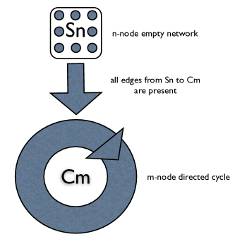
Figure 1.6: We construct the network $G$ to prove theorem 1.4.1.

Theorem 1.4.1 is based on a worst case graph construction as shown in Fig. 1.6. Define the subgraph $C_{m}$ as an $m$ node directed cycle, $S_{n}$ as an $n$ node empty network and the there are edges from all nodes $i\in S_{n}$ to all nodes $j\in C_{m}$. Formally, the edge set is given by

$$(i,j)\in\mathcal{E}\hbox{ if any of }\left\{\begin{array}[]{l}i\in S_{n},j\in C_{m}\\ i,j=i+1\in C_{m}\\ i=m+n,j=n+1\in C_{m}\end{array}\right.$$ (1.22)

and in all other cases $(i,j)\not\in\mathcal{E}$. All weights are given by $\mathcal{W}(i,j)=1$ for $(i,j)\in\mathcal{E}$. Given a vaccination fraction $r$, the size of the subgraphs $C_{m}$ and $S_{n}$ must satisfy $m>n+2$ and $rN<n$ in order to generate a network for which greed heuristics have zero efficiency. Such $m$ and $n$ exist for any $r\in(0,1)$ but the networks required become very large as $r\rightarrow 1$.

The weakly connected network $G$ results in a spreading process dominated by the nodes in $C_{m}$ even though nodes in $S_{n}$ have larger centralities. A generalization of Theorem 1.4.1, which builds a strongly connected network with arbitrarily small efficiency can be found in [86].

Remark 1.4.1.

The proof of Theorem 1.4.1 makes use of a constructive example for the centrality measures which identify nodes which are the most likely to fail: (a) out degree and (b) Page rank with a random walk defined as moving up the edges. If one uses centrality measures which identify nodes which would be the most potent seeds such as (c) in degree or (d) Page rank computed using a random walk that flows down the edges, one can construct an alternative $G$ by simply reversing the direction of the edges from $S_{n}$ to $C_{m}$. Using this alternative network, one can reproduce Theorem 1.4.1 for (c) and (d).

1.4.2 Greedy Heuristics and Workstation Protection

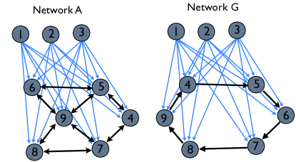
Figure 1.7: Network G with vertices $S_{3}=\{1,2,3\}$ and $C_{6}=\{4,5,\dots,9\}$ satisfies the conditions for the counter example network defined in Theorem 1.4.1. In Network A the subgraph on $C_{6}$ is relaxed to be less structured for demonstration purposes.

Consider a simple application in which such a worst case network might arise naturally: nodes are computers belonging to individuals in a work environment. Edges indicate access to files on another persons computer.
Each workstation in $C_{m}$ is an element in the cyber layer, paired with one or more plants in the physical layer. Workstations in $S_{n}$ exist only in the cyber layer and belong to a group of administrators who can access files on all workstations in $C_{m}$.
Workers have limited access to each others files, but do not have access to files on the administrator’s computers. A virus may spread when an uninfected computer accesses an infected computer. It is assumed that an infected workstation cannot adequately control its associated plant which leads to physical layer failures. Protection resources take the form of antivirus software with updates on a variable time interval, software updated more frequently providing a smaller infection rate $\beta$ but updates incurring a greater cost $f(\beta)$. The cost function

$$f(\beta_{i})=\frac{\underline{\beta}(\frac{\bar{\beta}}{\beta_{i}}-1)}{\bar{\beta}-\underline{\beta}}$$ (1.23)

is chosen to satisfy $f(\bar{\beta})=0$, $f(\underline{\beta})=1$ and $f(\beta)\propto 1/\beta$. This allows us to choose capacity $C$ equal to the number of nodes we wish to be able to allocate maximum protection. In our example the infection rate with outdated anti-virus software is $\bar{\beta}=.5$ while the maximum update rate achieves an infection rate of $\underline{\beta}=.01$. Choosing a budget of $C=3$ for a network with $n=3$ and $m=6$ (such as in G or A shown in Fig. 1.7), the fraction of nodes that can be maximally protected is $r=1/3$. An infected machine has recovery rate $\delta=0.3$, based on curative resources in the form of IT staff, which are uniformly available.

In the example, four heuristic algorithms based on greedily allocating resources with respect to centrality measures are considered. The centrality measures are out degree, total degree, Page rank with $\alpha=.1$ and symmetrized Page rank with $\alpha=.1$. Symmetrized Page rank is computed by allowing the random walk move over a directed edge in either direction. The worst case networks are products of extreme asymmetry between $C_{m}$ and $S_{n}$, the symmetric centrality measure show that even symmetric centrality measure don’t overcome the potential for arbitrarily poor behavior.

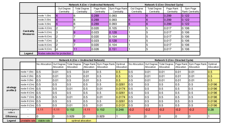
Figure 1.8: (Top) A variety of centrality measures are used as the basis for greedy algorithms, these measures are reported for the Networks A and G. (Bottom) The allocation strategies tested are detailed, their exponential convergence rate bounds $\varepsilon$ and their efficiencies are reported for comparison purposes. For the case of the counter example network G, none of the greedy type algorithms yield a stable convergence rate.

In Fig. 1.8 the top table shows all of the centrality vectors for the example problem in the networks $A$ and $G$. The network $G$ is the network constructed in our analytical proofs. The network $A$ is an example of a less structured employee collaboration network which we include to demonstrate two points: (i) our constructed network G is not unique and (ii) symmetrizing heuristics are less fragile than heuristics that respect edge direction.

In $G$ and $A$ the out degree and Page rank heuristics allocate all resources to the admins, $S_{n}$. This is ineffective because even though the admins are the most likely to become infected the worker group, $C_{m}$ cannot access their files and become infected. Furthermore, the failure of admin workstation does not lead directly to physical layer failures. Fig. 1.8 (bottom) shows the infection rate profiles generated by the various heuristics and the optimal solution. A strategy is ineffective if the convergence rate epsilon is negative because this corresponds to unstable dynamics, where the computer virus is spreading faster than the IT staff can repair workstations. The result is a complete failure to consistently control any of the plants in the physical layer of the system.

1.5 Conclusions

We have studied the problem of allocating protection resources in weighted, directed networks to contain spreading processes, such as the propagation of viruses in computer networks, cascading failures in complex technological networks, or the spreading of an epidemic in a human population. We have considered two types of protection resources: (i) Preventive resources able to ‘immunize’ nodes against the spreading (e.g. vaccines), and (ii) corrective resources able to neutralize the spreading after it has reached a node (e.g. antidotes). We assume that protection resources have an associated cost and have then studied the budget-constrained allocation problem, in which we find the optimal allocation of resources to contain the spreading given a fixed budget. We have solved this optimal resource allocation problem in weighted and directed networks of nonidentical agents in polynomial time using Geometric Programming (GP). Furthermore, the framework herein proposed allows simultaneous optimization over both preventive and corrective resources, even in the case of cost functions being node-dependent.

We have illustrated our approach by designing an optimal protection strategy for a real air transportation network. We have limited our study to the network of the world’s busiest airports by passenger traffic. For this transportation network, we have computed the optimal distribution of protecting resources to contain the spread of a hypothetical world-wide pandemic. Our simulations show that the optimal distribution of protecting resources follows nontrivial patterns that cannot, in general, be described using simple heuristics based on traditional network centrality measures.

We then presented the following recent extensions on this work: (i) a generalized framework to cover more realistic epidemic models, (ii) a novel data-driven framework able to handle network uncertainties, and (iii) an analysis tool that allows us to study non-Poissonian transmission and recovery rates. We concluded this chapter with a comparison between our results and common heuristics used in the literature.

Exercises

Consider the following three networks with $n$ nodes:

Answer the following questions:

Question 1. Compute the largest eigenvalue of the adjacency matrices of the graphs in figures (a), (b) and (c) as a function of $n$.

Question 2. Consider the SIS model of spreading with $\beta=0.1$ and $n=100$. For what values of $\delta$ does an epidemics die out in for each one of the three networks above? (Reminder: The epidemic dies out when $\lambda_{1}<\delta/\beta$).

Question 3. Imagine you work for a health agency responsible for controlling an epidemic taking place in the above networks. Assume you can tune the spreading rates of the edges within a feasible interval $[\underline{\beta},\overline{\beta}]$. Assume the cost associated with tuning $\beta$ is given by $f_{ij}(\beta)=1/\beta$. Write the associated optimization problem for each one of the above networks. (Hint: Your answer should look like equations 1.5–1.8).

Question 4. Transform the optimization problem in Question 3 into a standard geometric program. (Hint: Your answer should look like equations 1.11–1.14).

Question 5. Implement the geometric program from Question 4 using MATLAB’s CVX Toolbox [27].

Bibliography

- [1] Anderson, R. M., May, R. M., and Anderson, B. Infectious Diseases of Humans: Dynamics and Control, vol. 28. Wiley, 1992.
- [2] Asmussen, S., Nerman, O., and Olsson, M. Fitting phase-type distributions via the em algorithm. Scandinavian Journal of Statistics (1996), 419–441.
- [3] B. Aditya Prakash, L. Adamic, T. I. H. T., and Faloutsos, C. Fractional immunization in networks. Proc. SDM (2013).
- [4] Bailey, N. The mathematical theory of infectious diseases and its applications. Charles Griffin & Company Ltd., 1975.
- [5] Biggs, N. Algebraic Graph Theory. Cambridge University Press, 1993.
- [6] Blythe, S., and Anderson, R. Variable infectiousness in hfv transmission models. Mathematical Medicine and Biology 5, 3 (1988), 181–200.
- [7] Borgs, C., Chayes, J., Ganesh, A., and Saberi, A. How to distribute antidote to control epidemics. Random Structures & Algorithms 37, 2 (2010), 204–222.
- [8] Boyd, S., Kim, S.-J., Vandenberghe, L., and Hassibi, A. A tutorial on geometric programming. Optimization and engineering 8, 1 (2007), 67–127.
- [9] Boyd, S., and Vandenberghe, L. Convex optimization. Cambridge university press, 2004.
- [10] Breda, D., Diekmann, O., de Graaf, W. F., Pugliese, A., and Vermiglio, R. On the formulation of epidemic models (an appraisal of Kermack and McKendrick). Journal of Biological Dynamics 6, 2 (2012), 103–117.
- [11] Brockett, R. Optimal control of observable continuous time markov chains. In Decision and Control, 2008. CDC 2008. 47th IEEE Conference on (2008), IEEE, pp. 4269–4274.
- [12] C. Nowzari, V. P., and Pappas, G. Analysis and control of epidemics: A survey of spreading processes on complex networks. IEEE Transactions on Network Science and Engineering 36, 1 (2016), 26–46.
- [13] Cator, E., Van de Bovenkamp, R., and Van Mieghem, P. Susceptible-infected-susceptible epidemics on networks with general infection and cure times. Physical Review E 87, 6 (2013), 062816.
- [14] Chakrabarti, D., Wang, Y., Wang, C., Leskovec, J., and Faloutsos, C. Epidemic thresholds in real networks. ACM Transactions on Information and System Security 10, 4 (2008), 1–26.
- [15] Chandrasekaran, V., and Shah, P. Conic geometric programming. In Information Sciences and Systems (CISS), 2014 48th Annual Conference on (2014), IEEE, pp. 1–4.
- [16] Chen, X., and Preciado, V. Optimal coinfection control of competitive epidemics in multilayer networks. Proceedings of the IEEE Conference on Decision and Control (2014).
- [17] Chung, F., Horn, P., and Tsiatas, A. Distributing antidote using pagerank vectors. Internet Mathematics 6, 2 (2009), 237–254.
- [18] Cohen, R., Havlin, S., and Ben-Avraham, D. Efficient immunization strategies for computer networks and populations. Physical Review Letters 91, 24 (2003), 247901.
- [19] Cox, D. R. A use of complex probabilities in the theory of stochastic processes. In Mathematical Proceedings of the Cambridge Philosophical Society (1955), vol. 51, Cambridge Univ Press, pp. 313–319.
- [20] Domínguez-García, A. D. An integrated methodology for the performance and reliability evaluation of fault-tolerant systems. PhD thesis, Massachusetts Institute of Technology, 2007.
- [21] Funk, S., Gilad, E., and Jansen, V. A. A. Endemic disease, awareness, and local behavioural response. Journal of Theoretical Biology 264, 2 (2010), 501–509.
- [22] Ganesh, A., Massoulie, L., and Towsley, D. The effect of network topology on the spread of epidemics. In IEEE INFOCOM 2005 (2005), vol. 2, pp. 1455–1466.
- [23] Garetto, M., Gong, W., and Towsley, D. Modeling malware spreading dynamics. In IEEE INFOCOM 2003 (2003), vol. 3, pp. 1869–1879.
- [24] Garetto, M., Gong, W., and Towsley, D. Modeling malware spreading dynamics. In INFOCOM Joint Conference of the IEEE Computer and Communications Societies (San Francisco, CA, 2003), pp. 1869–1879.
- [25] Giakkoupis, G., Gionis, A., Terzi, E., and Tsaparas, P. Models and algorithms for network immunization. Tech. rep., Technical Report C-2005-75, Department of Computer Science, University of Helsinki, 2005.
- [26] Gourdin, E., Omic, J., and Van Mieghem, P. Optimization of network protection against virus spread. In 8th International Workshop on the Design of Reliable Communication Networks (2011), pp. 86–93.
- [27] Grant, M., Boyd, S., and Ye, Y. Cvx: Matlab software for disciplined convex programming, 2008.
- [28] Han, S., Preciado, V., Nowzari, C., and Pappas, G. Data-driven allocation of vaccines for controlling epidemic outbreaks. IEEE Transactions on Network Science and Engineering (2015).
- [29] Hayashi, Y., Minoura, M., and Matsukubo, J. Recoverable prevalence in growing scale-free networks and the effective immunization. arXiv preprint cond-mat/0305549 (2003).
- [30] Hethcote, H. W. The mathematics of infectious diseases. SIAM Review 42, 4 (2000), 599–653.
- [31] Hethcote, H. W., Stech, H. W., and van den Driessche, P. Stability analysis for models of diseases without immunity. Journal of Mathematical Biology 13, 2 (1981), 185–198.
- [32] Hikal, M. M. Dynamic properties for a general SEIV epidemic model. SIAM Review 2, 1 (2014), 26–36.
- [33] Iyer, B. R., Donatiello, L., and Heidelberger, P. Analysis of performability for stochastic models of fault-tolerant systems. Computers, IEEE Transactions on 100, 10 (1986), 902–907.
- [34] Jo, H.-H., Perotti, J. I., Kaski, K., and Kertész, J. Analytically solvable model of spreading dynamics with non-poissonian processes. Physical Review X 4, 1 (2014), 011041.
- [35] Keeling, M. J., and Rohani, P. Modeling Infectious Diseases in Humans and Animals. Princeton University Press, 2007.
- [36] Kephart, J. O., and White, S. R. Directed-graph epidemiological models of computer viruses. In IEEE Symposium on Research in Security and Privacy (Oakland, CA, 1991), pp. 343–359.
- [37] Kephart, J. O., and White, S. R. Measuring and modeling computer virus prevalence. In IEEE Symposium on Research in Security and Privacy (Oakland, CA, 1993), pp. 2–15.
- [38] Khanafer, A., Ba?ar, T., and Gharesifard, B. Stability of epidemic models over arbitrary graphs: A positive systems approach. Automatica, submitted (2014).
- [39] Kiss, I. Z., Cassell, J., Recker, M., and Simon, P. L. The impact of information transmission on epidemic outbreaks. Mathematical Biosciences 225, 1 (2010), 1–10.
- [40] Korobeinikov, A., and Wake, G. C. Lyapunov functions and global stability for SIR, SIRS, and SIS epidemiological models. Applied Mathematics Letters 15, 8 (2002), 955–960.
- [41] Lahrouz, A., Omari, L., and Kiouach, D. Global analysis of a deterministic and stochastic nonlinear SIRS epidemic model. Nonlinear Analysis: Modelling and Control 16, 1 (2011), 59–76.
- [42] Lajmanovich, A., and Yorke, J. A. A deterministic model for gonorrhea in a nonhomogeneous population. Mathematical Biosciences 28, 3 (1976), 221–236.
- [43] Lerman, K., and Ghosh, R. Information contagion: An empirical study of the spread of news on digg and twitter social networks. ICWSM 10 (2010), 90–97.
- [44] Leskovec, J., Adamic, L. A., and Huberman, B. A. The dynamics of viral marketing. ACM Transactions on the Web (TWEB) 1, 1 (2007), 5.
- [45] Li, J., Yang, Y., and Zhou, Y. Global stability of an epidemic model with latent stage and vaccination. Nonlinear Analysis: Real World Applications 12, 4 (2011), 2163–2173.
- [46] Lloyd, A. L. Destabilization of epidemic models with the inclusion of realistic distributions of infectious periods. Proceedings of the Royal Society of London B: Biological Sciences 268, 1470 (2001), 985–993.
- [47] Lloyd, A. L. Realistic distributions of infectious periods in epidemic models: changing patterns of persistence and dynamics. Theoretical population biology 60, 1 (2001), 59–71.
- [48] LOG, O. Log-normal distributions across the sciences: Keys and clues. BioScience 51, 5 (2001).
- [49] Meyer, C. Matrix analysis and applied linear algebra. SIAM, 2000.
- [50] N. Watkins, C. Nowzari, V. P., and Pappas, G. Optimal resource allocation for competitive spreading processes on bilayer networks. IEEE Transactions on Control of Network Systems (in press.).
- [51] Newman, M. Networks: An introduction. Cambridge University Press, 2010.
- [52] Nowzari, C., Preciado, V., and Pappas, G. Optimal resource allocation in generalized epidemic models. IEEE Transactions on Control of Networked Systems (in press).
- [53] Ogura, M., and Preciado, V. Disease spread over randomly switched large-scale networks. Proceedings of the IEEE American Control Conference (2015).
- [54] Ogura, M., and Preciado, V. Spreading processes over networks with phase-type transmission and recovery times. arXiv preprint arXiv:1502.07384v1 (2015).
- [55] Ogura, M., and Preciado, V. Epidemic processes over adaptive state-dependent networks. Physical Review E 93 (2016).
- [56] Ogura, M., and Preciado, V. Spreading processes with general transmission and recovery times. arXiv 1606.08518 (2016).
- [57] Ogura, M., and Preciado, V. Stability of spreading processes over time-varying large-scale networks. IEEE Transactions on Network Science and Engineering 3, 1 (2016), 44–57.
- [58] Perra, N., Balcan, D., Gonasalves, B., and Vespignani, A. Towards a characterization of behavior-disease models. PLoS ONE 6, 8 (Aug. 2011), e23084.
- [59] Poletti, P., Caprile, B., Ajelli, M., Pugliese, A., and Merler, S. Spontaneous behavioural changes in response to epidemics. Journal of Theoretical Biology 260, 1 (2009), 31–40.
- [60] Prakash, B. A., Chakrabarti, D., Faloutsos, M., Valler, N., and Faloutsos, C. Got the flu (or mumps)? check the eigenvalue! arXiv:1004.0060 (2010).
- [61] Preciado, V., Darabi Sahneh, F., and Scoglio, C. A convex framework for optimal investment on disease awareness in social networks. In IEEE Global Conference on Signal and Information Processing (2013), pp. 851–854.
- [62] Preciado, V., Draief, M., and Jadbabaie, A. Structural analysis of viral spreading processes in social and communication networks using egonets. arXiv preprint arXiv:1209.0341 (2013).
- [63] Preciado, V., and Jadbabaie, A. Moment-based analysis of spreading processes from network structural information. IEEE Transactions on Automatic Control 21, 2 (2013), 373–382.
- [64] Preciado, V., and Zargham, M. Traffic optimization to control epidemic outbreaks in metapopulation models. In IEEE Global Conference on Signal and Information Processing (2013), pp. 847–850.
- [65] Preciado, V., Zargham, M., Enyioha, C., Jadbabaie, A., and Pappas, G. Optimal vaccine allocation to control epidemic outbreaks in arbitrary networks. In IEEE Conference on Decision and Control (2013).
- [66] Preciado, V., Zargham, M., Enyioha, C., Jadbabaie, A., and Pappas, G. Optimal resource allocation for network protection against spreading processes. IEEE Transactions on Control of Network Systems 1, 1 (March 2014), 99–108.
- [67] Preciado, V. M., and Jadbabaie, A. Spectral analysis of virus spreading in random geometric networks. pp. 4802–4807.
- [68] Preciado, V. M., Zargham, M., and Sun, D. A convex framework to control spreading processes in directed networks. In Information Sciences and Systems (CISS), 2014 48th Annual Conference on (March 2014), pp. 1–6.
- [69] Preciado, V. M., Zargham, M., and Sun, D. Traffic control for network protection against spreading processes. In Conference on Information Sciences and Systems (Princeton, NJ, 2014).
- [70] Ramirez-Llanos, E., and Martinez, S. A distributed algorithm for virus spread minimization. pp. 184–189.
- [71] Rausand, M., and Høyland, A. System reliability theory: models, statistical methods, and applications, vol. 396. John Wiley & Sons, 2004.
- [72] Reibman, A. L., and Veeraraghavan, M. Reliability modeling: An overview for system designers. Computer 24, 4 (1991), 49–57.
- [73] Roy, S., Xue, M., and Das, S. Security and discoverability of spread dynamics in cyber-physical networks. IEEE Transactions on Parallel and Distributed Systems 23, 9 (2012), 1694–1707.
- [74] Schneider, C., Mihaljev, T., Havlin, S., and Herrmann, H. Suppressing epidemics with a limited amount of immunization units. Physical Review E 84, 6 (2011), 061911.
- [75] Tong, H., Prakash, B. A., Tsourakakis, C., Eliassi-Rad, T., Faloutsos, C., and Chau, D. H. On the vulnerability of large graphs. In Data Mining (ICDM), 2010 IEEE 10th International Conference on (2010), IEEE, pp. 1091–1096.
- [76] van den Driessche, P., and Watmourgh, J. Reproduction numbers and sub-threshold endemic equilibria for compartmental models of disease transmission. Mathematical Biosciences 180, 1-2 (2002), 29–48.
- [77] Van Mieghem, P. Performance analysis of communications networks and systems. Cambridge University Press, 2006.
- [78] Van Mieghem, P., Blenn, N., and Doerr, C. Lognormal distribution in the digg online social network. The European Physical Journal B-Condensed Matter and Complex Systems 83, 2 (2011), 251–261.
- [79] Van Mieghem, P., Omic, J., and Kooij, R. Virus spread in networks. IEEE/ACM Transactions on Networking 17, 1 (2009), 1–14.
- [80] Van Mieghem, P., and Van de Bovenkamp, R. Non-markovian infection spread dramatically alters the susceptible-infected-susceptible epidemic threshold in networks. Physical review letters 110, 10 (2013), 108701.
- [81] Wan, Y., Roy, S., and Saberi, A. Network design problems for controlling virus spread. pp. 3925–3932.
- [82] Wan, Y., Roy, S., and Saberi, A. Designing spatially heterogeneous strategies for control of virus spread. IET Systems Biology 2, 4 (2008), 184–201.
- [83] Wang, C., Knight, J. C., and Elder, M. C. On computer viral infection and the effect of immunization. In Proceedings of the 16th Annual Computer Security Applications Conference (New Orleans, LA, 2000), pp. 246–256.
- [84] Wang, Y., Chakrabarti, D., Wang, C., and Faloutsos, C. Epidemic spreading in real networks: An eigenvalue viewpoint. In Proc. 22nd Int. Symp. Reliable Distributed Systems (2003), pp. 25–34.
- [85] Watkins, N., Nowzari, C., Preciado, V., and Pappas, G. Optimal resource allocation for competing epidemics over arbitrary networks. Proceedings of the IEEE American Control Conference (2015).
- [86] Zargham, M., and Preciado, V. Worst-case scenarios for greedy, centrality-based network protection strategies. In Conference on Information Sciences and Systems (2014).
- [87] Zargham, M., and Preciado, V. M. Worst-case scenarios for greedy, centrality-based network protection strategies. In Conference on Information Sciences and Systems (Princeton, NJ, 2014).