Safe Leads and Lead Changes in Competitive Team Sports

Abstract

We investigate the time evolution of lead changes within individual games of competitive team sports. Exploiting ideas from the theory of random walks, the number of lead changes within a single game follows a Gaussian distribution. We show that the probability that the last lead change and the time of the largest lead size are governed by the same arcsine law, a bimodal distribution that diverges at the start and at the end of the game. We also determine the probability that a given lead is “safe” as a function of its size $L$ and game time $t$. Our predictions generally agree with comprehensive data on more than 1.25 million scoring events in roughly 40,000 games across four professional or semi-professional team sports, and are more accurate than popular heuristics currently used in sports analytics.

I Introduction

Competitive team sports, including, for example, American football, soccer, basketball and hockey, serve as model systems for social competition, a connection that continues to foster intense popular interest. This passion stems, in part, from the apparently paradoxical nature of these sports. On one hand, events within each game are unpredictable, suggesting that chance plays an important role. On the other hand, the athletes are highly skilled and trained, suggesting that differences in ability are fundamental. This tension between luck and skill is part of what makes these games exciting for spectators and it also contributes to sports being an exemplar for quantitative modeling, prediction and human decision-making Mosteller (1997); Palacios-Huerta (2003); Ayton and Fischer (2004); Albert et al. (2005), and for understanding broad aspects of social competition and cooperation Barney (1986); Michael and Chen (2005); Romer (2006); Johnson (2006); Berger and Pope (2011); Radicchi (2012).

In a competitive team sport, the two teams vie to produce events (“goals”) that increase their score, and the team with the higher score at the end of the game is the winner. (This structure is different from individual sports like running, swimming and golf, or judged sports, like figure skating, diving, and dressage.)  We denote by $X(t)$ the instantaneous difference in the team scores. By viewing game scoring dynamics as a time series, many properties of these competitions may be quantitatively studied Reed and Hughes (2006); Galla and Farmer (2013). Past work has investigated, for example, the timing of scoring events Thomas (2007); Everson and Goldsmith-Pinkham (2008); Heuer et al. (2010); Buttrey et al. (2011); Yaari and David (2011); Gabel and Redner (2012); Merritt and Clauset (2014), long-range correlations in scoring Ribeiro et al. (2012), the role of timeouts Saavedra et al. (2012), streaks and “momentum” in scoring Gilovich et al. (1985); Vergin (2000); Sire and Redner (2009); Arkes and Martinez (2011); Yaari and David (2011, 2012), and the impact of spatial positioning and playing field design Bourbousson et al. (2012); Merritt and Clauset (2013).

In this paper, we theoretically and empirically investigate a simple yet decisive characteristic of individual games: the times in a game when the lead changes. A lead change occurs whenever the score difference $X(t)$ returns to 0. Part of the reason for focusing on lead changes is that these are the points in a game that are often the most exciting. Although we are interested in lead-change dynamics for all sports, we first develop our mathematical results and compare them to data drawn from professional basketball, where the agreement between theory and data is the most compelling. We then examine data for three other major competitive American team sports: college and professional football, and professional hockey, and we provide some commentary as to their differences and similarities.

Across these sports, we find that many of their statistical properties are explained by modeling the evolution of the lead $X$ as a simple random walk. More strikingly, seemingly unrelated properties of lead statistics, specifically, the distribution of the times $t$: (i) for which one team is leading $\mathcal{O}(t)$, (ii) for the last lead change $\mathcal{L}(t)$, and (iii) when the maximal lead occurs $\mathcal{M}(t)$, are all described by the same celebrated arcsine law Lévy (1939, 1948); Mörters and Peres (2010):

$$\mathcal{O}(t)=\mathcal{L}(t)=\mathcal{M}(t)=\frac{1}{\pi}\frac{1}{\sqrt{t(T-t)}}\enspace,$$ (1)

for a game that lasts a time $T$. These three results are, respectively, the first, second, and third arcsine laws.

Our analysis is based on a comprehensive data set of all points scored in league games over multiple consecutive seasons each in the National Basketball Association (abbreviated NBA henceforth), all divisions of NCAA college football (CFB), the National Football League (NFL), and the National Hockey League (NHL) . These data cover 40,747 individual games and comprise 1,306,515 individual scoring events, making it one of the largest sports data sets studied. Each scoring event is annotated with the game clock time $t$ of the event, its point value, and the team scoring the event. For simplicity, we ignore events outside of regulation time (i.e., overtime). We also combine the point values of events with the same clock time (such as a successful foul shot immediately after a regular score in basketball). Table 1 summarizes these data and related facts for each sport.

		Num.	Num. scoring	Duration	Mean events	Mean pts.	Persistence	Mean num.	Frac. with no
Sport	Seasons	games	events	$T$ (sec)	per game $N$	per event $s$	$p$	lead changes $\mathcal{N}$	lead changes
NBA	2002–2010	11,744	1,098,747	2880	93.56	2.07	0.360	9.37	0.063
CFB	2000–2009	14,586	123,448	3600	8.46	5.98	0.507	1.23	0.428
NFL	2000–2009	2,654	20,561	3600	7.75	5.40	0.457	1.43	0.348
NHL	2000–2009	11,763	63,759	3600	5.42	1.00	—	1.02	0.361

Table 1: Summary of the empirical game data for the team sports considered in this study, based on regular-season games and scoring events within regulation time.

Basketball as a model competitive system

To help understand scoring dynamics in team sports and to set the stage for our theoretical approach, we outline basic observations about NBA regular-season games. In an average game, the two teams combine to score an average of 93.6 baskets (Table 1), with an average value of 2.07 points per basket (the point value greater than 2 arises because of foul shots and 3-point baskets). The average scores of the winning and losing teams are 102.1 and 91.7 points, respectively, so that the total average score is 193.8 points in a 48-minute game ($T\!=\!2880$ seconds). The rms score difference between the winning and losing teams is 13.15 points. The high scoring rate in basketball provides a useful laboratory to test our random-walk description of scoring (Fig. 1).

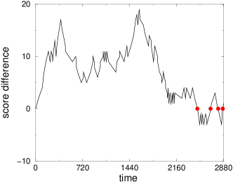
Figure 1: Evolution of the score difference in a typical NBA game: the Denver Nuggets vs. the Chicago Bulls on 26 November 2010. Dots indicate the four lead changes in the game. The Nuggets led for 2601 out of 2880 total seconds and won the game by a score of 98–97.

Scoring in professional basketball has several additional important features Gabel and Redner (2012); Merritt and Clauset (2014):

1. Nearly constant scoring rate throughout the game, except for small reductions at the start of the game and the second half, and a substantial enhancement in the last 2.5 minutes.

2. Essentially no temporal correlations between successive scoring events.

3. Intrinsically different team strengths. This feature may be modeled by a bias in the underlying random walk that describes scoring.

4. Scoring antipersistence. Since the team that scores cedes ball possession, the probability that this team again scores next occurs with probability $p<\frac{1}{2}$.

5. Linear restoring bias. On average, the losing team scores at a slightly higher rate than the winning team, with the rate disparity proportional to the score difference.

A major factor for the scoring rate is the 24-second “shot clock,” in which a team must either attempt a shot that hits the rim of the basket within 24 seconds of gaining ball possession or lose its possession. The average time interval between scoring events is $\Delta t=2880/93.6=30.8$ seconds, consistent with the 24-second shot clock. In a random walk picture of scoring, the average number of scoring events in a game, $N\!=\!93.6$, together with $s\!=\!2.07$ points for an average event, would lead to an rms displacement of $x_{\rm rms}=\sqrt{Ns^{2}}$. However, this estimate does not account for the antipersistence of basketball scoring. Because a team that scores immediately cedes ball possession, the probability that this same team scores next occurs with probability $p\approx 0.36$. This antipersistence reduces the diffusion coefficient of a random walk by a factor $p/(1-p)\approx 0.562$ Gabel and Redner (2012); García-Pelayo (2007). Using this, we infer that the rms score difference in an average basketball game should be $\Delta S_{\rm rms}\approx\sqrt{pNs^{2}/(1-p)}\approx 15.01$ points. Given the crudeness of this estimate, the agreement with the empirical value of 13.15 points is satisfying.

A natural question is whether this final score difference is determined by random-walk fluctuations or by disparities in team strengths. As we now show, for a typical game, these two effects have comparable influence. The relative importance of fluctuations to systematics in a stochastic process is quantified by the Péclet number $\mathcal{P}\!e\!\equiv\!vL/2D$ Probstein (1994), where $v$ is the bias velocity, $L=vT$ is a characteristic final score difference, and $D$ is the diffusion coefficient. Let us now estimate the Péclet number for NBA basketball. Using $\Delta S_{\rm rms}=13.15$ points, we infer a bias velocity $v=13.15/2880\approx 0.00457$ points/sec under the assumption that this score difference is driven only by the differing strengths of the two competing teams. We also estimate the diffusion coefficient of basketball as $D=\frac{p}{1-p}(s^{2}/2\Delta t)\approx 0.0391$ (points)²/sec. With these values, the Péclet number of basketball is

$$\mathcal{P}\!e=\frac{vL}{2D}\approx 0.77\enspace.$$ (2)

Since the Péclet number is of the order of 1, systematic effects do not predominate, which accords with common experience—a team with a weak win/loss record on a good day can beat a team with a strong record on a bad day. Consequently, our presentation on scoring statistics is mostly based on the assumption of equal-strength teams. However, we also discuss the case of unequal team strengths for logical completeness.

As we will present below, the statistical properties of lead changes and lead magnitudes, and the probability that a lead is “safe,” i.e., will not be erased before the game is over, are well described by an unbiased random-walk model. The agreement between the model predictions and data is closest for basketball. For the other professional sports, some discrepancies with the random-walk model arise that may help identify alternative mechanisms for scoring dynamics.

II Number of Lead Changes and Fraction of Time Leading

Two simple characterizations of leads are: (i) the average number of lead changes $\mathcal{N}$ in a game, and (ii) the fraction of game time that a randomly selected team holds the lead. We define a lead change as an event where the score difference returns to zero (i.e., a tie score), but do not count the initial score of 0–0 as lead change. We estimate the number of lead changes by modeling the evolution of the score difference as an unbiased random walk.

Using $N=93.6$ scoring events per game, together with the well-known probability that an $N$-step random walk is at the origin, the random-walk model predicts $\sqrt{2N/\pi}\approx 8$ for a typical number of lead changes. Because of the antipersistence of basketball scoring, the above is an underestimate. More properly, we must account for the reduction of the diffusion coefficient of basketball by a factor of $p/(1-p)\approx 0.562$ compared to an uncorrelated random walk. This change increases the number of lead changes by a factor $1/\sqrt{0.562}\approx 1.33$, leading to roughly 10.2 lead changes. This crude estimate is close to the observed 9.4 lead changes in NBA games (Table 1).

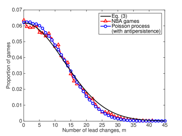
Figure 2: Distribution of the average number of lead changes per game in professional basketball.

For the distribution of the number of lead changes, we make use of the well-known result that the probability $G(m,N)$ that a discrete $N$-step random walk makes $m$ returns to the origin asymptotically has the Gaussian form $G(m,N)\sim e^{-m^{2}/2N}$ Weiss and Rubin (1983); Weiss (1984); Redner (2001). However, the antipersistence of basketball scoring leads to $N$ being replaced by $N\frac{1-p}{p}$, so that the probability of making $m$ returns to the origin is given by

$$G(m,N)\simeq\sqrt{\frac{2p}{\pi N(1-p)}}\,\,e^{-m^{2}p/[2N(1-p)]}\enspace.$$ (3)

Thus $G(m,N)$ is broadened compared to the uncorrelated random-walk prediction because lead changes now occur more frequently. The comparison between the empirical NBA data for $G(m,N)$ and a simulation in which scoring events occur by an antipersistent Poisson process (with average scoring rate of one event every 30.8 seconds), and Eq. (3) is given in Fig. 2.

For completeness, we now analyze the statistics of lead changes for unequally matched teams. Clearly, a bias in the underlying random walk for scoring events decreases the number of lead changes. We use a suitably adapted continuum approach to estimate the number of lead changes in a simple way. We start with the probability that biased diffusion lies in a small range $\Delta x$ about $x=0$:

$$\frac{\Delta x}{\sqrt{4\pi Dt}}\,\,e^{-v^{2}t/4D}\enspace.$$

Thus the local time that this process spends within $\Delta x$ about the origin up to time $t$ is

$$\mathcal{T}(t) =\Delta x\int_{0}^{t}\frac{dt}{\sqrt{4\pi Dt}}\,\,e^{-v^{2}t/4D}$$

$$=\frac{\Delta x}{v}\,\,\mathrm{erf}\big{(}\sqrt{{v^{2}t}/{4D}}\big{)}\enspace,$$ (4)

where we used $w=\sqrt{v^{2}t/4D}$ to transform the first line into the standard form for the error function. To convert this local time to number of events, $\mathcal{N}(t)$, that the walk remains within $\Delta x$, we divide by the typical time $\Delta t$ for a single scoring event. Using this, as well as the asymptotics of the error function, we obtain the limiting behaviors:

$$\mathcal{N}(t)=\frac{\mathcal{T}(t)}{\Delta t}\sim\begin{cases}\sqrt{{v_{0}^{2}t}/{\pi D}}&\qquad{v^{2}t}/{4D}\ll 1\\ {v_{0}}/{v}&\qquad{v^{2}t}/{4D}\gg 1\enspace,\end{cases}$$ (5)

with $v_{0}={\Delta x}/{\Delta t}$ and $\Delta x$ the average value of a single score (2.07 points). Notice that $v^{2}T/4D=\mathcal{P}\!e/2$, which, from Eq. (2), is roughly 0.38. Thus, for the NBA, the first line of Eq. (5) is the realistic case. This accords with what we have already seen in Fig. 2, where the distribution in the number of lead changes is accurately accounted for by an unbiased, but antipersistent random walk.

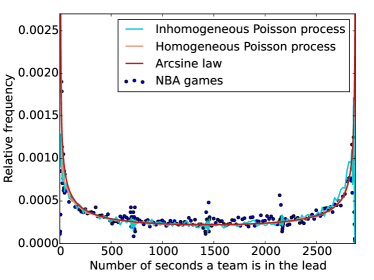
Figure 3: The distribution of the time that a given team holds the lead, $\mathcal{O}(t)$.

Another basic characteristic of lead changes is the amount of game time that one team spends in the lead, $\mathcal{O}(t)$, a quantity that has been previously studied for basketball Gabel and Redner (2012). Strikingly, the probability distribution for this quantity is bimodal, in which $\mathcal{O}(t)$ sharply increases as the time approaches either 0 or $T$, and has a minimum when the time is close to ${T}/{2}$. If the scoring dynamics is described by an unbiased random walk, then the probability that one team leads for a time $t$ in a game of length $T$ is given by the first arcsine law of Eq. (1) Feller (1968); Redner (2001). Figure 3 compares this theoretical result with basketball data. Also shown are two types of synthetically generated data. For the “homogeneous Poisson process”, we use the game-averaged scoring rate to generate synthetic basketball-game time series of scoring events. For the “inhomogeneous Poisson process”, we use the empirical instantaneous scoring rate for each second of the game to generate the synthetic data (Fig. 5). As we will justify in the next section, we do not incorporate the antipersistence of basketball scoring in these Poisson processes because this additional feature minimally influences the distributions that follow the arcsine law ($\mathcal{O}$, $\mathcal{L}$ and $\mathcal{M}$). The empirically observed increased scoring rate at the end of each quarter Gabel and Redner (2012); Merritt and Clauset (2014), leads to anomalies in the data for $\mathcal{O}(t)$ that are accurately captured by the inhomogeneous Poisson process.

III Time of the Last Lead Change

We now determine when the last lead change occurs. For the discrete random walk, the probability that the last lead occurs after $N$ steps can be solved by exploiting the reflection principle Feller (1968). Here we solve for the corresponding distribution in continuum diffusion because this formulation is simpler and we can readily generalize to unequal-strength teams. While the distribution of times for the last lead change is well known Lévy (1939, 1948), our derivation is intuitive and elementary.

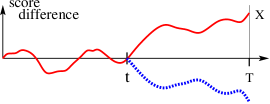
Figure 4: Schematic score evolution in a game of time $T$. The subsequent trajectory after the last lead change must always be positive (solid) or always negative (dashed).

For the last lead change to occur at time $t$, the score difference, which started at zero at $t\!=\!0$, must again equal zero at time $t$ (Fig. 4). For equal-strength teams, the probability for this event is simply the Gaussian probability distribution of diffusion evaluated at $x\!=\!0$:

$$P(0,t)=\frac{1}{\sqrt{4\pi Dt}}\enspace.$$ (6)

To guarantee that it is the last lead change that occurs at time $t$, the subsequent evolution of the score difference, cannot cross the origin between times $t$ and $T$ (Fig. 4). To enforce this constraint, the remaining trajectory between $t$ and $T$ must therefore be a time-reversed first-passage path from an arbitrary final point $(X,T)$ to $(0,t)$. The probability for this event is the first-passage probability Redner (2001)

$$F(X,T\!-\!t)=\frac{X}{\sqrt{4\pi D(T\!-\!t)^{3}}}\,\,e^{-X^{2}/[4D(T-t)]}\enspace.$$ (7)

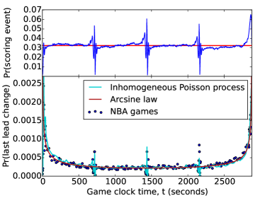
Figure 5: (upper) Empirical probability that a scoring event occurs at time $t$, with the game-average scoring rate shown as a horizontal line. The data is aggregated in bins of 10 seconds each; the same binning is used in Fig. 14. (lower) Distribution of times $\mathcal{L}(t)$ for the last lead change.

With these two factors, the probability that the last lead change occurs at time $t$ is given by

$$\mathcal{L}(t) =2\!\int_{0}^{\infty}\!dX\,P(0,t)\,F(X,T\!-\!t)$$

$$=2\!\int_{0}^{\infty}\!\!\frac{dX}{\sqrt{4\pi Dt}}\frac{X}{\sqrt{4\pi D(T\!-\!t)^{3}}}\,\,e^{-X^{2}/[4D(T\!-\!t)]}\,.$$ (8)

The leading factor 2 appears because the subsequent trajectory after time $t$ can equally likely be always positive or always negative. The integration is elementary and the result is the classic second arcsine law Lévy (1939, 1948) given in Eq. (1). The salient feature of this distribution is that the last lead change in a game between evenly matched teams is most likely to occur either near the start or the end of a game, while a lead change in the middle of a game is less likely.

As done previously for the distribution of time $\mathcal{O}(t)$ that one team is leading, we again generate a synthetic time series that is based on a homogeneous and an inhomogeneous Poisson process for individual scoring events without antipersistence. From these synthetic histories, we extract the time for the last lead and its distribution. The synthetic inhomogeneous Poisson process data accounts for the end-of-quarter anomalies in the empirical data with remarkable accuracy (Fig. 5).

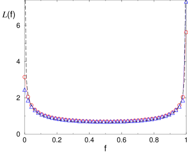
Figure 6: The distribution of time for the last lead change, $\mathcal{L}(f)$, as a function of the fraction of steps $f$ for a 94-step random walk with persistence parameter $p\!=\!0.36$ as in the NBA ($\circ$) and $p\!=\!0.25$ corresponding to stronger persistence ($\bigtriangleup$). The smooth curve is the arcsine law for $p\!=\!0.5$ (no antipersistence).

Let us now investigate the role of scoring antipersistence on the distribution $\mathcal{L}(t)$. While the antipersistence substantially affects the number of lead changes and its distribution, antipersistence has a barely perceptible effect on $\mathcal{L}(t)$. Figure 6 shows the probability $\mathcal{L}(f)$ that the last lead change occurs when a fraction $f$ of the steps in an $N$-step antipersistent random walk have occurred, with $N\!=\!94$, the closest even integer to the observed value $N\!=\!93.56$ of NBA basketball. For the empirical persistence parameter of basketball, $p=0.36$, there is little difference between $\mathcal{L}(f)$ as given by the arcsine law and that of the data, except at the first two and last two steps of the walk. Similar behavior arises for the more extreme case of persistence parameter $p=0.25$. Thus basketball scoring antipersistence plays little role in determining the time at which the last lead change occurs.

We may also determine the role of a constant bias on $\mathcal{L}(t)$, following the same approach as that used for unbiased diffusion. Now the analogues of Eqs. (6) and (7) are Redner (2001),

$$\begin{split}P(0,v,t)&=\frac{1}{\sqrt{4\pi Dt}}\,\,e^{-v^{2}t/4D}\\ F(X,v,t)&=\frac{X}{\sqrt{4\pi Dt^{3}}}\,\,e^{-(X+vt)^{2}/4Dt}\enspace.\end{split}$$ (9)

Similarly, the analogue of Eq. (III) is

$$\mathcal{L}(t)=\int_{0}^{\infty}\!\!\!dX\,P(0,t)\,\big{[}F(X,v,T\!-\!t)\!+\!F(X,-v,T\!-\!t)\big{]}\,.$$ (10)

In Eq. (9) we must separately consider the situations where the trajectory for times beyond $t$ is strictly positive (stronger team ultimately wins) or strictly negative (weaker team wins). In the former case, the time-reversed first-passage path from $(X,T)$ to $(0,t)$ is accomplished in the presence of a positive bias $+v$, while in the latter case, this time-reversed first passage occurs in the presence of a negative bias $-v$.

Explicitly, Eq. (10) is

$$\mathcal{L}(t) =\frac{e^{-v^{2}t/4D}}{\sqrt{4\pi Dt}}\int_{0}^{\infty}\!\!\!dX\frac{X}{\sqrt{4\pi D(T\!-\!t)^{3}}}\,\,$$

$$\hskip 50.58878pt\times\left\{e^{-(X+a)^{2}/b}+e^{-(X-a)^{2}/b}\right\}\,,$$ (11)

with $a=v(T-t)$ and $b=4D(T-t)$. Straightforward calculation gives

$$\mathcal{L}(t) =\frac{e^{-v^{2}t/4D}}{\pi\sqrt{t(T\!-\!t)}}\left\{\sqrt{\frac{\pi v^{2}(T\!-\!t)}{4D}}\,\,\mathrm{erf}\bigg{(}\sqrt{\frac{v^{2}(T\!-\!t)}{4D}}\,\bigg{)}\right.$$

$$\hskip 93.95122pt\left.+e^{-v^{2}(T\!-\!t)/4D}\right\}\,.$$ (12)

This form for $\mathcal{L}(t)$ is again bimodal (Fig. 7), as in the arcsine law, but the last lead change is now more likely to occur near the beginning of the game. This asymmetry arises because once a lead is established, which is probable because of the bias, the weaker team is unlikely to achieve another tie score.

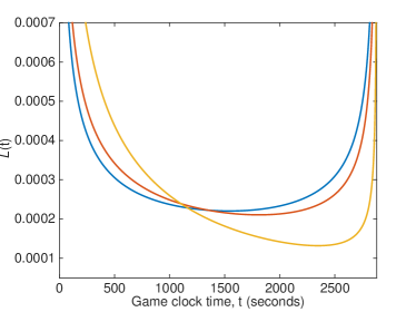
Figure 7: The distribution $\mathcal{L}(t)$ for non-zero bias (Eq. (III)). The diffusion coefficient is the empirical value $D=0.0391$, and bias values are: $v=0.002$, $v=0.004$, and $v=0.008$ (increasingly asymmetric curves). The central value of $v$ roughly corresponds to average NBA game-scoring bias if diffusion is neglected.

More germane to basketball, we should average $\mathcal{L}(t)$ over the distribution of biases in all NBA games. For this averaging, we use the observation that many statistical features of basketball are accurately captured by employing a Gaussian distribution of team strengths with mean value 1 (since the absolute strength is immaterial), and standard deviation of approximately 0.09  Gabel and Redner (2012). This parameter value was inferred by using the Bradley-Terry competition model Bradley and Terry (1952), in which teams of strengths $S_{1}$ and $S_{2}$ have scoring rates $S_{1}/(S_{1}+S_{2})$ and $S_{2}/(S_{1}+S_{2})$, respectively, to generate synthetic basketball scoring time series. The standard deviation 0.09 provided the best match between statistical properties that were computed from the synthetic time series and the empirical game data Gabel and Redner (2012). From the distribution of team strengths, we then infer a distribution of biases for each game and finally average over this bias distribution to obtain the bias-averaged form of $\mathcal{L}(t)$. The skewness of the resulting distribution is minor and it closely matches the bias-free form of $\mathcal{L}(t)$ given in Fig. 5. Thus, the bias of individual games appears to again play a negligible role in statistical properties of scoring, such as the distribution of times for the last lead change.

IV Time of the Maximal Lead

We now ask when the maximal lead occurs in a game Majumdar et al. (2008). If the score difference evolves by unbiased diffusion, then the standard deviation of the score difference grows as $\sqrt{t}$. Naively, this behavior might suggest that the maximal lead occurs near the end of a game. In fact, however, the probability $\mathcal{M}(t)$ that the maximal lead occurs at time $t$ also obeys the arcsine law Eq. (1). Moreover, the arcsine laws for the last lead time and for the maximal lead time are equivalent Lévy (1939, 1948); Mörters and Peres (2010), so that the largest lead in a game between two equally-matched teams is most likely to occur either near the start or near the end of a game.

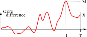
Figure 8: The maximal lead (which could be positive or negative) occurs at time $t$.

For completeness, we sketch a derivation for the distribution $\mathcal{M}(t)$ by following the same approach used to find $\mathcal{L}(t)$. Referring to Fig. 8, suppose that the maximal lead $M$ occurs at time $t$. For $M$ to be a maximum, the initial trajectory from $(0,0)$ to $(M,t)$ must be a first-passage path, so that $M$ is never exceeded prior to time $t$. Similarly, the trajectory from $(M,t)$ to the final state $(X,T)$ must also be a time-reversed first-passage path from $(X,T)$ to $(M,t)$, but with $X<M$, so that $M$ is never exceeded for all times between $t$ and $T$.

Figure 9: Distribution of times $\mathcal{M}(t)$ for the maximal lead.

Based on this picture, we may write $\mathcal{M}(t)$ as

$$\mathcal{M}(t) =A\int_{0}^{\infty}\!dM\,F(M,t)\int_{-\infty}^{M}\!dX\,F(X\!-\!M,T\!-\!t)$$

$$=A\int_{0}^{\infty}\!dM\frac{M}{\sqrt{4\pi Dt^{3}}}\,\,e^{-M^{2}/4Dt}$$

$$\hskip 18.06749pt\times\int_{-\infty}^{M}\!dX\frac{(M\!-\!X)}{\sqrt{4\pi D(T\!-\!t)^{3}}}\,\,e^{-(M\!-\!X)^{2}/4D(T\!-\!t)}\,.$$ (13)

The constant $A$ is determined by the normalization condition $\int_{0}^{T}\mathcal{M}(t)dt\!=\!1$. Performing the above two elementary integrations yields again the arcsine law of Eq. (1). Figure 9 compares the arcsine law prediction with empirical data from the NBA.

V Probability that a Lead is Safe

Finally, we turn to the question of how safe is a lead of a given size at any point in a game (Fig. 10), i.e., the probability that the team leading at time $t$ will ultimately win the game. The probability that a lead of size $L$ is safe when a time $\tau$ remains in the game is, in general,

$$Q(L,\tau) =1-\int_{0}^{\tau}\!\!F(L,t)\,dt\,.$$ (14)

where $F(L,t)$ again is the first-passage probability [Eqs. (7) and (9)] for a diffusing particle, which starts at $L$, to first reach the origin at time $t$. Thus the right-hand side is the probability that the lead has not disappeared up to time $\tau$.

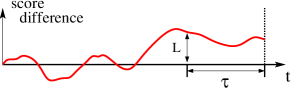
Figure 10: One team leads by $L$ points when a time $\tau$ is left in the game.

First consider evenly-matched teams, i.e., bias velocity $v=0$. We substitute $u=L/\sqrt{4Dt}$ in Eq. (14) to obtain

$$Q(L,\tau)=1-\frac{2}{\sqrt{\pi}}\int_{z}^{\infty}e^{-u^{2}}\,du=\mathrm{erf}(z)\enspace.$$ (15)

Here $z\equiv L/\sqrt{4D\tau}$ is the dimensionless lead size. When $z\!\ll\!1$, either the lead is sufficiently small or sufficient game time remains that a lead of scaled magnitude $z$ is likely to be erased before the game ends. The opposite limit of $z\!\gg\!1$ corresponds to either a sufficiently large lead or so little time remaining that this lead likely persists until the end of the game. We illustrate Eq. (15) with a simple numerical example from basketball. From this equation, a lead of scaled size $z\approx 1.163$ is 90% safe. Thus a lead of 10 points is 90% safe when 7.87 minutes remain in a game, while an 18-point lead at the end of the first half is also 90% safe .

Figure 11: Probability that a lead is safe versus the dimensionless lead size $z=L/\sqrt{4D\tau}$ for NBA games, showing the prediction from Eq. (15), the empirical data, and the mean prediction for Bill James’ well-known “safe lead” heuristic.

Figure 11 compares the prediction of Eq. (15) and the empirical basketball data. We also show the prediction of the heuristic developed by basketball analyst and historian Bill James James (2008). This rule is mathematically given by: $Q(L,\tau)=\min\left\{1,\frac{1}{\tau}(L\!-\!3\!+\!\delta/2)^{2}\right\}$, where $\delta=+1$ if the leading team has ball possession and $\delta=-1$ otherwise. The figure shows the predicted probability for $\delta=\{-1,0,+1\}$ (solid curve for central value, dashed otherwise) applied to all of the empirically observed $(L,\tau)$ pairs, because ball possession is not recorded in our data. Compared to the random walk model, the heuristic is quite conservative (assigning large safe lead probabilities only for dimensionless leads $z>2$) and has the wrong qualitative dependence on $z$. In contrast, the random walk model gives a maximal overestimate of 6.2% for the safe lead probability over all $z$, and has the same qualitative $z$ dependence as the empirical data.

For completeness, we extend the derivation for the safe lead probability to unequal-strength teams by including the effect of a bias velocity $v$ in Eq. (14):

$$Q(L,\tau) =1-\int_{0}^{\tau}\!\!\frac{L}{\sqrt{4\pi Dt^{3}}}\,\,e^{-(L+vt)^{2}/4Dt}\,dt$$

$$=1-e^{-vL/2D}\!\int_{0}^{\tau}\!\!\frac{L}{\sqrt{4\pi Dt^{3}}}\,\,e^{-L^{2}/4Dt-v^{2}t/4D}\,dt\,,$$ (16)

where the integrand in the first line is the first-passage probability for non-zero bias. Substituting $u=L/\sqrt{4Dt}$ and using again the Péclet number $\mathcal{P}\!e=vL/2D$, the result is

$$Q(L,\tau) =1-\frac{2}{\sqrt{\pi}}\,\,e^{-\mathcal{P}\!e}\int_{0}^{z}e^{-u^{2}-\mathcal{P}\!e^{2}/4u^{2}}\,du$$

$$=1-\tfrac{1}{2}\!\left[e^{-2\mathcal{P}\!e}\mathrm{erfc}\Big{(}z\!-\!\frac{\mathcal{P}\!e}{2z}\Big{)}\!+\!\mathrm{erfc}\Big{(}z\!+\!\frac{\mathcal{P}\!e}{2z}\Big{)}\right]\enspace.$$ (17)

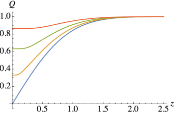
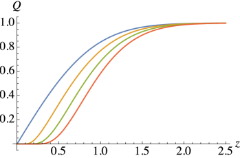
Figure 12: Probability that a lead is safe versus $z=L/\sqrt{4D\tau}$ for: (a) the stronger team is leading for $\mathcal{P}\!e=\frac{1}{5}$, $\frac{1}{2}$ and 1, and (b) the weaker team is leading for $\mathcal{P}\!e=-\frac{2}{5}$, $-\frac{4}{5}$ and $-\frac{6}{5}$. The case $\mathcal{P}\!e=0$ is also shown for comparison.

When the stronger team is leading ($\mathcal{P}\!e>0$), essentially any lead is safe for $\mathcal{P}\!e\gtrsim 1$, while for $\mathcal{P}\!e<1$, the safety of a lead depends more sensitively on $z$ (Fig. 12(a)). Conversely, if the weaker team happens to be leading ($\mathcal{P}\!e<0$), then the lead has to be substantial or the time remaining quite short for the lead to be safe (Fig. 12(b)). In this regime, the asymptotics of the error function gives $Q(L,\tau)\sim e^{-\mathcal{P}\!e^{2}/4z^{2}}$ for $z<|\mathcal{P}\!e|/2$, which is vanishingly small. For values of $z$ in this range, the lead is essentially never safe.

VI Lead changes in other sports

We now consider whether our predictions for lead change statistics in basketball extend to other sports, such as college American football (CFB), professional American football (NFL), and professional hockey (NHL) . These sports have the following commonalities with basketball Merritt and Clauset (2014):

1. Two teams compete for a fixed time $T$, in which points are scored by moving a ball or puck into a special zone in the field.

2. Each team accumulates points during the game and the team with the largest final score is the winner (with sport-specific tiebreaking rules).

3. A roughly constant scoring rate throughout the game, except for small deviations at the start and end of each scoring period.

4. Negligible temporal correlations between successive scoring events.

5. Intrinsically different team strengths.

6. Scoring antipersistence, except for hockey.

These similarities suggest that a random-walk model should also apply to lead change dynamics in these sports.

However, there are also points of departure, the most important of which is that the scoring rate in these sports is between 10–25 times smaller than in basketball. Because of this much lower overall scoring rate, the diminished rate at the start of games is much more apparent than in basketball (Fig. 14). This longer low-activity initial period and other non-random-walk mechanisms cause the distributions $\mathcal{L}(t)$ and $\mathcal{M}(t)$ to visibly deviate from the arcsine laws (Figs. 14 and 15). A particularly striking feature is that $\mathcal{L}(t)$ and $\mathcal{M}(t)$ approach zero for $t\to 0$. In contrast, because the initial reduced scoring rate occurs only for the first 30 seconds in NBA games, there is a realu, but barely discernible deviation of the data for $\mathcal{L}(t)$ from the arcsine law (Fig. 5).

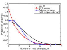
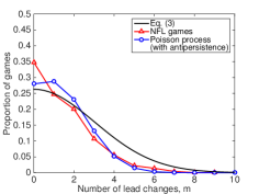
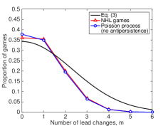
Figure 13: Distribution of the average number of lead changes per game, for CFB, NFL, and NHL, showing the simple prediction of Eq. (3), the empirical data, and the results of a simulation in which scoring events occur by a Poisson process with the game-specific scoring rate.

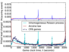
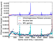
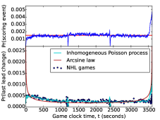
Figure 14: (upper) Empirical probability that a scoring event occurs at time $t$, with the game-average scoring rate shown as a horizontal line, for games of CFB, NFL, and NHL. (lower) Distribution of times $\mathcal{L}(t)$ for the last lead change.

Finally, the safe lead probability given in Eq. (15) qualitatively matches the empirical data for football and hockey (Fig. 16), with the hockey data being closest to the theory . For both basketball and hockey, the expression for the safe lead probability given in Eq. (15) is quantitatively accurate. For football, a prominent feature is that small leads are much more safe that what is predicted by our theory. This trend is particularly noticeable in the CFB. One possible explanation of this behavior is that in college football, there is a relatively wide disparity in team strengths, even in the most competitive college leagues. Thus a small lead size can be quite safe if the two teams happen to be significantly mismatched.

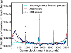
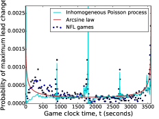
Figure 15: Distribution of times $\mathcal{M}(t)$ for the maximal lead, for games of CFB, NFL, and NHL.

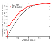
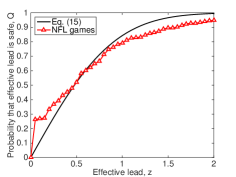
Figure 16: Probability that a lead is safe, for CFB, NFL, and NHL, versus the dimensionless lead $z=L/\sqrt{4D\tau}$. Each figure shows the prediction from Eq. (15) and the corresponding empirical pattern.

For American football and hockey, it would be useful to understand how the particular structure of these sports would modify a random walk model. For instance, in American football, the two most common point values for scoring plays are 7 (touchdown plus extra point) and 3 (field goal). The random-walk model averages these events, which will underestimate the likelihood that a few high-value events could eliminate what otherwise seems like a safe lead. Moreover, in football the ball is moved incrementally down the field through a series of plays. The team with ball possession has four attempts to move the ball a specific minimum distance (10 yards) or else lose possession; if it succeeds, that team retains possession and repeats this effort to further move the ball. As a result, the spatial location of the ball on the field likely plays an important role in determining both the probability of scoring and the value of this event (field goal versus touchdown). In hockey, players are frequently rotated on and off the ice so that a high intensity of play is maintained throughout the game. Thus the pattern of these substitutions— between potential all-star players and less skilled “grinders”—can change the relative strength of the two teams every few minutes.

VII Conclusions

A model based on random walks provides a remarkably good description for the dynamics of scoring in competitive team sports. From this starting point, we found that the celebrated arcsine law of Eq. (1) closely describes the distribution of times for: (i) one team is leading $\mathcal{O}(t)$ (first arcsine law), (ii) the last lead change in a game $\mathcal{L}(t)$ (second arcsine law), and (iii) when the maximal lead in the game occurs $\mathcal{M}(t)$ (third arcsine law). Strikingly, these arcsine distributions are bimodal, with peaks for extremal values of the underlying variable. Thus both the time of the last lead and the time of the maximal lead are most likely to occur at the start or the end of a game.

These predictions are in accord with the empirically observed scoring patterns within more than 40,000 games of professional basketball, American football (college or professional), and professional hockey. For basketball, in particular, the agreement between the data and the theory is quite close. All the sports also exhibit scoring anomalies at the end of each scoring period, which arise from a much higher scoring rate around these times (Figs. 5 and 14). For football and hockey, there is also a substantial initial time range of reduced scoring that is reflected in $\mathcal{L}(t)$ and $\mathcal{M}(t)$ both approaching zero as $t\to 0$. Football and hockey also exhibit other small but systematic deviations from the second and third arcsine laws that remain unexplained.

The implication for basketball, in particular, is that a typical game can be effectively viewed as repeated coin-tossings, with each toss subject to the features of antipersistence, an overall bias, and an effective restoring force that tends to shrink leads over time (which reduces the likelihood of a blowout). These features represent inconsequential departures from a pure random-walk model. Cynically, our results suggest that one should watch only the first few and last few minutes of a professional basketball game; the rest of the game is as predictable as watching repeated coin tossings. On the other hand, the high degree of unpredictability of events in the middle of a game may be precisely what makes these games so exciting for sports fans.

The random-walk model also quantitatively predicts the probability that a specified lead of size $L$ with $t$ seconds left in a game is “safe,” i.e., will not be reversed before the game ends. Our predictions are quantitatively accurate for basketball and hockey. For basketball, our approach significantly outperforms a popular heuristic for determining when a lead is safe. For football, our prediction is marginally less accurate, and we postulated a possible explanation for why this inaccuracy could arise in college football, where the discrepancy between the random-walk model and the data is the largest.

Traditional analyses of sports have primarily focused on the composition of teams and the individual skill levels of the players. Scoring events and game outcomes are generally interpreted as evidence of skill differences between opposing teams. The random walk view that we formalize and test here is not at odds with the more traditional skill-based view. Our perspective is that team competitions involve highly skilled and motivated players who employ well-conceived strategies. The overarching result of such keen competition is to largely negate systematic advantages so that all that remains is the residual stochastic element of the game. The appearance of the arcsine law, a celebrated result from the theory of random walks, in the time that one team leads, the time of the last lead change, and the time at which the maximal lead occurs, illustrates the power of the random-walk view of competition. Moreover, the random-walk model makes surprisingly accurate predictions of whether a current lead is effectively safe, i.e., will not be overturned before the game ends, a result that may be of practical interest to sports enthusiasts.

The general agreement between the random-walk model for lead-change dynamics across four different competitive team sports suggests that this paradigm has much to offer for the general issue of understanding human competitive dynamics. Moreover, the discrepancies between the empirical data and our predictions in sports other than basketball may help identify alternative mechanisms for scoring dynamics that do not involve random walks. Although our treatment focused on team-level statistics, another interesting direction for future work would be to focus on understanding how individual behaviors within such social competitions aggregate up to produce a system that behaves effectively like a simple random walk. Exploring these and other hypotheses, and developing more accurate models for scoring dynamics, are potential fruitful directions for further work.