Modeling water uptake by a root system growing in a fixed soil volume.

Abstract

The water uptake by roots of plants is examined for an ideal situation, with an approximation that resembles plants growing in pots, meaning that the total soil volume is fixed. We propose a coupled water uptake-root growth model. A one-dimensional model for water flux and water uptake by a root system growing uniformly distributed in the soil is presented, and the Van Genuchten model for the transport of water in soil is used. The governing equations are represented by a moving boundary model for which the root length, as a function of time, is prescribed. The solution of the model is obtained by front-fixing and finite element methods. Model predictions for water uptake by a same plant growing in loam, silt and clay soils are obtained and compared. A sensitivity analysis to determine relative effects on water uptake when system parameters are changed is also presented and shows that the model and numerical method proposed are more sensitive to the root growth rate than to the rest of the parameters. This sensitivity decreases along time, reaching its maximum at thirty days. A comparison of this model with a fixed boundary model with and without root growth is also made. The results show qualitative differences from the beginning of the simulations, and quantitative differences after ten days of simulations.

1 Introduction

In the development of a theory to describe plant water uptake, electrical analogues of the system have been used for analysis [1, 2, 3]. The analogues are based on the assumption that rooting patterns are uniform and constant in each soil layer. Steady flow is presumed in both the soil and the plant over the period of calculation. In this approach the plant water potentials are primarily the result of an imposed value of transpiration rate and its variations. Later papers [4, 5, 6] have presented detailed reviews on plant water uptake. In those papers the Richards equation is used, with a sink term. Another approach is to model the water movement and uptake over large areas, using individual plant [7], or global behavior [8]. A microscopical approach has also been proposed [9], where the total water uptake is calculated based on using a constant value for the entire rooting profile. In more recent papers [10, 11, 12] the root growth has been taken into account, still using a fixed domain. The root growth is inscribed on a domain that is not a function of time. Some other papers about nutrient uptake consider root growth and instantaneous coupling with the nutrient flux by using a variable domain approximation [13]. In this last model [13] a variable root length, and consequently, a variable available volume of soil to each root of a root system is considered using a moving boundary model. In this model the root system is uniformly distributed in the soil and the variation of available soil volume per unit of root length is modeled by a moving boundary. The approach presented here is based on that in [13] . In the proposed model plants growing in controlled conditions, as in a growth chamber, are assumed. A constant temperature and evapotranspiration rate is presumed. In this situation, the water potential at the root surface is determined by the soil water potential, and consequently determines water uptake by the growing root system. The proposed model considers an uniform root water uptake for all the root system. The goal of this paper is to present a simplified model of water uptake coupled with a growing root system and analyze the influence of system parameters on water uptake using typical values.

2 Model

Darcy’s law describes the flow of water on a porous unsaturated medium as

$$\vec{J}(\vec{r},t)=-K(\Psi(\vec{r},t))\vec{\nabla}\Psi(\vec{r},t)$$ (1)

with $\vec{J}[cm^{3}/cm^{2}s]$ the water flux per surface unit at position $\vec{r}[cm]$ at time $t[s]$, $K[cm/s]$ the soil water conductivity and $\Psi[cm]$ the soil water potential.

The corresponding continuity equation (mass conservation) is given by

$$-\nabla\cdot\vec{J}=\frac{\partial\theta}{\partial t},$$ (2)

with $\theta[cm^{3}/cm^{3}]$ the soil water content per unit of volume, with the approximation of only radial flux the transport equation results

$$\frac{\partial}{\partial t}\left[\Psi(r,t)\right]=-\frac{1}{rC(\Psi(r,t))}\frac{\partial}{\partial r}\left[rK(\Psi(r,t))\frac{\partial}{\partial r}\left[\Psi(r,t)\right]\right]$$ (3)

where $r$ is the cylindrical radial coordinate, and

$$C(\Psi(r,t))=\frac{d\theta}{d\Psi}(\Psi(r,t))$$ (4)

is the differential capacity of water $[cm^{-1}]$.

The soil water constitutive relations for $K$, $\theta$, and $C$, as functions of $\Psi$, are the ones proposed by Van Genuchten [14], and consist of the expressions given by:

$$K(\Psi) = K_{s}\frac{\left\{\left[1+\left(\frac{\Psi}{\Psi_{e}}\right)^{n}\right]^{m}-\left(\frac{\Psi}{\Psi_{e}}\right)^{n-1}\right\}^{2}}{\left[1+\left(\frac{\Psi}{\Psi_{e}}\right)^{n}\right]^{m(p+2)}},$$ (5)

$$\theta(\Psi) = \left[1+\left(\frac{\Psi}{\Psi_{e}}\right)^{n}\right]^{-m}(\theta_{s}-\theta_{R})+\theta_{R},$$ (6)

$$C(\Psi) = (\theta_{s}-\theta_{R})\frac{1-n}{\Psi_{e}}\left[1+\left(\frac{\Psi}{\Psi_{e}}\right)^{n}\right]^{-m-1}\left(\frac{\Psi}{\Psi_{e}}\right)^{n-1},$$ (7)

where $K_{s}[cm/s]$ is the saturated soil conductivity, $\theta_{s}[cm^{3}/cm^{3}]$ is the saturated soil water content, $\theta_{R}[cm^{3}/cm^{3}]$ is the residual water content, $\Psi_{e}[cm]$, $p[1]$ and $n[1]$ are experimental coefficients, and $m=1-1/n$.

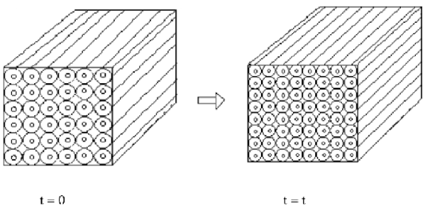
Figure 1: Homogeneous rooting in soil and its time evolution.

We presume that the water potential does not change with soil depth, the soil does not evaporate, and laboratory conditions, like light and temperature are maintained constant. The root density is homogeneous on the soil, the total volume is fixed (as in pots), therefore the soil volume per unit of root length is decreasing as in Figure 1. Based on these assumptions, and taking into account the root length density as a function of time $(t)$ the following moving boundary model in cylindrical coordinates [9, 13] is proposed

$$\frac{\partial}{\partial t}\left[\Psi(r,t)\right] = -\frac{1}{rC(\Psi(r,t))}\frac{\partial}{\partial r}\left[rK(\Psi(r,t))\frac{\partial}{\partial r}\left[\Psi(r,t)\right]\right]$$ (8)

$$\Psi(r,0) = \phi(r)$$ (9)

$$H\left(\Psi(R(t),t),t\right) = 2\pi R(t)K(\Psi(R(t),t))\frac{\partial\Psi}{\partial r}(R(t),t)$$ (10)

$$G\left(\Psi(s_{0},t)\right) = -2\pi s_{0}K(\Psi(s_{0},t))\frac{\partial\Psi}{\partial r}(s_{0},t)$$ (11)

$$R(t) = R_{0}\sqrt{\frac{l_{0}}{l(t)}}$$ (12)

with $s_{0}\leq r\leq R(t)$ and $0\leq t\leq T_{max}$, where $T_{max}$ is the maximum time for which the system has meaning $\left(R(T_{max})\geq s_{0}\right)$, $s_{0}$ is the root radius, $R_{0}$ is the initial half-distance among roots, $R(t)$ is the instantaneous half-distance among roots (a decreasing function as root density grows), $l_{0}$ is the initial root length, and $l(t)$ is the instantaneous root length. Equation (8) is the pressure head based Buckingham-Richards equation. The condition (9) is the initial water potential profile, with $\phi(r)$ a single valued function. The condition (10) represents the flux $(H)$ on the moving boundary $r=R(t)$, which will be considered null in this paper as an approximation to a soil isolated. The condition (11) is the boundary condition at the root soil interface $(r=s_{0})$ representing the root water uptake per unit of root length $\left(G(\Psi(s_{0},t))[cm^{3}/cm\ s]\right)$. For the water uptake function $\left(G(\Psi)\right)$ we use the function proposed by Feddes [4] which is given by:

$G(\Psi)=0$	if	$0>\Psi\geq\Psi_{1}$
$G(\Psi)=S_{max}$	if	$\Psi_{1}>\Psi\geq\Psi_{2}$
$G(\Psi)=S_{max}\frac{\Psi-\Psi 3}{\Psi_{2}-\Psi_{3}}$	if	$\Psi_{2}>\Psi\geq\Psi_{3}$
$G(\Psi)=0$	if	$\Psi_{3}>\Psi$

where $\Psi_{1}$, $\Psi_{2}$ and $\Psi_{3}$ are the anaerobiosis point, the limiting point, and the wilting point, respectively. $S_{max}\left[cm^{2}/s\right]$ is the maximum water uptake per unit of root length. A diagram of this function can be seen on Figure 2. The condition (12) is the time dependence of the moving boundary $(R(t))$ which is obtained presuming a fixed total volume including soil and roots, and a linear growth rate $(l(t)=l_{0}+V\ t)$ [13], where $V\left[cm/s\right]$ is the root length growth rate. Graphical evolution of this system with time can be seen in Figure 1. A schematic mathematical diagram of the problem is shown in Figure 3. Once the water potential $\Psi(s_{0},t)$ at the root surface is obtained, the water uptake is computed with a variable domain integration method given by [15]

$$U(t) = l_{0}\int_{0}^{t}G(\Psi(s_{0},\tau))d\tau$$ (13)

$$+\int_{0}^{t}\left(\int_{\tau}^{t}G(\Psi(s_{0},\tau))d\tau\right)\dot{l}(\tau)d\tau$$

where $U\left[cm^{3}\right]$ is the cumulative water uptake at time $t$. This last expression can be simplified to (see A)

$$U(t) = \int_{0}^{t}G(\Psi(s_{0},\tau))l(\tau)d\tau,$$ (14)

then the instantaneous water uptake can be defined as

$$U_{i}(t)=\dot{U}(t)=G(\Psi(s_{0},t))l(t).$$ (15)

The remaining soil water $\left(W\left[cm^{3}\right]\right)$ as a function of time can be calculated using

$$W(t)=2\pi\ l(t)\int_{s_{0}}^{R(t)}\theta\left(\Psi(r,t)\right)r\ dr,$$ (16)

if the root is not growing then $l(t)=l_{0}=constant$, and as a consequence $R(t)=R_{0}$, therefore the water remaining in the soil in this case is

$$W(t)=2\pi\ l_{0}\int_{s_{0}}^{R_{0}}\theta\left(\Psi(r,t)\right)r\ dr.$$ (17)

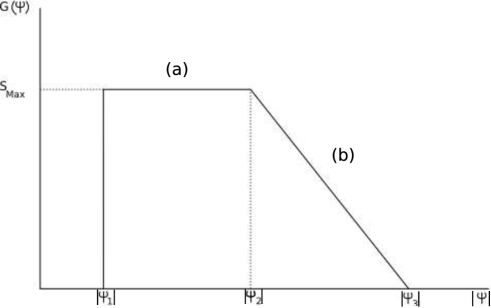
Figure 2: Root water uptake function as proposed by Feddes [4]. The zone (a) is the zone of maximum water uptake, while the zone (b) is the zone of linear water uptake.

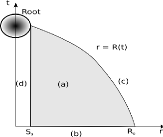
Figure 3: model of the domain of validity of the proposed model, the shaded zone (a) represents the zone where the equation (8) is valid. The line (b) is the initial value condition (9). In the curve (c) $r=R(t)$ the boundary condition (10) is used. In the line (d) the root water uptake condition (11) is used.

To solve the system (8)–(12) the domain is transformed to a dimensionless form by using the following expressions:

$$x = \frac{r-s_{0}}{R(t)-s_{0}},$$

$$\tau = \frac{t}{t_{0}},$$ (18)

$$\Phi(x,\tau) = \frac{\Psi(r,t)}{\Psi_{e}}=\frac{\Psi(x(R(t)-s_{0})+s_{0},\tau t_{0})}{\Psi_{e}},$$

or their inverses given by

$$r = s_{0}+(R(t)-s_{0})x$$

$$t = t_{0}\tau$$ (19)

$$\Psi(r,t) = \Psi_{e}\Phi\left(x,\tau\right)=\Psi_{e}\Phi\left(\frac{r-s_{0}}{R(t)-s_{0}},\frac{t}{t_{0}}\right).$$

and the following definitions

$$k(\Phi(x,\tau)) = \frac{K(\Psi(r,t))}{K_{s}}=\frac{\left\{\left[1+\Phi^{n}(x,\tau)\right]^{m}-\Phi^{n-1}(x,\tau)\right\}^{2}}{\left[1+\Phi^{n}(x,\tau)\right]^{m(p+2)}}$$ (20)

$$c(\Phi(x,\tau)) = \frac{C(\Psi(r,t))\Psi_{e}}{(\theta_{s}-\theta_{R})(1-n)}=\frac{\Phi^{n-1}(x,\tau)}{\left[1+\Phi^{n}(x,\tau)\right]^{m+1}}$$ (21)

$$v(\tau) = \frac{R(t)}{s_{0}}$$ (22)

$$w(\tau) = \frac{l(t)}{s_{0}}$$ (23)

$$g(\Phi(x,\tau)) = \frac{G(\Psi(r,t))}{S_{max}}$$ (24)

$$H(\Psi(r,t)) = 0,$$ (25)

$$c^{*}(\Phi(x,\tau),x,\tau) = \left((v(\tau)-1)x+1\right)c(\Phi(x,\tau))$$ (26)

$$k^{*}(\Phi(x,\tau),x,\tau) = \left((v(\tau)-1)x+1\right)k(\Phi(x,\tau))$$ (27)

$$\tilde{c}(\Phi(x,\tau),x,\tau) = -\frac{xv(\tau)w^{\prime}(\tau)}{2w(\tau)(v(\tau)-1)}c^{*}(\Phi(x,\tau),x,\tau)$$ (28)

$$v(\tau) = \frac{R_{0}}{s_{0}}\sqrt{\frac{l_{0}}{s_{0}w(\tau)}}$$ (29)

$$\gamma = \frac{t_{0}\Psi_{e}K_{s}}{(\theta_{s}-\theta_{R})(1-n)s_{0}^{2}}$$ (30)

$$\sigma = \frac{S_{max}}{2\pi K_{s}\Psi_{e}}$$ (31)

$$\tau_{max} = \frac{T_{max}}{t_{0}}$$ (32)

where $k(\Phi(x,\tau))$ and $c(\Phi(x,\tau))$ are the dimensionless forms of $K(\Psi(r,t))$ and $C(\Psi(r,t))$ respectively. The dimensionless number $\gamma$ takes into account soil properties and the geometrical proportions of the root, $t_{0}$ is chosen to make $\gamma=1$. The dimensionless number $\sigma$ takes into account one flux per unit of length, related to the water uptake, the term $K_{s}\Psi_{e}$ is a flux per unit of length when the soil is saturated and the gradient of the matric potential is equal to $\Psi_{e}/1cm$.

Taking into account (18) and the definitions (20)–(32), the system (8)–(12) is transformed in a dimensionless form in the domain $(0,1)\times(0,\tau_{max})$ given by:

$$c^{*}(\Phi(x,\tau),x,\tau)\frac{\partial}{\partial\tau}\left[\Phi(x,\tau)\right] = \tilde{c}(\Phi(x,\tau),x,\tau)\frac{\partial}{\partial x}\left[\Phi(x,\tau)\right]-$$

$$\frac{\partial}{\partial x}\left[\frac{\gamma k^{*}(\Phi(x,\tau),x,\tau)}{(v(\tau)-1)^{2}}\frac{\partial}{\partial x}\left[\Phi(x,\tau)\right]\right],$$

$$\Phi(x,0) = \varphi(x),$$ (34)

$$\frac{\partial\Phi}{\partial x}(1,\tau) = 0,$$ (35)

$$\sigma\ g(\Phi(0,\tau)) = -\frac{1}{v(\tau)-1}k^{*}(\Phi(0,\tau),0,\tau)\frac{\partial\Phi}{\partial x}(0,\tau),$$ (36)

where $\varphi(x)=\phi(s_{0}+(R_{0}-s_{0})x)/\Psi_{e}$, is the dimensionless initial profile. This transformation maps the spatial domain variable in time to a fixed domain in time, and adds a term on the right side of the transformed transport equation (2) which contains the variation of the moving boundary. In order to solve the model (2–36) the non-linear finite element method [16] is applied and the resulting model is solved by using the software FlexPDE [17] with an adaptive mesh of around 400 nodes.

3 Results

All simulations were performed by a same hypothetical plant in three types of soils (loam, silt and clay) for the same soil-root volume $(4000cm^{3})$ with the same total water content $(\theta_{i}=0.30)$. This initial condition is fixed using the ”field capacity” concept given by Ritchie [18]. Hydraulic soil data selected were those for loam, silt, and clay based on [9]. The soil parameters used are shown in Table 1. For the plant parameters different sources were used. The values of $\Psi_{2}$ and $\Psi_{3}$ were taken from [19], the value of $\Psi_{1}$ was chosen to assure that wateruptake was possible at the beginning of the simulation. $s_{0}$ and $V$ are typical values from the literature [20], and $l_{0}$ was chosen to be $1$ cm to simulate a plant at the start of growth. The plant and soil volume parameters are listed in Table 2. Table 3 shows parameters of soil and plant properties and the initial “available water”$(U_{0})$. This last parameter is approximated as

$$U_{0}=[\theta_{i}-\theta(\Psi_{3})]\times 4000cm^{3},$$ (37)

and represents how much water can be extracted from the soil before it reaches an uniform water potential at the wilting point. Beyond this point the root cannot extract more water.

Soil	$\theta_{s}$	$\theta_{R}$	$K_{s}$ (cm/s)	$\Psi_{e}$ (cm)	$n$	$p$
Loam	$0.43$	$0.078$	$2.89\times 10^{-4}$	$-27.78$	$1.56$	$0.5$
Silt	$0.46$	$0.034$	$7.00\times 10^{-5}$	$-62.5$	$1.37$	$0.5$
Clay	$0.38$	$0.068$	$5.80\times 10^{-6}$	$-125$	$1.09$	$0.5$

Table 1: Soil hydraulic properties

Parameter	Value
$l_{0}$	1	cm
$R_{0}$	35.7	cm
$V$	$1*10^{-4}$	cm/s
$s_{0}$	0.05	cm
$S_{max}$	$2*10^{-6}$	cm2/s
$\Psi_{1}$	-1	cm
$\Psi_{2}$	-750	cm
$\Psi_{3}$	-17500	cm

Table 2: Values for the plant and soil volume parameters

Soil	$\Psi(r,0)$ (cm)	$t_{0}$ (s)	$U_{0}$ (cm3)
Loam	$-51.4$	$0.0614$	$850$
Silt	$-194$	$0.0901$	$852$
Clay	$-3280$	$0.0968$	$128$

Table 3: Simulation parameters depending on soil and plant properties

Figures 4, 5, and 6 show the soil water potential profiles at different times, with an initial moisture condition equivalent $(\theta=0.30)$, for the loam, silt and clay soil, respectively. The curves reveal that a high water potential gradient is developed in a very small time period for the clay soil, while for the loam and silt soil the development of the water potential gradient is more gradual. For loam and silt soil the root dries the soil near the root surface on the first 30 days. After that period these soils show a water potential on the root surface close to the wilting point. The root starts to retrieve water near the moving boundary $R(t)$. This is shown by an increase of the modulus of the water potential (decrease of his value) at $x=1$ for the dimensionless domain, or $r=R(t)$ for the physical domain. The clay soil shows a similar behavior but the time period at which the potential near root zone reaches potentials close to the wilting point is 10 days.

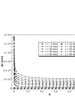
Figure 4: Water potential profiles at the scaled domain for the loam soil.

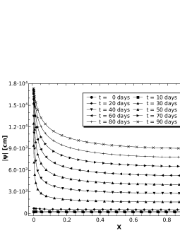
Figure 5: Water potential profiles at the scaled domain for the silt soil.

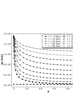
Figure 6: Water potential profiles at the scaled domain for the clay soil.

Figure 7 shows the relative water uptake $(G(\Psi(s_{0},t))/S_{max})$ per unit of root length as a function of time for the three types of soil, at different root growth rate. At the initial time the water uptake for loam and silt soil develops at the zone of maximum uptake (zone (a) in Figure 2), while clay soil does the same for the linear uptake zone (zone (b) in Figure 2). The figure shows that the water uptake does not vary much for the first 20 days as a function of $V$ for loam soil, after that period loam soil enters on the linear regime at different times depending on the value of $V$. After 40 days the gap among the curves on the log scale remains almost constant and all the curves are in the linear uptake regime. This means that the instantaneous root water uptake curves have a multiplicative constant among them. Silt soil has a very similar behavior to loam soil but the linear regime occurs at shorter times. For clay soil the period of similar water uptake is 10 days and after that period the curves begin a gradual separation that continues until the end of the simulation. Clay soil also shows a very sharp initial decrease on the curve (one order of magnitude), this is due to the linear regime and a large decrease of $\Psi(s_{0},t)$ at the beginning of the simulation.

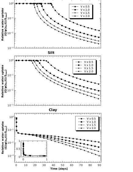
Figure 7: Relative water uptake per unit of root length time evolution for the different soils. The curves refer to changes in root growth speed $(V)$. The square is a zoom on the first day of simulation for the clay soil.

To compare the above simulations with those for a constant root length density in a fixed domain model a simulation with $V=0$ $(R(t)=R_{0})$ was made. For the comparison to be useful the root length was taken to be the average root length $(l_{0}=\bar{l}=389.8cm)$. Using this value the domain is fixed and the moving boundary model then becomes the model proposed by Personne [9]. The influxes on the root surface estimated by the fixed boundary model are then integrated using (14) with the fixed root length, to compute the cumulative uptake. This model will be referred to as Fixed Boundary Fixed Length (FBFL). Similar to published results on nutrient uptake (e.g. Claasen and Barber [21], Cushman [22]) the influxes obtained with the fixed boundary model can be integrated using equation (14) with a variable root length, to compute the cumulative uptake. This model will be referred to as Fixed Boundary Variable Length (FBVL). Figure 8 shows the instantaneous root system water uptake against time (i.e. $G(\Psi(s_{0},t))\times l(t)$), for the three models. The time at which the instantaneous water uptake is maximum is called the Maximum Uptake time (MUT). The MUT is only present when the roots are growing. The straight line in the beginning is caused by the assumption of linear root length growth and the constant water uptake $(G(\Psi)=S_{max})$, on the models with root growth. In contrast when the root is taking up water in the water stressed (linear zone) of the water uptake function the instantaneous water uptake as a function of time is non linear, in all models. We also observe that in the clay soil for the models with root growth the water uptake initially decreases given the large decrease in soil water potential at the root surface. This variation is shown in the inset, the later increase in water uptake is due to the root growth. The models with growing roots have a similar course in time, but the differences between the MUT-values are consistently showing that the MUT in the FBVL occurs earlier after the start of root growth. The instantaneous water uptake of the FBFL model and the FBVL models differs only by the multiplicative factor $l(t)/\bar{l}$.

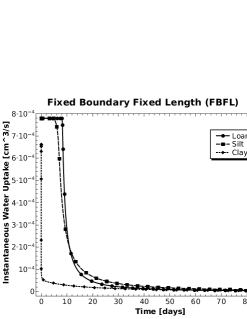
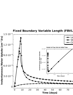
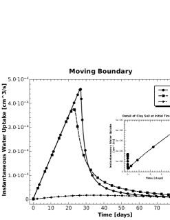
Figure 8: Instantaneous water uptake time evolution for the three models to be compared, from top to bottom fixed boundary without root growth, fixed boundary with root growth and moving boundary by the root growth.

Figure 9 shows the cumulative water uptake as a function of time for the three models. The cumulative water uptake at 90 days $(U(90))$ is close to the amount of water initially available $(U_{0})$ for the FBFL and the moving boundary models (see Table 3). For the FBVL model the cumulative water uptake is lower than that predicted by the other. This difference is due to the smaller value of the MUT. After 90 days $20\%$ of the initially available water in the clay soil is remaining, whereas for the silt and loam soil it is in the order of $10\%$. The clay soil does not trend to a constant value due to the less water uptake. It is expected that over a longer period the moisture content in the clay soil will asymptotically approach to a lower value, that might be on the proximity of the values found on the other soils.

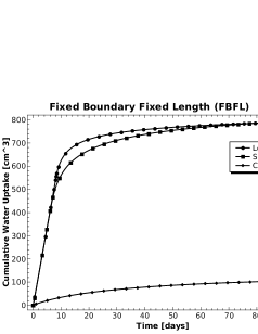
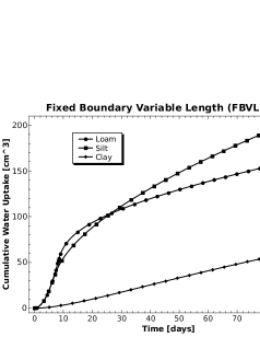
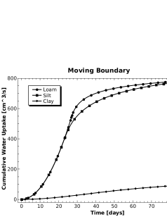
Figure 9: Cumulative water uptake time evolution for the three models, respectively fixed boundary without root growth, fixed boundary with root growth and moving boundary with the root growth.

To analyze the effect of parameter variation on model output variables, several sensitivity diagrams were made using a local approach [23]. The results are presented in Tables 4, 5, 6 and 7 as a function of the multiplicative factor of each parameter for the loam soil. The more relevant parameters are $V$ and $S_{max}$, having both positive correlation on the water uptake at 30, 60 and 90 days and negative correlation with the MUT. As for the WUMUT, $S_{max}$ has a negative correlation and $V$ has a positive correlation. $s_{0}$ has an almost constant sensitivity and always positive correlation. Therefore the experimental measurement errors on those parameters would be more amplified on the output of the model. For the silt soil there is a very similar pattern than for the loam soil. For the clay soil there are some differences. $S_{max}$ is no longer a relevant parameter and $s_{0}$ is a relevant parameter with positive correlation to the accumulative water uptake. For the MUT and WUMUT $s_{0}$ has a negative correlation. The behavior of $V$ is left unchanged with respect to the loam soil. MUT shows almost no sensitivity to $S_{max}$ but the WUMUT shows that this parameter is very relevant with positive correlation. All the sensitivities are non linear with some exceptions for $s_{0}$.

Factor	$0.5$	$1.5$	$2.0$
$U_{30}$	$-1.5\ 10^{-3}$	$1.5\ 10^{-3}$	$2.9\ 10^{-3}$
$U_{60}$	$-1.6\ 10^{-4}$	$1.6\ 10^{-4}$	$3.2\ 10^{-4}$
$U_{90}$	$-9.1\ 10^{-5}$	$8.7\ 10^{-5}$	$1.7\ 10^{-4}$
MUT	$2.1\ 10^{-3}$	$-2.1\ 10^{-3}$	$-4.2\ 10^{-3}$
WUMUT	$-7.8\ 10^{-5}$	$4.6\ 10^{-5}$	$1.1\ 10^{-4}$

Table 4: Sensitivity of the moving boundary model to the variation of the initial length $l_{0}$ for the loam soil. $U_{30}$, $U_{60}$, and $U_{90}$ are the cumulative water uptake at 30, 60 and 90 days respectively. MUT and WUMUT are the maximum uptake time and the cumulative water uptake at maximum uptake time respectively. The sensitivity is the change of the output divided by the value of the output without variation of the parameter.

Factor	$0.5$	$1.5$	$2.0$
$U_{30}$	$-1.5\ 10^{-2}$	$9.7\ 10^{-3}$	$1.7\ 10^{-2}$
$U_{60}$	$-1.0\ 10^{-2}$	$6.6\ 10^{-3}$	$1.2\ 10^{-2}$
$U_{90}$	$-7.7\ 10^{-3}$	$4.7\ 10^{-3}$	$8.1\ 10^{-3}$
MUT	$-1.4\ 10^{-2}$	$9.0\ 10^{-3}$	$1.6\ 10^{-2}$
WUMUT	$-2.8\ 10^{-2}$	$1.8\ 10^{-2}$	$3.2\ 10^{-2}$

Table 5: Sensitivity of the moving boundary model to the variation of the root radius $s_{0}$ for the loam soil. $U_{30}$, $U_{60}$, and $U_{90}$ are the cumulative water uptake at 30, 60 and 90 days respectively. MUT and WUMUT are the maximum uptake time and the cumulative water uptake at maximum uptake time respectively. The sensitivity is the change of the output divided by the value of the output without variation of the parameter.

Factor	$0.5$	$1.5$	$2.0$
$U_{30}$	$-4.5\ 10^{-1}$	$6.4\ 10^{-2}$	$8.0\ 10^{-2}$
$U_{60}$	$-1.3\ 10^{-2}$	$1.3\ 10^{-3}$	$1.5\ 10^{-3}$
$U_{90}$	$-1.1\ 10^{-3}$	$1.0\ 10^{-3}$	$2.3\ 10^{-3}$
MUT	$4.8\ 10^{-1}$	$-2.1\ 10^{-1}$	$-3.4\ 10^{-1}$
WUMUT	$8.7\ 10^{-2}$	$-6.3\ 10^{-2}$	$-1.1\ 10^{-1}$

Table 6: Sensitivity of the moving boundary model to the variation of the maximum root water uptake per unit of root length $S_{max}$ for the loam soil. $U_{30}$, $U_{60}$, and $U_{90}$ are the cumulative water uptake at 30, 60 and 90 days respectively. MUT and WUMUT are the maximum uptake time and the cumulative water uptake at maximum uptake time respectively. The sensitivity is the change of the output divided by the value of the output without variation of the parameter.

Factor	$0.5$	$1.5$	$2.0$
$U_{30}$	$-4.5\ 10^{-1}$	$1.0\ 10^{-1}$	$1.5\ 10^{-1}$
$U_{60}$	$-5.9\ 10^{-2}$	$2.5\ 10^{-2}$	$3.9\ 10^{-2}$
$U_{90}$	$-3.6\ 10^{-2}$	$1.6\ 10^{-2}$	$2.6\ 10^{-2}$
MUT	$4.1\ 10^{-1}$	$-1.8\ 10^{-1}$	$-2.9\ 10^{-1}$
WUMUT	$-7.3\ 10^{-3}$	$4.3\ 10^{-3}$	$7.4\ 10^{-3}$

Table 7: Sensitivity of the moving boundary model to the variation of the maximum root water uptake per unit of root length $S_{max}$ for the loam soil. $U_{30}$, $U_{60}$, and $U_{90}$ are the cumulative water uptake at 30, 60 and 90 days respectively. MUT and WUMUT are the maximum uptake time and the cumulative water uptake at maximum uptake time respectively. The sensitivity is the change of the output divided by the value of the output without variation of the parameter.

Mass conservation implies that the total water volume must be the same at the beginning and at an arbitrary time of the simulation. Since the water can only be in the soil or inside the root, therefore the total water volume $\left(T\left[cm^{3}\right]\right)$ at time $t$ would be

$$T(t)=U(t)+W(t)$$ (38)

with $U(t)$ and $W(t)$ defined as in equations (14) and (16) respectively. At the beginning of the simulation the cumulative water uptake is null, therefore the total water is the water in soil. With the above considerations the change of the cumulative water uptake plus the water remaining in the soil minus the initial water content $(W(t)+U(t)-W(0))$ as a function of time was calculated. For the FBVL model the mass balance cannot be done because to compute the water remaining in soil, the operation must be done with pressure head profiles as a function of time which has been calculated in fixed domain, but this result must be compared with the cumulative uptake by a growing root, which has been calculated integrating in a variable domain. The results of those calculations are shown in Figure 10. It shows that there is an effect of water mass loss for the moving boundary model that is not present on the fixed boundary model. There are two possible causes for this mass loss. The first cause is the assumption of total volume constant in the formulation of the model, reflected in the moving boundary formula $\left(R(t)=R_{0}\sqrt{\frac{l_{0}}{l(t)}}\right)$, i.e., the volume that is kept constant is the soil plus root volume, being the volume occupied by the root is $V_{R}=\pi s_{0}^{2}l(t)$. Then the soil volume is the total volume minus the root volume, therefore the root occupies a bigger fraction of the total volume as time increases (see Figure 1). The water content in the volume of soil removed by the root is not taken into account in the calculation of the water in the soil volume $(W(t))$. This means, in other words, that, for the model, the root is “eating” the soil, and the water which is in that portion of the soil. The second cause is the numerical errors. This case is similar for both models and does not contribute a large mass loss. An important remark is that the FEM is used to solve the water potential $(\Psi)$, not the water content $(\theta)$, on a discretized space with a finite precision, and cumulative errors could lead to a mass creation or loss depending of the parameters. Figure 10 shows the soil volume loss effect plus the water mass loss due to the used numerical method in each integration step. In each soil for the moving boundary model the water loss is around $1\%$ of the total water. For the clay soil the total loss is around $15\%$ of the total water uptake, while for the other soils the loss is less than $2\%$. The water loss for the fixed boundary model is negligible compared with the total water or the cumulative water uptake.

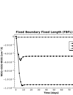
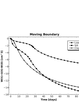
Figure 10: Water mass balance $(W(t)+U(t)-W(0))$ versus time $(t)$ for the values shown in Table 2 for the FBFL and the Moving Boundary models. The total water is the cumulative water uptake plus the water remaining in the soil, the initial water is the total water at the start of the simulation.

4 Conclusions

An important remark is that all the results presented before are computed for a single plant, in a fixed soil volume with initial soil water content equal for all simulations, to compare the effect of the different soils on the water uptake. The parameters used represent traits of the plant. $V$ can be regarded as the response to nutrient and water uptake and is influenced by the plant genetics. $S_{max}$ is linked to atmospheric factors and to genetic variation. $s_{0}$ is the constant root radius. $l_{0}$ is a growing stage trait, changes in it only means a change in the development of the rooting system when the simulation begins.

There is a large difference in behaviour among the silt and loam soil on one hand and the clay soil on the other hand. Initial pressure head (Table 3) and pressure head profiles are different (Figures 4, 5 and 6), and instantaneous water uptake is much smaller (Figures 7 and 8). This can be explained in terms of the water uptake function $(G(\Psi))$. For the clay soil the water uptake function is on the linear regime (zone (b) of Figure 2) and the water potential is sharply decreasing (drying the soil) at the root-soil interface. Once the time variation of the water potential at the interface is stabilized the root growth has the dominant effect on uptake and the curve is similar to the other curves, although it shows a non linear behavior.

From Figure 10, the mass balance is not exactly zero owing to the numerical method used. For the FBFL model the differences are due to numerical errors only and are very low compared with the water volume loss on the moving boundary model. The mass variation is produced on the high instantaneous uptake zone, this is a known flaw of the finite elements method. The moving boundary model has a higher mass variation compared with the FBFL model by the accumulation of two factors, numerical errors as in FBFL model, and a soil volume loss effect. The soil volume loss effect is introduced by the assumption of constant total volume (roots grows at the expense of a decrease in the soil volume), which is reflected on the formula of the moving boundary (12). For the moving boundary model the differences on the total values of water mass loss by a soil volume loss effect and numerical errors are due to the different variations of the soil water contents. The clay soil has low available water (see Table 3), but the total water mass loss is similar to the other soils, and it represents about $10\%$ of the initial total water. The assumptions that generate the soil volume loss effect should be revised when soils for which the initial potential is on the linear zone (i.e., low water availability) are studied. The water mass loss is consistent with the model assumptions, and the numerical induced errors are low compared to the water uptakes $(<15\%$ for clay soils, and $<2\%$ for the other soils). There are two main actions to avoid the volume loss effect. The first one is to keep the soil volume constant and not the root-soil volume. The second one is to evaluate the mass loss and put it back into the soil using a source function or a modification of the boundary conditions. Each procedure will have its advantages and disadvantages, but, since the water loss is very low compared with the water uptake for the studied cases, the revision is left for a specific work on low initial available water.

The obtained results shows a global consistency with the structure of soils studied, becoming a valuable tool to study the water uptake in a more complex situation (for example when the effect of a variable evapotranspiration on $S_{max}$ is considered).

Obviously, the results would change when plants not growing in pots but in the field (in this case equation (12) is invalid) are considered. Here is necessary to develop a new rooting development function $R(t)$. One change in this model to be useful in a field situation is the use of a coordinate representing the depth and water transport by gravity. Here $R(t)$ should incorporate the root architecture. Moreover, since this is a first approach a simple water uptake function has been used. This function could be changed to a more complex function [24, 25]. Moreover the effect of $V$ and $S_{max}$ could change substantially after the first 30 days in field conditions, since there will be circadian and climatic effects that will alters the root water uptake function $(G)$, and the evapotranspiration will be a parameter to be measured or calculated before the simulation.

The differences among models with and without root growth can bee seen in figures 8 and 9. The dynamics of water uptake for the fixed boundary models are very different from those of a moving boundary model. The maximum instantaneous water uptake is achieved much faster for the fixed boundary model. Also a difference in the beginning and end of the simulation for the values of the instantaneous water uptake can be observed, while for the FBFL and the moving boundary model the instantaneous water uptake reaches values close to zero as time goes by, is not clear that the FBVL model has the same behavior. This difference is because the influx on root surface is computed for a single root in a fixed domain and the cumulative uptake by the growing root is calculated using these influxes. From a physical point of view, to compute the cumulative uptake influxes calculated in a variable domain should be used. Therefore the mass balance cannot be calculated for the FBVL. For those considerations of mass conservation the FBVL approach should be avoided on water uptake models.

5 Acknowledgments

The authors would like to acknowledge the valuable suggestions of Guillermo G. Weber from the University of Texas at Brownsville, and Sergio Preidikman from Universidad Nacional de Córdoba (UNC) for the implementation of the FEM. This work was supported in part by PIP N 18/C362 from SECyT-UNRC and PIP Nº 0534 from CONICET-UA, Argentina. The authors would like to acknowledge the valuable suggestions made by the anonymous referees to this work.

Appendix A Deduction of simplified total water uptake

The formula for water uptake given by [15] is

$$U(t) = l_{0}\int_{0}^{t}G(\Psi(s_{0},\tau))d\tau$$ (39)

$$+\int_{0}^{t}\left(\int_{\tau}^{t}G(\Psi(s_{0},\tau))d\tau\right)\dot{l}(\tau)d\tau,$$

the second integral on the right side can be reduced, by a parts integration, into

$$U(t) = l_{0}\int_{0}^{t}G(\Psi(s_{0},\tau))d\tau$$ (40)

$$+\left.\left(\int_{\tau}^{t}G(\Psi(s_{0},\tau))d\tau\right)l(\tau)\right|_{0}^{t}-\int_{0}^{t}\left(-G(\Psi(s_{0},\tau))\right)l(\tau)d\tau,$$

$$U(t) = l_{0}\int_{0}^{t}G(\Psi(s_{0},\tau))d\tau$$ (41)

$$-\left(\int_{0}^{t}G(\Psi(s_{0},\tau))d\tau\right)l(0)+\int_{0}^{t}G(\Psi(s_{0},\tau))l(\tau)d\tau$$

Therefore the final result is

$$U(t) = \int_{0}^{t}G(\Psi(s_{0},\tau))l(\tau)d\tau$$ (42)

References

- [1] I. Cowan, Transport of water in the soil-plant-atmosphere system, Journal of Applied Ecology 2 (1) (1965) 221–239.
- [2] W. Gardner, Dynamic aspects of water availability to plants, Soil Science 89 (1960) 63–73.
- [3] T. Van den Honert, Water transport in plant as a catenary process, Discuss. Faraday Soc. 3 (1948) 146–153.
- [4] R. Feddes, H. Hoff, M. Bruan, T. Dawson, P. de Rosnay, P. Dirmeyer, R. Jackson, P. Kabat, A. Kleidon, A. Lilly, A. Pitman, Modelling root water uptake in hydrological and climate models, Bulletin of the American Meteorogical Society 82 (2001) 2797–2809.
- [5] D. Hillel, Aplications of soil physics, Academic Press, New York, 1980.
- [6] F. Molz, Models of water transport in the soil-plant system: a review, Water Resources Research 17 (5) (1981) 1245–1260.
- [7] A. Guswa, Soil-moisture limits on plant uptake: An upscaled relationship for water-limited ecosystems, Advances in Water Resources 28 (2005) 543–552.
- [8] M. Puma, M. Celia, I. Rodriguez-Iturbe, A. Guswa, Functional relationship to describe temporal statistics of soil moisture averaged over different depths, Advances in Water Resources 28 (2005) 553–566.
- [9] E. Personne, A. Perrier, A. Tuzet, Simulating water uptake in the root zone with a microscopic-scale model of root extraction, Agronomie 23 (2003) 153–168. doi:10.1051/agro:2002081.
- [10] T. Roose, A. Fowler, A model for water uptake by plant roots, Journal of Theoretical Biology 228 (2004) 155–171.
- [11] E. Wang, C. Smith, Modelling the growth and water uptake function of plant root systems: a review, Australian Journal of Agricultural Research 55 (2004) 501–523.
- [12] J. Wu, R. Zhang, S. Gui, Modelling soil water movement with water uptake by roots, Plant and Soil 215 (1999) 7–117.
- [13] J. Reginato, M. Palumbo, D. Tarzia, C. Bernardo, I. Moreno, Modelling nutrient uptake using a moving boundary approach. comparison with the barber-cushman model, Soil Science Society of America Journal 64 (2000) 1363–1367.
- [14] M. Van Genuchten, A closed-form equation for predicting the hydraulic conductivity of unsaturated soils, Soil Science Society of America Journal 44 (1980) 892–896.
- [15] J. Reginato, D. Tarzia, An alternative formula to compute the nutrient uptake, Comm. in Soil Sci and Plant An. 33 (5&6) (2002) 821–830.
- [16] J. Reddy, An introduction to nonlinear finite element analysis, Oxford University Press, New York, 2004.
- [17] P. Solutions, Flexpde, http://www.pdesolutions.com/.
- [18] J. T. Ritchie, Soil-water availability, Plant and Soil 58 (1981) 327–338.
- [19] R. Feddes, P. Kowalik, H. Zaradny, Simulation of field water use and crop yield, Centre for Agricultural Publishing and Documentation, Wageningen, Netherlands, 1978.
- [20] J. Kelly, S. Barber, G. Edwards, Modelling magnesium phosphorus and potassium uptake by loblolly pine seedling using a barber-cushman approach, Plant and Soil 139 (1992) 209 – 218.
- [21] N. Claasen, S. Barber, Simulation model for nutrient uptake from soil by a growing plant root system, Agronomy J. 68 (1976) 961–964.
- [22] J. H. Cushman, An analytical solution to solute transport near root surfaces for low initial concentration: I equation development, Soil Sci. Soc. Am J 43 (1979) 1087–1090.
- [23] A. van Griensven, T. Meixner, S. Grunwald, T. Bishop, M. Diluzio, R. Srinivasan, A global sensitivity analysis tool for the parameters of multi-variable catchment models, Journal of Hydrology 324 (2006) 10–23.
- [24] J. Vrugt, M. Wijk, J. Hopmans, J. Simunek, One-, two-, and three-dimensional root water uptake functions for transient modelling, Water Resources Research 37 (10) (2001) 2457–2470.
- [25] K. Li, R. De Jong, M. Coe, M. Ramankutty, Root-water-uptake based upon a new water stress reduction and an asymptotic root distribution function, Earth Interactions 10 (14) (2006) 1–22.