Geometric proof for normally hyperbolic invariant manifolds
Maciej J. Capiński111Research supported by the Polish National Science Center Grant 2012/05/B/ST1/00355mcapinsk@agh.edu.plAGH University of Science and Technology, al. Mickiewicza 10, 30-059 Kraków, Poland
Piotr Zgliczyński222Research supported by the Polish National Science Center Grant 2011/03/B/ST1/04780umzglicz@cyf-kr.edu.plJagiellonian University, ul. prof. Stanisława Łojasiewicza 6,
30-348 Kraków, Poland
Abstract
We present a new proof of the existence of normally hyperbolic manifolds and their whiskers for maps. Our result is not perturbative. Based on the bounds on the map and its derivative, we establish the existence of the manifold within a given neighbourhood. Our proof follows from a graph transform type method and is performed in the state space of the system. We do not require the map to be invertible. From our method follows also the smoothness of the established manifolds, which depends on the smoothness of the map, as well as rate conditions, which follow from bounds on the derivative of the map. Our method is tailor made for rigorous, interval arithmetic based, computer assisted validation of the needed assumptions.
keywords:
Invariant manifolds, normal hyperbolicity
MSC:
[2010] 34C45, 34D35, 37D10
††journal: Journal of Differential Equations
1 Introduction
The goal of our paper is to present a geometric proof of the existence of
normally hyperbolic invariant manifolds (NHIMs) for maps, in a vicinity of
an approximate invariant manifold. There are four important features of our
approach: 1) we do not assume that the given map is a perturbation of some
other map for which we have a normally hyperbolic invariant manifold, 2) we
do not require that the map is invertible, 3) the assumptions can be
rigorously checked with computer assistance if our approximation of the
invariant manifold is good enough 4) our method does not require high order
smoothness. From our proof follows the high order smoothness of the
manifolds (provided that the map is suitably smooth), but it is enough to
consider bounds for the proof of their existence.
In the standard approach to the proof of various invariant manifold
theorems, all considerations are done in suitable function spaces or
sequences spaces. Moreover the existence of the invariant manifold for
nearby map (or ODE) is usually assumed, see for example [4, 16, 20]
and the references given there. Typically these proofs do not give any
computable bounds for the size of perturbation for which the invariant
manifold exists.
Our result is in similar spirit to a number of results for establishing
invariant manifolds that have recently emerged, which assume that there
exists a manifold that is ‘approximately’ invariant, and provide conditions
that ensure the existence of a true invariant manifold within a given
neighborhood. In [1] Bates, Lu and Zeng present such approach within
a context of semiflows, which makes their method general and applicable to
infinite dimensional systems and PDEs. Compared to [1] our results
is more explicit. Contrary to [1], where main theorems about NHIM
require that some constants are sufficiently small depending on other
constants, in our main theorem we just have several explicit inequalities
between pairs of constants. In [3, 11, 12, 13, 14] Calleja, Celletti,
Haro, de la Llave, Figueras, Fontich and Sire provide a framework and
results of establishing existence of whiskered tori with quasi periodic
dynamics, which is suitable for computer assisted validation. Our approach
however allows for more general dynamics. All above proofs are based on
constructions in suitable function spaces.
In contrast to the above mentioned approach, in our method the whole proof
is made in the phase space. This method is not entirely new. For example, a
similar approach is adapted in the proof of Jones [17] in the context of
slow-fast system of ODEs. Jones though considered a perturbation of a
normally hyperbolic invariant manifold. In [5, 8] an approach in the
same spirit as in this paper has been applied to establish existence of
topologically normally hyperbolic invariant manifolds. These results are
based on topological arguments and do not establish the smoothness and the
foliations of the invariant manifolds. Similar approach has been applied by
Berger and Bounemoura [2], where persistence and smoothness of
invariant manifolds is established using geometric and topological methods.
The result relies though on a perturbation of a normally hyperbolic
invariant manifold.
The method in this paper is based on two types of conditions. The first are
the topological conditions, which we refer to as ‘covering relations’. These
ensure that we have good topological alignment of the coordinates of the set
within which we establish the existence of the manifold. The second type of
conditions are based on the first derivative of the map and we refer to
these as the ‘rate conditions’. Our rate conditions are in the same spirit
to those of Fenichel [9, 10]. They measure the strength of the
hyperbolic contraction and expansion (within a neighborhood in which we
search for our manifold), in comparison to the dynamics on the normal
coordinates. The stronger the hyperbolicity is, the higher is the order of
the smoothness that can be established.
Our construction of the manifolds follows from a graph transform type
method. We prove that the manifolds emerge from passing to the limit of
graphs in appropriate coordinates. This construction follows primarily from
the covering conditions. To prove that the manifolds are Lipschitz, we show
that our graphs are contained in cones (this is the approach that was taken
in [8]). The novelty of this paper lies in the proof of the higher
order smoothness. In our proof, this follows from establishing appropriate
cone conditions for the graphs. We define higher order cones, which span
around Taylor expansions of the graphs. We prove that these cones are
preserved as we iterate the graphs. (Verification of this fact follows from
our rate conditions.) We then show that higher order cone conditions imply
higher order smoothness of the graphs, and that this smoothness is preserved
as we pass to the limit.
We emphasize that in order to apply our method it is sufficient have a good
guess on the position of the manifold and good estimates of the first
derivative of the map. We do not require any estimates on its higher order
derivatives. It is sufficient that we know that the map is appropriately
smooth, and that the first derivative implies our rate conditions.
We believe that this approach is very well suited for computer assisted
(rigorous, interval arithmetic based) validation of the needed assumptions.
Similar approach has already been successfully applied in [5, 8] in
the setting of the rotating Hénon map, in [6] to establish the
center manifold in the restricted three body problem, in [7] in the
setting of a driven logistic map or in [21] to establish a hyperbolic
attractor in the Kuznetsov system. All these results follow from
verification of cone conditions based on the estimates of the derivative. We
believe that such estimates also imply rate conditions, hence the method
from this paper can easily be used to establish smoothness and fibration of
the manifolds. At present moment it appears that of approaches to NHIMs
mentioned earlier in the introduction only the one based on the
parameterization method [3, 11, 12, 13, 14] are ready for computer
assisted proof. This method is however restricted by the requirement of the
quasi-periodic dynamics on the invariant torus.
The paper is organized as follows. After preliminaries introducing basic
notations in Sections 3 we state our main result for
the case of the torus. Sections 4–10
contain the proof of our main result for the torus. In Section 11 we show to how our construction can be carried over from the
torus to arbitrary compact manifold. We decided to work first with the torus
rather then a general manifold, because in that case we can have a global
coordinate chart and the main ideas are not mixed with the technicalities
connected with different charts. In Section 12 we apply our
method to the rotating Hénon map.
2 Preliminaries
2.1 Notations
For a point we shall use to denote the projection
of onto the coordinate. We use a notation for a ball of
radius in , centered at . To simplify notations we
shall write . For a set we
shall write for closure of and for the
boundary of . Throughout the work, the notation will stand for the Euclidean norm, unless explicitly stated otherwise. For
a set and a continuous function (homotopy) , for we shall write for .
Definition 1
Let be a function. We
define the interval enclosure of the derivative on , as a set , defined as
Definition 2
Let be a linear map. Let be any norm on , then we define
For an interval matrix we set
2.2 Taylor formula
In this section we quickly set up the notations for the Taylor formula. Let
The -th derivative of at is a symmetric -linear operator. On
the basis it is defined as
Using the following multi-index notation
we can write out the value of on the diagonal as
The above formula is convenient to formulate the multi-dimensional version
of the Taylor formula:
where stands for the Taylor expansion of order
and the reminder can be computed in the integral form
For and
a set we define
3 Main results
The goal of this section is to set up the structure for our NHIM, which will
be diffeomorphic with a manifold . To make the setup as simple as
possible we will focus on the special case where is a torus. This
will simplify notations in many of the arguments, since we will not need to
work with various local charts. We shall prepare the setup though in a way
that will allow for a straightforward generalization to an arbitrary
manifold without boundary. This will be done in section 11.
3.1 Definitions and setup
In the simple situation when is an -dimensional torus, we are
in a convenient situation, since we have a covering
which gives us the set of charts being the restriction of to
balls in , which are small enough so that is a homeomorphism on its image. We introduce a
notation for a radius such that is a homeomorphism onto its image. When is a
torus, we can simply take Introducing the
notation here though will simplify our future discussion in
section 11, where we generalize the results.
Let and denote by the set
where stands for a closed ball of radius , centered
at zero, in . We consider a map, for ,
Throughout the paper we shall use the notation to denote
points in . This means that notation will stand for points on , notation for points in , and for points
in . We will write as ,
where stand for projections onto , and , respectively. On we will use the Euclidian norm.
In view of the further generalization to arbitrary manifold let us stress
that our set can be thought as a subset of the trivial vector bundle .
Definition 3
The set of points which are in the same good chart with point will
be denoted by
Let , and let us define
Remark 4
Throughout the work, the is a fixed
constant. We shall later see that is associated with Lipschitz bounds on
the established manifolds (hence the choice of notation).
The key to the naming of the constants is the following:
1.
, - the constants describing lower
bound on the expansion in the unstable or center-unstable directions.
2.
, - the constants describing upper
bound for contraction constant in the stable or center-stable direction.
3.
The number or as second lower index is used according to the
following rule: , when both partial derivatives are of the same component
of , for example in , while is used
the differentiation is done with respect to the same block of variables of
various components of .
4.
, , , are the
expansion bounds and , , ,
are the contraction bounds, that are used for the establishing of smoothness
of invariant manifolds and their fibres.
5.
, are more stringent bounds (i.e. ). They are used to ensure lower bounds on
the expansion on the and coordinates.
Definition 5
We say that satisfies rate conditions of
order if
are strictly positive, and for all holds
(1)
(2)
(3)
(4)
We say that satisfies rate conditions of order zero, if only (1)–(2) are satisfied.
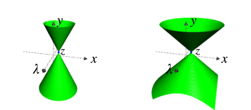
We introduce the following notation:
(5)
(6)
We shall refer to as a stable cone of slope at , and to as an unstable cone of slope at . The cones are depicted
in Figures 1, 2.
Figure 1: The stable cone for on the left, and on the right.
Remark 6
For any and with we see that
This means that
for . Similarly, for
In other words, intersections of unstable (stable) cones with are
contained in sets on which we can use a single chart .
Definition 7
We say that a sequence is a (full)
backward trajectory of a point if and for all
Definition 8
We define the center-stable set in as
Definition 9
We define the center-unstable set in as
Definition 10
We define the maximal invariant set in as
Definition 11
Assume that . We define the stable fiber
of as
Definition 12
Assume that . We define the unstable fiber
of as
for any such backward trajectory
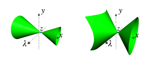
Figure 2: The stable cone for on the left, and on the right.
The definitions of and are related to cones, which
is a nonstandard approach, the standard one is through convergence rates. We
will show that our definition implies the convergence rate as in the
standard theory.
Under our assumptions it will turn out that is injective on .
Therefore the backward orbit in the definition of is unique.
Definition 13
We say that satisfies backward cone conditions if the
following condition is fulfilled:
If and then
Remark 14
The assumption that satisfies backward cone conditions will turn out to
be necessary in order to ensure that the established NHIM is a graph over . After formulating our main Theorem 16, we follow up
with Examples 21, 22, in which we
demonstrate that without backward cone conditions the result cannot be
obtained.
For we define the following sets:
Definition 15
We say that satisfies covering conditions if for any
there exists a , such that the
following conditions hold:
For , there exists a homotopy
and a linear map which satisfy:
1.
2.
for any ,
(7)
(8)
3.
,
4.
In the above definition a reasonable choice for will be . In fact any point sufficiently close to will be also good.
3.2 The main theorem
Theorem 16
(Main result) Let and be a map. If
satisfies covering conditions, rate conditions of order and backward
cone conditions, then and are
manifolds, which are graphs of functions
meaning that
Moreover, is an injection, and are Lipschitz
with constants , and is Lipschitz with the constant . The manifolds and intersect
transversally, and .
The manifolds and are foliated by invariant fibers and . The and are graphs of functions
meaning that
The functions and are Lipschitz with constants . Moreover,
and if is the unique backward trajectory of
in , then
Observe that bound on gives
us lower bounds for the Lipschitz constants for functions , , , , which is clearly an overestimate for the case when is our NHIM. This lower bound is a
consequence of choices we have made when formulating Theorem 16,
as we did not want to introduce different constants for each type of cones,
plus several inequalities between them. However, below we give conditions
which allow to obtain better Lipschitz constants.
Theorem 17
Let and
(9)
(10)
If assumptions of Theorem 16 hold true and also , then the function from Theorem 16 is Lipschitz
with constant
Theorem 18
Let and
If assumptions of Theorem 16 hold true and also , then the function from Theorem 16 is Lipschitz
with constant
Theorem 19
Let and
If assumptions of Theorem 16 hold true and also , then the function from Theorem 16 is Lipschitz with
constant .
Theorem 20
Let and
If assumptions of Theorem 16 hold true and also , then the function from Theorem 16 is Lipschitz with
constant .
3.3 Comments on the inequalities and examples
Let and stand for the complements of and respectively. We now comment about what
various inequalities in Definition 5 of rate
conditions mean and what they are needed for:
1.
: the forward invariance of
(Corollary 34). : the expansion in for - coordinate (Lemma 36). This is
needed for the proof of the existence of (Section 7).
2.
: the forward invariance of (Corollary 35). : the
contraction in -direction in (Lemma 37). This is needed for the proof of the existence of (Section 6).
We now give two examples which show that in the absence of the backward cone
condition, the invariant set might not be a graph over .
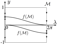
Example 21
Consider a Möbius strip depicted in
Figure 3. The Möbius strip is parameterised by , with and . The two vertical edges which are glued
together are depicted with arrows.
Let be a constant. We consider a map
On the unstable coordinate , is simply a linear expansion. The stable
coordinate is the vertical coordinate on . The coordinates and are decoupled. Intuitively, on the map does the following. It projects
into a horizontal circle, and then stretches it and wraps twice around as in Figure 3. For such a map all assumptions
of Theorem 16 are fulfilled, except for the backward cone
conditions. We see that in the absence of the backward cone conditions, the
invariant manifold can be a set which is not a graph over .
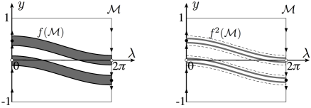
Example 22
We can modify Example 21 slightly to
obtain a more interesting result. Assume that and consider
The difference is that instead of collapsing completely, we
contract in the coordinate. Then will be the set
depicted on the left plot of Figure 4. The second iterate is
shown in the right plot of Figure 4. We thus see that the
invariant set has a Cantor structure.
Above examples are artificial. Similar features though can be found for
instance in the Kuznetzov system (see [18],[21]), where we have
a hyperbolic invariant set in , which has a Cantor set
structure. By adding the assumption that satisfies backward cone
conditions we rule out such cases, and establish NHIMs that are graphs over .
4 Cone evolution
In this section we introduce the notion of ”higher order cones”. These will
be used to control the smoothness of established manifolds. The section
contains auxiliary results. The construction of the manifolds is performed
in Sections 6, 7 and 8.
4.1 Unstable cones
In this section we introduce the cones. We formulate the results in a
setting where we have two coordinates and , instead
of the three coordinates from Section 3. This is because the results are formulated in more
general terms. Later, we shall apply these taking and (or, in other instances, and ) in our construction of the manifolds. Thus, the
subtle change of font in and plays an important
role.
Let
be a polynomial of degree .
Definition 23
We define an unstable cone of order at spanned on
with a bound as a set of the form
(11)
Remark 24
We emphasize that the index in is
important since it stands for the order of the cone. Cones of order
are always associated with polynomials of degree . Let us also observe
that if we take a polynomial (of degree zero) , then for and the cones defined
in (6) and (11) are the same:
For we define
The above defined cones are devised to control higher order derivatives of
functions. The following lemmas explain this relation.
Lemma 25
Assume that is a function. Let , . Then
there exists a , such that
The following theorem shows that, under appropriate assumptions, cones of
order map to other cones, with the same bound .
Theorem 28
Let be a convex bounded neighborhood of zero and assume that is a map
satisfying and . Assume that we
have two polynomials with coefficients bounded by , such that
(17)
If for , and
(18)
and
(19)
then there exists a constant , such that for any there exists a such that
Moreover, if for some holds , then depends only on and .
We define a stable cone of order at spanned on with a bound as a set of the form
For we define
and we also denote complements of the cones as
Mirror results to Lemmas 25, 26 can be formulated for stable cones:
Lemma 30
Assume that is a function. Let , . Then
there exists , such that
for and
Lemma 31
Assume that is a function. Let and assume that there exists , such that
where and Then there exists a
constant (which depends only on ), such that for any
Since proofs of Lemmas 30, 31 follow from mirror arguments to the proofs of
Lemmas 25, 26, we omit
their proofs.
We now give the following theorems, which are in similar spirit to Theorem 27, 28. The difference
is that they concern images of complements of cones (and not images
of the cones themselves, as is the case in Theorems 27, 28.)
Theorem 32
Let
be a convex neighborhood of zero and assume that is a map satisfying . Assume that
for
(20)
(21)
and
(22)
then
Proof. The result follows from Theorem 27. Details are
given in F.
Theorem 33
Let be a convex bounded neighborhood of zero and assume that is a map
satisfying and . Assume that we
have two polynomials with coefficients bounded by , such that
If for , and
and
(23)
then there exists a constant , such that for any there exists
such that
Moreover, if for some holds , then depends only on and .
We now return to the setting in which we have three coordinates . Recall that in these coordinates stable cones and unstable cones were
defined using (5–6). In
addition we define center-stable and center-unstable cones as
respectively.
Observe that and . We see that and as defined above are not contained in domain of single good
chart. However we will always take intersections of these cones with the
domain of a good chart.
In this section we introduce the notion of discs. These will be the building
blocks for the construction of our invariant manifolds.
Definition 40
We say that a continuous function is a
horizontal disc if for any
(24)
Definition 41
We say that a continuous function is a
vertical disc if for any
(25)
By Remark 6, we see that any horizontal or vertical
disc can be contained in a set on which we can use a single chart. This fact
will prove important in Section 11 where we reformulate our
results for more general .
In our former works [8, 22] the disks as defined above where said to
satisfy cone conditions.
Definition 42
We say that a continuous function is a center-horizontal disc if for any
and
(26)
Definition 43
We say that a continuous function is a center-vertical disc if for any
and
(27)
Lemma 44
Assume that is
a horizontal disc. If satisfies the covering conditions and the rate
conditions of order , then there exists a horizontal disc such that . Moreover, if and
are , then so is .
The disc from Lemma 44 is a graph transform
of . From now on we shall use the notation instead
of .
Lemma 45
Assume that is a center-horizontal disc. If satisfies the
covering conditions, backward cone conditions and the rate conditions of
order , then there exists a center-horizontal disc such that
From now on we shall use the notation instead of for the disc from Lemma 45.
6 Center-unstable manifold
In this section we prove the existence and smoothness the manifold
from Theorem 16. The proof follows from a graph transform type
method, in which we take successive iterates of center-horizontal discs, and
these converge to the center unstable manifold.
We start with the following lemma, which establishes the existence of .
Lemma 46
Assume that satisfies covering conditions, backward cone
conditions and rate conditions of order . Let be the
sequence of center-horizontal discs defined as , for . Then converge
uniformly to a center-horizontal disc , where
Moreover
Proof. We use a notation . We will show that
is a Cauchy sequence in the supremum norm, which converges to .
Let us fix . For any , since is center-horizontal disk, there exists a finite
backward orbit , such that
From the backward cone condition it follows that for any points for are in the same chart and
Since condition (30)
establishes uniform convergence of to , moreover also the
backward orbits form a Cauchy sequence and converge to full backward orbit
of .
From the above it follows also that converge uniformly to a
continuous function .
Assume now that we have a that has a full backward trajectory in . We need to show that for some . Let for . We
will show that . Since ,
Then for the backward trajectory of , by the backward cone conditions,
Passing to the limit in the cone condition (26) for one can see that
Since is invariant under , by Corollary 35 we obtain (26) for Thus is a center-horizontal disc.
Lemma 47
Assume that is and satisfies covering
conditions, backward cone conditions and rate conditions of order .
Let . Let be the sequence of center-horizontal discs
defined as , for . Assume that are and
that for any with
independent of . If the order of the rate conditions is
greater or equal to , then for a constant independent of .
Proof. Let us fix . Our aim will be to show that is bounded and that the bound is
independent of . Let be any chosen point from and let be a sequence such that
for . Note that
For let be a polynomial of degree ,
defined as
Observe that since for independent from , the polynomials have a
uniform bounds for their coefficients, which is independent from and . Since we also see that for
Since are Lipschitz with a constant
Let us consider coordinates and
let, , and . Then, from Theorem 28, for
sufficiently large and sufficiently small
(31)
Note that the choice of and does not depend on . Since is a flat disc, we have
If satisfies the assumptions of Theorem 16, then the manifold is
Proof. Let be the sequence of center-horizontal discs defined as , , for . By Lemma 45, we know that are . By Lemma 46 we know that they converge uniformly to
We need to show that smoothness is preserved as we pass to the limit.
Since are Lipschitz with a constant , we see that , where is
independent of . Rate conditions of order , imply rate conditions of
order for ; in particular for . Hence, by Lemma 47 we obtain that .
Applying Lemma 47 inductively we obtain that , with
independent of . This implies that derivatives of of
order smaller or equal to are uniformly bounded and uniformly
equicontinuous. This by the Arzela Ascoli theorem implies that and their derivatives of order smaller or equal to converge
uniformly. Thus is , as required.
Lemma 49
If satisfies the assumptions of Theorem 16, then is injective.
Proof. If and then and by the backward cone conditions hence by Remark 6, and are in the same chart. This means that it is enough to show that for
any which are on the same chart, we can not have and .
Proof of Theorem 19.
The result follows from showing that
(33)
By definition of (33) clearly holds for To prove (33) for all , one
can inductively apply the same argument as the one from the proof of Theorem 32 (page F). Passing with to infinity we obtain our claim.
7 Center-stable manifold
The goal of this section is to establish the existence of the center stable
manifold from Theorem 16.
We will represent as a limit of graphs of smooth functions. Here we
take the first step in this direction. For any and we consider the
following problem: Find such that
(34)
under the constraint
(35)
From Lemma 44 it follows immediately that this problem
has a unique solution which is as smooth as .
Lemma 50
Let be given by . Then is a center vertical disc and the sequence
converges uniformly to . Moreover, is a center vertical
disk in , such that
(36)
Proof. To show that is a center vertical disc, we have to prove that if , then . We will
argue by the contradiction. Assume that , which implies . Then from Lemma 36, applied
inductively, it follows that
This contradicts (34). This establishes that are
center vertical discs.
To prove the uniform convergence of we show the Cauchy condition for
this sequence. Let . We have , hence by Lemma 36
Since
we obtain
This, since , proves uniform convergence of to some
disk . Observe that
because for each and
(37)
Fixing in (37) and passing to the limit with ,
we obtain that for all .
We now need to show that we can not have a point such that Since by
Lemma 36, for all
Since and since we see that , which implies
that .
Condition (36) is an immediate consequence of (7), since if we had with then .
We finish by showing that is a center-vertical disc. We have already
established that are center-vertical discs. Passing to the limit,
for any ,
(38)
The condition (27) follows from Corollary 34 by the following argument. If we had a point in such that
Let Let be the sequence of
center-horizontal discs defined in Lemma 50. Assume
that are and that for any with independent of . If
satisfies rate conditions of order , then for a constant independent of .
Proof. The proof goes along the same lines as the proof of Lemma 47. We shall write .
Since follows from the solution of problem (34)
(40)
Let us fix . Our aim will be to show that is bounded and that the bound is
independent of . Let be any chosen point from and let be a sequence defined as
Since for
independent from , the polynomials have a uniform
bounds for their coefficients, which is independent from and . Since are center vertical discs, are Lipschitz with a
constant hence
Let us consider coordinates and
constants , and . By (40) we see that for
From Theorem 33, for sufficiently large and
sufficiently small
(41)
Note that the choice of and does not depend on . Since is a flat disc, we have
If satisfies the assumptions from Theorem 16, then the manifold is
Proof. The functions are and uniformly Lipschitz with
constant . The fact that smoothness is preserved as we pass to
the limit follows from Lemma 51 and mirror arguments
to the proof of Lemma 48.
Proof of Theorem 20.
We shall write Our
first aim is to show that for
(43)
Let , and suppose that (43) does not hold.
Then From Theorem 27 (taking , and
in place of ) we see that for By the same argument as the one in
the proof of Lemma 36 (on page H) we have
which contradicts the fact that by definition of , . Thus we
have proven (43).
The claim follows by passing with to infinity in (43).
8 Normally hyperbolic manifold
In this section we establish the existence of the normally hyperbolic
invariant manifold from Theorem 16. Throughout the section we
assume that assumptions of Theorem 16 are satisfied.
Lemma 53
For any there
exists a point with .
Proof. Let be
defined as
By the Brouwer fixed point theorem, there exists a such that . We see that . Let and . Since
hence
clearly lies on .
Lemma 54
Let , then and intersect transversally at .
Proof. The manifold is parameterized by and is parameterized by . Let
We need to show that
(44)
We see that is equal to the range of the matrix
We will show that
is invertible. If for , then
which since and are Lipschitz with constant implies
that and in turn that . Since is invertible, it is evident
that the rank of is which implies (44).
Lemma 55
The is a manifold, which is a
graph over of a function , which is Lipschitz with a constant .
Proof. From Lemma 53 it follows that for every the set is nonempty. We will show that this set consists
from one point and is a function satisfying the
Lipschitz condition.
Assume that and . Moreover, we assume
that (they are in the same chart).
Therefore we know that
Observe that this implies that if , then .
This establishes the uniqueness of the intersection of , therefore is
well defined.
From the above computations it follows that
The fact that is a graph of a function follows from (54) and the fact that and
are .
9 Unstable fibers
The goal of this section is to establish the existence of the foliation of into unstable fibers for . In this section . Throughout this section we assume that assumptions of
Theorem 16 hold.
For we define as a horizontal disk in by .
By Lemma 49 we know that is injective,
hence for any the backward trajectory is unique and equal to . To
simplify notations we shall denote such backward trajectory by , for .
For consider a sequence of horizontal disks in ,
(47)
where is the graph transform defined just after Lemma 44. Our aim will be to show that converge to , as defined by Definition 12. We start with a
technical lemma.
Lemma 56
Assume that for .
If , for and
and
then for holds
Proof. Our assumption ,
and implies that are
contained in the same charts for .
We estimate using the expansion in
the -direction. By Lemma 36 we have for
hence we obtain
Since we get
From the triangle inequality we obtain
By combining the above inequality with (48) we obtain
Since ,
hence
as required.
Lemma 57
Assume that . For any
is a horizontal disc and the sequence converges uniformly to a
horizontal disk . Moreover,
where and .
Proof. We show first the uniform convergence. Let us fix . Our goal is to estimate . Observe first
that from the definition of the graph transform , it
follows that for each and for each the point has a backward orbit of length
Let be positive integers. From the above observation we can find
(define) and as follows. Let be such that for and , analogously, let be such that for and .
Observe that since
we have . Assume that , then from Lemma 56 applied to , and it follows that
Since by our assumptions , we see that is a Cauchy sequence. Let us denote the limit by .
Since is a horizontal disc, so by Lemma 44
is The properties (24) are preserved when passing to the limit, hence is a horizontal disc.
We show that for all . For
this we need to construct a full backward orbit through . Let us
consider backward orbits through of length . From Lemma 56 it follows that they converge to full backward
orbit through . Therefore for . From this reasoning it follows also that for
(49)
We will now show that . For any and backward trajectory of , from (49) it follows that for . Since are horizontal discs we infer that , as required.
To show that
let us consider , with a backward trajectory (note that by
Lemma 49 such trajectory is unique)
such that for all . Let . We will show that . From Lemma 56 it follows that
Therefore .
The function can be defined as
Lemma 58
Let Let be the sequence
of horizontal discs defined as
Assume that are and that for any with independent of . If satisfies rate conditions of order , then for a constant independent
of .
Proof. The proof follows from identical arguments to the proof of Lemma 47. The only difference is that when we apply Theorem 28, we choose coordinates and constants , . Note that conditions (1), (4) imply (19) for any .
Lemma 59
For any the manifold is .
Proof. The functions are and uniformly Lipschitz
with constant . The fact that smoothness is preserved as we
pass to the limit follows from Lemma 58 and
mirror arguments to the proof of Lemma 48.
Lemma 60
For any . If ,
then for are in the same
chart and
Proof. We first observe that for any such that holds
(50)
Let . By Lemma 49, backward
trajectories of and are unique and equal to ,
for Note that by the definition of , for , Let us fix . From
Lemma 36 and (50), it follows that
This proves that for any point in holds
for as required.
Lemma 61
For we define a set as
s.t. for and are in the same good chart
Then
Proof. Observe that from Lemma 60 we obtain . We will show that by contradiction.
Let . Obviously , hence for , by Lemma 49, its backward trajectory is uniquely
defined. Let . Then for points lie in the same chart and
(51)
Since then there exists such that . From the forward
invariance of ’s (see Cor. 34) it follows that for . Hence we can
find such that . For any
holds
Now we prove the transversality of the intersection. This is a similar
argument to the proof of Theorem 54. We
first note that since is a center-vertical disc, is
Lipschitz with a constant . The manifold is
parameterized by and is parameterized
by . Let
We need to show that
(55)
We see that is equal to the range of the matrix
We will show that
is invertible. If for , then
which since and are Lipschitz with constants
and respectively, implies that and in turn that
Since is invertible, it is evident that the rank of is
which implies (55).
Since we see that hence The fact that the intersection point is unique
follows from the fact that and already established
uniqueness of the intersection point .
10 Stable fibers
The goal of this section is to establish the existence of the foliation of into the stable fibers for In this
section . Throughout the section we
assume that the assumptions of Theorem 16 hold.
Let us fix a point . Let and consider
the following problem: Find such that
under the constraint
By taking and observing that from
Lemma 45 it follows immediately that this
problem has a unique solution which is as smooth
as .
We define
(56)
Our objective will be to prove that are vertical
disks converging uniformly to as tends to infinity. First we
prove a technical lemma.
Lemma 63
Assume that for . If
for , and if
then
Proof. Our assumption ,
and implies that are
contained in the same charts for .
By Corollary 35, for , hence . By Lemma 38 this implies
(57)
We estimate using the contraction in the -direction. By Lemma 37, for
which means that is a vertical disc. Also, for any since , by the backward cone
condition,
(59)
Observe that since
(60)
we have . Assume that
By (60) we see that From Lemma 63 applied to , and it
follows that
(61)
Note that if then (61) also holds. Since by our assumptions , therefore is a Cauchy sequence in supremum
norm. Let us denote the limit by .
The are vertical discs. The properties (25)
are preserved when passing to the limit, hence is a vertical disc.
We show that for all . By
construction, for any and , Passing to the limit with to infinity gives , as required.
By (59), passing to the limit with to infinity,
we see that for any
hence
To show that
let us consider , such that for all . Let . We
will show that . From Lemma 63, (taking and ) it follows that
Therefore .
The function can be defined as
Lemma 65
Let Let be the sequence
of vertical discs defined in (56). Assume that
are and that for any with independent of . If
satisfies rate conditions of order , then for a constant independent of .
Proof. The proof follows from identical arguments to the proof of Lemma 51. The noticeable difference is that when we apply
Theorem 33, we should choose coordinates and constants , . Note that conditions (1), (4) imply (23) for any .
Lemma 66
For any the manifold is .
Proof. The functions are and uniformly Lipschitz
with constant . The fact that smoothness is preserved as we
pass to the limit follows from Lemma 65 and
mirror arguments to the proof of Lemma 48.
Lemma 67
Let . If , then
for are in the same chart and
Proof. We first observe that for any such that holds
hence
Let , which means that for all . From Lemma 37 it follows for that
Therefore
as required.
Lemma 68
For any , let us define a set as
Then
Proof. From Lemma 67 it follows that .
It remains to prove that .
For the proof by the contradiction let us consider . Observe that from the backward cone condition (Definition 13), since it follows that for
holds . Hence for any (this makes sense because and are in the same good chart for .)
Hence from Lemma 38 it follows that
and thus for any
(62)
By our assumption
(63)
Since , conditions (63) and (62) contradict each other. This means that as required.
Lemmas 64, 66, 68 combined
prove the claims about from Theorem 16. We now prove
Theorem 17, which can be used to obtain tighter Lipschitz bounds
on .
Proof of Theorem 17.
Observe that by definition of , for any
Let . Then the intersection consists of
a single point and is transversal. The intersection
consists of a single point.
Proof. The result follows from similar arguments to the proof of Proposition 62.
11 Invariant manifolds for vector bundles
The previous discussion was focused on the setting where was a
torus. We now generalize the result for which are compact
manifolds without boundaries.
11.1 Vector bundles
We start by recalling the definition of the vector bundle [15].
Definition 70
Let be topological spaces. Let be a continuous map.
A vector bundle chart on with domain and dimension is a homeomorphism , where is open and such that
We will denote such bundle chart by a pair .
For each we define the homeomorphism to
be the composition
A vector bundle atlas on is a family of vector
bundle charts on with the values in the same ,
whose domains cover and such that whenever and
are in and , the homeomorphism
is linear. The map
is continuous for all pairs of charts in .
A maximal vector bundle atlas is a vector bundle structure on
. We then call a vector bundle
having (fibre) dimension n, projection , total space
and base space .
The fibre over is the space . has the vector space
structure.
If the are manifolds and all maps appearing in the above
definition are , then we will say that the bundle is a
-bundle.
One can introduce the notion of subbundles, morphisms etc. (see [15]
and references given there). The fibers can have a structure: for example a
scalar product, a norm, which depend continuously on the base point.
Definition 71
We say that the vector bundle is a Banach
vector bundle with fiber being the Banach space , if
for each the fiber is a Banach space
with norm such that for each bundle chart the map is an
isometry ().
For vector bundles , over the same base space one
can define by setting . In the
following, points in will be denoted by a
triple , where , and . If and are both Banach bundles, then
is also a Banach vector bundle with the norm on defined by . We will
also always assume that the atlas on bundle
respects this structure, namely if is a bundle chart for , then its restriction (obtained through projection)
to is also a bundle chart for for .
11.2 Formulation of the result
Assume that, we have Banach vector bundles , , . Let and be the fiber
dimension of and , respectively. Let the base
space for , denoted by , be a compact manifold
without boundary of dimension . We consider defined as:
Consider a finite open covering of and an atlas , where
are charts. We assume that there exists a such that for any there exists an such that
(67)
Also, we assume that for any there exists a such that (67) holds true.
Definition 72
We refer to a chart satisfying (67) as a good chart for .
We assume that for each we have a
vector bundle chart for of the form . We
define maps
as
and sets
Definition 73
We say that is a good chart for if is a good chart for .
We use a notation for points in and to make the distinction
between those on the bundle and those in local coordinates.
We fix a constant satisfying
Remark 74
Using mirror arguments to those in Remark 6 we see
that for any and any good chart around
, holds
This is important for us, since it is one of the reasons why the proof
presented in previous sections will also work for the current setting. For
instance, one of the founding blocks of the proof was the Lemma 44, which states that images of horizontal discs are
horizontal discs. Horizontal discs are contained in cones, and here we see
that the relevant fragments of the cones will lie in local coordinates. This
will allow us to consider conditions defined locally.
We consider a map
For any a good chart around and a good
chart around we can define (locally around )
For a chart we define sets as
Definition 75
We say that satisfies covering conditions if
for any the following conditions hold:
For any good chart around , there exists a good chart around such that the set
is contained in the domain of . Additionally, for , there exists
a homotopy
and a linear map which satisfy:
1.
2.
for any ,
(68)
(69)
3.
,
4.
Definition 76
For , we refer to
which satisfy the conditions of Definition 75 as a
good charts pair for .
We assume that for any and any good chart for there
exists an such that
is a good charts pair.
We use a notation
We now define the constants
Similarly, we define constants which are analogues of , (for
and ) from section 3, by changing
the conditions under the sup and inf, from “” to
“”.
Definition 77
We say that satisfies cone conditions and rate conditions of order if the inequalities from Definition 5 are
satisfied.
Definition 78
We say that satisfies backward cone conditions if for any and a
good charts pair for
the following condition is fulfilled:
If , and then and
Definition 79
For , we refer to as a good charts sequence
for if is
a good charts pair for .
For a good chart sequence we use a notation
We can now formulate our result.
Theorem 80
If is and satisfies covering
conditions, rate conditions of order and backward cone conditions, then and are manifolds. In local
coordinates given by a chart , the manifolds are graphs of
functions
meaning that
Moreover, is an injection.
For any and any good chart around
For any and any good chart around
Also, for any and any good chart
around for
The manifolds and intersect transversally, and .
The manifolds and are foliated by invariant fibers and , which in local coordinates given by any good
chart around are graphs of functions
The functions and are Lipschitz with constants . Moreover,
and
11.3 Outline of the proof
The proof of the theorem follows from the same arguments as the proof of
Theorem 16. The only difference is that instead of investigating
compositions , we consider good chart sequences and local maps .
We shall now focus on the needed changes to perform the construction. We
first go over the construction of the center-unstable manifold (see section 6). The construction of the center-unstable manifold is
based on propagation of horizontal discs. In our context we modify the
definition of the horizontal disc as follows:
Definition 81
We say that a set is a horizontal
disc if for any there exists a good chart around
such that and a continuous
function
(70)
We say that is if are .
With such definition we have a mirror result to Lemma 44
. This is done in Lemma 83.
Remark 82
Lemmas 83, 86 are the core of the construction of both and For this reason we go into some degree of detail
outlining its proof, pointing out differences in approach when working with
local maps.
Lemma 83
Assume that is a horizontal
disc. If satisfies covering conditions and rate conditions of order , then there exists a horizontal disc such that . Moreover if and are then
so is .
Proof. The proof is a mirror argument to the proof of Lemma 44. We therefore restrict our attention to setting up the local maps needed
for the construction.
Let let us fix Let be a good chart around ,
for which conditions (70) hold. Let be the good chart around from Definition 75. Note that is a good charts pair. Let . Existence and smoothness of such that
follows from a mirror construction to the one from the proof of Lemma 44. We can define
Let us now take any . We need to prove that we have a
good chart for for which conditions
from Definition 81 hold. By our construction , for some . Let be the good chart around for which conditions 81 hold for . Let be the good chart around from Definition 75. Once again, from the
same construction as in the proof of Lemma 44 follows
the existence and smoothness of .
Remark 84
From the proof we see that for such that
and for a good charts pair
for we can construct satisfying (81).
The chart is a good chart for .
Definition 85
Let . We say that a function is a center-horizontal disc if for any
and for any and any good chart around
(71)
Lemma 86
Assume that is a
center-horizontal disc. If satisfies covering conditions, backward cone
conditions and rate conditions of order , then there exists a
center-horizontal disc such that
Moreover, if and are , then so is .
Proof. The proof goes along the same lines as the proof of Lemma 45. We will outline the differences concerning the
choices of local maps.
We start by showing that
(72)
To this end, we consider and define . By mirror arguments to the
ones from the proof of Lemma 45 it follows that is a horizontal disc. By Lemma 83
, which implies (72).
Using the same arguments as those from the proof of Lemma 45 it follows that is an injective open map. By (72) . If then . Let . Let be a good charts pair for and . Using the same
argument as in the proof of Lemma 45 it follows
that . Thus . This means that
hence for any there
exists a such that We can define . All the
desired properties of follow from mirror arguments to the proof
of Lemma 45.
For a center-horizontal disc we use the notation for the center-horizontal disc from Lemma 86.
Lemma 87
Let be defined as . If
assumptions of Theorem 80 are satisfied, then converges to as tends to infinity.
Proof. Let us fix . Let
and let us define and . By definition of ,
there exist backward trajectories
Since , we see that hence we can compute
and the norm is independent of the considered chart. Let us take a good
chart sequence for Since satisfies backward cone conditions, is also a good sequence for From
mirror computations to the ones from the proof of Lemma 46 (see (30))
We note that the estimate is independent of the choice of the good chart
sequence. Thus we obtain uniform convergence of .
The proof of the fact that
converges to follows from mirror arguments to the ones in the proof
of Lemma 46.
Lemma 87 establishes the existence of . The proof
of its smoothness follows from arguments identical to the proof of the
smoothness when was a torus (Lemma 48). All the
arguments in the proof are local, and can be performed using local maps
passing through good chart sequences.
We now move to outlining the method for the proof of the existence of . First we give two definitions.
Definition 88
We say that is a vertical disc if for any there exists
a good chart around such that and a continuous function
We say that is if are .
Definition 89
Let . We say that a continuous
function is a center-vertical disc if for any
and for any and any good chart around
The construction of is analogous to the one from section 7: For any and we consider the following problem: Find such that
under the constraint
From Lemma 83 it follows that this problem has
a unique solution which is as smooth as .
We consider given by . Then, using mirror
arguments to the proof of Lemma 50, is a center
vertical disc and the sequence converges uniformly to . The
proof of the smoothness of follows from mirror arguments to the
proof of Lemma 52.
Intersection of and gives the center manifold .
Vertical and horizontal discs are contained in local charts. Thus the
arguments for the existence of and follow from
identical arguments as those from sections 9, 10. The only difference is that instead of working with
compositions of , we work with compositions of local maps passing through
good chart sequences.
12 Numerical example
We consider a one dimensional torus (circle) and the rotating Hénon map
(73)
We take and an arbitrary constant . We
investigate the existence and smoothness of the NHIM and its associated
stable/unstable manifolds for a range of parameters
We consider the maps (73) in local coordinates given by the linear change
where
and
Thus, in local coordinates , we consider the
family of maps
The choice of is dictated by
the fact that this is a hyperbolic fixed point for the Hénon map (with ). The matrix diagonalizes (roughly) the linear part of into a Jordan normal form.
For a fixed interval , we consider the set , with Below we
take two examples of and
. The bounds for for these two intervals are:
(77)
(81)
Above, by convention, stands for the interval and stands for . We choose , and in Table 1 display coefficients that were computed based on (77) and (81).
Table 1: Coefficients for the rate conditions computed from (77) and (81).
In a similar fashion one can compute the coefficients for other intervals,
and based on these compute the order of the rate conditions. In Table 2 we show a sequence of intervals spanning from to , together with the established order.
order
order
order
737
73
11
368
36
9
245
24
8
184
17
7
147
14
6
Table 2: Rate conditions order for various parameters.
To establish the covering condition we have numerically verified that and that for and
holds
Now we show how we verified the backward cone conditions. Since mod , we can take . If then
Let then and
We verify numerically that . This
means that
and the backward cone condition for , follows from Corollary 35.
Remark 90
The smoothness established in Table 2 is not optimal.
The example serves only to demonstrate that our method is applicable. We
choose a single change of coordinates and use global estimates on the
derivative of the map. With a more careful choice of changes to local
coordinates and by a local treatment of the estimates on the derivatives one
could obtain better results.
All computations were performed using the CAPD333Computer Assisted Proofs in Dynamics: http://capd.ii.uj.edu.pl/ package.
Appendix A An auxiliary lemma
Lemma 91
Let be a convex bounded neighborhood of zero and assume that is a map satisfying and
(82)
(83)
Then
where
with depending on , the diameter of and .
Proof. Let us consider the Taylor formula with the integral remainder of order (here the convexity is used). We group the second or higher order
terms in this expansion in three groups. The first group contains only the
terms independent of . The second group contains both and . The
sums in both groups can be can be bounded by and , respectively, where constants and depend on , the
diameter of and . The last group contains a single term coming from
the reminder
Proof. We would like to change the coordinates around zero, so that the map in
these coordinates will satisfy the assumptions of Lemma 93.
Let be the new coordinates in the
neighborhood of zero given by
We denote the inverse transformation as .
Analogously, let us also consider coordinates given by
and denote .
Observe that both inverse transformations
and are polynomial:
and satisfy he same bound on the coefficients.
Now let , i.e.
we express in new coordinates.
Observe that in coordinates the set is just , i.e. . Analogously, .
Now we compute the derivative of . We have
hence
By (18–19) we see that
assumptions (89–90) of Lemma 93 are satisfied.
We now show that assumption (87) from Lemma 93 is satisfied with a common constant for
all polynomials and
satisfying our assumptions. The fact that is bounded follows from the fact that and since are polynomial changes of coordinates. We assumed
that the coefficients of , are bounded by
hence can be bounded by a constant
dependent only on , and the size of the set .
What remains is to verify that condition (88) holds for . From the definition of we see that
Proof. The claim of Theorem 33 follows from Lemma 94, by considering in suitable local
coordinates. The proof follows from a mirror argument to the proof of
Theorem 28, with the only difference that we
need to swap the roles of the coordinates and .
Observe that by Remark 6, maps the disk in
a set contained in a single chart.
We start by showing that for any there
exists such that
(101)
and then disk will be defined by .
Let us fix and consider a function
defined as
Our objective is to show that there exists a unique such that .
Let be the homotopy from Definition 15. Let us
define a homotopy
Note that . We will start by showing that
(102)
To prove (102) let us take .
Since , by
condition (7) from Definition 15 , which means that , implying .
Let be a set and be a point.
We use the notation for the Brouwer degree of with respect to the set at . From condition (102) by the homotopy property of the Brouwer degree (see
[19]), we obtain
(103)
Our next step is to show that . Since we see that
By point 4. from Definition 15 it follows that and . Therefore equation has a
unique solution in and by the degree property for affine maps
For any let us consider given by . We will
argue that is a horizontal disc. We first observe that
We need to show that
(107)
Since is a center-horizontal disc, by definition, for any
hence
Since
this gives (remember that )
which implies (107). We have thus shown that is a horizontal disc.
From Lemma 44 it follows that is a horizontal disk in , in particular this
implies (106).
In the remainder of the proof we will use notation .
We will now show that is an open map, in fact it is
continuous and locally injective.
Let us fix and let us take , an convex open neighborhood
contained in a single chart and such that is contained in a single
chart. From Lemma 38 it follows that
Therefore
is continuous and injective, hence by the Brouwer open map theorem we know is an open set. This means that is an open map, and therefore is an open set.
From the covering relation (Definition 15) we know that the
points for are mapped by out of the set
Therefore the set is both open and closed in and since it is also nonempty and is connected, we infer that
(108)
We need to show that the map is an injection on . This is
a direct consequence of the backward cone condition (see Definition 13). To show this, assume that there exists in such that
Then
therefore the backward cone condition implies that
which contradicts condition (26) required of
center-horizontal disks.
We have shown (108), which means that for
any there exists an such that
Such is unique due to the fact that is
injective. We can therefore define
From the construction of it follows that . Condition (26) is a
consequence of backward cone conditions, and follows from a mirror argument
to the one used for the proof of injectivity of ,
which was done in the preceding paragraph.
What is left is to show that if are , for then so is
. This follows from mirror arguments to the proof of
smoothness in Lemma 44.
References
[1] P. W. Bates, K. Lu, C. Zeng,
Approximately invariant manifolds and global dynamics of spike states.
Invent. Math. 174 (2008), no. 2, 355–433.
[2] P. Berger, A. Bounemoura,
A geometrical proof of the persistence of normally hyperbolic submanifolds.
Dyn. Syst. 28 (2013), no. 4, 567–581.
[3] R. C. Calleja, A. Celletti, R. de la Llave, A KAM theory for conformally symplectic systems:
Efficient algorithms and their validation, J. Differential Equations 255 (2013) 978–1049
[4] M. Chaperon, Stable manifolds and the Perron-Irwin
method, Ergodic Theory Dynam. Systems 24 (2004), no. 5, 1359–1394.
[5] M. J. Capiński, Covering Relations and the Existence of Topologically
Normally Hyperbolic Invariant Sets, Discrete Contin. Dyn. Syst. Ser A.
23 (2009), no. 3, 705 – 725
[6] M. J. Capiński, P. Roldán, Existence of a Center Manifold in a Practical Domain around in the Restricted Three-Body Problem, SIAM J. Appl. Dyn. Syst. Vol. 11, No. 1, (2012) pp. 285?318
[7] M. J. Capiński, C. Simó, Computer Assisted Proof for Normally Hyperbolic Manifolds, Nonlinearity 25 (2012) 1997?2026
[8] M. J. Capiński, P. Zgliczyński, Cone conditions and covering relations for topologically normally hyperbolic manifolds, Discrete Contin. Dyn. Syst., 30 (2011), pp. 641–670.
[9] N. Fenichel. Asymptotic stability with rate conditions for dynamical systems. Bull. Amer. Math. Soc., 80:346?349, 1974.
[10] N. Fenichel. Asymptotic stability with rate conditions. II. Indiana Univ. Math. J., 26(1):81?93, 1977.
[11] J-Ll. Figueras, A. Haro, Reliable computation of robust response tori on the verge of breakdown. SIAM J. Appl. Dyn. Syst. 11, pp. 597–628
[12] E. Fontich, R. de la Llave, Y. Sire, Construction of invariant whiskered tori by a parameterization method. I. Maps and flows in finite dimensions. J. Differential Equations 246 (2009), no. 8, 3136–3213.
[13] A. Haro, R. de la Llave, A parameterization method for the computation of invariant tori and their whiskers in quasi-periodic maps: rigorous results,
Journal of Differential Equations 228 (2), 530-579 (2006)
[14] A. Haro, R. de La Llave, A parameterization method for the computation of invariant tori and their whiskers in quasi-periodic maps: explorations and mechanisms for the breakdown of hyperbolicity,
SIAM Journal on Applied Dynamical Systems 6 (1), 142-207 (2007)
[15] M. Hirsh, Differential Topology, Graduate Texts in Mathematics, No. 33. Springer-Verlag, New York-Heidelberg, 1976.
[16] M. Hirsh, C. Pugh and M. Shub, Invariant
Manifolds, Lecture Notes in Mathematics, Vol. 583. Springer-Verlag, Berlin-New York, 1977.
[17] C. K. R. T. Jones, Geometric singular perturbation theory.
Dynamical systems (Montecatini Terme, 1994),
44–118, Lecture Notes in Math., 1609, Springer, Berlin, 1995.
[18] S. P. Kuznetsov, Example of a physical system with a hyperbolic attractor of the Smale-Williams type,
Phys. Rev. Lett., 95 (2005), paper 144101.
[19] N. G. Lloyd, Degree theory, Cambridge Tracts in Math., No. 73, Cambridge Univ. Press, London, 1978
[20] St. Wiggins, Normally hyperbolic invariant manifolds in
dynamical systems. Applied Mathematical Sciences, 105.
Springer-Verlag, New York, 1994. x+193 pp. ISBN: 0-387-94205-X
[21] D. Wilczak, Uniformly hyperbolic attractor of the Smale-Williams type for a Poincar map in the Kuznetsov system,
SIAM Journal on Applied Dynamical Systems, Vol. 9, No. 4, 1263-1283 (2010)
[22] P. Zgliczyński Covering relations, cone conditions and the stable manifold theorem, J. Differential Equations 246 (2009) 1774–1819