Neural mechanism to simulate a scale-invariant future

Abstract

Predicting future events, and their order, is important for efficient planning. We propose a neural mechanism to non-destructively translate the current state of memory into the future, so as to construct an ordered set of future predictions. This framework applies equally well to translations in time or in one-dimensional position. In a two-layer memory network that encodes the Laplace transform of the external input in real time, translation can be accomplished by modulating the weights between the layers. We propose that within each cycle of hippocampal theta oscillations, the memory state is swept through a range of translations to yield an ordered set of future predictions. We operationalize several neurobiological findings into phenomenological equations constraining translation. Combined with constraints based on physical principles requiring scale-invariance and coherence in translation across memory nodes, the proposition results in Weber-Fechner spacing for the representation of both past (memory) and future (prediction) timelines. The resulting expressions are consistent with findings from phase precession experiments in different regions of the hippocampus and reward systems in the ventral striatum. The model makes several experimental predictions that can be tested with existing technology.

I Introduction

The brain encodes externally observed stimuli in real time and represents information about the current spatial location and temporal history of recent events as activity distributed over neural networks. Although we are physically localized in space and time, it is often useful for us to make decisions based on non-local events, by anticipating events to occur at distant future and remote locations. Clearly, a flexible access to the current state of spatio-temporal memory is crucial for the brain to successfully anticipate events that might occur in the immediate next moment. In order to anticipate events that might occur in the future after a given time or at a given distance from the current location, the brain needs to simulate how the current state of spatio-temporal memory representation will have changed after waiting for a given amount of time or after moving through a given amount of distance. In this paper, we propose that the brain can swiftly and non-destructively perform space/time-translation operations on the memory state so as to anticipate events to occur at various future moments and/or remote locations.

The rodent brain contains a rich and detailed representation of current spatial location and temporal history. Some neurons–place cells–in the hippocampus fire in circumscribed locations within an environment, referred to as their place fields. Early work excluded confounds based on visual Save et al. (1998) or olfactory cues Muller and Kubie (1987), suggesting that the activity of place cells is a consequence of some form of path integration mechanism guided by the animal’s velocity. Other neurons in the hippocampus—time cells—fire during a circumscribed period of time within a delay interval Pastalkova et al. (2008); MacDonald et al. (2011); Gill et al. (2011); Kraus et al. (2013); Eichenbaum (2014). By analogy to place cells, a set of time cells represents the animal’s current temporal position relative to past events. Some researchers have long hypothesized a deep connection between the hippocampal representations of place and time Eichenbaum and Cohen (2014); Eichenbaum (2000).

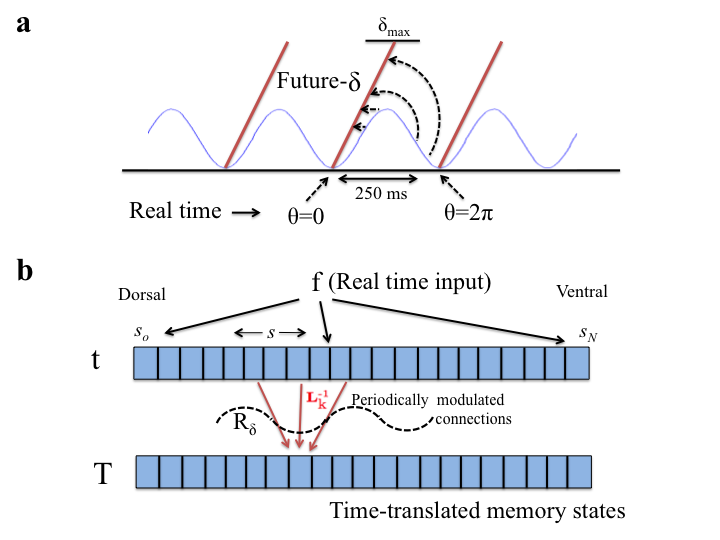
Figure 1: a. Theta oscillations of 4-8 Hz are observed in the voltage recorded from the hippocampus. Hypothesis: Within a theta cycle, a timeline of future translations of magnitude $\delta$ is constructed. b. Two layer network with theta-modulated connections. The $\mathbf{t}$ layer receives external input $\mathbf{f}{}$ in real time and encodes its Laplace transform. The Laplace transform is inverted via a synaptic operator $\mathbf{L}^{\textrm{\scriptsize{-1}}}_{\textrm{k}}$ to yield an estimate of the function $\mathbf{f}{}$ on the $\mathbf{T}$ layer nodes. By periodically manipulating the weights in $\mathbf{L}^{\textrm{\scriptsize{-1}}}_{\textrm{k}}$, the memory state represented in $\mathbf{T}$ layer can be translated to represent its future states.

Motivated by the spatial and temporal memory represented in the hippocampus, we hypothesize that the translation operation required to anticipate the events at a distant future engages this part of the brain Hasselmo et al. (2007); Schacter et al. (2007). We hypothesize that theta oscillations, a well-characterized rhythm of 4-8 Hz in the local field potential observed in the hippocampus may be responsible for the translation operation. In particular, we hypothesize that sequential translations of different magnitudes take place at different phases within a cycle of theta oscillation, such that a timeline of anticipated future events (or equivalently a spaceline of anticipated events at distant locations) is swept out in a single cycle (fig. 1a).

Theta oscillations are prominently observed during periods of navigation Vanderwolf (1969). Critically, there is a systematic relationship between the animal’s position within a neuron’s place field and the phase of the theta oscillation at which that neuron fires O’Keefe and Recce (1993), known as phase precession. This suggests that the phase of firing of the place cells conveys information about the anticipated future location of the animal. This provides a strong motivation for our hypothesis that the phase of theta oscillation would be linked to the translation operation.

I.1 Overview

This paper develops a computational mechanism for the translation operation of a spatial/temporal memory representation constructed from a two-layer neural network model Shankar and Howard (2012), and links it to theta oscillations by imposing certain constraints based on some neurophysiological observations and some physical principles we expect the brain to satisfy. Since the focus here is to understand the computational mechanism of a higher level cognitive phenomena, the imposed constraints and the resulting derivation should be viewed at a phenomenological level, and not as emerging from biophysically detailed neural interactions.

Computationally, we assume that the memory representation is constructed by a two-layer network (fig. 1b) where the first layer encodes the Laplace transform of externally observed stimuli in real time, and the second layer approximately inverts the Laplace transform to represent a fuzzy estimate of the actual stimulus history Shankar and Howard (2012). With access to instantaneous velocity of motion, this two layer network representing temporal memory can be straightforwardly generalized to represent one-dimensional spatial memory Howard et al. (2014). Hence in the context of this two layer network, time-translation of the temporal memory representation can be considered mathematically equivalent to space-translation of the spatial memory representation.

Based on a simple, yet powerful, mathematical observation that translation operation can be performed in the Laplace domain as an instantaneous point-wise product, we propose that the translation operation is achieved by modulating the connection weights between the two layers within each theta cycle (fig. 1b). The translated representations can then be used to predict events at distant future and remote locations. In constructing the translation operation, we impose two physical principles we expect the brain to satisfy. The first principle is scale-invariance, the requirement that all scales (temporal or spatial) represented in the memory are treated equally in implementing the translation. The second principle is coherence, the requirement that at any moment all nodes forming the memory representation are in sync, translated by the same amount.

Further, to implement the computational mechanism of translation as a neural mechanism, we impose certain phenomenological constraints based on neurophysiological observations. First, there exists a dorsoventral axis in the hippocampus of a rat’s brain, and the size of place fields increase systematically from the dorsal to the ventral end Jung et al. (1994); Kjelstrup et al. (2008). In light of this observation, we hypothesize that the nodes representing different temporal and spatial scales of memory are ordered along the dorsoventral axis. Second, the phase of theta oscillation is not uniform along the dorsoventral axis; phase advances from the dorsal to the ventral end like a traveling wave Lubenov and Siapas (2009); Patel et al. (2012) with a phase difference of about $\pi$ from one end to the other. Third, the synaptic weights change as a function of phase of the theta oscillation throughout the hippocampus Wyble et al. (2000); Schall et al. (2008). In light of this observation, we hypothesize that the change in the connection strengths between the two layers required to implement the translation operation depend only on the local phase of the theta oscillation at any node (neuron).

In section II, we impose the above mentioned physical principles and phenomenological constraints to derive quantitative relationships for the distribution of scales of the nodes representing the memory and the theta-phase dependence of the translation operation. This yields specific forms of phase-precession in the nodes representing the memory as well as the nodes representing future prediction. Section III compares these forms to neurophysiological phase precession observed in the hippocampus and ventral striatum. Section III also makes explicit neurophysiological predictions that could verify our hypothesis that theta oscillations implement the translation operation to construct a timeline of future predictions.

II Mathematical model

In this section we start with a basic overview of the two layer memory model and summarize the relevant details from previous work Shankar and Howard (2012, 2013); Howard et al. (2014) to serve as a background. Following that, we derive the equations that allow the memory nodes to be coherently time-translated to various future moments in synchrony with the theta oscillations. Finally we derive the predictions generated for various future moments from the time-translated memory states.

II.1 Theoretical background

The memory model is implemented as a two-layer feedforward network (fig. 1b) where the $\mathbf{t}$ layer holds the Laplace transform of the recent past and the $\mathbf{T}$ layer reconstructs a temporally fuzzy estimate of past events Shankar and Howard (2012, 2013). Let the stimulus at any time $\tau$ be denoted as $\mathbf{f}{}(\tau)$. The nodes in the $\mathbf{t}$ layer are leaky integrators parametrized by their decay rate $s$, and are all independently activated by the stimulus. The nodes are assumed to be arranged w.r.t. their $s$ values. The nodes in the $\mathbf{T}$ layer are in one to one correspondence with the nodes in the $\mathbf{t}$ layer and hence can also be parametrized by the same $s$. The feedforward connections from the $\mathbf{t}$ layer into the $\mathbf{T}$ layer are prescribed to satisfy certain mathematical properties which are described below. The activity of the two layers is given by

$$\frac{d}{d\tau}\mathbf{t}(\tau,s) = -s\mathbf{t}(\tau,s)+\mathbf{f}{}(\tau)$$ (1)

$$\mathbf{T}(\tau,s) = [\mathbf{L}^{\textrm{\scriptsize{-1}}}_{\textrm{k}}]\,\mathbf{t}(\tau,s)$$ (2)

By integrating eq. 1, note that the $\mathbf{t}$ layer encodes the Laplace transform of the entire past of the stimulus function leading up to the present. The $s$ values distributed over the $\mathbf{t}$ layer represent the (real) Laplace domain variable. The fixed connections between the $\mathbf{t}$ layer and $\mathbf{T}$ layer denoted by the operator $\mathbf{L}^{\textrm{\scriptsize{-1}}}_{\textrm{k}}$ (in eq. 2), is constructed to reflect an approximation to inverse Laplace transform. In effect, the Laplace transformed stimulus history which is distributed over the $\mathbf{t}$ layer nodes is inverted by $\mathbf{L}^{\textrm{\scriptsize{-1}}}_{\textrm{k}}$ such that a fuzzy (or coarse grained) estimate of the actual stimulus value from various past moments is represented along the different $\mathbf{T}$ layer nodes.

More precisely, treating the $s$ values nodes as continuous, the $\mathbf{L}^{\textrm{\scriptsize{-1}}}_{\textrm{k}}$ operator can be succinctly expressed as

$$\mathbf{T}(\tau,s)=\frac{(-1)^{k}}{k!}s^{k+1}\mathbf{t}^{(k)}(\tau,s)\equiv[\mathbf{L}^{\textrm{\scriptsize{-1}}}_{\textrm{k}}]\,\mathbf{t}(\tau,s)$$ (3)

Here $\mathbf{t}^{(k)}(\tau,s)$ corresponds to the $k$-th derivative of $\mathbf{t}(\tau,s)$ w.r.t. $s$. It can be proven that $\mathbf{L}^{\textrm{\scriptsize{-1}}}_{\textrm{k}}$ operator executes an approximation to the inverse Laplace transformation and the approximation grows more and more accurate for larger and larger values of $k$ Post (1930). Further details of $\mathbf{L}^{\textrm{\scriptsize{-1}}}_{\textrm{k}}$ depends on the $s$ values chosen for the nodes Shankar and Howard (2013), but these details are not relevant for this paper as the $s$ values of neighboring nodes are assumed to be close enough that the analytic expression for $\mathbf{L}^{\textrm{\scriptsize{-1}}}_{\textrm{k}}$ given by eq. 3 would be accurate.

To emphasize the properties of this memory representation, consider the stimulus $\mathbf{f}{}(\tau)$ to be a Dirac delta function at $\tau=0$. From eq. 1 and 3, the $\mathbf{T}$ layer activity following the stimulus presentation ($\tau>0$) turns out to be

$$\mathbf{T}(\tau,s)=\frac{s}{k!}\left[s\tau\right]^{k}e^{-\left[s\tau\right]}$$ (4)

Note that nodes with different $s$ values in the $\mathbf{T}$ layer peak in activity after different delays following the stimulus; hence the $\mathbf{T}$ layer nodes behave like time cells. In particular, a node with a given $s$ peaks in activity at a time $\tau=k/s$ following the stimulus. Moreover, viewing the activity of any node as a distribution around its appropriate peak-time ($k/s$), we see that the shape of this distribution is exactly the same for all nodes to the extent $\tau$ is rescaled to align the peaks of all the nodes. In other words, the activity of different nodes of the $\mathbf{T}$ layer represent a fuzzy estimate of the past information from different timescales and the fuzziness associated with them is directly proportional to the timescale they represent, while maintaining the exact same shape of fuzziness. For this reason, the $\mathbf{T}$ layer represents the past information in a scale-invariant fashion.

This two-layer memory architecture is also amenable to represent one-dimensional spatial memory analogous to the representation of temporal memory in the $\mathbf{T}$ layer Howard et al. (2014). If the stimulus $\mathbf{f}{}$ is interpreted as a landmark encountered at a particular location in a one-dimensional spatial arena, then the $\mathbf{t}$ layer nodes can be made to represent the Laplace transform of the landmark treated as a spatial function with respect to the current location. By modifying eq. 1 to

$$\frac{d}{d\tau}\mathbf{t}(\tau,s)=v\left[-s\mathbf{t}(\tau,s)+\mathbf{f}{}(\tau)\right],$$ (5)

where $v$ is the velocity of motion, the temporal dependence of the $\mathbf{t}$ layer activity can be converted to spatial dependence. By employing the $\mathbf{L}^{\textrm{\scriptsize{-1}}}_{\textrm{k}}$ operator on this modified $\mathbf{t}$ layer activity (eq. 5), it is straightforward to construct a layer of nodes (analogous to $\mathbf{T}$) that exhibit peak activity at different distances from the landmark. Thus the two-layer memory architecture can be trivially extended to yield place-cells in one dimension.

In what follows, rather than referring to translation operations separately on spatial and temporal memory, we shall simply consider time-translations with an implicit understanding that all the results derived can be trivially extended to 1-d spatial memory representations.

II.2 Time-translating the Memory state

The two-layer architecture naturally lends itself for time-translations of the memory state in the $\mathbf{T}$ layer, which we shall later exploit to construct a timeline of future predictions. The basic idea is that if the current state of memory represented in the $\mathbf{T}$ layer is used to anticipate the present (via some prediction mechanism), then a time-translated state of $\mathbf{T}$ layer can be used to predict events that will occur at a distant future via the same prediction mechanism. Time-translation means to mimic the $\mathbf{T}$ layer activity at a distant future based on its current state. Ideally translation should be non-destructive, not overwriting the current activity in the $\mathbf{t}$ layer.

Let $\delta$ be the amount by which we intend to time-translate the state of $\mathbf{T}$ layer. So, at any time $\tau$, the aim is to access $\mathbf{T}(\tau+\delta,s)$ while still preserving the current $\mathbf{t}$ layer activity, $\mathbf{t}(\tau,s)$. This is can be easily achieved because the $\mathbf{t}$ layer represents the stimulus history in the Laplace domain. Noting that the Laplace transform of a $\delta$-translated function is simply the product of $e^{-s\delta}$ and the Laplace transform of the un-translated function, we see that

$$\mathbf{t}(\tau+\delta,s) = e^{-s\delta}\mathbf{t}(\tau,s)$$ (6)

Now noting that $\mathbf{T}(\tau+\delta,s)$ can be obtained by employing the $\mathbf{L}^{\textrm{\scriptsize{-1}}}_{\textrm{k}}$ operator on $\mathbf{t}(\tau+\delta,s)$ analogous to eq. 3, we obtain the $\delta$-translated $\mathbf{T}$ activity as

$$\mathbf{T}_{\delta}(\tau,s)\equiv\mathbf{T}(\tau+\delta,s) = [\mathbf{L}^{\textrm{\scriptsize{-1}}}_{\textrm{k}}]\,\mathbf{t}(\tau+\delta,s)$$ (7)

$$= \left[\mathbf{L}^{\textrm{\scriptsize{-1}}}_{\textrm{k}}\cdot\mathbf{R}_{\delta}\right]\,\mathbf{t}(\tau,s)$$

where $\mathbf{R}_{\delta}$ is just a diagonal operator whose rows and columns are indexed by $s$ and the diagonal entries are $e^{-s\delta}$. The $\delta$-translated activity of the $\mathbf{T}$ layer is now subscripted by $\delta$ as $\mathbf{T}_{\delta}$ so as to distinguish it from the un-translated $\mathbf{T}$ layer activity given by eq. 3 without a subscript. In this notation the un-translated state $\mathbf{T}(\tau,s)$ from eq. 3 can be expressed as $\mathbf{T}_{0}(\tau,s)$. The time-translated $\mathbf{T}$ activity can be obtained from the current $\mathbf{t}$ layer activity if the connection weights between the two layers given by $\mathbf{L}^{\textrm{\scriptsize{-1}}}_{\textrm{k}}$ is modulated by $\mathbf{R}_{\delta}$. This computational mechanism of time-translation can be implemented as a neural mechanism in the brain, by imposing certain phenomenological constraints and physical principles.

Observation 1: Anatomically, along the dorsoventral axis of the hippocampus, the width of place fields systematically increases from the dorsal end to the ventral end Jung et al. (1994); Kjelstrup et al. (2008). Fig. 2 schematically illustrates this observation by identifying the $s$-axis of the two-layer memory architecture with the dorso-ventral axis of the hippocampus, such that the scales represented by the nodes are monotonically arranged. Let there be $N+1$ nodes with monotonically decreasing $s$ values given by $s_{o}$, $s_{1}$, …$s_{N}$.

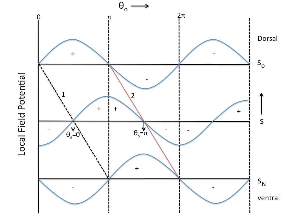
Figure 2: Traveling theta wave along the $s$ axis. The x-axis is real time. Each point along the dorsoventral axis corresponds to a different value of $s_{n}$. The curvy blue lines show the theta oscillation for several different values of $s$. Lines 1 and 2 connect the positions where the local phases $\theta_{s}$ are 0 and $\pi$ respectively.

Observation 2: The phase of the theta oscillations along the axis is non-uniform, representing a traveling wave from the dorsal to ventral part of the hippocampus with a net phase shift of $\pi$ Lubenov and Siapas (2009); Patel et al. (2012). The oscillations in fig. 2 symbolize the local field potentials at different locations of the $s$-axis. The local phase of the oscillation at any position on the $s$-axis is denoted by $\theta_{s}$, which ranges from $-\pi$ to $+\pi$ by convention. However, as a reference we denote the phase at the top (dorsal) end as $\theta_{o}$ ranging from $0$ to $2\pi$, with the understanding that the range $(\pi,2\pi)$ is mapped on to $(-\pi,0)$. The $x$-axis in fig. 2 is time within a theta oscillation labeled by the phase $\theta_{o}$.

In this convention, the value of $\theta_{s}$ discontinuously jumps from $+\pi$ to $-\pi$ as we move from one cycle of oscillation to the next. In fig. 2, the diagonal (solid-red) line labeled ‘2’ denotes all the points where this discontinuous jump happens. The diagonal (dashed) line labeled ‘1’ denotes all the points where $\theta_{s}=0$. It is straightforward to infer the relationship between the phase at any two values of $s$. Taking the nodes to be uniformly spaced anatomically, the local phase $\theta_{s}$ of the $n$-th node is related to $\theta_{o}$ (for $0<\theta_{s}<\pi$) by

$$\theta_{s}/\pi=\theta_{o}/\pi-n/N.$$ (8)

Observation 3: Synaptic weights in the hippocampus are modulated periodically in synchrony with the phase of theta oscillation Wyble et al. (2000); Schall et al. (2008). Based on this observation, we impose the constraint that the connection strengths between the $\mathbf{t}$ and $\mathbf{T}$ layers at a particular value of $s$ depend only on the local phase of the theta oscillations. Thus the diagonal entries in the $\mathbf{R}_{\delta}$ operator should only depend on $\theta_{s}$. We take these entries to be of the form $\exp{(-\Phi_{s}(\theta_{s}))}$, where $\Phi_{s}$ is any continuous function of $\theta_{s}\in(-\pi,+\pi)$. Heuristically, at any moment within a theta cycle, a $\mathbf{T}$ node with a given $s$ value will be roughly translated by an amount $\delta=\Phi_{s}(\theta_{s})/s$.

Principle 1: Preserve Scale-Invariance

Scale-invariance is an extremely adaptive property for a memory to have; in many cases biological memories seem to exhibit scale-invariance Balsam and Gallistel (2009). As the untranslated $\mathbf{T}$ layer activity already exhibits scale-invariance, we impose the constraint that the time-translated states of $\mathbf{T}$ should also exhibit scale-invariance. This consideration requires the behavior of every node to follow the same pattern with respect to their local theta phase. This amounts to choosing the functions $\Phi_{s}$ to be the same for all $s$, which we shall refer to as $\Phi$.

Principle 2: Coherence in translation

Since the time-translated memory state is going to be used to make predictions for various moments in the distant future, it would be preferable if all the nodes are time-translated by the same amount at any moment within a theta cycle. If not, different nodes would contribute to predictions for different future moments leading to noise in the prediction. However, such a requirement of global coherence cannot be imposed consistently along with the principle 1 of preserving scale-invariance. But in the light of prior work Hasselmo et al. (2002); Hasselmo (2012) which suggest that retrieval of memory or prediction happens only in one half of the theta cycle, we impose the requirement of coherence only to those nodes that are all in the positive half of the cycle at any moment. That is, $\delta=\Phi(\theta_{s})/s$ is a constant along any vertical line in the region bounded between the diagonal lines 1 and 2 shown in fig. 2. Hence for all nodes with $0<\theta_{s}<\pi$, we require

$$\Delta\left(\Phi\left(\theta_{s}\right)/s\right)=\Delta\left(\Phi\left(\theta_{o}-\pi n/N\right)/s_{n}\right)=0.$$ (9)

For coherence as expressed in eq. 9 to hold at all values of $\theta_{o}$ between 0 and $2\pi$, $\Phi(\theta_{s})$ must be an exponential function so that $\theta_{o}$ can be functionally decoupled from $n$; consequently $s_{n}$ should also have an exponential dependence on $n$. So the general solution to eq. 9 when $0<\theta_{s}<\pi$ can be written as

$$\Phi(\theta_{s}) = \Phi_{o}\exp{[b\theta_{s}]}$$ (10)

$$s_{n} = s_{o}(1+c)^{-n}$$ (11)

where $c$ is a positive number. In this paper, we shall take $c\ll 1$, so that the analytic approximation for the $\mathbf{L}^{\textrm{\scriptsize{-1}}}_{\textrm{k}}$ operator given in terms of the $k$-th derivative along the $s$ axis in eq. 3 is valid.

Thus the requirement of coherence in time-translation implies that the $s$ values of the nodes—the timescales represented by the nodes—are spaced out exponentially, which can be referred to as a Weber-Fechner scale, a commonly used terminology in cognitive science. Remarkably, this result strongly resonates with a requirement of the exact same scaling when the predictive information contained in the memory system is maximized in response to long-range correlated signals Shankar and Howard (2013). This feature allows this memory system to represent scale-invariantly coarse grained past information from timescales exponentially related to the number of nodes.

The maximum value attained by the function $\Phi(\theta_{s})$ is at $\theta_{s}=\pi$, and the maximum value is $\Phi_{\textnormal{max}}=\Phi_{o}\exp{[b\pi]}$, such that $\Phi_{\textnormal{max}}/\Phi_{o}=s_{o}/s_{N}$ and $b=(1/\pi)\log{(\Phi_{\textnormal{max}}/\Phi_{o})}$. To ensure continuity around $\theta_{s}=0$, we take the eq. 10 to hold true even for $\theta_{s}\in(-\pi,0)$. However, since notationally $\theta_{s}$ makes a jump from $+\pi$ to $-\pi$, $\Phi(\theta_{s})$ would exhibit a discontinuity at the diagonal line 2 in fig. 2 from $\Phi_{\textnormal{max}}$ (corresponding to $\theta_{s}=\pi$) to $\Phi_{\textnormal{min}}=\Phi_{o}^{2}/\Phi_{\textnormal{max}}$ (corresponding to $\theta_{s}=-\pi$).

Given these considerations, at any instant within a theta cycle, referenced by the phase $\theta_{o}$, the amount $\delta$ by which the memory state is time-translated can be derived from eq. 8 and 10 as

$$\delta(\theta_{o})=(\Phi_{o}/s_{o})\exp{[b\theta_{o}]}.$$ (12)

Analogous to having the past represented on a Weber-Fechner scale, the translation distance $\delta$ into the future also falls on a Weber-Fechner scale as the theta phase is swept from 0 to $2\pi$. In other words, the amount of time spent within a theta cycle for larger translations is exponentially smaller.

To emphasize the properties of the time-translated $\mathbf{T}$ state, consider the stimulus to be a Dirac delta function at $\tau=0$. From eq. 7, we can express the $\mathbf{T}$ layer activity analogous to eq. 4.

$$\mathbf{T}_{\delta}(\tau,s)\simeq\frac{s}{k!}\left[s\tau+\Phi\left(\theta_{s}\right)\right]^{k}e^{-\left[s\tau+\Phi\left(\theta_{s}\right)\right]}$$ (13)

Notice that eqs. 8 and 12 specify a unique relationship between $\delta$ and $\theta_{s}$ for any given $s$. The r.h.s. above is expressed in terms of $\theta_{s}$ rather than $\delta$ so as to shed light on the phenomenon of phase precession.

Since $\mathbf{T}_{\delta}(\tau,s)$ depends on both $\tau$ and $\theta_{s}$ only via the sum $[s\tau+\Phi\left(\theta_{s}\right)]$, a given node will show identical activity for various combinations of $\tau$ and $\theta_{s}$. For instance, a node would achieve its peak activity when $\tau$ is significantly smaller than its timescale $(k/s)$ only when $\Phi(\theta_{s})$ is large—meaning $\theta_{s}\simeq+\pi$. And as $\tau$ increases towards the timescale of the node, the peak activity gradually shifts to earlier phases all the way to $\theta_{s}\simeq-\pi$. An important consequence of imposing principle 1 is that the relationship between $\theta_{s}$ and $\tau$ on any iso-activity contour is scale-invariant. That is, every node behaves similarly when $\tau$ is rescaled by the timescale of the node. We shall further pursue the analogy of this phenomenon of phase precession with neurophysiological findings in the next section (fig. 4).

II.3 Timeline of Future Prediction

At any moment, $\mathbf{T}_{\delta}$ (eq. 13) can be used to predict the stimuli expected at a future moment. Consequently, as $\delta$ is swept through within a theta cycle, a timeline of future predictions can be simulated in an orderly fashion, such that predictions for closer events occur at earlier phases (smaller $\theta_{o}$) and predictions of distant events occur at later phases. In order to predict from a time-translated state $\mathbf{T}_{\delta}$, we need a prediction mechanism. For our purposes, we consider here a very simple form of learning and prediction, Hebbian association. In this view, an event is learned (or an association formed in long term memory) by increasing the connection strengths between the neurons representing the currently-experienced stimulus and the neurons representing the recent past events ($\mathbf{T}_{0}$). Because the $\mathbf{T}$ layer activity contains temporal information about the preceding stimuli, simple associations between $\mathbf{T}_{0}$ and the current stimulus are sufficient to encode and express well-timed predictions Shankar and Howard (2012). In particular, the term Hebbian implies that the change in each connection strength is proportional to the product of pre-synaptic activity—in this case the activity of the corresponding node in the $\mathbf{T}$ layer—and post-synaptic activity corresponding to the current stimulus. Given that the associations are learned in this way, we define the prediction of a particular stimulus to be the scalar product of its association strengths with the current state of $\mathbf{T}$. In this way, the scalar product of association strengths and a translated state $\mathbf{T}_{\delta}$ can be understood as the future prediction of that stimulus.

Consider the thought experiment where a conditioned stimulus cs is consistently followed by another stimulus, a or b, after a time $\tau_{o}$. Later when cs is repeated (at a time $\tau=0$), the subsequent activity in the $\mathbf{T}$ nodes can be used to generate predictions for the future occurrence of a or b. The connections to the node corresponding to a will be incremented by the state of $\mathbf{T}_{0}$ when a is presented; the connections to the node corresponding to b will be incremented by the state of $\mathbf{T}_{0}$ when b is presented. In the context of Hebbian learning, the prediction for the stimulus at a future time as a function of $\tau$ and $\tau_{o}$ is obtained as the sum of $\mathbf{T}_{\delta}$ activity of each node multiplied by the learned association strength ($\mathbf{T}_{0}$):

$$\mathbf{p}_{\delta}(\tau,\tau_{o})=\sum_{n=\ell}^{N}\mathbf{T}_{\delta}\left(\tau,s_{n}\right)\ \mathbf{T}_{0}\left(\tau_{o},s_{n}\right)/s_{n}^{w}.$$ (14)

The factor $s_{n}^{w}$ (for any $w$) allows for differential association strengths for the different $s$ nodes, while still preserving the scale invariance property. Since $\delta$ and $\theta_{o}$ are monotonically related (eq. 12), the prediction $\mathbf{p}_{\delta}$ for various future moments happens at various phases of a theta cycle.

Recall that all the nodes in the $\mathbf{T}$ layer are coherently time-translated only in the positive half of the theta cycle. Hence for computing future predictions based on a time-translated state $\mathbf{T}_{\delta}$, only coherent nodes should contribute. In fig. 2, the region to the right of diagonal line 2 does not contribute to the prediction. The lower limit $\ell$ in the summation over the nodes given in eq. 14 is the position of the diagonal line 2 in fig. 2 marking the position of discontinuity where $\theta_{s}$ jumps from $+\pi$ to $-\pi$.

In the limit when $c\rightarrow 0$, the $s$ values of neighboring nodes are very close and the summation can be approximated by an integral. Defining $x=s\tau_{o}$ and $y=\tau/\tau_{o}$ and $v=\delta/\tau_{o}$, the above summation can be rewritten as

$$\mathbf{p}_{\delta}(\tau,\tau_{o})\simeq\frac{\tau_{o}^{w-2}}{k!^{2}}\int_{x_{min}}^{x_{u}}x^{2k+1-w}(y+v)^{k}e^{-x(1+y+v)}\,dx$$ (15)

Here $x_{min}=s_{N}\tau_{o}$, and $x_{u}=s_{o}\tau_{o}$ for $0<\theta_{o}<\pi$ and $x_{u}=\Phi_{max}\tau_{o}/\delta$ for $\pi<\theta_{o}<2\pi$. The integral can be evaluated in terms of lower incomplete gamma functions to be

$$\mathbf{p}_{\delta} (\tau,\tau_{o})\simeq\frac{\tau_{o}^{w-2}}{k!^{2}}\frac{\left[(\tau+\delta)/\tau_{o}\right]^{k}}{[1+(\tau+\delta)/\tau_{o}]^{C}}\,\times$$ (16)

$$\left(\Gamma\left[C,(\tau_{o}+\tau+\delta)U\right]-\Gamma\left[C,(\tau_{o}+\tau+\delta)s_{N}\right]\right),$$

where $C=2k+2-w$ and $\Gamma[.,.]$ is the lower incomplete gamma function. For $\theta_{o}<\pi$ (i.e., when $\delta<\Phi_{\textnormal{max}}/s_{o}$), $U=s_{o}$ and for $\theta_{o}>\pi$ (i.e., when $\delta>\Phi_{\textnormal{max}}/s_{o}$), $U=\Phi_{\textnormal{max}}/\delta$.

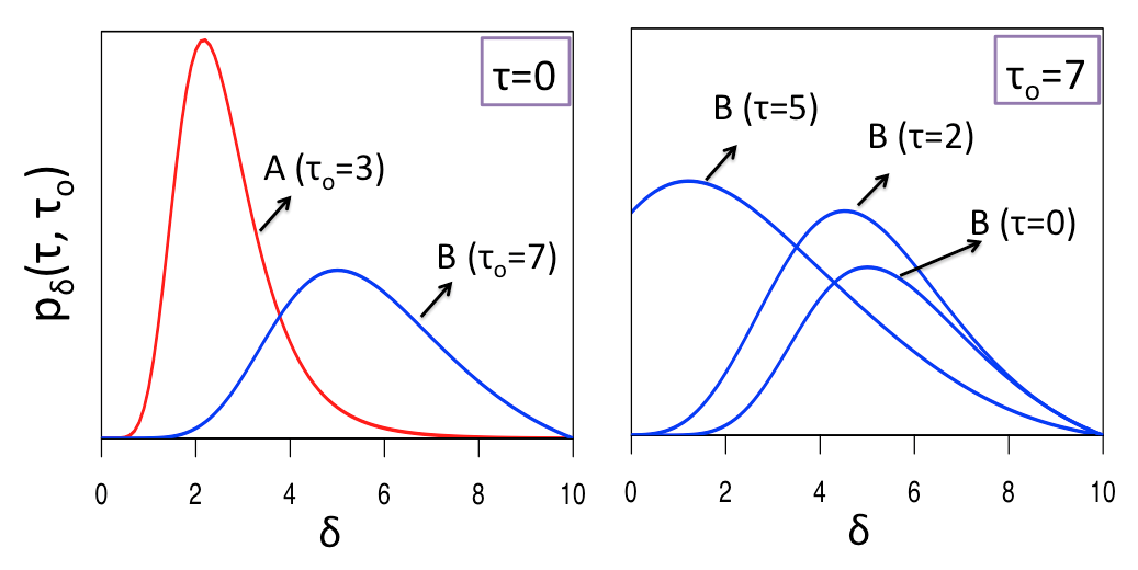
Figure 3: Future timeline. Eq. 16 is plotted as a function of $\delta$. During training, the cs was presented at $\tau_{o}=3$ before a and $\tau_{o}=7$ before b. Left: Immediately after presentation of the cs, the predictions for a and b are ordered on the $\delta$ axis. Note that the prediction for b approximates a rescaled version of that for a. Right: The prediction for b is shown for varying times after presentation of cs. With the passage of time, the prediction of b becomes stronger and more imminent. In this figure, $\Phi_{\textnormal{max}}=10$, $\Phi_{o}=1$, $k=10$, $s_{o}=10$, $s_{N}=1$, and $w=1$.

Figure 3 provides a graphical representation of some key properties of eq. 16. The figure assumes that the cs is followed by a after $\tau_{o}=3$ and followed by b after $\tau_{o}=7$. The left panel shows the predictions for both a and b as a function of $\delta$ immediately after presentation of cs. The prediction for a appears at smaller $\delta$ and with a higher peak than the prediction for b. The value of $w$ affects the relative sizes of the peaks. The right panel shows how the prediction for b changes with the passage of time after presentation of the cs. As $\tau$ increases from zero and the cs recedes into the past, the prediction of b peaks at smaller values of $\delta$, corresponding to more imminent future times. In particular when $\tau_{o}$ is much smaller than the largest (and larger than the smallest) timescale represented by the nodes, then the shape of $\mathbf{p}_{\delta}$ remains the same when $\delta$ and $\tau$ are rescaled by $\tau_{o}$. Under these conditions, the timeline of future predictions generated by $\mathbf{p}_{\delta}$ is scale-invariant.

Since $\delta$ is in one-to-one relationship with $\theta_{o}$, as a predicted stimulus becomes more imminent, the activity corresponding to that predicted stimulus should peak at earlier and earlier phases. Hence a timeline of future predictions can be constructed from $\mathbf{p}_{\delta}$ as the phase $\theta_{o}$ is swept from $0$ to $2\pi$. Moreover the cells representing $\mathbf{p}_{\delta}$ should show phase precession with respect to $\theta_{o}$. Unlike cells representing $\mathbf{T}_{\delta}$, which depend directly on their local theta phase, $\theta_{s}$, the phase precession of cells representing $\mathbf{p}_{\delta}$ should depend on the reference phase $\theta_{o}$ at the dorsal end of the $s$-axis. We shall further connect this neurophysiology in the next section (fig. 6).

III Comparisons with Neurophysiology

The mathematical development focused on two entities $\mathbf{T}_{\delta}$ and $\mathbf{p}_{\delta}$ that change their value based on the theta phase (eqs. 13 and 16). In order to compare these to neurophysiology, we need to have some hypothesis linking them to the activity of neurons from specific brain regions. We emphasize that although the development in the preceding section was done with respect to time, all of the results generalize to one-dimensional position as well (eq. 5, Howard et al. (2014)). The overwhelming majority of evidence for phase precession comes from studies of place cells (but see Pastalkova et al. (2008)). Here we compare the properties of $\mathbf{T}_{\delta}$ to phase precession in hippocampal neurons and the properties of $\mathbf{p}_{\delta}$ to a study showing phase precession in ventral striatum van der Meer and Redish (2011).

Due to various analytic approximations, the activity of nodes in the $\mathbf{T}$ layer as well as the activity of the nodes representing future prediction (eqs. 13 and 16) are expressed as smooth functions of time and theta phase. However, neurophysiologically, discrete spikes (action potentials) are observed. In order to facilitate comparison of the model to neurophysiology, we adopt a simple stochastic spike-generating method. In this simplistic approach, the activity of the nodes given by eqs. 13 and 16 are taken to be proportional to the instantaneous probability for generating a spike. The probability of generating a spike at any instant is taken to be the instantaneous activity divided by the maximum activity achieved by the node if the activity is greater than 60% of the maximum activity. In addition, we add spontaneous stochastic spikes at any moment with a probability of 0.05. For all of the figures in this section, the parameters of the model are set as $k=10$, $\Phi_{\textnormal{max}}=10$, $w=2$, $\Phi_{o}=1$, $s_{N}=1$, $s_{o}=10$.

This relatively coarse level of realism in spike generation from the analytic expressions is probably appropriate to the resolution of the experimental data. There are some experimental challenges associated with exactly evaluating the model. First, theta phase has to be estimated from a noisy signal. Second, phase precession results are typically shown as averaged across many trials. It is not necessarily the case that the average is representative of an individual trial (although this is the case at least for phase-precessing cells in medial entorhinal cortex Reifenstein et al. (2012)). Finally, the overwhelming majority of phase precession experiments utilize extracellular methods, which cannot perfectly identify spikes from individual neurons.

III.1 Hippocampal phase precession

a		b

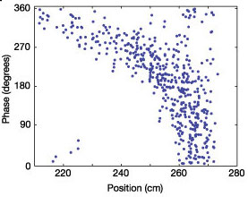
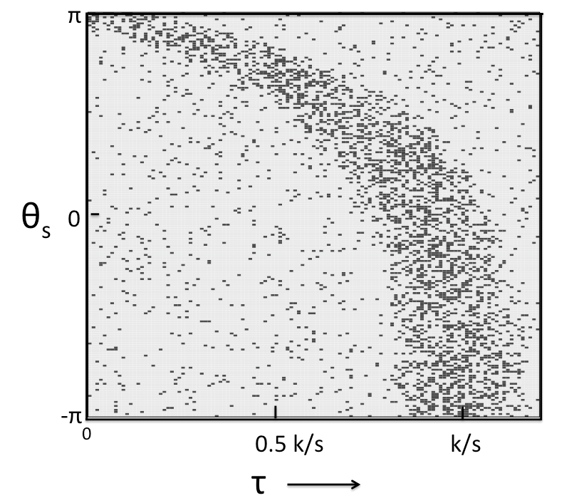
Figure 4: a. Neurophysiological data showing phase precession. Each spike fired by a place cell is shown as a function of its position along a linear track (x-axis) and the phase of local theta (y-axis). After Mehta, et al., 2002. b. Simulated spikes from a node in the $\mathbf{T}$ layer described by eq. 13 as a function of $\tau$ and local phase $\theta_{s}$. The curvature is a consequence of eq. 10. See text for details.

It is clear from eq. 13 that the activity of nodes in the $\mathbf{T}$ layer depends on both $\theta_{s}$ and $\tau$. Figure 4 shows phase precession data from a representative cell (Fig. 4a, Mehta et al. (2002)) and spikes generated from eq. 13 (Fig. 4b). The model generates a characteristic curvature for phase precession, a consequence of the exponential form of the function $\Phi$ (eq. 10). The example cell chosen in fig. 4 shows roughly the same form of curvature as that generated by the model. While it should be noted that there is some variability across cells, careful analyses have led computational neuroscientists to conclude that the canonical form of phase precession resembles this representative cell. For instance, a detailed study of hundreds of phase-precessing neurons Yamaguchi et al. (2002) constructed averaged phase-precession plots using a variety of methods and found a distinct curvature that qualitatively resembles this neuron. Because of the analogy between time and one-dimensional position (eq. 5), the model yields the same pattern of phase precession for time cells and place cells.

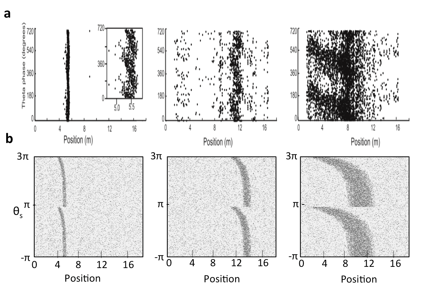
Figure 5: Place cells along the dorsoventral axis of the hippocampus have place fields that increase in size. a. The three panels show the activity of place cells recorded at the dorsal, intermediate and ventral segments of the hippocampus, when a rat runs along an 18 m track. After Kjelstrup, et al., (2008). Each spike the cell fired is shown as a function of position and the local theta phase at the cell’s location when it fires (recall that theta phase is not constant across the dorsoventral axis). Regardless of the width of the place field, neurons at all locations along the dorsoventral axis phase precess through the same range of local theta phases. b. According to the model, phase precession extends over the same range of values of local theta $\theta_{s}$ regardless of the value of $s$, which sets the scale for a particular node. As a consequence, cells with different values of $s$ show time/place fields of different size but phase precess over the same range of local theta. For the three figures, $s$ values of the nodes are set to $.1$, $.22$, and $.7$ respectively, and they are assumed to respond to landmarks at location $4$, $11$, and $3$ meters respectively from one end of the track.

The $\mathbf{T}$ layer activity represented in fig. 4a is scale-invariant; note that the $x$-axis is expressed in units of the scale of the node ($k/s$). It is known that the spatial scale of place fields changes systematically along the dorsoventral axis of the hippocampus. Place cells in the dorsal hippocampus have place fields of the order of a few centimeters whereas place cells at the ventral end have place fields as large as a few meters (fig. 5a) Jung et al. (1994); Kjelstrup et al. (2008). However, all of them show the same pattern of precession with respect to their local theta phase—the phase measured at the same electrode that records a given place cell (fig. 5). Recall that at any given moment, the local phase of theta oscillation depends on the position along the dorsoventral axis Lubenov and Siapas (2009); Patel et al. (2012), denoted as the $s$-axis in the model.

Figure 5a shows the activity of three different place cells in an experiment where rats ran down a long track that extended through open doors connecting three testing rooms Kjelstrup et al. (2008). The landmarks controlling a particular place cell’s firing may have been at a variety of locations along the track. Accordingly, fig. 5b shows the activity of cells generated from the model with different values of $s$ and with landmarks at various locations along the track (described in the caption). From fig. 5 it can be qualitatively noted that phase precession of different cells only depends on the local theta phase and is unaffected by the spatial scale of firing. This observation is perfectly consistent with the model.

III.2 Prediction of distant rewards via phase precession in the ventral striatum

a		b

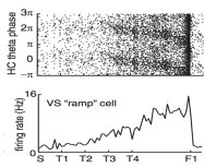
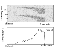
Figure 6: a. A representative ramping cell in the ventral striatum. On each trial the animal started the maze at S, made a series of turns (T1, T2, etc) and received reward at F1 on 75 percent of trials. The total distance between S and F1 is on the order of a few meters. Position along the track is represented linearly on the x-axis for convenience. In the top panel, the spikes are shown as a function of theta phase at the dorsal hippocampus and position. The bottom panel shows the firing rate as a function of position, which is seen to gradually ramp up towards the reward location. b. The activity of prediction node generated by the model is plotted w.r.t. the reference phase $\theta_{o}$ and position in the top panel, and the the average activity within a theta cycle is plotted against position in the bottom panel.

We compare the future predictions generated by the model (eq. 16) to an experiment that recorded simultaneously from the hippocampus and nucleus accumbens, a reward-related structure within the ventral striatum van der Meer and Redish (2011). Here the rat’s task was to learn to make several turns in sequence on a maze to reach two locations where reward was available. Striatal neurons fired over long stretches of the maze, gradually ramping up their firing as a function of distance along the path and terminating at the reward locations (bottom fig. 6a). Many striatal neurons showed robust phase precession relative to the theta phase at the dorsal hippocampus (top fig. 6a). Remarkably, the phase of oscillation in the hippocampus controlled firing in the ventral striatum to a greater extent than the phase recorded from within the ventral striatum. On trials where there was not a reward at the expected location (F1), there was another ramp up to the secondary reward location (F2), accompanied again by phase precession (not shown in fig. 6a).

This experiment corresponds reasonably well to the conditions assumed in the derivation of eq. 16. In this analogy, the start of the trial (start location S) plays the role of the cs and the reward plays the role of the predicted stimulus. However, there is a discrepancy between the methods and the assumptions of the derivation. The ramping cell (fig. 6a) abruptly terminates after the reward is consumed, whereas eq. 16 would gradually decay back towards zero. This is because of the way the experiment was set up–there were never two rewards presented consecutively. As a consequence, having just received a reward strongly predicts that there will not be a reward in the next few moments. In light of this consideration, we force the prediction generated in eq. 16 to be zero beyond the reward location and let the firing be purely stochastic. The top panel of fig. 6b shows the spikes generated by model prediction cells with respect to the reference theta phase $\theta_{o}$, and the bottom panel shows the ramping activity computed as the average firing activity within a complete theta cycle around any moment.

The model correctly captures the qualitative pattern observed in the data. According to the model, the reward starts being predicted at the beginning of the track. Initially, the reward is far in the future, corresponding to a large value of $\delta$. As the animal approaches the location of the reward, the reward moves closer to the present along the $\delta$ axis, reaching zero near the reward location. The ramping activity is a consequence of the exponential mapping between $\delta$ and $\theta_{o}$ in eq. 10. Since the proportion of the theta cycle devoted to large values of $\delta$ is small, the firing rate averaged across all phases will be small, leading to an increase in activity closer to the reward.

III.3 Testable properties of the mathematical model

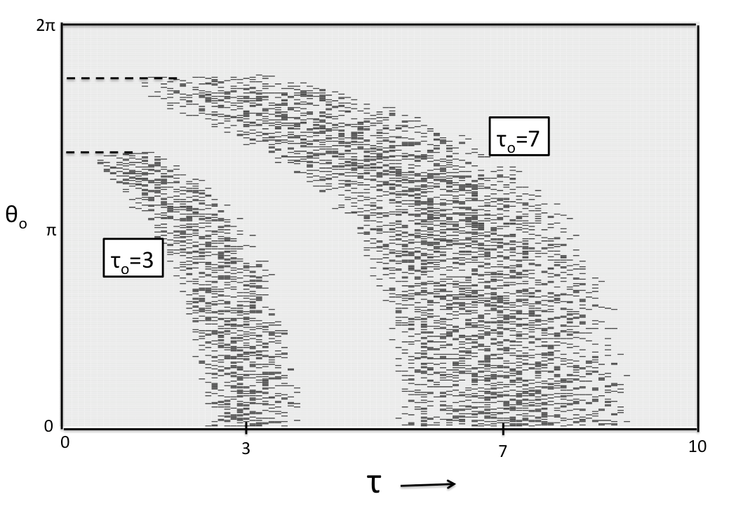
Figure 7: Changing $\tau_{o}$ affects the phase at which prediction cells start firing. At early times, the magnitude of translation required to predict the $\tau_{o}=3$ outcome is smaller than that required to predict the $\tau_{o}=7$ outcome. Consequently, the cell begins to fire at a larger $\theta_{o}$ for $\tau_{o}=7$. Parameter values are the same as the other figures as given in the beginning of this section, except for clarity the background probability of spiking has been set to zero.

Although the model aligns reasonably well with known properties of theta phase precession, there are a number of features of the model that have, to our knowledge, not yet been evaluated. At a coarse level, the correspondence between time and one-dimensional space implies that time cells should exhibit phase precession with the same properties as place cells. While phase precession has been extensively observed and characterized in hippocampal place cells, there is much less evidence for phase precession in hippocampal time cells (but see Pastalkova et al. (2008)).

According to the model, the pattern of phase precession is related to the distribution of $s$ values represented along the dorsoventral axis. While it is known that a range of spatial scales are observed along the dorsoventral axis, their actual distribution is not known. The Weber-Fechner scale of eq. 10 is a strong prediction of the framework developed here. Moreover, since $\Phi_{\textnormal{max}}/\Phi_{o}=s_{o}/s_{N}$, the ratio of the largest to smallest scales represented in the hippocampus places constraints on the form of phase precession. The larger this ratio, the larger will be the value of $b$ in eq. 10, and the curvature in the phase precession plots (as in fig. 4) will only emerge at larger values of the local phase $\theta_{s}$. Neurophysiological observation of this ratio could help evaluate the model.

The form of $\mathbf{p}_{\delta}$ (eq. 16) leads to several distinctive features in the pattern of phase precession of the nodes representing future prediction. It should be possible to observe phase precession for cells that are predicting any stimulus, not just a reward. In addition, the model’s assumption that a timeline of future predictions is aligned with global theta phase has interesting measurable consequences. Let’s reconsider the thought experiment from the previous section (fig. 3), where a stimulus predicts an outcome after a delay $\tau_{o}$. Immediately after the stimulus is presented, the value of $\delta$ at which the prediction peaks is monotonically related to $\tau_{o}$. Since $\delta$ is monotonically related to the reference phase $\theta_{o}$, the prediction cells will begin to fire at later phases when $\tau_{o}$ is large, and as time passes, they will fire at earlier and earlier phases all the way untill $\theta_{o}=0$. In other other words, the entry-phase (at which the firing activity begins) should depend on $\tau_{o}$, the prediction timescale. This is illustrated in fig. 7 with $\tau_{o}=3$ and $\tau_{o}=7$, superimposed on the same graph to make visual comparison easy. The magnitude of the peak activity would in general depend on the value of $\tau_{o}$ except when $w=2$ (as assumed here for visual clarity). Experimentally manipulating the reward times and studying the phase precession of prediction cells could help test this feature.

IV Discussion

This paper presented a neural hypothesis for implementing translations of temporal and 1-d spatial memory states so that future events can be quickly anticipated without destroying the current state of memory. The hypothesis assumes that time cells and place cells observed in the hippocampus represent time or position as a result of a two-layer architecture that encodes and inverts the Laplace transform of external input. It also assumes that sequential translations to progressively more distant points in the future occur within each cycle of theta oscillations. Neurophysiological constraints were imposed as phenomenological rules rather than as emerging from a detailed circuit model. Further, imposing scale-invariance and coherence in translation across memory nodes resulted in Weber-Fechner spacing for the representation of both the past (spacing of $s_{n}$ in the memory nodes) and the future (the relationship between $\delta$ and $\theta_{o}$). Apart from providing cognitive flexibility in accessing a timeline of future predictions at any moment, the computational mechanism described qualitative features of phase precession in the hippocampus and in the ventral striatum. Additionally, we have also pointed out certain distinctive features of the model that can be tested with existing technology.

IV.1 Computational Advantages

The property of the $\mathbf{T}$ layer that different nodes represent the stimulus values from various delays (past moments) is reminiscent of a shift register (or delay-line or synfire chain). However, the two layer network encoding and inverting the Laplace transform of stimulus has several significant computational advantages over a shift register representation.

(i) In the current two-layer network, the spacing of $s$ values of the nodes can be chosen freely. By choosing exponentially spaced $s$-values (Weber-Fechner scaling) as in eq. 10, the $\mathbf{T}$ layer can represent memory from exponentially long timescales compared to a shift register with equal number of nodes, thus making it extremely resource-conserving. Although information from longer timescales is more coarse-grained, it turns out that this coarse-graining is optimal to represent and predict long-range correlated signals Shankar and Howard (2013).

(ii) The memory representation of this two layer network is naturally scale-invariant (eq. 4). To construct a scale-invariant representation from a shift register, the shift register would have to be convolved with a scale-invariant coarse-graining function at each moment, which would be computationally very expensive. Moreover, it turns out that any network that can represent such scale-invariant memory can be identified with linear combinations of multiple such two layer networks Shankar (2015).

(iii) Because translation can be trivially performed when we have access to the Laplace domain, the two layer network enables translations by an amount $\delta$ without sequentially visiting the intermediate states $<\delta$. This can be done by directly changing the connection strengths locally between the two layers as prescribed by diagonal $\mathbf{R}_{\delta}$ operator for any chosen $\delta$. Consequently the physical time taken for the translation can be decoupled from the magnitude of translation. One could imagine a shift register performing a translation operation by an amount $\delta$ either by shifting the values sequentially from one node to the next for $\delta$ time steps or by establishing non-local connections between far away nodes. The latter would make the computation very cumbersome because it would require every node in the register to be connected to every other node (since this should work for any $\delta$), which is in stark contrast with the local connectivity required by our two layer network to perform any translation.

Many previous neurobiological models of phase precession have been proposed Lisman and Jensen (2013); Mehta et al. (2002); Burgess et al. (2007); Hasselmo (2012), and many assume that sequentially activated place cells firing within a theta cycle result from direct connections between those cells Jensen and Lisman (1996), not unlike a synfire chain. Although taking advantage of the Laplace domain in the two layer network to perform translations is not the only possibility, it seems to be computationally powerful compared to the obvious alternatives.

IV.2 Translations without theta oscillations

Although this paper focused on sequential translation within a theta cycle, translation may also be accomplished via other neurophysiological mechanisms. Sharp wave ripple (SRW) events last for about 100 ms and are often accompanied by replay events–sequential firing of place cells corresponding to locations different from the animal’s current location Davidson et al. (2009); Dragoi and Tonegawa (2011); Foster and Wilson (2006); Pfeiffer and Foster (2013); Jadhav et al. (2012). Notably, experimentalists have also observed preplay events during SWRs, sequential activation of place cells that correspond to trajectories that have never been previously traversed, as though the animal is planning a future path Dragoi and Tonegawa (2011); Ólafsdóttir et al. (2015). Because untraversed trajectories could not have been used to learn and build sequential associations between the place cells along the trajectory, the preplay activity could potentially be a result of a translation operation on the overall spatial memory representation.

Sometimes during navigation, a place cell corresponding to a distant goal location gets activated Pfeiffer and Foster (2013), as though a finite distance translation of the memory state has occurred. More interestingly, sometimes a reverse-replay is observed in which place cells are activated in reverse order spreading back from the present location Foster and Wilson (2006). This is suggestive of translation into the past (as if $\delta$ was negative), to implement a memory search. In parallel, there is behavioral evidence from humans that under some circumstances memory retrieval consists of a backward scan through a temporal memory representation Hacker (1980); Hockley (1984); Singh et al. (ised) (although this is not neurally linked with SWRs). Mathematically, as long as the appropriate connection strength changes prescribed by the $\mathbf{R}_{\delta}$ operator can be specified, there is no reason translations with negative $\delta$ or discontinuous shift in $\delta$ could not be accomplished in this framework. Whether these computational mechanisms are reasonable in light of the neurophysiology of sharp wave ripples is an open question.

IV.3 Multi-dimensional translation

This paper focused on translations along one dimension. However it would be useful to extend the formalism to multi-dimensional translations. When a rat maneuvers through an open field rather than a linear track, phase precessing 2-d place cells are observed Skaggs et al. (1996). Consider the case of an animal approaching a junction along a maze where it has to either turn left or right. Phase precessing cells in the hippocampus indeed predict the direction the animal will choose in the future Johnson and Redish (2007). In order to generalize the formalism to 2-d translation, the nodes in the network model must not be indexed only by $s$, which codes their distance from a landmark, but also by the 2-d orientation along which distance is calculated. The translation operation must then specify not just the distance, but also the instantaneous direction as a function of the theta phase. Moreover, if translations could be performed on multiple non-overlapping trajectories simultaneously, multiple paths could be searched in parallel, which would be very useful for efficient decision making.

IV.4 Neural representation of predictions

The computational function of $\mathbf{p}_{\delta}$ (eq. 16) is to represent an ordered set of events predicted to occur in the future. Although we focused on ventral striatum here because of the availability of phase precession data from that structure, it is probable that many brain regions represent future events as part of a circuit involving frontal cortex and basal ganglia, as well as the hippocampus and striatum Schultz et al. (1997); Ferbinteanu and Shapiro (2003); Tanaka et al. (2004); Feierstein et al. (2006); Mainen and Kepecs (2009); Takahashi et al. (2011); Young and Shapiro (2011). There is evidence that theta-like oscillations coordinates the activity in many of these brain regions Jones and Wilson (2005); Lansink et al. (2009); van Wingerden et al. (2010); Fujisawa and Buzsáki (2011). For instance, 4 Hz oscillations show phase coherence between the hippocampus, prefrontal cortex and ventral tegmental area (VTA), a region that signals the presence of unexpected rewards Fujisawa and Buzsáki (2011). A great deal of experimental work has focused on the brain’s response to future rewards, and indeed the phase-precessing cells in fig. 6 appear to be predicting the location of the future reward. The model suggests that $\mathbf{p}_{\delta}$ should predict any future event, not just a reward. Indeed, neurons that appear to code for predicted stimuli have been observed in the primate inferotemporal cortex Sakai and Miyashita (1991) and prefrontal cortex Rainer et al. (1999). Moreover, theta phase coherence between prefrontal cortex and hippocampus are essential for learning the temporal relationships between stimuli Brincat and Miller (2015). So, future predictions could be widely distributed throughout the brain.

References

- Save et al. (1998) E. Save, A. Cressant, C. Thinus-Blanc, and B. Poucet, Journal of Neuroscience 18, 1818 (1998).
- Muller and Kubie (1987) R. U. Muller and J. L. Kubie, Journal of Neuroscience 7, 1951 (1987).
- Pastalkova et al. (2008) E. Pastalkova, V. Itskov, A. Amarasingham, and G. Buzsaki, Science 321, 1322 (2008).
- MacDonald et al. (2011) C. J. MacDonald, K. Q. Lepage, U. T. Eden, and H. Eichenbaum, Neuron 71, 737 (2011).
- Gill et al. (2011) P. R. Gill, S. J. Y. Mizumori, and D. M. Smith, Hippocampus 21, 1240 (2011).
- Kraus et al. (2013) B. J. Kraus, R. J. Robinson, 2nd, J. A. White, H. Eichenbaum, and M. E. Hasselmo, Neuron 78, 1090 (2013).
- Eichenbaum (2014) H. Eichenbaum, Nature Reviews Neuroscience 15, 732 (2014).
- Eichenbaum and Cohen (2014) H. Eichenbaum and N. J. Cohen, Neuron 83, 764 (2014).
- Eichenbaum (2000) H. Eichenbaum, Nature Reviews, Neuroscience 1, 41 (2000).
- Hasselmo et al. (2007) M. E. Hasselmo, L. M. Giocomo, and E. A. Zilli, Hippocampus 17, 1252 (2007).
- Schacter et al. (2007) D. L. Schacter, D. R. Addis, and R. L. Buckner, Nature Reviews, Neuroscience 8, 657 (2007).
- Vanderwolf (1969) C. H. Vanderwolf, Electroencephalography and Clinical Neurophysiology 26, 407 (1969).
- O’Keefe and Recce (1993) J. O’Keefe and M. L. Recce, Hippocampus 3, 317 (1993).
- Shankar and Howard (2012) K. H. Shankar and M. W. Howard, Neural Computation 24, 134 (2012).
- Howard et al. (2014) M. W. Howard, C. J. MacDonald, Z. Tiganj, K. H. Shankar, Q. Du, M. E. Hasselmo, and H. Eichenbaum, Journal of Neuroscience 34, 4692 (2014).
- Jung et al. (1994) M. W. Jung, S. I. Wiener, and B. L. McNaughton, Journal of Neuroscience 14, 7347 (1994).
- Kjelstrup et al. (2008) K. B. Kjelstrup, T. Solstad, V. H. Brun, T. Hafting, S. Leutgeb, M. P. Witter, E. I. Moser, and M. B. Moser, Science 321, 140 (2008).
- Lubenov and Siapas (2009) E. V. Lubenov and A. G. Siapas, Nature 459, 534 (2009).
- Patel et al. (2012) J. Patel, S. Fujisawa, A. Berényi, S. Royer, and G. Buzsáki, Neuron 75, 410 (2012).
- Wyble et al. (2000) B. P. Wyble, C. Linster, and M. E. Hasselmo, Journal of Neurophysiology 83, 2138 (2000).
- Schall et al. (2008) K. P. Schall, J. Kerber, and C. T. Dickson, Journal of Neurophysiology 99, 888 (2008).
- Shankar and Howard (2013) K. H. Shankar and M. W. Howard, Journal of Machine Learning Research 14, 3753 (2013).
- Post (1930) E. Post, Transactions of the American Mathematical Society 32, 723 (1930).
- Balsam and Gallistel (2009) P. D. Balsam and C. R. Gallistel, Trends in Neuroscience 32, 73 (2009).
- Hasselmo et al. (2002) M. E. Hasselmo, C. Bodelón, and B. P. Wyble, Neural Computation 14, 793 (2002).
- Hasselmo (2012) M. E. Hasselmo, How We Remember: Brain Mechanisms of Episodic Memory (MIT Press, Cambridge, MA, 2012).
- van der Meer and Redish (2011) M. A. A. van der Meer and A. D. Redish, Journal of Neuroscience 31, 2843 (2011).
- Reifenstein et al. (2012) E. T. Reifenstein, R. Kempter, S. Schreiber, M. B. Stemmler, and A. V. M. Herz, Proceedings of the National Academy of Sciences 109, 6301 (2012).
- Mehta et al. (2002) M. R. Mehta, A. K. Lee, and M. A. Wilson, Nature 417, 741 (2002).
- Yamaguchi et al. (2002) Y. Yamaguchi, Y. Aota, B. L. McNaughton, and P. Lipa, Journal of Neurophysiology 87, 2629 (2002).
- Shankar (2015) K. H. Shankar, Lecture Notes in Artificial intelligence 8955, 175 (2015).
- Lisman and Jensen (2013) J. E. Lisman and O. Jensen, Neuron 77, 1002 (2013).
- Burgess et al. (2007) N. Burgess, C. Barry, and J. O’Keefe, Hippocampus 17, 801 (2007).
- Jensen and Lisman (1996) O. Jensen and J. E. Lisman, Learning and Memory 3, 279 (1996).
- Davidson et al. (2009) T. J. Davidson, F. Kloosterman, and M. A. Wilson, Neuron 63, 497 (2009).
- Dragoi and Tonegawa (2011) G. Dragoi and S. Tonegawa, Nature 469, 397 (2011).
- Foster and Wilson (2006) D. J. Foster and M. A. Wilson, Nature 440, 680 (2006).
- Pfeiffer and Foster (2013) B. E. Pfeiffer and D. J. Foster, Nature 497, 74 (2013).
- Jadhav et al. (2012) S. P. Jadhav, C. Kemere, P. W. German, and L. M. Frank, Science 336, 1454 (2012).
- Ólafsdóttir et al. (2015) H. F. Ólafsdóttir, C. Barry, A. B. Saleem, D. Hassabis, and H. J. Spiers, eLife 4, e06063 (2015).
- Hacker (1980) M. J. Hacker, Journal of Experimental Psychology: Human Learning and Memory 15, 846 (1980).
- Hockley (1984) W. E. Hockley, Journal of Experimental Psychology: Learning, Memory, and Cognition 10, 598 (1984).
- Singh et al. (ised) I. Singh, A. Oliva, and M. W. Howard, Psychological Science (revised).
- Skaggs et al. (1996) W. E. Skaggs, B. L. McNaughton, M. A. Wilson, and C. A. Barnes, Hippocampus 6, 149 (1996).
- Johnson and Redish (2007) A. Johnson and A. D. Redish, Journal of Neuroscience 27, 12176 (2007).
- Schultz et al. (1997) W. Schultz, P. Dayan, and P. R. Montague, Science 275, 1593 (1997).
- Ferbinteanu and Shapiro (2003) J. Ferbinteanu and M. L. Shapiro, Neuron 40, 1227 (2003).
- Tanaka et al. (2004) S. C. Tanaka, K. Doya, G. Okada, K. Ueda, Y. Okamoto, and S. Yamawaki, Nature Neuroscience 7, 887 (2004).
- Feierstein et al. (2006) C. E. Feierstein, M. C. Quirk, N. Uchida, D. L. Sosulski, and Z. F. Mainen, Neuron 51, 495 (2006).
- Mainen and Kepecs (2009) Z. F. Mainen and A. Kepecs, Curr Opin Neurobiol 19, 84 (2009).
- Takahashi et al. (2011) Y. K. Takahashi, M. R. Roesch, R. C. Wilson, K. Toreson, P. O’Donnell, Y. Niv, and G. Schoenbaum, Nature Neuroscience 14, 1590 (2011).
- Young and Shapiro (2011) J. J. Young and M. L. Shapiro, Journal of Neuroscience 31, 5989 (2011).
- Jones and Wilson (2005) M. W. Jones and M. A. Wilson, PLoS Biol 3, e402 (2005).
- Lansink et al. (2009) C. S. Lansink, P. M. Goltstein, J. V. Lankelma, B. L. McNaughton, and C. M. A. Pennartz, PLoS Biology 7, e1000173 (2009).
- van Wingerden et al. (2010) M. van Wingerden, M. Vinck, J. Lankelma, and C. M. Pennartz, Journal of Neuroscience 30, 7078 (2010).
- Fujisawa and Buzsáki (2011) S. Fujisawa and G. Buzsáki, Neuron 72, 153 (2011).
- Sakai and Miyashita (1991) K. Sakai and Y. Miyashita, Nature 354, 152 (1991).
- Rainer et al. (1999) G. Rainer, S. C. Rao, and E. K. Miller, Journal of Neuroscience 19, 5493 (1999).
- Brincat and Miller (2015) S. L. Brincat and E. K. Miller, Nature Neuroscience 18, 576 (2015).