Uncertainty in Test Score Data and Classically Defined Reliability of Tests $\&$ Test Batteries, using a New Method for Test Dichotomisation

Abstract

As with all measurements, the measurement of examinee ability, in terms of scores that the examinee obtains in a test, is also error-ridden. The quantification of such error or uncertainty in the test score data–or rather the complementary test reliability–is pursued within the paradigm of Classical Test Theory in a variety of ways, with no existing method of finding reliability, isomorphic to the theoretical definition that parametrises reliability as the ratio of the true score variance and observed (i.e. error-ridden) score variance. Thus, multiple reliability coefficients for the same test have been advanced. This paper describes a much needed method of obtaining reliability of a test as per its theoretical definition, via a single administration of the test, by using a new fast method of splitting of a given test into parallel halves, achieving near-coincident empirical distributions of the two halves. The method has the desirable property of achieving splitting on the basis of difficulty of the questions (or items) that constitute the test, thus allowing for fast computation of reliability even for very large test data sets, i.e. test data obtained by a very large examinee sample. An interval estimate for the true score is offered, given an examinee score, subsequent to the determination of the test reliability. This method of finding test reliability as per the classical definition can be extended to find reliability of a set or battery of tests; a method for determination of the weights implemented in the computation of the weighted battery score is discussed. We perform empirical illustration of our method on real and simulated tests, and on a real test battery comprising two constituent tests.

journalname math.PR/0000000

, t3Former Director of Indian Maritime University, Kolkata Campus, India t4Ph.D student, Department of Mathematics, University of Leicester, U.K. t1Lecturer of Statistics at Department of Mathematics, University of Leicester and Associate Research fellow at Department of Statistics, University of Warwick

1 Introduction

Examinee ability is measured by the scores obtained by an examinee in a test designed to assess such ability. As with all other measurements, this ability measurement too is fundamentally uncertain or inclusive of errors. In Classical Test Theory, quantification of the complementary certainty, or reliability of a test, is defined as the ratio of the true score variance and the observed score variance i.e. reliability is defined as the proportion of observed test score variance that is attributable to true score. Here, the observed score is treated as inclusive of the measurement error. This theoretical definition notwithstanding, there are different methods of obtaining reliability in practice, and problems arise from the implementation of these different techniques even for the same test. Importantly, it is to be noted that the different methods of estimating reliability coefficients differ differently from the aforementioned classical or theoretical definition of reliability. This can potentially result in different estimates of reliability of a particular test even for the same examinee sample. ? defined reliability as the degree to which test scores for a group of test takers are consistent over repeated applications of the test, and are therefore inferred to be dependable and repeatable for an individual test taker. In this framework, high reliability means that the test is trustworthy. ? and ? have opined that another way to express reliability is in terms of the standard error of measurement. ? mentioned that it is impossible to calculate a reliability coefficient that conforms to the theoretical definition of the ratio of true score variance and observed score variance. ? have suggested that the theoretical reliability coefficient is not practical since true scores of individuals taking the test are not known. In fact, none of the existing methods of finding reliability is found to be isomorphic to the classical definition.

In this paper we present a new methodology to compute the classically defined reliability coefficient of a multiple-choice binary test, i.e. a test, responses to the questions of which is either correct or incorrect, fetching a score of 1 or 0 respectively. Thus, our method gives the reliability as per the classical definition–thereby avoiding confusion about different reliability values of a given test. The method that we advance does not resort to multiple testing, i.e. administering the same test multiple times to a given examinee cohort. While avoiding multiple testing, this method has the important additional benefit of identifying the way of splitting of the test, in order to ensure that the split halves are equivalent (or parallel), so that they approach maximal correlation and therefore maximal split-half reliability. We offer an interval estimate of the true score of any individual examinee whose obtained score is known.

This paper is organised as follows. In the following section, we discuss the methods of finding reliability as found in the current literature. In Section 2.1, we present a similar discussion, but this time, in regard to a set or battery of tests. Our method of finding the reliability as per the classical definition, is expounded upon in Section 3; this is based upon a novel method of splitting a test into two parallel halves using a new iterative algorithm that is discussed in Section 4.2 along with the benefits of this iterative scheme. Subsequently, we proceed to discuss the computation of the reliability of a battery of tests using summative scores and weighted scores (Section 5.1). Empirical verification of the presented methodology is undertaken using four sets of simulated data (in Section 6). Implementation of the method to real data is discussed in Section 7. We round up the paper in Section 8, by recalling the salient outcomes of the work.

2 Currently available methods

In the multiple testing (or the test-retest) approach, the main concern is that the correlation between test scores coming from distinct administrations, depends on the time gap between the administrations, since the sample may learn or forget something in between and also get acquainted to the test. Thus, different values of reliability can be obtained depending on the time gap (?). Also, test-retest reliability primarily reflects stability of scores and may vary depending on the homogeneity of groups of examinees (?).

In the split half method, the test is divided into two sub-tests, i.e. the whole set of questions is divided into two sets of questions and the entire instrument is administered to one examinee sample. The split-half reliability estimate is the correlation between scores of these two parallel halves, though researchers like ? recommend finding reliability of the entire test using the Spearman-Brown formula. Value of the split-half reliability depends on how the test is dichotomised. We acknowledge that a test consisting of 2$\eta$-number of items can be split in half in $\displaystyle{2\eta\choose\eta}$ number of ways and that each method of splitting will imply a distinct value of reliability in general. In this context, it merits mention that it is of crucial importance to identify that way of splitting that ensures that the split halves are parallel and the split-half reliability is maximum.

In attempts to compute reliability based on “internal consistency”, the aim is to quantify how well the questions in the test, or test “items”, reflect the same construct. These include the usage of Cronbach’s Alpha ($\alpha$): the average of all possible split-half estimates of reliability, computed as a function of the ratio of the total of the variance of the items and variance of the examinee scores. Here, the “item score” is the total of the scores obtained in that item by all the examinees who are taking the test, while an examinee score is the total score of such an examinee, across all the items in the test. $\alpha$ can be shown to provide a lower bound for the reliability under certain assumptions. Limitations of this method have been reported by ? and ?. ? observed that high values of $\alpha$ do not necessarily mean higher reliability and better quality of scales or tests. In fact very high values of $\alpha$ could be indicating lengthy scales, a narrow coverage of the construct under consideration and/or parallel items (?; ?) or redundancy of items (?).

In another approach, referred to as the “parallel forms” approach, the test is divided into two forms or sub-tests by randomly selecting the test items to comprise either sub-test, under the assumption that the randomly divided halves are parallel or equivalent. Such a demand of parallelity requires generating lots of items that reflect the same construct, which is difficult to achieve in practice. This approach is very similar to the split-half reliability described above, except that the parallel forms constructed herein, can be used independently of each other and are considered equivalent. In practice, this assumption of strict parallelity is too restrictive.

Each of the above method of estimation of reliability has certain advantages and disadvantages. However, the estimation of the reliability coefficient under each such method deviates differently from the theoretical definition and consequently, gives different values for reliability of a single test. In general, test-retest reliability with significant time gap is lower in value than the parallel forms reliability and reliability computed under the model of internal consistency amongst the test items. To summarise, there is a potency for confusion over the trustworthiness of a test, emanating out of the inconsistencies amongst the different available methods that are implemented to compute reliability coefficients. This state of affairs motivates a need to estimate reliability in an easily reproducible way, from a single administration of the test, using the theoretical definition of reliability i.e. as a ratio of true score variance and observed score variance.

2.1 Battery reliability

? derived reliability of a battery using Multivariate Analysis of Variance (MANOVA), where $r$ number of parallel forms of a test battery were given to each individual in the examinee sample. It can be proved that average canonical reliabilities from MANOVA coincides with the canonical reliability for the Mahalanobis distant function. ? compared three multivariate models (canonical reliability model, maximum generalisability model, canonical correlation model) for estimating reliability of test battery and observed that the maximum generalisability model showed the least degree of bias, smallest errors in estimation, and the greatest relative efficiency across all experimental conditions. ? considered four estimators of the reliability of a composite score based on a factor analysis approach, and five estimators of the maximal reliability for the composite scores and found that the same estimators are obtained when Wishart Maximum Likelihood estimators are used. ? considered canonical reliability as the ratio of the average squared distance among the true scores to the average squared distance among the observed scores. They thereby showed that the canonical reliability is consistent with multivariate analogues of parallel forms of correlation, squared correlation between true and observed scores and an analysis of variance formulation. They opined that the factors corresponding to the small eigenvalues might show significant differences and should not be discarded. Equivalences amongst canonical factor analysis, canonical reliability and principal component analysis were studied by ?; they found that if variables are scaled so that they have equal measurement errors, then canonical factor analysis on all non-error variance, principal component analysis and canonical reliability analysis, give rise to equivalent results.

In this paper, the objective is to present a methodology for obtaining reliability as per its theoretical definition from a single administration of a test, and to extend this methodology to find ways of obtaining reliability of a battery of tests.

3 Methodology

Consider a test consisting of $n$ items, administered to $N$ persons. The test score of the $i$-th examinee is $X_{i}$, $i=1,\ldots,N$ and $\boldsymbol{X}=(X_{1},X_{2},\ldots,X_{N})^{T}$ is referred to as the test score vector. The vector $\boldsymbol{I}=(I_{1},I_{2},\ldots,I_{N})^{T}$ depicts the maximum possible scores for the test where $I_{i}=n$ $\forall i=1,2,\ldots,N$. Here $\boldsymbol{X},\boldsymbol{I}\in{\cal X}\subset{\mathbb{R}}^{N}$ where we refer to ${\cal X}$ as the $N$-dimensional person space. Sorting the components of $\boldsymbol{X}$ in increasing order will produce a merit list for thesample of examinees, in terms of the observed scores and thereby help infer the ability distribution of the sample of examinees. However, parameters of the test can be obtained primarily in terms of the 2-norm of the vectors $\boldsymbol{X}$ and $bI$, i.e. $\parallel\boldsymbol{X}\parallel$, $\parallel\boldsymbol{I}\parallel$, and the angle $\theta_{X}$ between these two vectors.

Mean of the test scores ${\bar{X}}$ is given as follows. Since $\cos\theta_{X}=\displaystyle{\frac{\sum_{i}^{N}X_{i}I_{i}}{\parallel\boldsymbol{X}\parallel\parallel\boldsymbol{I}\parallel}}\Longrightarrow\displaystyle{{\sum_{i}^{N}X_{i}}}/N=\displaystyle{\frac{\parallel\boldsymbol{X}\parallel\cos\theta_{X}}{\sqrt{N}}}={\bar{X}}$. Similarly, mean of the true score vector $\boldsymbol{T}$ is ${\bar{T}}=\displaystyle{\frac{\parallel\boldsymbol{T}\parallel\cos\theta_{T}}{\sqrt{N}}}$ where $\theta_{T}$ is the angle between the true score vector and the ideal score vector $\boldsymbol{I}$.

Test variance $S_{X}^{2}$ can also be obtained in this framework. For $N$ persons who take the test, $S_{X}^{2}=\displaystyle{\frac{1}{N}\parallel\boldsymbol{x}\parallel^{2}}\Longrightarrow S_{X}=\displaystyle{\frac{1}{\sqrt{N}}\parallel\boldsymbol{x}\parallel}$ where $x_{i}=\displaystyle{X_{i}-{\bar{X}}}$ is the $i$-th deviation score, $i=1,2,\ldots,N$. The relationship between the norm of deviation score and norm of test score can be easily derived as $\parallel\boldsymbol{x}\parallel^{2}=\parallel\boldsymbol{X}\parallel^{2}\sin^{2}\theta_{X}$ Similarly, $\parallel\boldsymbol{t}\parallel^{2}=\parallel\boldsymbol{T}\parallel^{2}\sin^{2}\theta_{T}$ where $t_{i}=\displaystyle{T_{i}-{\bar{T}}}$.

Using this relationship between deviation and test scores, test variance can be rephrased as

$$S_{X}^{2}=\displaystyle{\frac{\parallel\boldsymbol{X}\parallel^{2}\sin^{2}\theta_{X}}{N}}.\quad{\textrm{Also}}\quad S_{T}^{2}=\displaystyle{\frac{\parallel\boldsymbol{T}\parallel^{2}\sin^{2}\theta_{T}}{N}}.$$ (3.1)

The aforementioned relationship between test and deviation scores gives $\sin^{2}\theta_{X}=\displaystyle{\frac{\parallel\boldsymbol{x}\parallel^{2}}{\parallel\boldsymbol{X}\parallel^{2}}}$ and $\sin^{2}\theta_{T}=\displaystyle{\frac{\parallel\boldsymbol{t}\parallel^{2}}{\parallel\boldsymbol{T}\parallel^{2}}}$.

At the same time, in Classical Test Theory, the means of the observed and true scores coincide, i.e. ${\bar{X}}={\bar{T}}$, as in this framework, the observed score is represented as the sum of true score (obtained under the paradigm of no errors) and the error, where the error is assumed to be distributed as a normal with zero mean and variance referred to as the error variance. Then recalling the definition of these sample means, we get

$$\cos\theta_{T}=\displaystyle{\frac{\parallel X\parallel}{\parallel T\parallel}\cos\theta_{X}}.$$ (3.2)

This gives the relationship amongst $\parallel\boldsymbol{X}\parallel$, $\parallel\boldsymbol{T}\parallel$, $\theta_{T}$, $\theta_{X}$. The stage is now set for us to develop the methodology for computing reliability using the classical definition.

4 Our method

4.1 Background

Reliability, $r_{tt}$, of a test is defined clasically as $r_{tt}=\displaystyle{\frac{S_{T}^{2}}{S_{X}^{2}}}$. Thus, to know $r_{tt}$ one needs to know the value of the true score variance or the error variance. For this, let us concentrate on parallel tests. As per the classical definition, two tests “$g$” and “$h$” are parallel if

$$T_{i}^{(g)}=T_{i}^{(h)}\quad{\textrm{and}}\quad S_{e}^{(g)}=S_{e}^{(h)}\quad i=1,2,\ldots,N$$ (4.1)

where the superscript “$g$” refers to sub-test $g$ and superscript “$h$” to sub-test $h$, and $S_{e}^{(p)}$ is the standard deviation of the error scores in the $p$-th sub-test, $p=g,h$. Thus, $T_{i}^{(g)}$ is the true score of the $i$-th examinee in the $g$-th test and $T_{i}^{(h)}$ that in the $h$-th test. Similarly, the observed scores of the $i$-th examinee, in the two tests, are $X_{i}^{(g)}$ and $X_{i}^{(g)}$.

From here on, we interpret “g” and “h” as the two parallel sub-tests that a given test is dichotomised into. This implies that the observed score vectors of these two parallel tests can be represented by two points $\boldsymbol{X}_{g}$ and $\boldsymbol{X}_{h}$, in ${\cal X}$ such that $\boldsymbol{X}_{g}=\boldsymbol{T}_{g}+\boldsymbol{E}_{g}$ and $\boldsymbol{X}_{h}=\boldsymbol{T}_{h}+\boldsymbol{E}_{h}$ in the paradigm of Classical Test Theory, where $\boldsymbol{E}_{p}$ is the error score in the $p$-th test, $p=g,h$. (Here $\boldsymbol{X}_{p}=(X_{1}^{(p)},\ldots,X_{N}^{(p)})$, $p=g,h$). Now, recalling that for parallel tests $g$ and $h$, $T_{i}^{(g)}=T_{i}^{(h)}\forall i=1,\ldots,N\Longrightarrow\boldsymbol{T}_{g}=\boldsymbol{T}_{h}\Longrightarrow\boldsymbol{X}_{g}-\boldsymbol{X}_{h}=\boldsymbol{E}_{g}-\boldsymbol{E}_{h}$, so that

$$\parallel\boldsymbol{X}_{g}\parallel^{2}+\parallel\boldsymbol{X}_{h}\parallel^{2}-2\parallel\boldsymbol{X}_{g}\parallel\parallel\boldsymbol{X}_{h}\parallel\cos\theta_{gh}=\parallel\boldsymbol{E}_{g}\parallel^{2}+\parallel\boldsymbol{E}_{h}\parallel^{2}-2\parallel\boldsymbol{E}_{g}\parallel\parallel\boldsymbol{E}_{h}\parallel\cos\theta^{(E)}_{gh}$$ (4.2)

where $\theta_{gh}$ is the angle between $\boldsymbol{X}_{g}$ and $\boldsymbol{X}_{h}$ while $\theta^{(E)}_{gh}$ is the angle between $\boldsymbol{E}_{g}$ and $\boldsymbol{E}_{h}$. But, the correlation of the errors in two parallel tests is zero (follows from equality of standard deviation of error sores in the parallel sub-tests and equality of means of the error scores–see Equation 3.2). The geometrical interpretation of this is that the error vectors of the two parallel tests are orthogonal, i.e. $\cos\theta^{(E)}_{gh}=0$. Then Equation 4.2 can be written as

$\parallel\boldsymbol{X}_{g}\parallel^{2}+\parallel\boldsymbol{X}_{h}\parallel^{2}-2\parallel\boldsymbol{X}_{g}\parallel\parallel\boldsymbol{X}_{h}\parallel\cos\theta_{gh}$

$$=\parallel\boldsymbol{E}_{g}\parallel^{2}+\parallel\boldsymbol{E}_{h}\parallel^{2}=N(S_{e}^{(g)})^{2}+N(S_{e}^{(h)})^{2}=2N(S_{e}^{(g)})^{2}$$ (4.3)

where we have used equality of error variances of parallel tests in the last step. Equations 4.3 can be employed to find the value of $S_{e}^{(g)}$ from the data (on observed scores). In other words, we can use the available test score data in this equation to achieve the error variance of either parallel sub-test that a test can be dichotomised into. Alternatively, if two parallel tests exist, then Equations 4.3 can be invoked to compute the error variance in either of the two parallel tests.

Now, Equations 4.3 suggest that the error variance $(S_{e}^{(test)})^{2}$ of the entire test is

$$(S_{e}^{(test)})^{2}=2(S_{e}^{(g)})^{2}=\displaystyle{\frac{\parallel\boldsymbol{X}_{g}\parallel^{2}+\parallel\boldsymbol{X}_{h}\parallel^{2}-2\parallel\boldsymbol{X}_{g}\parallel\parallel\boldsymbol{X}_{h}\parallel\cos\theta_{gh}}{N}}$$ (4.4)

Then recalling that in the paradigm of Classical Test Theory, the true score is by definition independent of the error, it follows that the observed score variance $S_{X}^{2}$ is sum of true score variance $S_{T}^{2}$ and error variance $(S_{e}^{(test)})^{2}$ the classical definition of reliability gives

$r_{tt}=\displaystyle{\frac{S_{T}^{2}}{S_{X}^{2}}}=\displaystyle{1-\frac{(S_{e}^{(test)})^{2}}{S_{X}^{2}}}=$

$$1-\displaystyle{\frac{\parallel\boldsymbol{X}_{g}\parallel^{2}+\parallel\boldsymbol{X}_{h}\parallel^{2}-2\parallel\boldsymbol{X}_{g}\parallel\parallel\boldsymbol{X}_{h}\parallel\cos\theta_{gh}}{NS_{X}^{2}}}=1-\displaystyle{\frac{\parallel\boldsymbol{X}_{g}\parallel^{2}+\parallel\boldsymbol{X}_{h}\parallel^{2}-2\sum_{i=1}^{N}X_{i}^{(g)}X_{i}^{(h)}}{NS_{X}^{2}}}$$ (4.5)

As $\parallel\boldsymbol{X}_{g}\parallel\parallel\boldsymbol{X}_{h}\parallel\cos\theta_{gh}=\displaystyle{\sum_{i=1}^{N}X_{i}^{(g)}X_{i}^{(h)}}$, Equation 4.5 can be simplified to give

$$r_{tt}=1-\displaystyle{\frac{2\parallel X_{g}\parallel^{2}-2\sum_{i=1}^{N}X_{i}^{(g)}X_{i}^{(h)}}{NS_{X}^{2}}}$$ (4.6)

since $\parallel\boldsymbol{X}_{g}\parallel=\parallel\boldsymbol{X}_{h}\parallel$ for parallel tests, given that ${\bar{X}}_{g}={\bar{X}}_{h}$ and $S_{e}^{(g)}=S_{e}^{(h)}$. Equation 4.5 and Equation 4.6 give a unique way of finding reliability of a test from a single administration, using the classical definition of reliability as long as dichotomisation of the test is performed into two parallel sub-tests. Importantly, in this framework, the hypothesis of equality of error variances of the two halves of a given test can be tested using an F-test. In addition, the method also provides a way to estimate true scores from the data. We discuss this later in this section.

4.2 Proposed method of split-half

? gave a method for splitting a test into 2 parallel halves. Here we give a novel method of splitting a test into 2 parallel halves–$g$ and $h$–that have nearly equal means and variances of the observed scores. The splitting is initiated by the determination of the item-wise total score for each item. So let the $j$-th item in the test have the item-wise score $\tau_{j}:=\displaystyle{\sum\limits_{i=1}^{N}X_{i}^{(j)}}$, where $X_{i}^{(j)}$ is the $i$-th examinee’s score in the $j$-th item, $j=1,\ldots,n$. Our method of splitting is as follows.

1. The item-wise scores are sorted in an ascending order resulting in the ordered sequence $\tau_{1},\tau_{2},\ldots,\tau_{n}$. Following this, the item with the highest total score is identified and allocated to the $g$-th sub-test. The item with second highest total score is then allocated to the $h$-th test, while the item with the third highest score is assigned to $h$-th test and the fourth highest to the $g$-th test, and so on. In other words, allocation of items is performed to ensure realisation of the following structure.

   sub-test $g$	sub-test $h$	difference in item-wise scores of 2 sub-test
   $\tau_{1}$	$\tau_{2}$	$\tau_{1}-\tau_{2}\geq 0$
   $\tau_{4}$	$\tau_{3}$	$\tau_{4}-\tau_{3}\leq 0$
   $\vdots$	$\vdots$	$\vdots$

   where we assume $n$ to be even; for tests with an odd number of items, we ignore the last item for the purposes of dichotomisation. The sub-tests obtained after the very first slotting of the sequence $\{\tau_{k}\}_{k=1}^{n}$ into the sub-tests, following this suggested method of distribution, is referred to as the “seed sub-tests”.

2. Next, the difference of item-wise scores in every item of the $g$-th and $h$-th sub-tests is recorded and the sum ${\cal S}$ of these differences is computed (total of column 3 in the above table). If the value of ${\cal S}$ is zero, we terminate the process of distribution of items across the 2 sub-tests, otherwise we proceed to the next step.

3. We identify rows in the above table, the swapping of the entries of columns 1 and 2 of which, results in the reduction of $|{\cal S}|$, where $|\cdot|$ denotes absolute value. Let the row numbers of such rows be $\rho^{(\star_{\ell})}$, $\ell=1,2,\ldots,n^{(\star)}$ where $n^{(\star)}\leq n/2$. We swap the $\rho^{(\star_{\ell})}$-th item of the $g$-th sub-test with the $\rho^{(\star_{\ell})}$-th item of the $h$-th sub-test and re-calculate sum of the entries of the revised $g$-th sub-test and $h$-th sub-test. If the revised value of $|{\cal S}|$ is zero or a number close to zero that does not reduce upon further iterations, we stop the iteration; otherwise we return to the identification of the row numbers $\rho^{(\star_{\ell})}$ and proceed therefrom again.

We considered other methods of splitting of the test as well, including methods in which swapping of items of the two sub-tests is allowed not just for a given row, but also across rows, and minimisation of the sum of the differences between the items in the $g$-th and $h$-th sub-tests is not the only criterion. To be precise, we conduct methods of dichotomisation in which in Step-I we compute the sum ${\cal S}$ of the differences between the item scores in the 2 sub-tests, as well as consider the sum ${\cal S}_{sq}$ of differences of squares of the item scores in the $g$-th and $h$-th sub-tests. We then identify row numbers $\rho^{(\star_{1})}$ and $\rho^{(\star_{2})}$ in the above table, such that swapping the item in row $\rho^{(\star_{1})}$ of the $g$-th sub-test with the entry in row $\rho^{(\star_{2})}$ of the $h$-th sub-test results in a reduction of $|{\cal S}|\times|{\cal S}_{sq}|$; $\rho^{(\star_{1})},\rho^{(\star_{1})}\leq n/2$. When this product can no longer be reduced over a chosen number of iterations, the scheme is stopped, otherwise the search for the parallel halves that result in the minimum value of this product, is maintained. However, parallelisation obtained with this method of splitting that seeks to minimise $|{\cal S}|\times|{\cal S}_{sq}|$ was empirically found to yield similar results as with the method that seeks to minimise $|{\cal S}|$. Here by “similar results” is implied dichotomisation of the given test into two sub-tests, the means and variances of which are equally close to each other in both methods, i.e. sub-tests are approximately equally parallel. The reason for such empirically noted similarity is discussed in the following section. Given this, we advance the method enumerated above in Steps-I to III, as our chosen method of dichotomisation.

By the mean (or variance) of a sub-test, is implied mean (or variance) of the vector of examinee scores in the $n/2$ items that comprise that sub-test, i.e. the mean (or variance) of the score vector of the sub-test. Thus, if the item numbers $g_{1},\ldots,g_{n/2}$ comprise the $g$-th sub-test, $g_{j}\in\{1,2,\ldots,n\},\>j=1,\ldots,n/2$, then the $N$-dimensional score vector of the $g$-th sub-test is $\boldsymbol{X}^{(g)}:=(X_{1}^{(g)},\ldots,X_{N}^{(g)})^{T}$, where $X_{i}^{(g)}=\displaystyle{\sum\limits_{j=1}^{{n/2}}X_{i}^{(g_{j})}}$, i.e. the score acieved by the $i$-th examinee across all the items that are included in the $g$-th sub-test; this is to be distinguished from $\tau_{j}$–the score in the $j$-th item, summed over all examinees. Given that $X_{i}^{(j)}$ is either 0 or 1, we get that $X_{i}^{(g)}\leq{n/2}$ and $\tau_{j}\leq N,\>\forall\>i,j$. We similarly define the score-vector $\boldsymbol{X}^{(h)}$ of the $h$-th sub-test.

Also, in he following section we identify score in the $j$-th item that is constituent of the $g$-th sub-test as $\tau_{j}^{(g)},j=1\ldots,n/2$, Similarly we define $\tau_{j}^{(h)}$.

Remark 4.1.

The order of our algorithm is independent of the examinee number and driven by the number of items in each sub-test that the test of $n$ items is dichotomised into; the order is ${\cal O}((n/2)^{2})$.

4.3 Benefits of our method of parallelisation

Theorem 4.1.

Difference between means of $g$-th and $h$-th sub-tests is minimised.

Proof.

Let the score vectors of the $g$-th and $h$-th sub-tests be $\boldsymbol{X}^{(g)}:=(X_{1}^{(g)},\ldots,X_{N}^{(g)})^{T}$ and $\boldsymbol{X}^{(h)}:=(X_{1}^{(h)},\ldots,X_{N}^{(h)})^{T}$, where $X_{i}^{(\cdot)}=\displaystyle{\sum\limits_{j=1}^{{n/2}}X_{i}^{(\cdot_{j})}}.$ Now, mean of the $g$-th sub-test is ${\bar{X}}_{g}=\displaystyle{\frac{\sum\limits_{i=1}^{N}X_{i}^{(g)}}{N}}$ and mean of the $h$-th sub-test is ${\bar{X}}_{h}=\displaystyle{\frac{\sum\limits_{i=1}^{N}X_{i}^{(h)}}{N}}$.

Let item score of the $j$-th item in the $g$-th sub-test be $\tau_{j}^{(g)}$, $j=1,\ldots,n/2$. Similarly, let score of $j$-th item in the $h$-th sub-test be $\tau_{j}^{(h)}$.

But, sum of item scores in all $n/2$ items in a sub-test, is equal to sum of examinee scores achieved in these $n/2$ items, i.e.

$$\displaystyle{\sum\limits_{i=1}^{N}X_{i}^{(g)}} = \displaystyle{\sum\limits_{j=1}^{n/2}\tau_{j}^{(g)}}$$

$$\displaystyle{\sum\limits_{i=1}^{N}X_{i}^{(h)}} = \displaystyle{\sum\limits_{j=1}^{n/2}\tau_{j}^{(h)}}$$ (4.7)

Now, by definition,

$$|{\cal S}| = \displaystyle{{\Big{|}}\left[\tau_{1}^{(g)}-\tau_{1}^{(h)}\right]+\ldots+\left[\tau_{n/2}^{(g)}-\tau_{n/2}^{(h)}\right]{\Big{|}}}$$

$$= \displaystyle{{\Big{|}}\left[\tau_{1}^{(g)}+\ldots+\tau_{n/2}^{(g)}\right]-\left[\tau_{1}^{(h)}+\ldots+\tau_{n/2}^{(h)}\right]{\Big{|}}}.$$

At the end of the splitting of the test, let $|{\cal S}|=\epsilon$. Then $\epsilon$ is the minimum value of $|{\cal S}|$ by our method.

Then using

$${{\Big{|}}\left[\tau_{1}^{(g)}+\ldots+\tau_{n/2}^{(g)}\right]-\left[\tau_{1}^{(h)}+\ldots+\tau_{n/2}^{(h)}\right]{\Big{|}}}=\epsilon$$

in Equations 4.7, we get

$${{\Big{|}}\sum\limits_{i=1}^{N}X_{i}^{(g)}-\sum\limits_{i=1}^{N}X_{i}^{(h)}{\Big{|}}}=\displaystyle{{\Big{|}}\sum\limits_{j=1}^{n/2}\tau_{j}^{(g)}-\sum\limits_{j=1}^{n/2}\tau_{j}^{(h)}{\Big{|}}}=\epsilon$$ (4.9)

Then ${\Big{|}}{\bar{X}}_{g}-{\bar{X}}_{h}{\Big{|}}=\displaystyle{{\Bigg{|}}\frac{\sum\limits_{i=1}^{N}X_{i}^{(g)}}{N}-\frac{\sum\limits_{i=1}^{N}X_{i}^{(h)}}{N}{\Bigg{|}}}=\epsilon/N$ (using Equation 4.9), i.e. difference between means is minimised by our method. ∎

Remark 4.2.

In our work, by “near-equal means”, we imply means of the sub-tests, the difference between which is minimised using our method; typically, this minimum value is close to 0. Thus, the means of the two sub-tests, are near-equal.

Theorem 4.2.

Absolute difference between sums of squares of examinee scores in the $g$-th and $h$-th sub-tests is of the order of $\epsilon^{2}$, if absolute difference between sums of examinee scores is $\epsilon$.

Proof.

Absolute difference between sums of scores $g$-th and $h$-th sub-tests is minimised in our method (Equation 4.9), with

$${\sum\limits_{i=1}^{N}X_{i}^{(g)}}=\displaystyle{\sum\limits_{i=1}^{N}X_{i}^{(h)}}\pm\epsilon.$$

For our method, $\epsilon$ is small. Thus we state:

$${\sum\limits_{i=1}^{N}X_{i}^{(g)}}\approx\displaystyle{\sum\limits_{i=1}^{N}X_{i}^{(h)}},$$ (4.10)

so that $T:=\displaystyle{\sum\limits_{i=1}^{N}X_{i}^{(g)}}\Longrightarrow\displaystyle{\sum\limits_{i=1}^{N}X_{i}^{(h)}}=T\mp\epsilon.$

Here we define

$$X_{i}^{(g)}=\displaystyle{\sum\limits_{j=1}^{n/2}X_{i}^{(g_{j})}}$$

and similarly, we define $X_{i}^{(h)}$, $\forall i=1,\ldots,N$.

Now,

$$\displaystyle{\left(\sum\limits_{i=1}^{N}X_{i}^{(g)}\right)^{2}} = \displaystyle{\sum\limits_{i=1}^{N}\left(X_{i}^{(g)}\right)^{2}}+$$

$$\displaystyle{X_{1}^{(g)}X_{2}^{(g)}+\ldots+X_{1}^{(g)}X_{N}^{(g)}+}$$

$$\ldots+$$

$$\displaystyle{X_{N}^{(g)}X_{1}^{(g)}+\ldots+X_{N}^{(g)}X_{N-1}^{(g)}}$$

$$= \displaystyle{\sum\limits_{i=1}^{N}\left(X_{i}^{(g)}\right)^{2}+\sum\limits_{i=1}^{N}\left[\sum\limits_{k=1;k\neq i}^{N}X_{i}^{(g)}X_{k}^{(g)}\right]}$$

Now, for $k\neq i$,

$$X_{i}^{(g)}X_{k}^{(g)} = \displaystyle{\left(X_{i}^{(g_{1})}+\ldots+X_{i}^{(g_{n/2})}\right)\left(X_{k}^{(g_{1})}+\ldots+X_{k}^{(g_{n/2})}\right)}$$ (4.12)

$$= \displaystyle{X_{i}^{(g_{1})}X_{k}^{(g_{1})}+X_{i}^{(g_{1})}X_{k}^{(g_{2})}+\ldots+X_{i}^{(g_{1})}X_{k}^{(g_{n/2})}+}$$

$$\ldots+$$

$$\displaystyle{X_{i}^{(g_{n/2})}X_{k}^{(g_{1})}+X_{i}^{(g_{n/2})}X_{k}^{(g_{2})}+\ldots+X_{i}^{(g_{n/2})}X_{k}^{(g_{n/2})}+}$$

$$= \displaystyle{\sum\limits_{j=1}^{n/2}\left[\sum\limits_{j^{\prime}=1}^{n/2}\left(\mbox{number of times each of $X_{i}^{(j)}$ and $X_{k}^{(j^{\prime})}$ is 1}\right)\right]}$$

$$= \displaystyle{\left[\sum\limits_{j=1}^{n/2}\left(\mbox{number of times $X_{i}^{(g_{j})}=1$}\right)\right]\left[\sum\limits_{j=1}^{n/2}\left(\mbox{number of times $X_{k}^{(g_{j})}=1$}\right)\right]}$$

$$\approx (n/2)^{2}\displaystyle{\left[\sum\limits_{j=1}^{n/2}\Pr(X_{i}^{(g_{j})}=1)\right]\left[\sum\limits_{j=1}^{n/2}\Pr(X_{k}^{(g_{j})}=1)\right]}$$

Here $X_{i}^{(g_{j})}$ is the score of the $i$-th examinee in the $j$-th item of the $g$-th sub-test and can attain values of either 1 or 0, with probability $p_{i}^{(g_{j})}$ or 1-$p_{i}^{(g_{j})}$ respectively. Thus, $X_{i}^{(g_{j})}\sim{\textrm{Bernoulli}}(p_{i}^{(g_{j})})$, i.e. $\Pr(X_{i}^{(g_{j})}=1)=p_{i}^{(g_{j})}$. The approximation in Equation 4.12 stems from approximating the probability for an event, with its relative frequency. Then following Equation 4.12, we get

$$\displaystyle{\sum\limits_{i=1}^{N}\sum\limits_{k=1;k\neq i}^{N}X_{i}^{(g)}X_{k}^{(g)}} \approx (n/2)^{2}\displaystyle{\sum\limits_{i=1}^{N}\sum\limits_{k=1;k\neq i}^{N}\left[\sum\limits_{j=1}^{n/2}p_{i}^{(g_{j})}\sum\limits_{j=1}^{n/2}p_{k}^{(g_{j})}\right]}$$ (4.13)

$$= (n/2)^{2}\displaystyle{\sum\limits_{i=1}^{N}\left[\left(\sum\limits_{j=1}^{n/2}p_{i}^{(g_{j})}\right)\left(\sum\limits_{k=1;k\neq i}^{N}\sum\limits_{j=1}^{n/2}p_{k}^{(g_{j})}\right)\right]}$$

Now, Equation 4.10 implies that

$$\displaystyle{\sum\limits_{i=1}^{N}\left[\sum\limits_{j=1}^{n/2}X_{i}^{(g_{j})}\right]} \approx \displaystyle{\sum\limits_{i=1}^{N}\left[\sum\limits_{j=1}^{n/2}X_{i}^{(h_{j})}\right]}\quad{\mbox{i.e.}}$$

$$\displaystyle{\sum\limits_{i=1}^{N}\left[\sum\limits_{j=1}^{n/2}\left(\mbox{number of times $X_{i}^{(g_{j})}=1$}\right)\right]} \approx \displaystyle{\sum\limits_{i=1}^{N}\left[\sum\limits_{j=1}^{n/2}\left(\mbox{number of times $X_{i}^{(h_{j})}=1$}\right)\right]}\quad{\mbox{i.e.}}$$

$$\displaystyle{\sum\limits_{i=1}^{N}\left[\sum\limits_{j=1}^{n/2}p_{i}^{(g_{j})}\right]} \approx \displaystyle{\sum\limits_{i=1}^{N}\left[\sum\limits_{j=1}^{n/2}p_{i}^{(h_{j})}\right]}$$ (4.14)

Then if we delete any 1 out of the $N$ examinees, over which the outer summation on the RHS and LHS of the last approximate equality is carried out, it is expected that the approximation expressed in statement 4.14 would still be valid. This is especially the case if $N$ is large. In other words, bigger the $N$, smaller is the distortion affected on the structure of the sub-tests generaetd by splitting the test data obtained after deleting the score of any 1 of the $N$ examinees from the original full test data. Then using statement 4.14 for a large $N$, we can write

$${\sum\limits_{k=1,k\neq i}^{N}\left[\sum\limits_{j=1}^{n/2}p_{k}^{(g_{j})}\right]}\approx\displaystyle{\sum\limits_{k=1;k\neq i}^{N}\left[\sum\limits_{j=1}^{n/2}p_{k}^{(h_{j})}\right]}$$ (4.15)

where

$${\sum\limits_{i=1}^{N}\left[\sum\limits_{j=1}^{n/2}p_{i}^{(g_{j})}\right]}=\displaystyle{\sum\limits_{i=1}^{N}\left[\sum\limits_{j=1}^{n/2}p_{i}^{(h_{j})}\right]\pm\epsilon^{\prime}},$$

follows from Equation 4.10 that suggests that $\displaystyle{\sum\limits_{i=1}^{N}X_{i}^{(g)}}=\displaystyle{\sum\limits_{i=1}^{N}X_{i}^{(h)}}\pm\epsilon$. Thus $\epsilon\in{\mathbb{Z}}_{\geq 0}$ and $\epsilon^{\prime}\in{\mathbb{R}}_{\geq 0}$ such that $\epsilon\geq\epsilon^{\prime}$, given that $\epsilon^{\prime}$ is the absolute difference between sums of probability of correct response in the $g$-th sub-test and that in the $h$-th sub-test while $\epsilon$ is the absolute difference between sums of scores in the two sub-tests.

In other words, if we define the sum of probabilities of correct response in the $g$-th sub-test, $T^{\prime}$, as

$$T^{\prime}:=\displaystyle{\sum\limits_{k=1,k\neq i}^{N}\left[\sum\limits_{j=1}^{n/2}p_{k}^{(g_{j})}\right]},$$

then

$${\sum\limits_{k=1,k\neq i}^{N}\left[\sum\limits_{j=1}^{n/2}p_{k}^{(h_{j})}\right]}\approx T^{\prime}\mp\epsilon^{\prime}.$$ (4.16)

Using this, for sub-test $g$, in the last line of Equations 4.13 we get

$${\sum\limits_{i=1}^{N}\sum\limits_{k=1;k\neq i}^{N}X_{i}^{(g)}X_{k}^{(g)}}=(n/2)^{2}T^{\prime}\displaystyle{\sum\limits_{i=1}^{N}\left[\left(\sum\limits_{j=1}^{n/2}p_{i}^{(g_{j})}\right)\right]}.$$ (4.17)

For sub-test $h$,

$${\sum\limits_{i=1}^{N}\sum\limits_{k=1;k\neq i}^{N}X_{i}^{(h)}X_{k}^{(h)}}\approx(n/2)^{2}T^{\prime}\displaystyle{\sum\limits_{i=1}^{N}\left[\left(\sum\limits_{j=1}^{n/2}p_{i}^{(h_{j})}\right)\right]},$$

where the approximation in the above statement is of the order as in statement 4.17, enhanced by $\mp(n/2)^{2}T^{\prime}\epsilon^{\prime}$, following statement 4.16. Then

$${\sum\limits_{i=1}^{N}\sum\limits_{k=1;k\neq i}^{N}X_{i}^{(g)}X_{k}^{(g)}}\approx\displaystyle{\sum\limits_{i=1}^{N}\sum\limits_{k=1;k\neq i}^{N}X_{i}^{(h)}X_{k}^{(h)}},$$ (4.18)

where the approximation is of the order of $(n/2)^{2}T^{\prime}\epsilon^{\prime}$.

Since $\displaystyle{\left(\sum\limits_{i=1}^{N}X_{i}^{(g)}\right)^{2}}-\displaystyle{\sum\limits_{i=1}^{N}\left(X_{i}^{(g)}\right)^{2}}=\displaystyle{\sum\limits_{i=1}^{N}\sum\limits_{k=1;k\neq i}^{N}X_{i}^{(g)}X_{k}^{(g)}}$, as in the last line of Equations LABEL:eqn:1–statement 4.18 tells us that for the $g$-th and the $h$-th sub-tests,

$${\left(\sum\limits_{i=1}^{N}X_{i}^{(g)}\right)^{2}}-\displaystyle{\sum\limits_{i=1}^{N}\left(X_{i}^{(g)}\right)^{2}}\approx\displaystyle{\left(\sum\limits_{i=1}^{N}X_{i}^{(h)}\right)^{2}}-\displaystyle{\sum\limits_{i=1}^{N}\left(X_{i}^{(h)}\right)^{2}},$$ (4.19)

where, as for statement 4.18, the approximation is of the order of $(n/2)^{2}T^{\prime}\epsilon^{\prime}$. But by squaring both sides of Equation 4.10 we get $\displaystyle{\left(\sum\limits_{i=1}^{N}X_{i}^{(g)}\right)^{2}}\approx\displaystyle{\left(\sum\limits_{i=1}^{N}X_{i}^{(g)}\right)^{2}}$, where the approximation is of the order of $\epsilon^{2}\mp 2T\epsilon$. Then in statement 4.19 we get

$${\sum\limits_{i=1}^{N}\left(X_{i}^{(g)}\right)^{2}}\approx\displaystyle{\sum\limits_{i=1}^{N}\left(X_{i}^{(h)}\right)^{2}},$$ (4.20)

the approximation in which is of the order of $\epsilon^{2}\mp 2T\epsilon\pm(n/2)^{2}T^{\prime}\epsilon^{\prime}$, i.e. of the order of $\epsilon^{2}$. ∎

Remark 4.3.

It is to be noted in the proof of Theorem 4.2 that even if the sum of scores of the two sub-tests are equal, as per our method of splitting, i.e. even if $\epsilon$ is achieved to be 0, absolute difference between sums of squares of scores in the two sub-tests is not necessarily 0, since $T$ and $(n/2)^{2}T^{\prime}$ are not necessarily equal.

Now, variance of sub-tests $g$ and $h$ is respectively, $\displaystyle{\sum\limits_{i=1}^{N}\frac{\left(X_{i}^{(g)}\right)^{2}}{N}-{\bar{X}}_{g}^{2}}$ and $\displaystyle{\sum\limits_{i=1}^{N}\frac{\left(X_{i}^{(h)}\right)^{2}}{N}-{\bar{X}}_{h}^{2}}$. Then near-equality of sums of squares of sub-test scores, (Theorem 4.2) and near-equality of means (Theorem 4.1) imply that the difference between sub-test variances is small. Empirical confirmation of near-equality of sub-test variances is presented in later sections. Now item scores manifest item difficulty. Therefore, splitting using item scores is equivalent to splitting using item difficulty values. From the near-equality of variances it follows that, if instead of allocating items into the two sub-tests, on the basis of the difficulty value of the item, we split the test according to item variance, we would get nearly the same sub-tests. Thus our method of dichotomisation with respect to item scores (or difficulty values), is nearly equivalent to dichotomisation with respect to item variance.

The near-equality of means and variances of the sub-tests are indicative of the sub-tests being nearly parallel, since parallel tests have equal means and variances. Then the item scores of the two sub-tests can be taken as coming from nearly the same populations with nearly same density functions having two parameters, namely mean and variance.

For parallel sub-tests, variances are equal, and the regression of the item score vector of the $g$-th sub-test on the $h$-th, coincides with the regression of the scores of the $h$-th sub-test on that of the $g$-th; such coinciding regression lines imply that the Pearson product moment correlation $r_{gh}$ between $\{X_{i}^{(g)}\}_{i=1}^{N}$ and $\{X_{i}^{(h)}\}_{i=1}^{N}$, or the split-half regression coefficient $r_{gh}$, is maximal, i.e. unity (?). Our method of splitting the test results in nearly parallel sub-tests, so that the split-half regression is close to, but less than unity. The closer $|{\cal S}|$ is to 0, the more parallel are the resulting sub-tests $g$ and $h$, and higher is the value of the attained $r_{gh}$. Thus, the method gives a simple way of splitting a test in halves, while ensuring that the split-half reliability $r_{tt}$ is maximum.

The iterative method also ensures that the two sub-tests are almost equi-correlated with a third variable. Thus, these (near-parallel) sub-tests will have almost equal validity.

The problem of splitting an even number of non-negative item scores into two sub-tests with the same number of items, such that absolute difference between sums of sub-test item scores is minimised, is a simpler example of the partition problem that has been addressed in the literature (?; ?, among others). Detailed discussion of these methods is outside the scope of this paper, but within the context of test dichotomisation aimed at computing reliability, we can see that the method of assigning even numbered items to one sub-test and odd-numbered ones to another as a method of splitting a test into two halves, cannot yield sub-tests that are as parallel as the sub-tests achieved via our method of splitting, because an odd-even assignment does not guarantee that the sum of item scores in one sub-test approaches that of the other closely, unless the difficulty value of all items are nearly equal. Thus, a test in which consecutive items are of widely different difficulty values, will yeld sub-tests with means that are far from each other, if the test is dichotomised using an odd-even method of assignment of items to the sub-tests; in comparison, our method of splitting is designed to yield sub-tests with close values of variances and even closer means. Following on from the low order of our algorithm (see Remark 4.1), a salient feature of our method is that it is a fast method, the order of which depends on the number of items in the test and not the examinee number, thus allowing for fast splitting of the test score data and consequently, fast computation of reliability.

4.4 Estimation of True Score

When the reliability is computed according to the method laid out above, it is possible to perform interval estimation of true score of an individual whose obtained score is known, where the interval itself represents the ±1 standard deviation of the distribution of the error score $E$. In other words, the distribution of the error score $E$ is assumed–normal with zero mean and variance $S_{E}^{2}=S_{X}^{2}(1-r_{tt})$ (as per the classical definition of reliability); using the error variance, errors on the estimated true scores are given as ±$S_{E}$. Below we discuss this choice of model for the interval on the estimate of the true scores.

At a given observed score $X$, the true score can be estimated using the linear regression:

$$\hat{T}=\alpha_{1}+\beta_{1}X$$ (4.21)

where the regression coefficients are $\beta_{1}=r_{XT}\displaystyle{\frac{S_{T}}{S_{X}}}=r_{tt}$ and $\alpha_{1}={\bar{X}}(1-\beta_{1})$.

That the error on the estimated true score is given by $\pm S_{E}$, is indeed a model choice (?) and is in fact, an over-estimation given that the error $\varepsilon_{i}$ of estimation is

$$\varepsilon_{i}^{2}=(\alpha_{1}+\beta_{1}X_{i}-X_{i})^{2}=(\bar{X}(1-r_{tt})+r_{tt}X_{i}-X_{i})^{2}=[(X_{i}-\bar{X})(1-r_{tt})]^{2}$$

(recalling that $\alpha_{1}=\bar{X}(1-r_{tt})$ and $\beta_{1}=r_{tt}$). Then

$${\frac{\sum\limits_{i=1}^{N}\varepsilon_{i}^{2}}{N}}=(1-r_{tt})^{2}S_{X}^{2}\leq(1-r_{tt})S_{X}^{2}=S_{E}^{2},$$

i.e. $S_{E}^{2}-\displaystyle{\frac{\sum\limits_{i=1}^{N}\varepsilon_{i}^{2}}{N}}=(1-r_{tt})S_{X}^{2}-(1-r_{tt})^{2}S_{X}^{2}=r_{tt}(1-r_{tt})S_{X}^{2}$. In other words, the standard error of prediction of the true score from a linear regression model, falls short of the error variance $S_{E}^{2}$ by the amount $r_{tt}(1-r_{tt})S_{X}^{2}$. Thus, the higher the reliability $r_{tt}$ of the test, the less is the difference between the standard error of prediction and our model of the error (on ${\hat{T}}$). In general, our model choice of the error on ${\hat{T}}$ is higher than the standard error of prediction, for a given $X$.

Using ${\hat{T}}$ of each individual taking the test, one may undertake computation of the probability that the percentile true score of the $i$-th examinee is $t$ given the observed percentile score of the examinee is $x$ and reliability is $r$, i.e. $\Pr(T\leq t|r_{tt}=r,X\leq x)$. We illustrate this in our analysis of real and simulated test score data.

In the context of estimating true scores using a computed reliability, we realise that using the split-half reliability $r_{gh}$ to estimate true scores ${\widehat{T}}_{split-half}$ will be in excess of the estimate ${\widehat{T}}_{classical}$ obtained by using the classically defined reliability $r_{tt}$, for high values of the observed scores, and under-estimated compared to ${\widehat{T}}_{classical}$ for low values of $X$. This can be easily realised.

Theorem 4.3.

${\widehat{T}}_{split-half}\geq{\widehat{T}}_{classical}$ for $X>{\bar{X}}$ and ${\widehat{T}}_{split-half}\leq{\widehat{T}}_{classical}$ for $X<{\bar{X}}$.

Proof.

$${\widehat{T}}_{split-half}-{\widehat{T}}_{classical} = [{\bar{X}}+r_{gh}(X-{\bar{X}})]-[{\bar{X}}+r_{tt}(X-{\bar{X}})]$$

$$= (X-{\bar{X}})(r_{gh}-r_{tt})$$

$$\geq 0\quad{\mbox{for}}\quad X>{\bar{X}} \leq 0\quad{\mbox{for}}\quad X<{\bar{X}}$$ and

given that $\quad r_{gh}\geq r_{tt}$.
Therefore ${\widehat{T}}_{split-half}\geq{\widehat{T}}_{classical}$ for $X\geq{\bar{X}}$ and ${\widehat{T}}_{split-half}\leq{\widehat{T}}_{classical}$ for $X\leq{\bar{X}}$. ∎

5 Reliability of a battery

The above method of finding reliability, as per the classical definition, can be extended to compute the reliability of a battery of tests. Battery scores of a set of examinees are obtained as a function of the scores of the constituent tests. After administration of the battery to $N$ individuals, $S_{X}^{2}$, $S_{T}^{2}$, $S_{E}^{2}$ and $r_{tt}$ of each constituent test are known as per the method described above. The method of obtaining the reliability of the battery will depend on these parameters as well as on the definition of the battery scores. Usually, battery scores are computed as the sum of the scores in the individual constituent tests (summative scores) or as a weighted sum of these test scores. However, the possibility of a non-linear combination of test scores to depict battery scores cannot be ruled out. Here we discuss the weighted sum of component test scores after motivating the concept of summative scores; we illustrate our method of finding the weights on real data (Section 7).

5.1 Weighted sum of component tests

Suppose a battery consists of two tests: Test-1 and Test-2. Let the $i$-th examinee’s scores in the 2 constituent tests be $X_{1i}$ and $X_{2i}$. Let this examinee’s true scores and error score of the $j$-th constituent test be $T_{ji}$ and $E_{ji}$ respectively, $j=1,2$. Then the summative score of the $i$-th examinee is $X_{i}=X_{1i}+X_{2i}$ assuming additivity and equal weights. Let $r_{tt(1)}$ and $r_{tt(2)}$ denote reliability of the respective constituent tests.

Now,

$${\textrm{v}ar}(X)={\textrm{v}ar}(X_{1})+{\textrm{v}ar}(X_{2})+2{\textrm{c}ov}(X_{1},X_{2})$$ (5.1)

suggests

$$\displaystyle{\sum X_{1i}X_{2i}} = \displaystyle{\sum(T_{1i}+E_{1i})(T_{2i}+E_{2i})}$$

$$= \displaystyle{\sum T_{1i}T_{2i}}$$

since $\displaystyle{\sum T_{1i}E_{2i}}=\displaystyle{\sum T_{2i}E_{1i}}=\displaystyle{\sum E_{1i}E_{2i}}=0$.

Again

$${\textrm{c}ov}(X_{1},X_{2}) = \displaystyle{\frac{\sum X_{1i}X_{2i}}{N}-{\bar{X}}_{1}{\bar{X}}_{2}}$$ (5.3)

$$= \displaystyle{\frac{\sum T_{1i}T_{2i}}{N}-{\bar{T}}_{1}{\bar{T}}_{2}}$$

$$= {\textrm{c}ov}(T_{1},T_{2})$$

Now variance of true score of the battery is

$$S_{T(Battery)} = {\textrm{v}ar}(T_{1})+{\textrm{v}ar}(T_{2})+2{\textrm{c}ov}(T_{1},T_{2})$$ (5.4)

$$= {\textrm{v}ar}(T_{1})+{\textrm{v}ar}(T_{2})+2{\textrm{c}ov}(X_{1},X_{2})$$

$$= r_{tt(1)}S_{X_{1}}+r_{tt(2)}S_{X_{2}}+2{\textrm{c}ov}(X_{1},X_{2})$$

where we have used Equation 5.3. Thus, reliability of a battery can be found using Equation 5.4. Using these equations, reliability of the battery $r_{tt(battery)}$ is given by

$$r_{tt(battery)}=\displaystyle{\frac{r_{tt(1)}S_{X_{1}}+r_{tt(2)}S_{X_{2}}+2{\textrm{c}ov}(X_{1},X_{2})}{S_{X_{1}}+S_{X_{2}}+2{\textrm{c}ov}(X_{1},X_{2})}}$$ (5.5)

In general, if a battery has $K$-tests and all tests are equally important then the reliability of the battery, where the battery score is a summative score of the $K$ constituent tests, will be given by

$$r_{tt(battery)}=\displaystyle{\frac{\sum_{i=1}^{K}r_{tt(i)}S_{X_{i}}+\sum_{i=1,i\neq j}^{K}\sum_{j=1}^{K}2{\textrm{c}ov}(X_{i},X_{j})}{\sum_{i=1}^{K}S_{X_{i}}+\sum_{i=1,i\neq j}^{K}\sum_{j=1}^{K}2{\textrm{c}ov}(X_{i},X_{j})}}$$ (5.6)

We can extend this idea to weighted summative scores.

Consider a battery of $K$-tests with weights $W_{1},W_{2},\ldots,W_{k}$ where $W_{i}>0\forall\>i=1,2,\ldots,k$ and $\displaystyle{\sum_{i=1}^{K}W_{i}}=1$. To find reliability of such a battery, let us consider the composite score or the battery score $Y=\displaystyle{\sum_{i=1}^{K}W_{i}X_{i}}$ where $X_{i}$ is the score of the $i$-th constituent test. Clearly, ${\textrm{var}}(Y)=\displaystyle{\sum_{i=1}^{K}W_{i}^{2}{\textrm{var}}(X_{i})}$.

Then

$$r_{tt(battery)}=\displaystyle{\frac{\sum_{i=1}^{K}r_{tt(i)}W_{i}^{2}S_{X_{i}}+\sum_{i=1,i\neq j}^{K}\sum_{j=1}^{K}2W_{i}W_{j}{\textrm{c}ov}(X_{i},X_{j})}{\sum_{i=1}^{K}W_{i}^{2}S_{X_{i}}+\sum_{i=1,i\neq j}^{K}\sum_{j=1}^{K}2W_{i}W_{j}{\textrm{c}ov}(X_{i},X_{j})}}$$ (5.7)

However, a major problem in the computation of the reliability coefficient in this fashion could be experienced in determination of the weights.

5.2 Our method for determination of weights

We propose a method towards the determination of the vector of weights $\boldsymbol{W}=(W_{1},W_{2},\ldots,W_{K})^{T}$ with $\displaystyle{\sum_{i=1}^{K}W_{i}}=1$, such that the variance of the battery score is a minimum where the battery score vector is $\boldsymbol{Y}$ with ${\textrm{var}}(\boldsymbol{Y})=\boldsymbol{W}^{T}\boldsymbol{D}\boldsymbol{W}$ and $\boldsymbol{D}$ is the variance-covariance matrix of the component tests. From a single administration of a battery to $N$ examinees, the variance-covariance matrix $\boldsymbol{D}$ is such that the $i$-th diagonal element of this matrix is the variance $S_{X_{i}}$ of the $i$-th constituent test, and the $ij$-th off diagonal element is ${\textrm{cov}}(X_{i},X_{j})$. This is subject to the condition $\boldsymbol{W}^{T}\boldsymbol{e}=1$ where $\boldsymbol{e}$ is the $K$-dimensional vector, the $i$-th component of which is 1, $\forall\>i=1,\ldots,K$. It is possible to determine the weights using the method of Lagrangian multipliers $\lambda$. To this effect, we define $A:=\boldsymbol{W}^{T}\boldsymbol{D}\boldsymbol{W}+\lambda(1-\boldsymbol{W}^{T}\boldsymbol{e})$ and set the derivative of $A$ taken with respect to $\boldsymbol{W}$ and $\lambda$ to zero each, to respectively attain:

$$2\boldsymbol{D}\boldsymbol{W}-\lambda\boldsymbol{e}=0\quad\mbox{and}\quad 1-\boldsymbol{W}^{T}\boldsymbol{e}=0.$$

Thus,

$$\boldsymbol{W}=\displaystyle{\frac{\lambda}{2}{\boldsymbol{D}}^{-1}\boldsymbol{e}}\quad \quad\boldsymbol{W}^{T}\boldsymbol{e}=1,$$ and

$$\mbox{or}\quad\boldsymbol{W}=\displaystyle{\frac{\boldsymbol{D}^{-1}\boldsymbol{e}}{\boldsymbol{e}^{T}\boldsymbol{D}^{-1}\boldsymbol{e}}}\quad \quad\lambda=\displaystyle{\frac{2}{\boldsymbol{e}^{T}\boldsymbol{D}^{-1}\boldsymbol{e}}}$$ and (5.8)

5.3 Benefits of this method of finding weights

This method of finding reliability of a battery of a number of tests can be used in the context of summation score, difference score or weighted sum of scores. Weights found as above have the advantage that the battery score or composite score ($\boldsymbol{Y}$) has minimum variance. Also, covariance between the battery score and the test score of an individual test is a constant, i.e. ${\textrm{cov}}(Y_{i},X_{i})=\displaystyle{\frac{1}{\boldsymbol{e}^{T}\boldsymbol{D}^{-1}\boldsymbol{e}}}$ $\forall\>i$. If the available test scores are standardised and independent such that the $i$-th score is $Z_{i}$, then weights are equal, and correlation between $Y$ and $Z_{i}$ is the same as correlation between $Y$ and $Z_{j}$ = $\displaystyle{\frac{1}{\sqrt{\boldsymbol{e}^{T}\boldsymbol{R}^{-1}\boldsymbol{e}}}}$ $\forall\>i=j$, $i,j=1,2,\ldots,k$, where $\boldsymbol{R}$ is the correlation matrix. In other words, the battery score is equi-correlated with the standardised score of each constituent test. The method alone does not guarantee that all weights be non-negative. This is especially true if the tests are highly independent so that $\boldsymbol{R}$ is too sparse. Non-negative weights can be ensured by adding the physically motivated constraint that $W_{i}\geq 0$ $\forall\>i$, in which case, the problem boils down to a Quadratic Programming formulation. This is similar to the data-driven weight determination method presented by Chakrabartty (2013).

If it is found desirable to get weights so that $X_{i}$ is proportional to ${\textrm{cov}}(Y,X_{i})$ then it can be proved that $\boldsymbol{W}$ is the eigenvector corresponding to the maximum eigenvalue of the variance-covariance matrix of the test scores. If on the other hand, we want $W_{i}$ as proportional to $\displaystyle{\frac{{\textrm{cov}}(Y,X_{i})}{{\textrm{var}}(X_{i})}}$, then $\boldsymbol{W}=\displaystyle{\frac{\boldsymbol{S}^{-1}U}{\boldsymbol{e}^{T}\boldsymbol{S}^{-1}U}}$ where $\boldsymbol{S}$ is the diagonal matrix of the standard deviations of the constituent tests and $U$ is the maximum eigen-value of the correlation matrix.

In order to find the battery scores, weights of test scores can be found by principal component analysis, factor analysis, canonical reliability, etc. However, it is suggested that reliability of the composite scores be found as weighted scores (Equation 5.7) where the weights are determined as per Equation 5.8.

So far, we have discussed additive models. We could also have multiplicative models like $Y=\displaystyle{\prod X_{i}^{W_{i}}}$ so that on a log-scale, we retrieve the additive model.

We illustrate our method of finding weights using real data in Section 7.

6 Application to simulated data

In order to validate our method of computing the classically defined reliability following dichotomisation of a test into parallel groups, we use our method to find the value of $r_{tt}$ of 4 toy tests, the scores of which are simulated from chosen models, as described below. We simulate the 4 test data sets $D_{1},D_{2},D_{3},D_{4}$ under 4 distinct model choices; the underlying standard model is that the score $X_{i}^{(j)}$ is obtained by the $i$-th examinee to the $j$-th item in a test, is a Bernoulli variate, i.e.

$$X_{i}^{(j)}\sim{\mbox{Bernoulli}}(p)\quad{\mbox{implying}}\quad\Pr(X_{i}^{(j)}=1)=p,\>\>\Pr(X_{i}^{(j)}=0)=1-p$$

where the probability $Pr(X_{i}^{(j)}=1)$, of answering the $j$-th item correctly by the $i$-th examinee

• is held a constant $p_{i}$ for the $i$-th examinee $\forall\>j=1,\ldots,n$, with $p_{i}$ sampled from a uniform distribution in [0,1], $\forall\>i=1,\ldots,N$, in data $D_{1}$.

• is held a constant $p_{i}$ for the $i$-th examinee $\forall\>j=1,\ldots,n$, with $p_{i}$ sampled from a Normal distribution ${\cal N}(0.5,0.2)$, $\forall\>i=1,\ldots,N$, in data $D_{3}$.

• is held a constant $p_{j}$ for the $j$-th item for all examinees, with $p_{j}$ sampled from a uniform distribution in [0,1], $\forall\>j=1,\ldots,n$, in data $D_{2}$.

• is held a constant $p_{j}$ for the $j$-th item for all examinees, with $p_{j}$ sampled from a Normal distribution ${\cal N}(0.5,0.2)$, $\forall\>j=1,\ldots,n$, in data $D_{4}$.

We use $n$=50 and $N$=999 in our simulations.

Thus we realise that data sets $D_{1}$ and $D_{3}$ resemble test data in reality, with the ability of the $i$-th examinee represented by $p_{i}$. Our simulation models are restrictive though in the sense that variation with items is ignored. Such a test, if administered, will not be expected to have a low reliability. On the other hand, the data sets $D_{2}$ and $D_{4}$ are toy data sets that are utterly unlike real test data, in which the probability of correct response to a given item is a constant, irrespective of examinee ability, and examinee ability varies with item–equally for all examinees. A toy test data generated under such an unrealistic model would manifest low test variance and therefore low reliability. Given this background, we proceed to analyse these simulated tests with our method of computing $r_{tt}$.

We implement our method to compute reliabilities of all 4 data sets (using Equation 4.6). The results are given in Table 1.

Table 1: Table showing results of using our method of dichotomisation of 4 simulated test data sets, $D_{1},\ldots,D_{4}$, into 2 parallel sub-tests, $g$ and $h$ , resulting in the computation of classically-defined reliability $r_{tt}$ of the test (see Section 4.2 for details of our method).

Data set	Test	Sum of item scores $X_{g}\&X_{h}$ in sub-tests		Sum of squares of item scores in sub-test		$\sum_{i=1}^{N}X^{(g)}_{i}X^{(h)}_{i}$	Reliability
	variance	$g$	$h$	$g$	$h$		$r_{tt}$
${D_{1}}$	222.89	12014	12013	202506	201523	198257	0.9662
${D_{2}}$	7.96	10440	10439	113212	112843	109133	0.02050
${D_{3}}$	110.06	12597	12597	188727	189465	183564	0.8994
${D_{4}}$	10.86	12683	12684	166199	166520	161130	0.0361

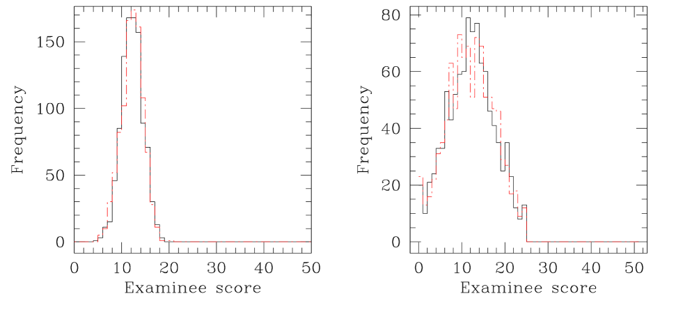
Figure 6.1: Figure showing histograms of the scores of 999 examinees in the 2 sub-tests (in solid and broken lines respectively), obtained by splitting the simulated test data set $D_{3}$ which has been generated under the choice that examinee ability is normally distributed (right panel). The left panel includes histograms of the 2 sub-tests that result from splitting the test data $D_{4}$ that was simulated using examinee ability as item-dependent, with probability for correct response to the $j$-th item given as a normal variate, unrealistically fixed for all examinees, $\forall\>j=1,\ldots,50$.

The reliabilities of tests with data $D_{1}$ and $D_{3}$ are as expected high, while the same for the infeasible tests $D_{2}$ and $D_{4}$ are low, as per prediction. We take these results as a form of validation our method of computing $r_{tt}$ based on the splitting of a test.

In Figure 6.1, we present the histograms of the 2 sub-tests that result from splitting the realistic data $D_{3}$ as well histograms of the 2 sub-tests that result from the splitting of the unrealistic test data $D_{4}$.

6.1 Results from Large Simulated Tests

We also conducted a number of experiments with finding reliabilities of larger test data sets that were simulated. The simulations were performed such that the test score variable has a Bernoulli distribution with parameter $p$. in these simulations, we chose $p_{i}$ as fixed for the $i$-th examinee, with $p_{i}$ randomly sampled from a chosen Gaussian $pdf$, i.e. $p_{i}\sim{\cal N}(0.5,0.2)$ by choice, $i=1,\ldots,N$. We simulated different test score data sets in this way, including

1. a test data set for 5$\times$10⁵ examinees taking a 50-item test.

2. a test data set for 5$\times$10⁴ examinees taking a 50-item test.

3. a test data set for 1000 examinees taking a 100-item test.

4. a test data set for 1000 examinees taking a 1000-item test.

In each case, the test data was split using our method and reliability of the test was computed as per the classical definition. The 4 simulated test data sets mentioned above, yielded reliabilities of 0.96, 0.98, 0.93, 0.85, in order of the above enumeration. Histograms of the sub-tests obtained by splitting each test data were over-plotted to confirm their concurrence.

Importantly, the run-time of reliability computation of these large cohorts of examinees ($N$=500,000 and 50,000), who take the 50-item long test, is very short–from about 0.8 seconds for the 50,000 cohort to about 6.2 seconds for the 500,000 cohort. On the other hand the order of our splitting algorithm being ${\cal O}((n/2)^{2})$, the run-times increase rapidly for the 1000-item test, from the 100-item one, with the fixed examinee number. These experiments indicate that the computation of reliabilities for very large cohorts of examinees, in a test with a realistic number of items, is rendered very fast indeed, using our method.

7 Application to real data

We apply our method of computing reliability using the classical definition, following the splitting of a real test into 2 parallel halves by the method discussed in Section 4.2. We also estimate the true scores and offer the error in this estimation, using the computed reliability and a real test score data set. The used real test data was obtained by examining 912 examinees in a multiple choice examination administered with the aim of achieving selection to a position. The test had 50 items and maximum time given was 90 minutes. To distinguish between this real test data and other real test data sets that we will employ to determine reliability of a battery, we refer to the data set used in this section as DATA-I. For the real test data DATA-I, the histograms of the item scores and that of the examinee scores are shown in Figure 7.1. The histogram of the examinee scores shows that $X_{i}\leq 26\>\forall i=1,\ldots,912$, with the biggest mode of the score distribution around 11. In other words, the test was a low-scoring one. DATA-I indicates 2 other smaller modes at about 15 and 22. Some other parameters of the test data DATA-I are as listed below.

1. number of items $n$=50,

2. number of examinees is $N$=912,

3. magnitude of the vector of maximum possible scores is $\parallel\boldsymbol{I}\parallel$ = $\sqrt{912\times 50^{2}}\approx 1509.97$,

4. magnitude of the observed score vector is $\parallel\boldsymbol{X}\parallel\approx$ 357.82,

5. $\parallel\boldsymbol{X}\parallel^{2}$ = 128032,

6. $\cos\theta_{X}\approx$0.9275

7. test mean ${\bar{X}}\approx$10.99,

8. test variance $S_{X}^{2}=\approx 19.63$.

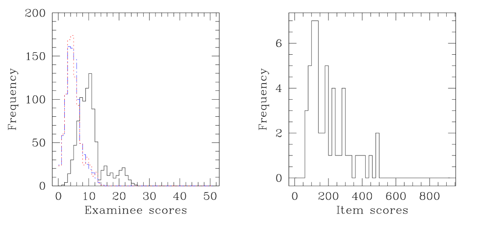
Figure 7.1: Figure showing histograms of the 912 examinee scores (left panel) and of 50 item scores (right panel) of the real test data DATA-I that we use to implement our method of splitting the test, aimed at computation of reliability as per the classical definition. The left panel also includes histograms of the $g$ and $h$ sub-tests that result from the splitting of this test; the histograms of the sub-tests are shown in dotted and dashed-dotted lines, superimposed on the histogram of examinee scores for the full test (in solid black line).

Figure 7.2: Figure showing regression of the examinee scores in the sub-test $g$ on the scores in sub-test $h$ (right panel) and vice versa (left panel), where the 2 sub-tests are obtained by splitting real data DATA-I with our method of dichotomisation (Section 4.2). The score data are shown in filled circles while the regression lines are also drawn. The regression coefficients are marked on the top left hand corner of the respective panel.

The test was dichotomised into parallel halves by the iterative process discussed in Section 4.2. Let the resulting sub-tests be referred to as the $g$ and $h$ sub-tests. Then each of these sub-tests had 25 items in it and sum of examinee scores is $\displaystyle{\sum\limits_{i=1}^{912}X_{i}^{(g)}}=\displaystyle{\sum\limits_{i=1}^{912}X_{i}^{(h)}}=5011$, so that the mean of each of the two sub-tests is equal to about 5.49. Also, variances of the 2 sub-tests are approximately equal at 6.81 and 6.49. The histograms of the examinee scores in these 2 sub-tests are drawn in blue and red in the left panel of Figure 7.1. That the histograms for the $g$ and $h$ sub-tests overlap very well, is indicative of these sub-tests being strongly parallel. We regress the score vector $(X_{1}^{(g)},\ldots,X_{912}^{(g)})^{T}$ on the score vector $(X_{1}^{(h)},\ldots,X_{912}^{(h)})^{T}$; the regression lines are shown in the right panel of Figure 7.2. Similarly, regressing $(X_{1}^{(h)},\ldots,X_{912}^{(h)})^{T}$ on the score vector $(X_{1}^{(g)},\ldots,X_{912}^{(g)})^{T}$ results in a similar linear regression line (shown in the left panel of Figure 7.2). Table 2 gives the details of splitting of the 50 items of the full test into the 2 sub-tests.

Table 2: Splitting of real data DATA-I of a selection test with 50 items, administered to 912 examinees. The dichotomisation has been carried out according to the algorithm discussed in Section 4.2.

$g$-th sub-test		$h$-th sub-test		Difference between scores of 2 tests
Score	Item No.	Score	Item no.
75	25	75	1	0
84	39	80	46	4
85	43	90	24	-5
100	20	96	9	4
102	44	103	34	-1
111	50	106	31	5
112	5	113	41	-1
124	32	115	45	9
127	36	128	8	-1
131	33	129	26	2
134	18	135	3	-1
151	29	144	4	7
172	7	178	48	-6
193	19	190	21	3
195	37	196	14	-1
205	28	199	47	6
221	30	230	6	-9
239	27	236	49	3
256	11	263	12	-7
284	2	285	17	-1
292	22	294	10	-2
337	15	309	23	28
393	13	376	42	17
405	16	453	38	-48
483	35	488	40	-5
Sum of item scores	5011		5011
Sum of squares of item scores	33453		33747

7.1 Computation of reliability

We implement the splitting of the real test score data into the scores in the $g$ and $h$ sub-tests to compute the reliability as per the theoretical definition, i.e. as given in Equation 4.6. Then using the observed sub-test score vectors $\boldsymbol{X}^{(g)}$ and $\boldsymbol{X}^{(h)}$ we get the classically defined reliability to be $r_{tt}\approx 0.66$. Then $r_{XT}:=\sqrt{r_{tt}}\approx 0.8128$. On the other hand, the Pearson product moment correlation between $\boldsymbol{X}^{(g)}$ and $\boldsymbol{X}^{(h)}$ is $r_{gh}\approx$0.9941. In other words, the split-half reliability is $r_{gh}\approx 0.9941$.

We can now proceed to estimate the true scores following the discussion presented in Section 4.4. For the observed score $X_{i}$, the estimated true score is ${\widehat{T}_{i}}=\beta_{1}X_{i}+\alpha_{1}$ (as per Equation 4.21 and discussions thereafter), where $\beta_{1}=r_{tt}$ and $\alpha_{1}={\bar{X}}(1-\beta_{1})$. The true scores can also be estimated using the split-half reliability instead of the reliability from the classical definition. Then the above regression coefficients $\beta_{q}$ and $\alpha_{q}$ are computed as above, except this time, $r_{tt}$ is replaced by $r_{gh}$, $q=1,2$. We present the true scores estimated using both the reliability from the classical definition (${\widehat{T}}_{classical}$ in black) as well as the split-half reliability (${\widehat{T}}_{split-half}$ in red) in Figure 7.3. In this figure, the errors in the estimated true scores are superimposed as error bars on this estimate, in respective colours. This error is considered to be $\pm S_{E}$, where the error variance is $S_{E}^{2}=(1-r_{tt})S_{X}^{2}$ when the classically defined reliability is implemented and $S_{E}^{2}=(1-r_{gh})S_{X}^{2}$ when the split-half reliability is used.

In fact, the method of using $r_{gh}$ in the estimation of the true scores will result in the true scores ${\widehat{T}}_{split-half}$ being over-estimated for $X>{\bar{X}}$ and under-estimated for $X<{\bar{X}}$, as shown in Theorem 4.3. This can be easily corroborated in our results in Figure 7.3; the higher value of $r_{gh}$ (than of $r_{tt}$) results in ${\widehat{T}}_{split-half}\geq{\widehat{T}}_{classical}$ for $X>{\bar{X}}$ and in ${\widehat{T}}_{split-half}\leq{\widehat{T}}_{classical}$ for $X<{\bar{X}}$.

Figure 7.3 also includes the sample probability distribution of the point estimate of the true score obtained from the linear regression model suggested in Equation 4.21, given the observed scores and using $r_{tt}$ and $r_{gh}$, i.e. $\Pr(T\leq t|r,\boldsymbol{X})$, where $r$ is the reliability. We invoke the lookup table that gives the examinee indices corresponding to a point estimate of the true score. Then the percentile rank of all those examinees whose true score is (point) estimated as $T$, is given as $100\times\Pr(T\leq t|r,\boldsymbol{X})$. (This lookup table is not included in the text for brevity’s sake). For example, the true score ${\widehat{T}}_{split-half}\in[20,21)$ is estimated using $r=r_{gh}$, for examinees with indices 893, 867, 210, 837, 834, 408, 706, 690, 655, 653, 161, 638, 312, 308, 149, 290, 539, 260. Then the percentile rank of all these examinees is about 93.

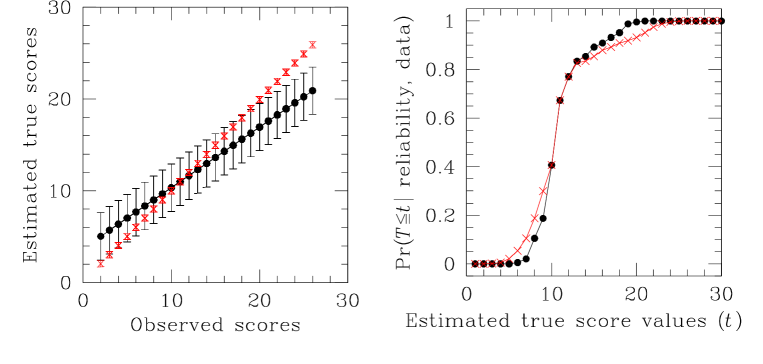
Figure 7.3: Left: figure showing the true scores estimated at observed examinee scores of the real test data DATA-I. The true scores estimated using the reliability computed from the classical definition is shown in black filled circles; the corresponding estimates of the error scores are superimposed as error bars. The true scores estimated using the split-half reliability are plotted in red crosses, as are the corresponding error scores. Right: the sample cumulative probability distributions of point estimate of true scores obtained from the linear regression model given in Equation 4.21 where implementation of the classically defined reliability results in the plot in black circles while that obtained using split-half reliability is in red crosses. This cumulative distribution can be implemented to identify the percentile rank of an examinee, in conjuction with the lookup table containing the ranking of examinee indices by the point estimate of the true score.

Thus, our method of splitting the test into 2 parallel halves helps to find a unique measure of reliability as per the classical definition, for a given real data set. Using this we can then estimate true scores for each observed score in the data.

7.2 Weighted battery score using real data

In order to illustrate our method of finding weights relevant to the computation of the classically defined weighted reliability of a test battery (Equation 5.7), we employ real life test data sets DATA-II(a) and DATA-II(b). These data sets comprise the examinee scores of 784 examinees who took 2 tests (aimed at selection for a position). The test that resulted in DATA-II(a) aimed at measuring examinee verbal ability, while the test for which DATA-II(b) was the result, measured ability to interpret data. The former test contained 18 items and the latter 22 items. Histograms of examinee scores and item scores of these 2 tests are shown in Figure 7.4. The mean and variance of the 2 tests corresponding to DATA-II(a) and DATA-II(b) are approximately 4.30, 6.25 and 4.20, 4.06 respectively. The battery comprising these two tests is considered for its reliability.

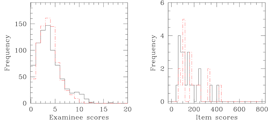
Figure 7.4: Left: figure showing histograms of the examinee scores in the tests, the scores of which constitute data sets DATA-II(a) (in black) and DATA-II(b) (in red dotted line). Right: figure showing histograms of item scores in real data DATA-II(a) (in black solid lines) and in DATA-II(b) (in red broken lines).

We split each test into 2 parallel halves using our method of dichotomisation delineated in Section 4.2. Splitting DATA-II(b) results in 2 halves, the means of the examinee scores of which are about 2.10 and the variances of the examinee scores are about 1.80 and 1.65. Reliability defined classically (Equation 4.6) computed using these split halves is about 0.35. The correlation between the split halves is about 0.90. On the other hand, splitting DATA-II(a) results in 2 halves, the means of which are equal to about 2.15 and the variances of which are about 1.87 and 2.19. Classically defined reliability of this test using these split halves, turns out be 0.66 approximately. The correlation coefficient between the two halves is about 0.95. The true scores estimated for both observed data sets are shown in Figure 7.5, with errors of estimation superimposed as $\pm S_{E}$ where $S_{E}^{2}$ is the variance of the error scores that are modelled as distributed as ${\cal N}(0,S_{E}^{2})$.

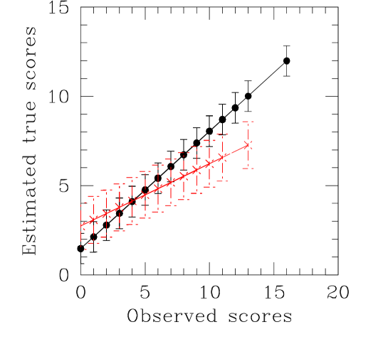
Figure 7.5: Figure showing true scores estimated using the observed scores in real data set DATA-II(a) (in black filled circles) and in DATA-II(b) (in red crosses). Errors of estimate are depicted as error bars that correspond to $\pm(1-r_{tt})^{2}S_{X}^{2}$ where the $r_{tt}$ is the classically defined reliability computed using the respective real data set.

Using the scores in the 2 tests in the considered battery, namely sets DATA-II(a) and DATA-II(b), we compute the variance-covariance matrix $\boldsymbol{D}$ of the observed scores (see Equation 5.8). Then in this example, $\boldsymbol{D}$ is a 2$\times$2 matrix, the diagonal elements of which are the variances of the 2 tests and the off-diagonal elements are the covariances of the examinee test score vectors $\boldsymbol{X}_{1}$ and $\boldsymbol{X}_{2}$ of these 2 tests. Then in this example real-life test battery, recalling that $\boldsymbol{e}=\displaystyle{\left(1,1\right)^{T}}$ we get

$$\boldsymbol{D}\approx\left(\begin{array}[]{cc}6.24&2.46\\ 2.46&4.06\end{array}\right),\quad\mbox{so that}\quad\boldsymbol{D}^{-1}\boldsymbol{e}\approx\displaystyle{\left(0.08,0.20\right)^{T}},\quad\boldsymbol{e}^{T}\boldsymbol{D}^{-1}\boldsymbol{e}\approx 0.28.$$

Then the weights are $\approx$ 0.7028 and 0.2972 (to 4 significant figures).

Then recalling that (upto 4 decimal places) the reliability and test variance of the 2 tests the score data of which are DATA-II(a) and DATA-II(b) are 0.6571, 6.2405 and 0.3488, 4.0571 respectively, the covariance between the 2 tests is 2.4571, we use Equation 5.7 to compute the reliability of this real battery to be approximately

$${\frac{0.6571\times 6.2405\times 0.7028^{2}+0.3488\times 4.0571\times 0.2972^{2}+2\times 0.7028\times 0.2972\times 2.4571}{0.7028^{2}\times 6.2405+0.2972^{2}\times 4.0571+2\times 0.7028\times 0.2972\times 2.4571}}\approx 0.7112.$$

Thus, using our method of splitting a test in two parallel halves, we have been able to compute reliability of the test as per the classical definition and extended this to compute the reliability of a real battery comprising two tests. For the used real data sets DATA-II(a) and DATA-II(b), the battery reliability turns out to be about 0.71.

8 Summary $\&$ Discussions

The paper presents a new, easily calculable split-half method of achieving reliability of tests, using the classical definition where the basic idea implemented is that the square of the magnitude of the difference between the score vectors $\boldsymbol{X}_{g}$ and $\boldsymbol{X}_{h}$ of $N$ examinees in the $g$ and $h$ sub-tests obtained by splitting the full test, is proportional to the variance $S_{E}^{2}$ of the errors in the scores obtained by the examinees who take the test, i.e. $\parallel\boldsymbol{X}_{g}-\boldsymbol{X}_{h}\parallel^{2}=NS_{E}^{2}$. Here, working within the paradigm of Classical Test Theory, the error in an examinee’s score is the difference between the observed and true scores of the examinee. Our method of splitting the test is iterative in nature and has the desirable properties that the sample distribution of the split halves are nearly coincident, indicating the approximately equal means and variances of the split halves. Importantly, the splitting method that we use, ensures maximum split-half correlation between the split halves and the splitting is performed on the basis of difficulty of the items (or questions) of the test, rather than examinee attributes. A crucial feature of this method of splitting is that the splitting being in terms of item difficulty, the method requires very low computational resources to split a very large test data set into two nearly coincident halves. In other words, our method can easily be implemented to find the classically defined reliability using test data that is obtained by collating responses from a very large sample of examinees, on whom a test of as large or as small a number of items has been administered. In our demonstration of this method, a moderately large real test on 912 examinees and 50 items, convergence to optimum splitting (splitting into halves that share equal means and nearly equal variances) was achieved in about 0.024 seconds. Implementation of sets of toy data, generated under different model choices for examinee ability was undertaken: 999 examinees responding to a 50-item test, as well as much larger cohorts of examinees–500,000 to 50,000–taking a 50-item test, and a cohort of 1000 examinees taking 100 to 1000-item tests. The order of our splitting algorithm is corroborated to be quadratic in half of the number of items in the test, while computational time for reliability computation (input+output times, in addition to splitting of the test) varies linearly with examinee sample size, so that even for the 500,000 examinees taking the 50-item test, reliability is computed to be less than 10 seconds. Once the reliability of the test is computed, it is exploited to perform interval estimation of the true score of each examinee, where the error of this estimation is modelled as the test error variance.

Subsequent to the dichotomisation of the test, we invoke a simple linear regression model for the true score of an examinee, given the observed score $X$, to achieve an interval estimate of the true score, where the interval is modelled as $\pm 1S_{E}$. We recognise this interval to be in excess of $\pm 1$ standard deviation of the error of estimation of the true score for a given $X$, as provided by the regression model; in other words, our estimation of uncertainty on the estimated true score is pessimistic.

This method of splitting a test into 2 parallel halves, forms the basis of our computation of the reliability of a battery, i.e. a set of tests, as per the classical definition. A weighted battery score is used in this computation where we implement a new way for the determination of the weights, by invoking a Lagrange multiplier based solution. We illustrate the implementation of this method of determining weights–and thereby of computing the reliability of a test battery following the computation of the reliabilities of the component test as per the classical definition–on a real test battery that comprises 2 component tests.

We have presented a new method of computing reliability as per the classical definition, and demonstrated its proficiency and simplicity. Thus, it is possible to uniquely find test characteristics like reliability or error variance from the data, and such can be adopted while reporting the results of the administered test. In this paradigm, testing of hypothesis of equality of error variance from two tests will help to compare the tests.