Parallelized Stochastic Cutoff Method for Long-Range Interacting Systems
Abstract
We present a method of parallelizing the stochastic cutoff (SCO) method, which is a Monte-Carlo method for long-range interacting systems. After interactions are eliminated by the SCO method, we subdivide a lattice into noninteracting interpenetrating sublattices. This subdivision enables us to parallelize the Monte-Carlo calculation in the SCO method. Such subdivision is found by numerically solving the vertex coloring of a graph created by the SCO method. We use an algorithm proposed by Kuhn and Wattenhofer to solve the vertex coloring by parallel computation. This method was applied to a two-dimensional magnetic dipolar system on an square lattice to examine its parallelization efficiency. The result showed that, in the case of , the speed of computation increased about times by parallel computation with processors.
1 Introduction
It is widely recognized that the recent trend in computational physics is parallel computing with a large number of computational resources. This recognition is supported by the fact that all of the top 100 supercomputers released in November 2014 consist of more than ten thousand cores. [1] Furthermore, computation with a graphics processing unit (GPU) has been a hot topic in recent years [2, 3, 4, 5, 6, 7, 8, 9, 10] because it enables us to perform massively parallel computing at a fraction of the cost. To fully utilize these parallel architectures, the development of efficient parallel algorithms is indispensable. Such parallel algorithms are required particularly in long-range interacting systems because of their high computational cost.
One example in which the parallelization of computation has been successfully achieved is the molecular dynamic (MD) method (see Refs. \citenHeffelfinger00,Larsson11, and references therein). If there are only short-range forces, parallel computations are performed by dividing the simulation box into cubic domains and assigning each domain to each processor [13]. If the system involves long-range forces such as the Coulomb ones, long-range forces for all the molecules are efficiently calculated with or computational time ( is the number of molecules) by sophisticated methods such as the Barnes-Hut tree algorithm, [14, 15, 16] first multipole method, [17, 18] and particle mesh Ewald method. [19, 20] Because these methods can be parallelized, it is possible to perform parallel computations in the MD methods even in the presence of long-range forces.
The main reason why parallel computations in the MD methods are relatively simple lies in their simultaneous feature. In the MD methods, forces acting on all the molecules are calculated at the beginning of each step, and new positions of molecules in the next time step are determined simultaneously using forces calculated in advance. In contrast, in a normal Monte-Carlo (MC) method, elements such as particles and spins are moved one at a time. This sequential feature of the MC method makes parallelization difficult. If the system involves only short-range interactions, it is still possible to perform parallel computations in the MC method. For example, MC simulations in lattice systems can be parallelized by a checkerboard decomposition. [21] Even in off-lattice systems, parallel computations are still possible by a spatial decomposition method. [22, 23, 24, 25] The spatial-decomposition technique is also used in the kinetic (event-driven) MC method in short-range interacting systems to parallelize the computation. [26, 27, 28, 29] However, such a spatial-decomposition method does not work in long-range interacting systems because all the elements interact with each other. Furthermore, the above-mentioned efficient algorithms used in the MD method to calculate long-range forces do not work in the MC method because these methods calculate long-range forces (and potentials) for all the elements at once. In the MC methods, long-range forces calculated for all the elements become invalid after a part of the elements are updated because of the sequential feature of the MC method. Therefore, it is difficult for long-range interacting systems to perform parallel computations in a normal (and most widely applicable) single-update MC method.
To overcome this difficulty, we utilize the stochastic cutoff (SCO) method. [30, 31, 32] The SCO method is a Monte-Carlo method for long-range interacting lattice systems. The basic idea of the method is to switch long-range interactions stochastically to either zero or a pseudointeraction using the Stochastic Potential Switching (SPS) algorithm [33, 34]. The SPS algorithm enables us to switch the potentials with the detailed balance condition strictly satisfied. Therefore, the SCO method does not involve any approximation. Fukui and Todo have developed an efficient MC method based on a similar strategy using different pseudointeractions and different way of switching interactions [35]. Because most of the distant and weak interactions are eliminated by being switched to zero, the SCO method markedly reduces the number of interactions and computational time in long-range interacting systems. For example, in a two-dimensional magnetic dipolar system, to which we will apply our MC method later, the number of potentials per spin and the computational time for a single-spin update are reduced from to .
This reduction of potentials also makes it possible to subdivide the lattice into noninteracting interpenetrating sublattices, i.e., so that the elements on a single sublattice do not interact with each other. This subdivision enables us to parallelize the computation. However, one problem is that there is no trivial way of finding such a subdivision. In the case of Ising models on a square lattice with nearest-neighbouring interactions, the checkerboard decomposition is responsible for it. In contrast, there is no trivial subdivision in the this case because interactions are stochastically switched. To resolve this problem, we numerically solve the vertex coloring on a graph created by the potential switching procedure. This computation is performed in a parallel fashion using an algorithm proposed by Kuhn and Wattenhofer. [36, 37]
The paper is organized as follows: In Sect. 2, we briefly explain the SCO method and describe the parallel computation of the vertex coloring, which is a key feature of the present method. In Sect. 3, we show the results obtained by applying the present method to a two-dimensional magnetic dipolar system. In Sect. 4, we give our conclusions.
2 Methods
2.1 Stochastic Cutoff (SCO) Method
In this subsection, we briefly explain the SCO method. We consider a system with pairwise long-range interactions described by a Hamiltonian , where is a variable associated with the -th element of the system. In the SCO method, is stochastically switched to either or a pseudointeraction as
| (1) |
The probability and the pseudointeraction are given by
| (2) |
| (3) |
where is the inverse temperature and is a constant equal to (or greater than) the maximum value of over all and . With this potential switching, the algorithm proceeds as follows:
-
(A)
Switch the potentials to either or with the probability of or , respectively.
-
(B)
Perform a standard MC simulation with the switched Hamiltonian
(4) for MC steps, where runs over all the potentials switched to and one MC step is defined by one trial for each to be updated.
-
(C)
Return to (A).
In the SCO method, an efficient method is employed to reduce the computational time of the potential switching in step (A) (see Ref. \citenSCO for details). As a result, the computational time in step (A) becomes comparable to that in step (B) per MC step. For example, in the case of a two-dimensional magnetic dipolar system, both computational times are reduced to .
2.2 Outline of parallel computations of the SCO method
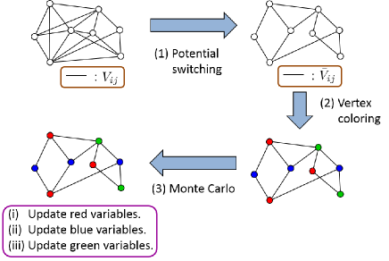
Figure 1 shows a schematic illustration of parallel computations of the SCO method. A vertex denotes a variable and an edge denotes a potential or . In step (1), each potential is switched to either or . The edges whose potentials are switched to are eliminated in the subsequent steps. Because each potential is switched independently with the probability , we can easily parallelize the computation in this step. In step (2), the vertex coloring of the graph created in step (1) is solved numerically in a parallel fashion. The parallel computation of the vertex coloring will be explained in detail in the next subsection. Lastly, we perform a standard MC simulation with the switched Hamiltonian in step (3). It is apparent from the definition of the vertex coloring that variables with the same color do not interact with each other. Therefore, we can update variables with a specific color by parallel computation, as we do in MC simulations of Ising models by a checkerboard decomposition. By doing this simultaneous update for all the colors, we can parallelize the MC calculation in step (3).
2.3 Parallel computation of the vertex coloring
In this subsection, we briefly explain parallel computation of the vertex coloring. We refer the reader to the book in Ref. \citenbook_KW for more details. By solving the vertex coloring in a parallel fashion, we can perform all the three steps mentioned in the previous subsection by parallel computation. We hereafter call the vertex coloring by parallel computation distributed graph coloring.
The organization of this subsection is as follows: In Sect. 2.3.1, we explain the basis of the distributed graph coloring. In Sect. 2.3.2, we explain a basic color reduction algorithm for the distributed graph coloring. This algorithm is used in an algorithm proposed by Kuhn and Wattenhofer, [36, 37] which is used in this study. This algorithm is explained in Sect. 2.3.3.
2.3.1 Basis of the distributed graph coloring
We start with the introduction of several technical terms in the graph theory. The degree of a vertex is the number of edges that connect the vertex with others, and the maximum degree is the largest value of the degrees of a graph. In general, it is known that a graph with a maximum degree can be colored with colors, while, in most cases, it is not the smallest number of colors needed to color the graph. The aim of the distributed graph coloring is to color a graph with colors by parallel computation.
In the distributed graph coloring, each vertex is initially colored by different colors, i.e., a graph is colored with colors, where is the number of vertices. The number of colors is gradually reduced from to by repeating synchronous communication and parallel computation. In synchronous communication, vertices communicate with each other to know the colors of their neighbouring vertices. In parallel computation, all vertices simultaneously recolor themselves. The new color is locally calculated by using the information of the neighbouring colors obtained in the preceding communication. Vertices do not communicate with each other in parallel computation. The number of times of synchronous communications required to accomplish a -coloring is called running time, hereafter denoted as . The main aim of the distributed graph coloring is to reduce as much as possible.
2.3.2 Basic color reduction algorithm
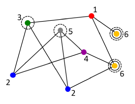
The basic color reduction (BCR) algorithm is one of the most fundamental algorithms for the distributed graph coloring. Figure 2 shows a graph and its coloring to which we apply the BCR algorithm. We assume that the number of vertices and the maximum degree of the graph are and , respectively. The graph is initially colored with colors and the coloring is valid, i.e., no adjacent vertices share the same color. The color of a vertex is specified by an integer between 1 and . In the BCR algorithm, the number of colors is reduced from to by the following steps: [38]
-
(1)
Each vertex communicates with each other to obtain the colors of the neighbouring vertices.
-
(2)
Each vertex recolors itself if its color is . The new color is chosen from a palette between and by using the information obtained in step (1).
Steps (1) and (2) correspond to synchronous communication and parallel computation in the previous subsection, respectively. We can always choose a new color among colors because the maximum degree of the graph is . It is also important to notice that the vertices with the color cannot be adjacent to each other because the initial coloring is valid (see the vertices enclosed by a solid circle in Fig. 2). This means that the new coloring is also valid even if each vertex with the color simultaneously changes its color according to the information of the neighbouring colors. The BCR algorithm reduces the number of colors one at a time by repeating these two steps. Therefore, the running time to accomplish a -coloring from an initial -coloring is .
When we implemented the BCR algorithm in our simulation, we slightly modified the algorithm to improve its efficiency. To be specific, we modified step (2) in the following manner:
-
(2)’
Each vertex recolors itself if its color is locally maximum. The new color is chosen from a palette between and using the information obtained in step (1).
In Fig. 2, the vertices recolored in steps (2)’ and (2) are enclosed by dashed circles and solid ones, respectively. We see that the former involves the latter. This means that the running time is reduced by this modification. We also find in Fig. 2 that the vertices recolored in step (2)’ are not adjacent to each other because they are locally maximum. Therefore, the new coloring is also valid by the same reason as before. A demerit of this modification lies in the computational cost to check whether the color of a vertex is locally maximum. However, this demerit was not significant in our simulations because the degrees of graphs were not so large.
2.3.3 KW algorithm
In this subsection, we explain an algorithm proposed by Kuhn and Wattenhofer. [36] We hereafter call it the KW algorithm. The KW algorithm markedly reduces the running time by applying the BCR algorithm recursively. As mentioned above, we used this algorithm to numerically solve the vertex coloring.
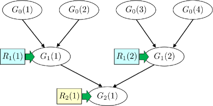
Figure 3 shows a schematic illustration of the KW algorithm. For simplicity, we assume that the number of vertices and the maximum degree are related by , where is an integer. Generalization to other cases is straightforward. We suppose that all the vertices are initially colored by different colors. The color is specified by an integer between and . The KW algorithm starts by partitioning all vertices into groups according to their colors. We hereafter denote them by , where the subscript “0” represents the level of the grouping. In this partitioning, vertices whose color is between and are assigned to the -th group . We next make groups at level by integrating two adjacent groups at level (see Fig. 3). We denote them by . Just after the integration, vertices in the group are colored by colors. We then apply the BCR algorithm to reduce the number of colors from to . We denote this color reduction applied to vertices in the group by . We can simultaneously perform all the color reductions at level because there is no overlap of colors among the groups. In the color reduction , the color of vertices is changed so that the new color is between and . This guarantees that there is no overlap of colors among groups at level even after the color reductions. As a result of all the color reductions at level , the number of colors used for coloring the whole graph is reduced from to . By repeating the integration of two adjacent groups and the subsequent parallel color reduction times, the number of colors is reduced to .
We next consider the running time of the KW algorithm. At a level , there are groups. In each group, the number of colors is reduced from to by the BCR algorithm. Now, the point is that we can simultaneously perform BCRs in all the groups. To be specific, we simultaneously perform BCRs in all the groups to reduce the number of colors by one, and perform synchronous communication just once for the next color reductions. By repeating this procedure times, we can reduce the numbers of colors of all the groups from to . The running time to achieve this color reduction at the level is . Because the number of levels is , the total running time to reduce the number of colors from to is estimated to be
| (5) |
where we have used the relation . If , this running time is much shorter than that of the BCR algorithm, which is, as mentioned above, on the order of .
3 Results
3.1 Model
To investigate the efficiency of parallel computation of the method developed in this study, we apply the method to a two-dimensional magnetic dipolar system on an square lattice with open boundaries. The Hamiltonian of the system is described as
| (6) |
where is a classical Heisenberg spin of , runs over all the nearest-neighbouring pairs, is the vector spanned from a site to in the unit of the lattice constant , and . The first term describes short-range ferromagnetic exchange interactions and the second term describes long-range dipolar interactions, where is an exchange constant and is a constant that represents the strength of magnetic dipolar interactions. We hereafter consider the case that . We choose this model because it was used as a benchmark of the SCO method. [30] It is established that the model undergoes a phase transition from a paramagnetic state to a circularly ordered state at as a consequence of the cooperation of exchange and dipolar interactions. [39] We applied the SCO method only for magnetic dipolar interactions. The system was gradually cooled from an initial temperature to in steps of . The initial temperature was set to be well above the critical temperature. We set defined in Sect. 2.1 to be , i.e., potential switching and subsequent vertex coloring are performed every MC steps. It was determined in Ref. \citenSCO that this frequency of potential switching is sufficient for this model to obtain reliable results.
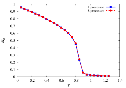
To check the correctness of our parallel computation, we performed MC simulation and measured the absolute value of the circular component of magnetization defined by
| (7) |
where denotes the -component of a vector, denotes thermal average, and is a vector describing the center of the lattice. In this measurement, the system was kept at each temperature for MC steps. The first MC steps are for equilibration and the following MC steps are for measurement. We performed simulations for different runs with different initial conditions and random sequences. The result is shown in Fig. 4. The squares and circles denote the result of single-thread computation with processor and that of multiple-thread computation with processors, respectively. Both data coincide with each other within statistical error. We also see that rapidly increases around the critical temperature . From these results, we conclude that our parallel computation is performed correctly.
| temperature | ||
|---|---|---|
| 1.40 | 8.54 | |
| 3.36 | 12.9 | |
| 22.7 | 41.6 |
3.2 Properties of graphs and improvements to reduce communication traffic
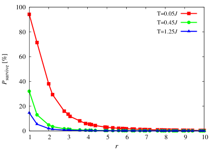
In Table 1, we show the mean degree and the maximum degree of graphs at three temperatures. These are important quantities because the maximum degree determines the number of colors and the mean degree is proportional to the computational time per MC step. The size is . As found in Ref. \citenSCO, these quantities hardly depend on the size in two-dimensional magnetic dipolar systems if the size is sufficiently large. As expected from Eq. (2), both and increase with decreasing temperature. However, they are several tens at most. This means that most of the interactions are cut off by the potential switching. It should be noted that both and are before potentials are switched. Figure 5 shows the distance dependence of the probability that a potential survives by being switched to . The temperatures are the same as those in Table 1. We see that the probability increases with decreasing temperature. The probability is close to one when and . However, rapidly decreases with increasing at any temperature.
Taking these properties of the SCO method into consideration, we implemented our simulation in the following way: We first divide a lattice into square cells ( is the number of processors) and assign each cell to each processor. We then list the vertices whose information should be sent by interprocessor communication when we update spins with a certain color. For example, a vertex is added to a list for red-spin update if it satisfies the following two conditions:
-
The vertex is connected with a red vertex .
-
The two vertices and belong to different cells.
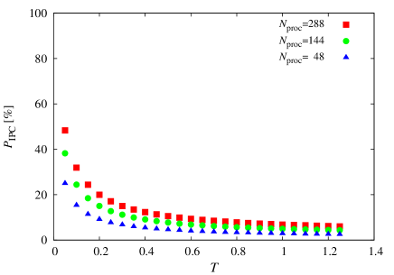
This list is made for each color just once when a new graph is created by the potential switching. When we update spins of a certain color, we perform interprocessor communication in advance according to the list. Although it requires some computational cost to make the lists, they enable us to reduce the communication traffic before parallel MC calculation as much as possible. Figure 6 shows the temperature dependence of the proportion of surviving potentials that require interprocessor communication. The proportion increases with increasing number of processors. Note that the mesh size decreases as the number of processors increases. The proportion also increases with decreasing temperature. However, it is less than in most cases, meaning that communication traffic is considerably reduced by this improvement.
3.3 Efficiency of parallel computation
In Fig. 7, we plot the average computational time per MC step as a function of the number of processors. The average time is defined by
| (8) |
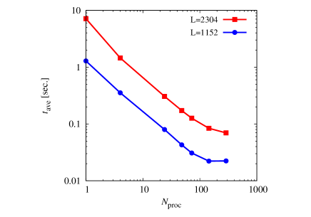
where , , and are the computational times to switch potentials, to solve vertex coloring, and to perform MC simulation for one MC step, respectively. Recall that potential switching and the subsequent vertex coloring are performed every MC steps. The average is taken over the temperatures between and . The data for and those for are denoted by squares and circles, respectively. The data correspond to the strong scaling because is increased with the system size fixed. When is , the computations with and processors are about and times faster than that with one processor, respectively. In the case of , the speedups by and processors are about and , respectively.
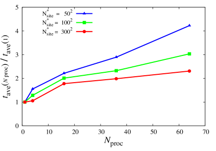
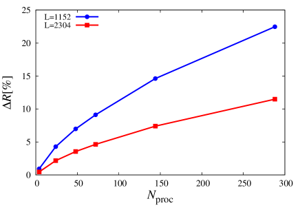
Figure 8 shows the data of the weak scaling. In the weak scaling, we increase both the system size and with the number of sites per processor fixed. In the figure, the ratio is plotted as a function of , where is the average computational time when the number of processors is . We see that the ratio decreases with increasing . This means that the parallelization efficiency is improved as the system size increases.
We next consider fluctuations in the number of sites assigned to each processor in the MC calculation. As mentioned in Sect. 3.2, when we update spins with some color in the MC calculation, each processor updates spins in the assigned cell. The number of sites with the color is different from cell to cell. Because these fluctuations cause the difference in the computational time among processors, it may significantly decrease the parallelization efficiency. To evaluate the effect of fluctuations, we measured the following quantity:
| (9) |
where and are the maximum and average values of the number of sites with a certain color, respectively. We measured this quantity because the computational time is determined by the maximum number of sites among processors. Figure 9 shows the dependence of . The average is taken over the colorings and the colors of each coloring. The temperature is . Because the number of colors increases with decreasing temperature, this temperature corresponds to the worst case. The data for and those for are denoted by circles and squares, respectively. When and , is about . This means that the fluctuations decrease the parallelization efficiency to some extent. However, we also see that the fluctuations decrease with increasing system size.
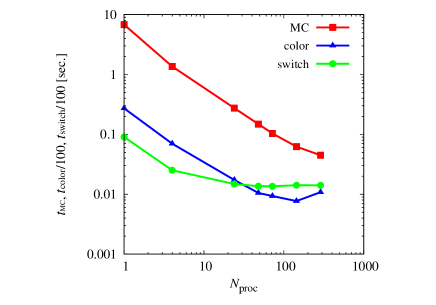
In Fig. 10, , , and are plotted as functions of the number of processors. The size is . The sum of the three computational times is equal to for shown in Fig. 7 (see Eq. (8)). The computation time of MC simulation is dominant owing to the factor in and . We see that each computational time saturates as increases. Although there are several causes of the saturation, such as the fluctuations in the number of sites discussed in the previous paragraph, the main reason for the saturation is an increase in communication traffic. In the MC calculation, we reduced communication traffic by the method described in Sect. 3.2. Therefore, the saturation of is gradual. In contrast, the proportion of communication traffic is large in the potential switching and coloring because the improvement mentioned in Sect. 3.2 is not applicable to them. To make the present method effective even for larger parallel computations, we need to improve the parallelization efficiencies of the two processes.
4 Conclusions
In this study, we have developed a method of parallelizing the SCO method, which is a MC method for long-range interacting systems. To parallelize the MC calculation in the SCO method, we numerically solve the vertex coloring of a graph created by the SCO method. This computation is performed in parallel using the KW algorithm. [36, 37] We applied this method to a two-dimensional magnetic dipolar system on an square lattice to examine its parallelization efficiency. The result showed that, in the case of , the speed of computation increased about times by parallel computation with processors.
Acknowledgments
This work was supported by JSPS KAKENHI Grant Number 25400387. Some of the experimental results in this research were obtained using supercomputing resources at Cyberscience Center, Tohoku University.
References
- [1] http://www.top500.org/
- [2] J. D. Owens, D. Luebke, N. Govindaraju, M. Harris, J. Krüger, A. E. Lefohn, and T. J. Purcell, Comput. Graph. Forum 26, 80 (2007).
- [3] J. A. Anderson, C. D. Lorenz, and A. Travesset, J. Comput. Phys. 227, 5342 (2008).
- [4] T. Preis, P. Virnau, W. Paul, and J. J. Schneider, J. Comput. Phys. 228, 4468 (2009).
- [5] M. Bernaschi, G. Parisi, and L. Parisi, Comput. Phys. Commun. 182, 1265 (2011).
- [6] Y. Komura and Y. Okabe, Comput. Phys. Commun. 183, 1155 (2012).
- [7] J. Mick, E. Hailat, V. Russo, K. Rushaidat, L. Schwiebert, and J. Potoff, Comput. Phys. Commun. 184, 2662 (2013).
- [8] J. A. Anderson, E. Jankowski, T. L. Grubb, M. Engel, and S. C. Glotzer, J. Comput. Phys. 254, 27 (2013).
- [9] M. Bernaschi, M. Bisson, and F. Salvadore, Comput. Phys. Commun. 185, 2495 (2014).
- [10] M. Baity-Jesi, L. A. Fernández, V. Martín-Mayor, and J. M. Sanz, Phys. Rev. B 89, 014202 (2014).
- [11] G. S. Heffelfinger, Comput. Phys. Commun. 128, 219 (2000).
- [12] P. Larsson, B. Hess, and E. Lindahl, WIREs Comput. Mol. Sci. 1, 93 (2011).
- [13] D. Fincham, Mol. Sim. 1, 1 (1987).
- [14] A. W. Appel, SIAM J. Sci. Stat. Comput. 6, 85 (1985).
- [15] J. Barnes and P. Hut, Nature 324, 446 (1986).
- [16] J. Makino, J. Comput. Phys. 87, 148 (1990).
- [17] L. Greengard, The Rapid Evolution of Potential Fields in Particle Systems (MIT Press, Cambridge, MA, 1988).
- [18] J. Carrier, L. Greengard, and V. Rokhlin, SIAM J. Sci. Stat. Comput. 9, 669 (1988).
- [19] T. Darden, D. York, and L. Pedersen, J. Chem. Phys. 98, 10089 (1993).
- [20] U. Essmann, L. Perera, M. L. Berkowitz, T. Darden, H. Lee, and L. G. Pedersen, J. Chem. Phys. 103, 8577 (1995).
- [21] D. P. Landau and K. Binder, A Guide to Monte Carlo Simulations in Statistical Physics (Cambridge University Press, Cambridge, 2015) 4th ed., p. 76.
- [22] G. S. Heffelfinger, M. E. Lewitt, J. Comput. Chem. 17, 250 (1996).
- [23] A. Uhlherr, S. J. Leak, N. E. Adam, P. E. Nyberg, M. Doxastakis, V. G. Mavrantzas, and D. N. Theodorou, Comput. Phys. Commun. 144, 1 (2002).
- [24] R. Ren and G. Orkoulas, J. Chem. Phys. 126, 211102 (2007).
- [25] B. Sadigh, P. Erhart, A. Stukowski, A. Caro, E. Martinez, L. Zepeda-Ruiz, Phys. Rev. B 85, 184203 (2012).
- [26] B. D. Lubachevsky, Complex Syst. 1, 1099 (1987).
- [27] G. Korniss, M. Novotny, and P. Rikvold, J. Comput. Phys. 153, 488 (1999).
- [28] E. Martínez, J. Marian, M. Kalos, and J. Perlado, J. Comput. Phys. 227, 3804 (2008).
- [29] G. Arampatzis, M. A. Katsoulakis, P. Plechác̆, M. Taufer, and L. Xu, J. Comput. Phys. 231, 7795 (2012).
- [30] M. Sasaki and F. Matsubara, J. Phys. Soc. Jpn. 77, 024004 (2008).
- [31] M. Sasaki, Phys. Rev. E 82, 031118 (2010).
- [32] p. 181 of Ref. \citenLandauBinder_checkerboard.
- [33] C. H. Mak, J. Chem. Phys. 122, 214110 (2005).
- [34] C. H. Mak and A. K. Sharma, Phys. Rev. Lett. 98, 180602 (2007).
- [35] K. Fukui and S. Todo, J. Comp. Phys. 228, 2629 (2009).
- [36] F. Kuhn and R. Wattenhofer, Proc. of the 25th ACM Symp. on Principles of Distributed Computing, 2006, p. 7.
- [37] L. Barenboim and M. Elkin, Distributed Graph Coloring: Fundamentals and Recent Developments (Morgan & Claypool Publishers, San Rafael, 2013) p. 38.
- [38] p. 29 of Ref. \citenbook_KW.
- [39] J. Sasaki and F. Matsubara, J. Phys. Soc. Jpn. 66, 2138 (1997).