Magnetic wormholes and black universes with invisible ghosts

K. A. Bronnikov^a,b,c,1 and P. A. Korolyov^b,2

^a

Center of Gravitation and Fundamental Metrology, VNIIMS, Ozyornaya St. 46, Moscow 119361, Russia

^b

Institute of Gravitation and Cosmology, PFUR, Miklukho-Maklaya St. 6, Moscow 117198, Russia

^c

I. Kant Baltic Federal University, Al. Nevsky St. 14, Kaliningrad 236041, Russia

We construct explicit examples of globally regular static, spherically symmetric solutions in general relativity with scalar and electromagnetic fields describing traversable wormholes with flat and AdS asymptotics and regular black holes, in particular, black universes. (A black universe is a regular black hole with an expanding, asymptotically isotropic space-time beyond the horizon.) The existence of such objects requires invoking scalars with negative kinetic energy (“phantoms”, or “ghosts”), which are not observed under usual physical conditions. To account for that, the se-called “trapped ghosts” were previously introduced, i.e., scalars whose kinetic energy is only negative in a restricted strong-field region of space-time and positive outside it. This approach leads to certain problems, including instability (as is illustrated here by derivation of an effective potential for spherical pertubations of such systems). In this paper, we use for model construction what we call “invisible ghosts”, i.e., phantom scalar fields sufficiently rapidly decaying in the weak-field region. The resulting configurations contain different numbers of Killing horizons, from zero to four.

1 Introduction

The existence of the so-called exotic matter, violating the weak and null energy conditions, is favored by modern cosmological observations allowing for the ratio of pressure to energy density, $w=p/\rho<-1$ (see, e.g., [1] and references therein). This is one of the reasons for the recent interest in the construction and properties of wormhole configurations in general relativity and its extensions (see, e.g., [2, 4, 3, 5] for reviews), since, as is well known, it is the necessity of exotic matter that makes a fundamental problem in wormhole construction [6].

It has also been discovered that if one admits the existence of exotic matter, for example, in the form of phantom scalar fields, then, in addition to wormholes, there can appear quite a number of other interesting and unusual configurations, such as different types of regular black holes and, among them, the so-called black universes. The latter look in the static region basically the same as “ordinary” black holes in general relativity, but beyond the horizon, instead of a singularity, they contain an expanding universe which ultimately becomes isotropic and can be asymptotically de Sitter at large times [7, 8].

Since no exotic matter or phantom fields have been detected under usual physical conditions, it is desirable to avoid the emergence of such fields in an asymptotic weak-field region. To that end, it has been suggested [9, 10, 11] to use a special kind of fields, named “trapped ghosts”, which have phantom properties only in some restricted strong-field region and satisfy the standard energy conditions in the remaining part of space. With such a field, a variety of solutions have been obtained, including regular black holes, black universes and traversable wormholes.

In all these models, the kinetic energy density smoothly passes zero at some scalar field value $\phi=\phi_{0}$, being negative at $\phi>\phi_{0}$. This transition point has certain undesirable properties, in particular, if we consider perturbations of a static, spherically symmetric configuration with such a field, the corresponding effective potential has a singularity which should in general lead to a violent instability.

Trying to avoid these problems, in this paper we consider wormhole and black universe models without a trapped ghost but use, instead, a superposition of two scalar fields, a phantom one and a canonical one, requiring a sufficiently rapid decay of the phantom field in the weak-field region. We call this design an “invisible ghost”.

We use the electromagnetic field as one more source of gravity. As in [11], we deal with static, spherically symmetric space-times, therefore the only kinds of electromagnetic fields are a radial electric (Coulomb) field and a radial magnetic (monopole) field. For the latter, it is unnecessary to assume the existence of magnetic charges (monopoles): in both wormholes and black universes a monopole magnetic field can exist without sources due the space-time geometry. In the wormhole case it perfectly conforms to Wheeler’s idea of a “charge without charge” [13], and this charge can be both electric and magnetic.

One of the motivations for including the electromagnetic field into consideration is that by modern observations there can exist a global magnetic field up to $10^{-15}$ Gauss, causing correlated orientations of sources remote from each other [14], and some authors admit a possible primordial nature of such a magnetic field.

The results obtained here show that a superposition of phantom and canonical scalar fields combined with an electromagnetic field can support wormholes, black universes and other kinds of regular black holes without a center. Actually, the set of possible types of geometry coincides with that obtained previously with the aid of a pure phantom scalar [12] or a trapped ghost [11].

The paper is organized as follows. In Section 2 we present the basic equations and make some general observations. In Section 3 we obtain examples of wormhole and regular black hole configurations supported by a superposition of two scalar fields, a phantom one and a canonical one. The Appendix presents the form of the effective potential for radial perturbations of static, spherically symmetric field systems, more general than considered here, including those with a trapped ghost.

2 Basic equations

Consider a field system with the action

$${}{\cal S}=\frac{1}{16\pi}\int\sqrt{-g}d^{4}x\Big{[}R+2h_{ab}(\partial\phi^{a},\partial\phi^{b})$$

$${}\hskip 72.26999pt-2V(\phi^{a})-F_{\mu\nu}F^{\mu\nu}\Big{]},$$ (1)

in a static, spherically symmetric space-time, where $R$ is the scalar curvature, $g=\det(g_{\mu\nu})$, $F_{\mu\nu}$ is the electromagnetic field tensor, $\{\phi^{a}\}$ is a sigma-model type set of scalar fields, $h_{ab}=h_{ab}(\phi^{a})$ is a nondegenerate target space metric, $(\partial\phi^{a},\partial\phi^{b})\equiv g^{\mu\nu}\partial_{\mu}\phi^{a}\partial_{\nu}\phi^{b}$, and $V(\phi^{a})$ is an interaction potential.

The metric can be written as

$$ds^{2}=A(u)dt^{2}-\frac{du^{2}}{A(u)}-r^{2}(u)d\Omega^{2},$$ (2)

where we use the so-called quasiglobal gauge $g_{00}g_{11}=-1$, and $d\Omega^{2}=(d\theta^{2}+\sin^{2}\theta d\varphi^{2})$ is the linear element on a unit sphere.

Our interest is in wormhole and black universe solutions, describing nonsingular configurations without a center. Hence we assume that the range of $u$ is $u\in\mathbb{R}$, where both $A(u)$ and $r(u)$ are regular, $r>0$ everywhere, and $r\to\infty$ at both ends. We also require $r(u)\approx|u|$ as $u\to\pm\infty$, which is in agreement with possible flat, de Sitter or AdS symptotic behaviors at large $r$.

The existence of two asymptotic regions with $r\sim|u|$ implies that there is at least one regular minimum of $r(u)$ at some $u=u_{0}$, at which (the prime stands for $d/du$)

$$r=r_{0}>0,\quad\ r^{\prime}=0,\quad\ r^{\prime\prime}>0.$$ (3)

The necessity of violating the weak and null energy conditions (WEC and NEC) at such minima follows from the Einstein equations. Indeed, one of them reads (see Eq. (10) below)

$$2Ar^{\prime\prime}/r=-(T^{t}_{t}-T^{u}_{u}),$$ (4)

where $T_{\mu}^{\nu}$ are components of the stress-energy tensor (SET). If a minimum of $r$ occurs in an R-region (i.e., $A>0$), it is a throat. The condition $r^{\prime\prime}>0$ implies, according to (4), $T^{t}_{t}-T^{u}_{u}<0$, or, in conventional terms, ($T^{t}_{t}=\rho$ and $-T^{u}_{u}=p_{r}$, the energy density and radial pressure, respectively) $\rho+p_{r}<0$, which manifests NEC violation. It is a simple proof for static, spherically symmetric wormhole throats ([15]; see also [3]).

If a minimum of $r$ occurs in a T-region ($A<0$), it is not a throat but a bounce in the time evolution of one of the scale factors in a Kantowski-Sachs cosmology (the other scale factor is $[-A(u)]^{1/2}$). In a T-region $t$ is a spatial coordinate, so $-T^{t}_{t}=p_{t}$ is the corresponding pressure, while $T^{u}_{u}=\rho$; however, the condition $r^{\prime\prime}>0$ in (4) leads to $\rho+p_{t}<0$, again violating the NEC. In the intermediate case of $A=0$ (a horizon) at a minimum of $r$, the condition $r^{\prime\prime}>0$ should also hold in its vicinity, with all its consequences. Thus a minimum of $r$ always implies a NEC (and hence WEC) violation.

The Einstein field equations can be written as

$$R_{\mu\nu}=2h_{ab}\partial\mu\phi^{a}\partial_{\nu}\phi^{b}-g_{\mu\nu}V+T_{\mu\nu}[F];$$ (5)

where $T_{\mu\nu}[F]$ is the SET of the electromagnetic field. Nonzero components of $F_{\mu\nu}$ compatible with the metric (2) are $F_{01}=-F_{10}$ (a radial electric field) and $F_{23}=-F_{32}$ (a radial magnetic field), and the Maxwell equations lead to

$$F_{01}F^{01}=-q_{e}^{2}/r^{4}(u),\quad\ F_{23}F^{23}=q_{m}^{2}/r^{4}(u),$$ (6)

where the constants $q_{e}$ and $q_{m}$ are the electric and magnetic charges, respectively. The corresponding SET is ($q:=\sqrt{q^{2}_{e}+q^{2}_{m}}$)

$$T_{\mu}^{\nu}[F]=\frac{q^{2}}{r^{4}(u)}\mathop{\rm diag}\nolimits(1,1,-1,1).$$ (7)

As to the scalar fields, let us assume that there are two of them, a usual, canonical field $\phi(u)$, and a phantom one, $\psi(u)$, able to provide NEC and WEC violation, so that $h_{ab}=\mathop{\rm diag}\nolimits(1,-1)$. For the potential we make the simplest assumption

$$V=V_{\phi}(\phi)+V_{\psi}(\psi),$$ (8)

thus both fields are self-interacting but do not directly interact with each other. Then the set of equations to be solved can be written as

$${}(A^{\prime}r^{2})^{\prime}=-2r^{2}V+2q^{2}/r^{2},$$ (9)

$${}r^{\prime\prime}/r=-\phi^{\prime 2}+\psi^{\prime 2},$$ (10)

$${}A(r^{2})^{\prime\prime}-r^{2}A^{\prime\prime}=2-4q^{2}/r^{2},$$ (11)

$${}2\square\phi=dV_{\phi}/d\phi,$$ (12)

$${}2\square\psi=-dV_{\psi}/d\psi,$$ (13)

where $\square$ is the d’Alembert operator: for any $f(u)$, $\square f=-r^{-2}[Ar^{2}f^{\prime}]^{\prime}$. The unknowns are $\phi(u)$, $\psi(u)$, $A(u)$, $r(u)$, as well as the potentials $V_{\phi}(\phi)$ and $V_{\psi}(\psi)$. Eq. (11) can be integrated giving

$$r^{4}B^{\prime}(u)=-2u+4q^{2}\int\frac{du}{r^{2}(u)},\quad B(u)\equiv\frac{A}{r^{2}}.$$ (14)

3 Examples of models with an invisible ghost

It is hard to solve Eqs. (9)–(13) with given potentials $V_{\phi}$ and $V_{\psi}$. Instead, following the lines of [7, 9, 10, 11, 12], we try to find examples of interest using the inverse problem method: specifying the functions $r(u)$ and $\phi(u)$, we find all other unknowns from the field equations. Given the function $r(u)$ and the charge $q$, the redshift function $A(u)$ is found from (11), and the summed potential $V(u)$ from (9). The phantom field $\psi(u)$ can be found from (10) provided $\phi(u)$ is known. Lastly, the separate potentials $V_{\phi}$ and $V_{\psi}$ are found using (12) and (13).

We can choose the function $r(u)$, providing the opportunity of wormhole and black universe configurations, in the same form as in [11]:

$$r(u)=a\frac{x^{2}+1}{\sqrt{x^{2}+n}},\qquad n={\rm const}>2,$$ (15)

where $x=u/a$, and $a>0$ is an arbitrary constant with the dimension of length. Hence,

$$r^{\prime\prime}(u)=\frac{1}{a}\frac{x^{2}(2-n)+n(2n-1)}{(x^{2}+n)^{5/2}},$$ (16)

so that $r^{\prime\prime}>0$ at $x^{2}<n(2n-1)/(n-2)$ (a behavior compatible with a phantom scalar) and $r^{\prime\prime}<0$ at larger $|x|$. It is also clear that $r\approx a|x|$ at large $|x|$. This ensures a negative kinetic energy density (see the r.h.s. of (10)) at low values of $x$ and a positive one in the rest of space. We will take $a=1$, which is in essence a choice of a length unit. The values of $r$, $q$, $m$ ($m$ is the Schwarzschild mass in our geometrized units), having the dimension of length, thus become dimensionless but are actually expressed in terms of $a$. The quantities $B(u)$ and $V(u)$ and others having the dimension (length)^-2, are expressed in units of $a^{-2}$. The quantities $A(u)$, $\phi(u)$, $\psi(u)$ are dimensionless.

From Eq. (14) it follows

$${}B^{\prime}(x)=\frac{(x^{2}+n)^{2}}{(x^{2}+1)^{4}}\biggl{[}6p-2x$$

$${}\ \ \ +2q^{2}\biggl{(}\frac{(n-1)x}{1+x^{2}}+(n+1)\arctan x\biggr{)}\biggr{]},$$ (17)

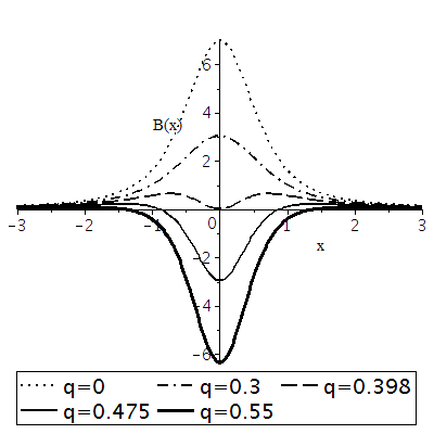
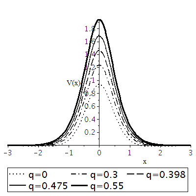
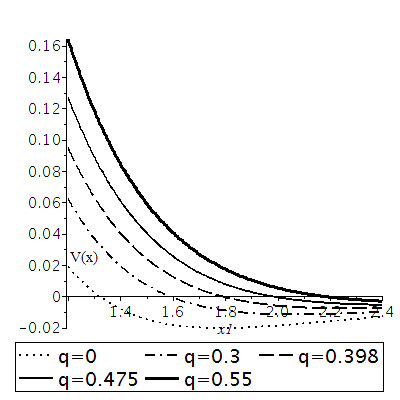
a                                                 b                                                 c

Figure 1: The function $B(x)$ (a) and the potential $V(x)$ (b, c) for symmetric configurations with $0\leq q<1$. Panel c shows that there is necessarily a region with negative values of $V$.

where $p$ is an integration constant. Further integration can be performed analytically but the resulting expressions for $B(x)$ and other quantities are too cumbersome. For definiteness, we further choose $n=4$ (one can check that other values $n>3$ do not qualitatively change the solution), then

$${}B(u)=-\frac{27}{4}\frac{q^{2}}{(x^{2}+1)^{4}}$$

$${}+\frac{1}{2}\frac{30q^{2}x\arctan(x)-7q^{2}9mx-6\pi qx+6}{(x^{2}+1)^{3}}$$

$${}+\frac{3}{16}\frac{180q^{2}x\arctan x+37q^{2}+54mx-36\pi qx+16}{(x^{2}+1)^{2}}$$

$${}+\frac{1}{16}\frac{890q^{2}x\arctan x+445q^{2}+267mx}{x^{2}+1}$$

$${}+\frac{1}{16}\frac{-178\pi qx+16}{x^{2}+1}+\frac{445}{16}q^{2}\arctan^{2}x$$

$${}+\frac{89}{16}\arctan x(-3m+2\pi q)-B_{0},$$ (18)

with an integration constant $B_{0}$. Assuming asymptotic flatness as $x\to+\infty$, that is, $A\to 1$, we should require $B=A/r^{2}\to 0$, which leads to

$$B_{0}=\frac{445}{64}\pi^{2}q^{2}-\frac{89}{16}\pi^{2}q+\frac{267}{32}\pi m$$ (19)

Comparing the asymptotic expression $A(x)=1-2m/x+o(1/x)$ with $A(x)=Br^{2}$ following from (3), the parameter $p$ is related to the Schwarzschild mass $m$ and the charge $q$:

$$p=m-\frac{2}{3}\pi q^{2}$$ (20)

Thus $B$ is a function of $x$ and two parameters, the mass $m$ and the charge $q$. Furthermore, using (9), we find the potential $V(x)$ depending on the parameters $m$ and $q$.

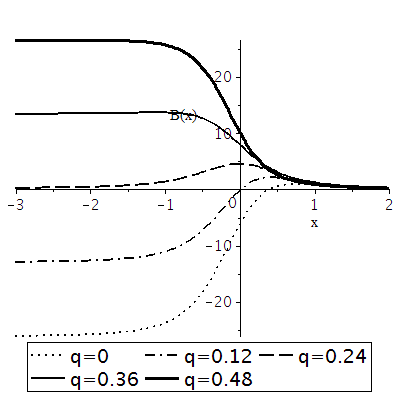
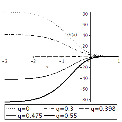
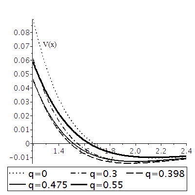
a                                                 b                                                 c

Figure 2: The function $B(x)$ (a) and the potential $V(x)$ (b, c) for some asymmetric configurations with $0\leq q<1$. Panel c shows the behavior of $V$ at comparatively large $x$ invisible in panel b.

At the other extreme, $x\to-\infty$, possible values $B(-\infty)<0$ correspond to de Sitter asymptotic behavior (dS), and, since it is a T-region, it is an expanding or contracting cosmology, in other words, we obtain a black universe.

If $B(-\infty)=0$, which happens if $p=0$, the metric is asymptotically flat, and the whole solution is symmetric with respect to the surface $x=0$ since both $B(x)$ and $r(x)$, as well as the potential $V(x)$ are even functions. In this case, the mass and charge are related by $m=(2/3)\pi q^{2}$.

Lastly, we obtain an anti-de Sitter (AdS) asymptotic if $B(-\infty)>0$. The resulting solutions can be classified according to the asymptotic behaviors at the two infinities and the number and kind of horizons that correspond to zeros of $B(x)$.

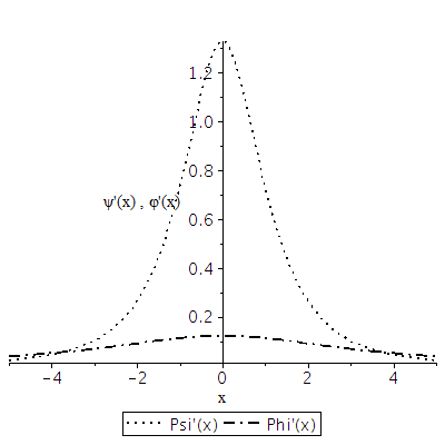
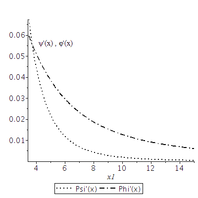
Figure 3: The quantities $\phi^{\prime}$ and $\psi^{\prime}$ in the strong and weak field regions

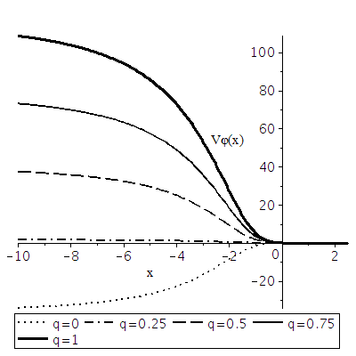
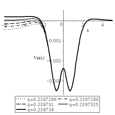
Figure 4: The potential $V_{\phi}(x)$ for $m=1/2$ and some values of the charge $q$. The right panel demonstrates the detailed behavior of $V_{\phi}(x)$ close to the critical value $q=q_{0}=0.238673$, at which the number of its zeros changes. There is a very narrow range of $q$, $q_{0}<q<0.238733$, where $V_{\phi}(x)$ has two zeros at negative values of $x$.

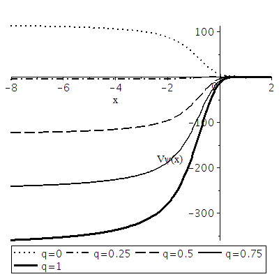
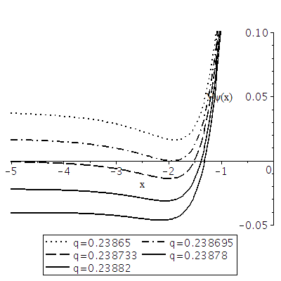
Figure 5: The potential $V_{\psi}$ for $m=1/2$ and the same values of $q$ as in Fig. 4. The right panel shows the behavior of $V_{\psi}(x)$ at $q$ close to $q_{0}$.

The possible kinds of geometries obtained have the same qualitative features as those discussed in [12, 11], so we will not describe them here in full detail. In particular, we refer to [12] for a description of the corresponding global causal structures and Carter-Penrose diagrams, which (since $r(x)\approx|x|$ at both infinities) are completely determined by the zeros of $B(x)$ and the signs of its asymptotic values.

In the case of symmetric, twice asymptotically flat solutions we have the following types of geometries (see Fig. 1): (i) a wormhole ($0\leq|q|\lesssim 0.398$), (ii) an extremal regular black hole with a single horizon $(q\approx 0.398)$, and (iii) a non-extremal regular black hole with two simple horizons $(q\gtrsim 0.398)$ (Fig. 1). It is of interest that small changes of $q$ near the critical value $\approx 0.398$ drastically change $B(x)$ whereas the function $V(x)$ changes very little. One can also note that at large $|x|$ the potential $V(x)$ has small negative values (Fig. 1c) while it is comparatively large and positive at small $x$.

Asymmetric configurations, asymptotically flat at $x=\infty$, are slightly more diverse. Fig. 2 shows some of them under the assumption $m=1$ adopted for definiteness. Note that in both figures 1a and 2a all curves $B(x)$ approach $x=\infty$ from positive since there is an R-region and Schwarzschild asymptotic.

For the scalar field $\phi$, by analogy with [11], we assume the form

$$\phi(x)=K\arctan(Lx),$$ (21)

where $K$ and $L$ are adjustable constants. By (21) and (10),

$${}\phi^{\prime 2}(x)=\frac{K^{2}L^{2}}{(L^{2}x^{2}+1)^{2}},$$ (22)

$${}\psi^{\prime 2}(x)=\frac{28-2x^{2}}{(x^{2}+1)(x^{2}+4)^{2}}+\frac{K^{2}L^{2}}{(L^{2}x^{2}+1)^{2}}.$$ (23)

Let us choose $K$ and $L$ in such a way as to make the phantom field $\psi$ decay at large $x$ more rapidly than $\phi$. From (23) we have

$$\psi^{\prime 2}(x)=\frac{K^{2}-2L^{2}}{L^{2}x^{4}}+\frac{46L^{4}-2K^{2}}{L^{4}x^{6}}+O(x^{-8}),$$ (24)

hence taking

$$K=2/\sqrt{23},\quad\ L=\sqrt{2/23},$$ (25)

we obtain $\psi^{\prime}\sim x^{-4}$ whereas $\phi^{\prime}\sim x^{-2}$ at large $|x|$, as required. We use the values (25) in our numerical calculations. The behavior of $\phi^{\prime}(x)$ and $\psi^{\prime}(x)$ is shown in Fig. 3.

The field potential $V_{\phi}(x)$ is found from Eq. (12) under the boundary condition $V_{\phi}(\infty)=0$. The other potential $V_{\psi}$ is obtained as

$$V_{\psi}=V-V_{\phi},$$ (26)

or it can be equivalently found from Eq. (13). The expressions for the potentials are found analytically but are too bulky to be presented here, so we only show their plots for some values (Figs. 4 and 5), again putting $m=1$. Other values of $m$ do not add any new qualitative features of the solution.

Summarizing, we have obtained examples of wormhole, regular black hole and black universe solutions to the field equations with two scalars $\phi$ (canonical) and $\psi$ (phantom), in which the phantom field comparatively quickly decays at infinity.

Appendix: linear perturbations

Consider an action with a single scalar field, but more general than (2) in that we admit a dilatonic-type interaction between the scalar and electromagnetic fields:

$${}{\cal S}=\frac{1}{16\pi}\int\sqrt{-g}d^{4}x\Big{[}R+2h(\phi)g^{\alpha\beta}\phi_{;\alpha}\phi_{;\beta}$$

$${}\ \ -2V(\phi)-S(\phi)F_{\mu\nu}F^{\mu\nu}\Big{]},$$ (A1)

where $h>0$ for a normal scalar field with positive kinetic energy and $h<0$ for a phantom one; the function $S(\phi)>0$, characterizing the scalar-electromagnetic interaction, is arbitrary. The field equations are

$$4h\nabla^{\mu}\nabla_{\mu}\phi+\eta S_{\phi}F_{\mu\nu}F^{\mu\nu} = 0,$$ (A2)

$$\nabla_{\mu}(S(\phi)F^{\mu\nu}) = 0,$$ (A3)

$$R_{\mu}^{\nu}-{{\textstyle\frac{1}{2}}}\delta_{\mu}^{\nu}R = -T_{\mu}^{\nu},$$ (A4)

where $S_{\phi}\equiv dS/d\phi$ and $T_{\mu}^{\nu}$ is the SET:

$${}T_{\mu}^{\nu}=T_{\mu}^{\nu}[\phi]+T_{\mu}^{\nu}[F],$$

$${}T_{\mu}^{\nu}[\phi]=h(\phi)[2\phi_{\mu}\phi^{\nu}-\delta_{\mu}^{\nu}\phi^{\alpha}\phi_{\alpha}]+\delta_{\mu}^{\nu}V(\phi),$$

$${}T_{\mu}^{\nu}[F]=S(\phi)\big{[}-2F_{\mu\alpha}F^{\nu\alpha}+{{\textstyle\frac{1}{2}}}\delta_{\mu}^{\nu}F_{\alpha\beta}F^{\alpha\beta}].$$ (A5)

The general static, spherically symmetric metric may be written in the form

$$ds^{2}={\,\rm e}^{2\gamma}dt^{2}-{\,\rm e}^{2\alpha}du^{2}-{\,\rm e}^{2\beta}d\Omega^{2},$$ (A6)

where $\gamma$, $\alpha$ and $\beta$ are functions of the radial coordinate $u$. There remains a coordinate freedom of choosing $u$. We also use the notation $r(u)\equiv{\,\rm e}^{\beta}$.

We are going to study linear spherically symmetric perturbations of solutions to the field equations due to (Appendix: linear perturbations). So, the metric has the form (A6) but now $\gamma(u,t)=\gamma(u)+\delta\gamma$ and similarly for other quantities, with small “deltas”; for the scalar field we have $\phi(u,t)=\phi(u)+\delta\phi(u,t)$. The most general electromagnetic field compatible with spherical symmetry is described by the 4-potential

$$A_{\mu}=\delta_{\mu}^{0}A_{0}+\delta_{\mu}^{3}q_{m}\cos\theta+\partial_{\mu}\Phi,$$ (A7)

where $q_{m}$ is a magnetic charge and $\Phi$ an arbitrary function. The electromagnetic field equations give

$$S(\phi){\,\rm e}^{\alpha+2\beta+\gamma}F^{10}=q_{e},$$ (A8)

where $q_{e}$ is an electric charge. We thus have

$$F_{\mu\nu}F^{\mu\nu}=2{\,\rm e}^{-4\beta}(-q_{e}^{2}/S^{2}+q_{m}^{2}).$$ (A9)

For the SETs we obtain

$$T_{\mu}^{\nu}[\phi] = \varepsilon{\,\rm e}^{-2\alpha}\phi^{\prime 2}\mathop{\rm diag}\nolimits(1,\ -1,\ 1,\ 1)+\delta_{\mu}^{\nu}V,$$ (A10)

$$T_{\mu}^{\nu}[F] = \eta{\,\rm e}^{-4\beta}Q(\phi)\mathop{\rm diag}\nolimits(1,\ 1,\ -1,\ -1).$$ (A11)

where $Q=Q(\phi)=q_{e}^{2}/S(\phi)+q_{m}^{2}S(\phi)$. We will consider the equations governing linear radial perturbations of a static, spherically symmetric solution to the field equations (A2)–(A4), following the lines of [3, 16, 17, 18].

Preserving only linear terms with respect to time derivatives, we can write all nonzero components of the Ricci tensor as

$$R^{0}_{0} = {\,\rm e}^{-2\gamma}(\ddot{\alpha}+2\ddot{\beta})$$ (A12)

$${}\ \ \ -{\,\rm e}^{-2\alpha}[\gamma^{\prime\prime}+\gamma^{\prime}(\gamma^{\prime}-\alpha^{\prime}+2\beta^{\prime})],$$

$${}R^{1}_{1} = {\,\rm e}^{-2\gamma}\ddot{\alpha}-{\,\rm e}^{-2\alpha}[\gamma^{\prime\prime}+2\beta^{\prime\prime}+\gamma^{\prime}{}^{2}$$ (A13)

$${}\ \ \ +2\beta^{\prime}{}^{2}-\alpha^{\prime}(\gamma^{\prime}+2\beta^{\prime})],$$

$${}R^{2}_{2} = R^{3}_{3}={\,\rm e}^{-2\beta}+{\,\rm e}^{-2\gamma}\ddot{\beta}$$ (A14)

$${}\ \ \ -{\,\rm e}^{-2\alpha}[\beta^{\prime\prime}+\beta^{\prime}(\gamma^{\prime}-\alpha^{\prime}+2\beta^{\prime})],$$

$${}R_{01} = 2[\dot{\beta}^{\prime}+\dot{\beta}\beta^{\prime}-\dot{\alpha}\beta^{\prime}-\dot{\beta}\gamma^{\prime}],$$ (A15)

where dots and primes denote $\partial/\partial t$ and $\partial/\partial u$, respectively.

The zero-order (static) scalar, ${0\choose 0}$, ${1\choose 1}$, ${2\choose 2}$ components of Eqs. (A4) are

$${}2h[\phi^{\prime\prime}+\phi^{\prime}(\gamma^{\prime}+2\beta^{\prime}-\alpha^{\prime})]+h^{\prime}\phi^{\prime}={\,\rm e}^{2\alpha}P_{\phi};$$ (A16)

$${}\gamma^{\prime\prime}+\gamma^{\prime}(\gamma^{\prime}+2\beta^{\prime}-\alpha^{\prime})={\,\rm e}^{2\alpha}(-V+Q{\,\rm e}^{-4\beta});$$ (A17)

$${}\gamma^{\prime\prime}+2\beta^{\prime\prime}+\gamma^{\prime}{}^{2}+2\beta^{\prime}{}^{2}-\alpha^{\prime}(\gamma^{\prime}+2\beta^{\prime})$$

$${}\ \ =-2h\phi^{\prime 2}+{\,\rm e}^{2\alpha}(-V+Q{\,\rm e}^{-4\beta});$$ (A18)

$${}-{\,\rm e}^{2\alpha-2\beta}+\beta^{\prime\prime}+\beta^{\prime}(\gamma^{\prime}+2\beta^{\prime}-\alpha^{\prime})=-P{\,\rm e}^{2\alpha},$$ (A19)

where the subscript $\phi$ denotes $\partial/\partial\phi$ and

$$P:=V(\phi)+Q{\,\rm e}^{-4\beta},$$ (A20)

The first-order perturbed equations (scalar, $R_{01}=\ldots$, and $R^{2}_{2}=\ldots$) read

$${}2{\,\rm e}^{2\alpha-2\gamma}h\delta\ddot{\phi}-2h[\delta\phi^{\prime\prime}$$

$${}\ +\delta\phi^{\prime}(\gamma^{\prime}+2\beta^{\prime}-\alpha^{\prime})+\phi^{\prime}(\delta\gamma^{\prime}+2\delta\beta^{\prime}-\delta\alpha^{\prime})]$$

$${}\ -2\delta h[\phi^{\prime\prime}+\phi^{\prime}(2\beta^{\prime}+\gamma^{\prime}-\alpha^{\prime})]$$

$${}\ -h^{\prime}\delta\phi^{\prime}-\phi^{\prime}\delta h^{\prime}+\delta({\,\rm e}^{2\alpha}P_{\phi})=0,$$ (A21)

$${}\delta\dot{\beta}^{\prime}+\beta^{\prime}\delta\dot{\beta}-\beta^{\prime}\delta\dot{\alpha}-\gamma^{\prime}\delta\dot{\beta}=-h\phi^{\prime}\delta\dot{\phi},$$ (A22)

$${}\delta({\,\rm e}^{2\alpha-2\beta})+{\,\rm e}^{2\alpha-2\gamma}\delta\ddot{\beta}-\delta\beta^{\prime\prime}-\delta\beta^{\prime}(\gamma^{\prime}+2\beta^{\prime}-\alpha^{\prime})$$

$${}\qquad-\beta^{\prime}(\delta\gamma^{\prime}+2\delta\beta^{\prime}-\delta\alpha^{\prime})=\delta({\,\rm e}^{2\alpha}P),$$ (A23)

Eq. (A22) may be integrated in $t$; since we are interested in time-dependent perturbations, we omit the appearing arbitrary function of $u$ describing static perturbations and obtain

$$\delta\beta^{\prime}+\delta\beta(\beta^{\prime}-\gamma^{\prime})-\beta^{\prime}\delta\alpha=-h\phi^{\prime}\delta\phi.$$ (A24)

Let us note that we have two independent forms of arbitrariness: one is the freedom of choosing a radial coordinate $u$, the other is a perturbation gauge, or, in other words, a reference frame in the perturbed space-time, which can be expressed in imposing a certain relation for $\delta\alpha,\ \delta\beta$, etc. In what follows we will employ both kinds of freedom. All the above equations have been written in the most universal form, without coordinate or gauge fixing.

Preserving the coordinate arbitrariness, we will now choose the simplest possible gauge $\delta\beta\equiv 0$. Then Eq. (A24) expresses $\delta\alpha$ in terms of $\delta\phi$:

$$\beta^{\prime}\delta\alpha=h(\phi)\phi^{\prime}\delta\phi.$$ (A25)

Eq. (Appendix: linear perturbations) expresses $\delta\gamma^{\prime}-\delta\alpha^{\prime}$ in terms of $\delta\alpha$ and $\delta\phi$:

$$\beta^{\prime}(\delta\gamma^{\prime}-\delta\alpha^{\prime})=2{\,\rm e}^{2\alpha-2\beta}\delta\alpha-\delta({\,\rm e}^{2\alpha}P).$$ (A26)

Substituting all this into (Appendix: linear perturbations), we finally obtain the following wave equation:

$${}{\,\rm e}^{2\alpha-2\gamma}\delta\ddot{\phi}-\delta\phi^{\prime\prime}-\delta\phi^{\prime}(\gamma^{\prime}+2\beta^{\prime}-\alpha^{\prime}+h^{\prime}/h)$$

$${}\hskip 72.26999pt+U\delta\phi=0,$$ (A27)

$${}U\equiv{{\displaystyle\frac{1}{2}}}\phi^{\prime}{}^{2}\biggl{(}\frac{h_{\phi}^{2}}{h^{2}}-\frac{h_{\phi\phi}}{h}\biggr{)}+{\,\rm e}^{2\alpha}\biggl{[}\frac{2h\phi^{\prime 2}}{\beta^{\prime 2}}(P-{\,\rm e}^{-2\beta})$$

$${}\hskip 28.45274pt\hskip 28.45274pt+\frac{2\phi^{\prime}}{\beta^{\prime}}P_{\phi}+\frac{h_{\phi}}{2h^{2}}P_{\phi}-\frac{P_{\phi\phi}}{2h}\biggr{]}.$$ (A28)

This expression for $U$ directly generalizes the one obtained in [18] for scalar-vacuum configurations. The latter is restored if we assume $h=\epsilon=\pm 1$ and $q_{e}=q_{m}=0$.

Passing on to the “tortoise” coordinate $x$ introduced according to

$$du/dx={\,\rm e}^{\gamma-\alpha}$$ (A29)

and changing the unknown function $\delta\phi\mapsto\psi$ according to

$$\delta\phi=\psi(x,t){\,\rm e}^{-\eta},\hskip 28.45274pt\eta^{\prime}=\beta^{\prime}+\frac{h^{\prime}}{2h},$$ (A30)

we reduce the wave equation to its canonical form, also called the master equation for radial perturbations:

$$\ddot{\psi}-\psi_{xx}+V_{\rm eff}(x)\psi=0,$$ (A31)

(the index $x$ denotes $d/dx$), with the effective potential

$${}V_{\rm eff}(x)={\,\rm e}^{2\gamma-2\alpha}[U+\eta^{\prime\prime}+\eta^{\prime}(\eta^{\prime}+\gamma^{\prime}-\alpha^{\prime})].$$ (A32)

A further substitution

$$\psi(x,t)=y(x){\,\rm e}^{i\omega t},\hskip 28.45274pt\omega={\rm const},$$ (A33)

which is possible because the background is static, leads to the Schrödinger-like equation

$$y_{xx}+[\omega^{2}-V_{\rm eff}(x)]y=0.$$ (A34)

If there is a nontrivial solution to (A34) with $\mathop{\rm Im}\nolimits\omega<0$ satisfying some physically reasonable conditions at the ends of the range of $u$ (in particular, the absence of ingoing waves), then the static system is unstable since $\delta\phi$ can exponentially grow with $t$. Otherwise our static system is stable in the linear approximation. Thus, as usual in such studies, the stability problem is reduced to a boundary-value problem for Eq. (A34) — see, e.g., [3, 16, 17, 18, 19, 20, 21, 22, 23, 24].

Note that all the above relations are written without fixing the background radial coordinate $u$.

The gauge $\delta\beta=0$ is technically the simplest one, but causes certain problems when applied to wormholes and other configurations with throats. The reason is that the assumption $\delta\beta=0$ leaves invariable the throat radius, while perturbation must in general admit its time dependence [19, 22, 3]. It may even seem that the emergence of a pole in $V_{\rm eff}$ due to $\delta\beta$ in the denominator in (Appendix: linear perturbations) is an artefact of the gauge. It turns out, however, that, by analogy with [22, 18, 3], Eq. (A34) is in fact gauge-invariant, while $\delta\phi$ is a representation of a gauge-invariant quantity in the gauge $\delta\beta=0$.

Therefore, singularities of the effective potential $V_{\rm eff}$ are of objective nature. The singularity at $\beta^{\prime}=0$ (e.g., a throat) can be regularized [22, 18], and moreover, it can be shown that regular solutions to the regularized equations describe regular perturbations of both the scalar field and the metric. It was this procedure that made it possible to prove the instability of anti-Fisher (Ellis type [25, 26]) wormholes [22] and other scalar field configurations in general relativity [18, 23].

The effective potential $V_{\rm eff}$ also possesses singularities at the values of the radial coordinate where $h=0$, which exist in the cases where the function $h(\phi)$ in (Appendix: linear perturbations) changes its sign. This happens in the framework of the trapped ghost concept. The existing experience [16, 17, 22, 18, 23] shows that such singularities are in general an indication of instabilities, even if $V_{\rm eff}\to\infty$ at such a singularity. As already mentioned, this was one of the reasons for our attempt to replace a “trapped ghost” in wormhole and black universe models with an “invisible” one.

References

- [1] P. A. R. Ade et al. (Planck Collaboration), “Planck 2015 results. XIII. Cosmological parameters”, ArXiv: 1502.01589.
- [2] M. Visser, Lorentzian Wormholes: from Einstein to Hawking (AIP, Woodbury, 1995).
- [3] K. A. Bronnikov and S. G. Rubin, Black Holes, Cosmology and Extra Dimansions (World Scientific, Singapore, 2012).
- [4] Francisco S. N. Lobo, “Time machines and traversable wormholes in modified theories of gravity”, EPJ Web Conf. 58, 01006 (2013), ArXiv: 1212.1006.
- [5] K. A. Bronnikov and M. V. Skvortsova, “Cylindrically and Axially Symmetric Wormholes. Throats in Vacuum?”, Grav. Cosmol. 20, 171–175 (2014); ArXiv: 1404.5750.
- [6] D. Hochberg and M. Visser, Phys. Rev. D 56, 4745 (1997); gr-qc/9704082.
- [7] K. A. Bronnikov and J. C. Fabris, “Regular phantom black holes”, Phys. Rev. Lett. 96, 251101 (2006); gr-qc/0511109.
- [8] K. A. Bronnikov, V. N. Melnikov and H. Dehnen, “Regular black holes and black universes”, Gen. Rel. Grav. 39, 973 (2007); gr-qc/0611022.
- [9] K. A. Bronnikov and S. V. Sushkov, “Trapped ghosts: a new class of wormholes”, Class. Quantum Grav. 27, 095022 (2010); ArXiv: 1001.3511.
- [10] K. A. Bronnikov and E. V. Donskoy, “Black universes with trapped ghosts”, Grav. Cosmol. 17, 176 (2011); ArXiv: 1110.6030.
- [11] K. A. Bronnikov, E. V. Donskoy and P. A. Korolev, “Magnetic wormholes and black universes with trapped ghosts”, Vestnik RUDN No. 2, 139–149 (2013).
- [12] S. V. Bolokhov, K. A. Bronnikov, and M. V. Skvortsova, “Magnetic black universes and wormholes with a phantom scalar”, Class. Quantum Grav. 29,, 245006 (2012); ArXiv: 1208.4619.
- [13] J. A. Wheeler, “Geons”, Phys. Rev. 97, 511 (1955).
- [14] R. Poltis and D. Stojkovic, “Can primordial magnetic fields seeded by electroweak strings cause an alignment of quasar axes on cosmological scales?”, Phys. Rev. Lett. 105, 161301 (2010); arXiv: 1004.2704.
- [15] M. S. Morris and K. S. Thorne, “Wormholes in space-time and their use for interstellar travel: a tool for teaching General Relativity”, Am. J. Phys. 56, 395 (1988).
- [16] K. A. Bronnikov and A. V. Khodunov, “Scalar field and gravitational instability”, Gen. Rel. Grav. 11, 13 (1979).
- [17] K. A. Bronnikov and Yu. N. Kireyev, “Instability of black holes with scalar charge”, Phys. Lett. A 67, 95 (1978).
- [18] K. A. Bronnikov, J. C. Fabris, and A. Zhidenko, “On the stability of scalar-vacuum space-times”, Euro Phys. J. C 71, 1791 (2011); Arxiv: 1109.6576.
- [19] K. A. Bronnikov, C. P. Constantinidis, R. Evangelista, and J. C. Fabris, “Electrically charged cold black holes in scalar-tensor theory”, Int. J. Mod. Phys. D 8, 481 (1999); gr-qc/9903028.
- [20] K. A. Bronnikov and S. V. Grinyok, “Conformal continuations and wormhole instability in scalar-tensor gravity”, Grav. Cosmol. 10, 237 (2004); gr-qc/0411063.
- [21] K. A. Bronnikov and S. V. Grinyok, “Electrically charged and neutral wormhole instability in scalar-tensor gravity”, Grav. Cosmol. 11, 75 (2005); gr-qc/0509062.
- [22] J. A. Gonzalez, F. S. Guzman, and O. Sarbach, “Instability of wormholes supported by a ghost scalar field. I. Linear stability analysis”, Class. Quantum Grav. 26,, 015010 (2009); Arxiv: 0806.0608.
- [23] K. A. Bronnikov, R. A. Konoplya, and A. Zhidenko, “Instability of wormholes and regular black holes supported by a phantom scalar field”, Phys. Rev. D 86,, 024028 (2012); ArXiv: 1205.2224.
- [24] K. A. Bronnikov, L. N. Lipatova, I. D. Novikov, and A. A. Shatskiy, “Example of a stable wormhole in general relativity”, Grav. Cosmol. 19, 269 (2013).
- [25] K. A. Bronnikov, “Scalar-tensor theory and scalar charge”, Acta Phys. Pol. B4, 251 (1973).
- [26] H. Ellis, “Ether flow through a drainhole: A particle model in general relativity”, J. Math. Phys. 14, 104 (1973).