Abstract

Abstract

Recently, HTTP-Based Adaptive Streaming has become the de facto standard for video streaming over the Internet. It allows the client to dynamically adapt media characteristics to varying network conditions in order to maximize Quality of Experience, that is, minimize playback interruptions, while maximizing video quality at a reasonable level of quality changes. In the case of live streaming, where buffering possibilities are limited, this task becomes particularly challenging. An important factor than might help improving performance is the capability to correctly predict network throughput dynamics on short to medium timescales. This problem becomes notably difficult in wireless networks that are often subject to continuous throughput fluctuations.

In the present work, we develop an adaptation algorithm for HTTP-Based Adaptive Live Streaming that, for each adaptation decision, maximizes a Quality of Experience based utility function depending on the probability of playback interruptions, average video quality, and the amount of video quality fluctuations. To compute the utility function, in particular the interruption probability, the algorithm leverages throughput predictions, and dynamically estimated prediction accuracy.

We are trying to close the gap created by the lack of studies analyzing TCP throughput on short to medium timescales. We study several time series prediction methods and model the distribution of prediction errors. We observe that Simple Moving Average, despite being the most straightforward method, performs best in most cases. We also observe that the relative underestimation error is best represented by a truncated normal distribution, while the relative overestimation error is best represented by a Lomax distribution. Moreover, although underestimations and overestimations are balanced in all traces, they exhibit a strong temporal correlation that we use to further improve prediction accuracy.

We compare the proposed algorithm with a baseline approach that uses a fixed margin between past throughput and selected media bit rate, and an oracle-based approach that has perfect knowledge of future throughput for a certain time horizon.

Chapter 0 Introduction

Over the last years, we have been observing a dramatic change in video consumption patterns. The era of passive consumption of non-interactive "linear" content on a single device that does not offer much functionality is clearly over. Enabled by advances in media compression technologies, miniaturization and increasing processing power of electronic devices, complemented by ubiquitous availability of broadband access networks, we are witnessing the establishment of a new mindset: watch what I want, when I want, and where I want. A multitude of devices is at user’s command to gain access to a vast sea of video content at any time and location: smartphones, tablets, PC’s, game consoles, and, of course, TV sets that, however, underwent a transformation to become what is called Hybrid TV’s, connected to the Internet and offering a multitude of interactive applications. [6, 8] Moreover, as wearable devices such as smart watches and Google Glass begin to gain popularity, they might take the digital media landscape to a whole new level. All these devices empower the user to watch their favorite content on the best screen available at that moment, and not at the behest of the content provider.

Another game changer has been the advance of Web 2.0 [32], that has expanded the focus of Internet from publishing to participation, allowing anyone to publish to the world without having to go through the closed systems that have dominated media since its very beginning. The plethora of freely accessible User-Generated Content (UGC), shared over Social Networking Services, boosted the demand for watching video over the Internet and brought online video into the mainstream. As of today, the number of UGC objects is orders of magnitude higher than that of traditional movies or TV programs and is rapidly evolving [26]. One prominent example reflecting this development is YouTube that alone reaches more US adults at the age of 18-34 than any cable network. As of January 2015, over 6 billion hours of video are watched each month on YouTube, which is almost an hour for every person on Earth. 100 hours of video are uploaded to YouTube every minute [9]. And: around 25.0% of the daily views on YouTube come from person-to-person sharing [13].

This development is being accompanied by a shift towards usage of wireless and mobile networks. In 2013, wired devices still accounted for the majority of Internet traffic at 56%. The status quo, however, is rapidly changing. Traffic from wireless and mobile devices is predicted to exceed traffic from wired devices by 2018, accounting for 61% of the total Internet traffic. And by far the largest part of it is video. Globally, video traffic is estimated to be 79% of all consumer Internet traffic in 2018, up from 66% in 2013 [5]. The majority of streamed content is Video on Demand (VoD). However, the amount of live streaming, such as of sports events, video gaming, or music concerts, is experiencing rapid growth, promising significant revenues to the stakeholders [42].

This enormous amount of traffic places a huge burden on the Internet infrastructure and on state-of-the-art wireless and mobile networks, and requires novel efficient solutions both in the area of wireless and mobile networking and video streaming. While a classical broadcaster exclusively uses a channel to broadcast to everyone within reach, on the Internet, the medium is shared among many users and a separate, unicast data stream is transmitted to every single receiver. Recent studies suggest that the challenges have not yet been successfully addressed. In 2013, around 26.9% of streaming sessions on the Internet experienced playback interruption due to rebuffering, 43.3% were impacted by low resolution, and 4.8% failed to start altogether. [7]

One of the problems is the Internet was not designed to support applications that require configurable end-to-end Quality of Service (QoS) [2]. Considerable effort has been put into developing networking architectures, addressing this shortcoming [10, 14]. So far, none of them achieved a significant pervasiveness. Especially on wireless and mobile links, a user is exposed to interference, cross-traffic, and fading effects, leading to continuously fluctuating QoS characteristics. As a consequence, we lately have been observing a thriving period for adaptive streaming technologies that are able to dynamically adjust the characteristics of the streamed media to varying network conditions, leading to a smoother viewing experience with less playback interruptions and a more efficient utilization of available network resources.

In particular, one technology has become the de facto standard for Internet streaming: HTTP-Based Adaptive Streaming (HAS) [41]. Its advantage is that the usage of Hypertext Transfer Protocol (HTTP) allows to leverage the ubiquitous and highly optimized HTTP delivery infrastructure, including Content Delivery Networks, caches, proxies, etc. This allows to reduce costs due to maintenance of specialized video servers. Also, HTTP is usually allowed to traverse middleboxes, such as Network Address Translation (NAT) devices and firewalls. Of prime importance is also that HAS has good scalability properties due to the stateless nature of HTTP and because with HAS the control logic resides within the client. Thus, the server is relieved from keeping extensive state, and maintaining persistent feedback loops with the client. An open standard, MPEG-DASH (Dynamic Adaptive Streaming over HTTP) [4, 39], has been introduced to facilitate interoperability.

An important feature of HAS is that it uses Transmission Control Protocol (TCP) to transport the data, which has its pros and cons. On the one hand, TCP offers built-in congestion control and congestion avoidance mechanisms, that are necessary to maintain network stability, as well as to ensure basic fairness among competing flows. It also offers reliable communication by retransmitting lost packets, which enables usage of efficient video compression technologies that are particularly sensitive to packet losses. These features allow to reduce the complexity of the streaming application, which otherwise would have to implement mechanisms to deal with losses and congestion. [47] On the other hand, retransmissions delay subsequent packets, making TCP more challenging for live streaming. Further, TCP reacts to packet losses and transmission delay peaks by reducing its sending rate, which might negatively impact video quality.

The operation of HAS can be roughly described as follows. The video material is encoded in several representations, that vary w.r.t. their media characteristics such as spatial resolution, frame rate, compression level, etc. Typically, different representations have different media bit rates and thus different requirements on network throughput. Representations are split into segments, typically containing one to few seconds of video data. The data is encoded such that segments from different representations can be seamlessly played back after each other. The client issues a series of HTTP requests to download the segments in appropriate representations, trying to achieve certain goals.

For video streaming, identifying performance goals and expressing them in a way that facilitates objective measurement has turned out to be an extremely challenging task. One of the main reasons is that the ultimate target of a streaming service is a human being. Thus, an evaluation of such a service must inevitably take into account human perception and cognitive processing, involved in consuming the video content. These phenomena, however, are influenced by a large amount of hardly measurable factors. The notion of Quality of Experience (QoE) was introduced in an effort to assess these phenomena and help making them accessible to an objective evaluation process. The International Telecommunication Union (ITU) defines QoE as "the overall acceptability of an application or service, as perceived subjectively by the end-user", which might be influenced by "user expectations" and "context" [3]. The number of factors influencing QoE is immense, and many of them have a high level of subjectivity, which results in extremely complex modeling. [35]

With HAS, the degrees of freedom for maximizing QoE are determined by the choice of TCP as transport protocol on the one hand, and by putting the adaptation logic into the client, on the other. The media characteristics of available video representations are configured by the service provider during the planning phase. [37] The main factors influencing QoE that can be controlled by a HAS client are: initial delay, number and duration of rebuffering periods, selected video representation, and number and amplitude of representation changes. Their relative importance for QoE is, however, still poorly understood. Nevertheless, the number of studies dedicated to this topic has been dramatically increasing with the growing importance of video streaming, so that a lot of valuable insights are available to help designing QoE-optimized streaming mechanisms.

In particular, many studies suggest that the number and duration of rebuffering periods have the most severe impact on QoE, especially with live streaming. [7] In particular, users are willing to accept a higher initial delay and higher video distortion due to increased compression rate, if it helps minimizing rebuffering periods. [37, 17, 34, 38] On the other hand, it was observed that video quality fluctuations resulting from dynamically changing the representation can have a negative impact on QoE. [25, 46] In particular, some studies come to the conclusion that a lower overall video quality might be tolerated if it helps reducing the amount of representation changes. [33]

In the present study, we take up the position that a crucial factor influencing the ability of the client to maximize QoE, in particular, to minimize rebuffering, is his capability to correctly estimate network throughput dynamics on short to medium timescales. Specifically in the case of live streaming, where the time horizon for prefetching segments is limited and the time between the moment when a segment becomes available for download and its playback deadline typically constitutes few seconds, a client can strongly benefit from having a precise estimation of network throughput. This task is particularly challenging in wireless and mobile networks. It is further complicated by TCP’s congestion avoidance and control feedback loop, as well as retransmission mechanisms, contributing to the complexity of application-layer throughput dynamics.

Our contribution. In our work, we turn out attention to designing an adaptation algorithm for HTTP-Based Adaptive Live Streaming (HALS). Our idea is, prior to each segment download, to compare potential future adaptation trajectories and to select the one maximizing QoE. In order to evaluate QoE of an adaptation trajectory, we define a utility function depending on three factors that we call subutilities: (i) probability that a segment misses its playback deadline and thus the streaming session enters a rebuffering period, (ii) the distortion of video, evaluated by means of Peak Signal-to-Noise Ratio (PSNR), and (iii) the number and amplitude of representation changes. The utility is computed from individual subutilities in accordance with available literature on QoE. In particular, rebuffering subutility appears as a multiplicative factor and plays the role of an upper bound on the total utility, reflecting its strong impact on QoE. The other factor is a weighted sum of subutilities representing distortion and quality fluctuations that allows to resolve their trade-off in a configurable way.

In order to compute the defined utility, in particular, the probability that a segment misses its playback deadline, we study the predictability of TCP throughput in wireless networks over timescales from 1 to 10 seconds. For our study we use TCP throughput traces collected in IEEE 802.11bg Wireless Local Area Networks throughout Berlin, Germany, including public hotspots (indoor and outdoor), campus hotspots, and access points in residential environments. In particular, we focus on traces with low average throughput (hundreds of kilobits to few megabits per second), and high throughput fluctuations, which make the operation of a streaming client particularly challenging. We evaluate different time series prediction methods using varying numbers of past throughput measurements. We demonstrate that the most naïve method, Simple Moving Average (SMA) outperforms more sophisticated methods on all timescales, independent of the specific throughput dynamics. This means, somewhat surprisingly, that in studied environments, accounting for the trend in the past measurements does not help to increase prediction accuracy.

We further observe that prediction accuracy strongly varies across studied traces. Therefore, it is inefficient to assume a fixed prediction error and account for this error by a fixed margin between predicted throughput and selected media bit rate. On the contrary, it is crucial to dynamically estimate the prediction accuracy, in order to allow clients to efficiently utilize available network resources, at the same time being robust to throughput fluctuations. Consequently, we study approaches to model the prediction error and to estimate it for individual streaming sessions. We demonstrate that the overestimation error is extremely well represented by the Lomax distribution [22] on all considered timescales. The underestimation error is best represented by a truncated normal distribution except for the timescale of 1 second, where the truncated logistic distribution results in a slightly better Kolmogorov-Smirnov distance [16] between the empirical and the theoretical Cumulative Distribution Function (CDF). In addition, we find out that although underestimations and overestimations are balanced over the total duration of individual traces, they exhibit a strong temporal correlation that can be used to further improve prediction accuracy.

Armed with these insights we develop a novel adaptation algorithm for live streaming, which takes into account throughput predictions and an estimation of the relative prediction error, in order to maximize the defined QoE-related utility function. We evaluate the developed algorithm using collected throughput traces and show that it outperforms the baseline approach which uses a fixed margin.

In the following, Chapter 1 presents related work, Chapter 2 describes our system model, Chapter 3 details collected throughput traces, Chapter 4 studies throughput predictability and prediction accuracy, Chapter 5 presents the developed adaptation algorithm, Chapter 6 evaluates its performance, and Chapter 7 concludes the paper.

Chapter 1 Related work

There is a lack of studies systematically investigating approaches for TCP throughput prediction on short to medium timescales and evaluating their prediction accuracy. Consequently, only few works present adaptation algorithms that explicitly take into account throughput predictions. A common approach followed by many adaptive streaming clients is to use throughput averaged over a number of past measurements and one or multiple fixed safety margins to make adaptation decisions [30, 21, 27]. Other approaches leverage bandwidth probing techniques to obtain an estimation of network throughput [31], which, however, require support from the network infrastructure, server instrumentation, and/or modifying lower protocol layers.

Similar in spirit to our work is the rationale behind the adaptation algorithm proposed by Liu and Lee [29]. In contrast to their work, however, we first study statistical properties of prediction errors, which allows us to design an adaptation algorithm that uses a parametric approach, fitting the CDF of the prediction error to a distribution type determined during the preceding study. Proceeding this way requires significantly less data which allows the algorithm to operate without a database of measurements collected in the same environment. In addition, we separately model prediction errors on different timescales from 1 to 10 seconds. Moreover, we separately model underestimation and overestimation errors, which have quite different distributions, and their temporal correlation, which allows us to further improve prediction accuracy. Finally, instead of enforcing a minimum time between video quality adaptations, we are maximizing a utility function that includes a quality fluctuations related term, which is a more flexible approach, better suitable for live streaming, and allowing for a higher resource utilization.

Yin et al. [45] study the effect of prediction errors on performance of three adaptation approaches, buffer based, rate based, and Model Predictive Control (MPC). The study is using synthetic throughput traces and, due to the lack of literature on the subject, assumes that the prediction error has a normal distribution. In our study, we try to close this gap by evaluating several prediction methods and modeling the achievable prediction error on different timescales. Further, we develop an adaptation algorithm which takes into account the buffer level, throughput predictions on several timescales, and dynamically estimated prediction accuracy, and which specifically targets live streaming.

Tian and Liu [43] propose a prediction-based adaptation algorithm, where the media bit rate is selected to equal predicted throughput times dynamically varying adjustment factor. In contrast to this work, we predict throughput separately on different timescales, dynamically estimate prediction accuracy, and leverage temporal correlation of underestimations and overestimations. In addition, we select a video representation by maximizing a QoE-based utility function, depending on buffer underrun probability, video quality and video quality fluctuations.

Wang et al. [44] argue that for best performance, the mean media bit rate of streamed video should be roughly half the available network throughput. In our work we study throughput prediction accuracy in different environments, which enables us to develop an algorithm that dynamically tunes the margin between selected media bit rate and predicted throughput based on the buffer level and estimated prediction accuracy.

Jarnikov et al. [20] propose an adaptation algorithm based on a Markov decision process. With this approach, an optimal strategy is calculated offline for a given throughput distribution. We argue that assuming a fixed distribution, and neglecting temporal correlations, does not properly account for the variability of throughput dynamics in different environments.

Further improvement of an algorithm such as the one proposed in this work can potentially be achieved by complementing it with a data-driven, potentially location-based, approach operating as an outer loop on a macroscopic level [28, 36, 15].

A important research topic is QoE for adaptive video streaming [11, 37, 35, 40]. Rebuffering, initial delay, and quality fluctuations are factors that have not been part of traditional QoE metrics for video, but that have a tremendous impact on user’s perception of adaptive video streamed over a best-effort network, such as the Internet. User engagement is another important metric, which is especially of interest for content providers since it is directly related to advertising-based revenue schemes [12, 7].

Chapter 2 System model and notation

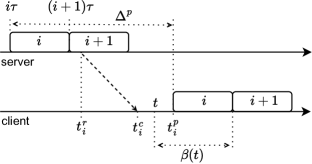
Figure 1: Illustration of client and server (event) timelines.

In the considered scenario a HAS client is live-streaming an event. The event to be streamed shall start at $t=0$. The stream is partitioned into segments. We denote the duration of video content contained in one segment by $\tau$. In order to simplify the presentation, we assume that all segments have equal duration. We use index $i\in\{1,2,\ldots,n\}$ to indicate a particular segment in a stream.

Segment $i$ shall contain video material covering the time period $\left[i\tau,\,(i+1)\tau\right]$, and become available for download at time $(i+1)\tau$. We assume that a segment must be completely downloaded prior to being processed by the client, and that the processing time at the client (that is, demultiplexing and decoding) is equal to 0, that is, the playback of a segment can start immediately after it has been completely downloaded. We argue that these fixed delays can be omitted without loss of generality. Using fixed non-zero delays would not affect the results but would make the notation more cumbersome.

Each segment is available in several representations. We denote the set of available representations by $\mathcal{R}$, indexed by $j\in\left\{1,2,\ldots,m\right\}$, with $m=\lvert\mathcal{R}\rvert$. W.l.o.g., $\mathcal{R}$ shall contain only representations feasible for the considered user. (A representation might be infeasible if its playback requires features not supported by the user or if its properties are excluded by configuration.)

We denote by $s_{ij}$ the size in bits, and by $\bar{r}_{ij}=s_{ij}/\tau$ the Mean Media Bit Rate (MMBR) of segment $i$ from representation $j$. We denote by $\bar{r}_{j}=1/n\sum_{i=1}^{n}{\bar{r}_{ij}}$ the MMBR of representation $j$. If the representation of a segment is clear from the context, we might omit index $j$. Thus, $s_{i}$ might, e.g., denote the size of a downloaded segment $i$, from the representation that was used to download it. Consequently, $\bar{r}_{i}=s_{i}/\tau$ then denotes the MMBR of segment $i$.

We use the following real-valued variables to denote continuous time in seconds. $t^{r}_{i}$ denotes the time when the request to download segment $i$ is sent by the user (at $t_{i}^{r}$, the client either just finished downloading the previous segment $i-1$, or segment $i$ just became available at the server). $t_{i}^{c}$ denotes the time when the last bit of segment $i$ is received by the user. $t_{i}^{p}$ denotes the time when the playback of segment $i$ is started. See Figure 1 for an illustration.

We denote the maximum playback delay by $\Delta^{p}_{\max}\geq 2\tau$, that is, playback of segment $i$ must not start later than $i\tau+\Delta^{p}_{\max}$. The lower bound of $2\tau$ stems from the fact that a segment can only be published $\tau$ seconds after its start, and that it takes, on average, up to further $\tau$ seconds to download it. Typical values for $\Delta^{p}_{\max}$ are assumed to be around 2 to 10 seconds. The actual playback delay, $\Delta^{p}\in\left[2\tau,\,\Delta^{p}_{\max}\right]$, is determined by the initial delay during the start of the streaming session and can be readjusted during each rebuffering event. The start of playback of segment $i$ is thus given by $t_{i}^{p}=i\tau+\Delta^{p}$. The value of $\Delta^{p}$ determines the maximum attainable buffer level, given by $\Delta^{p}-\tau$, and thus determines client’s sensitivity to throughput fluctuations and potential link outages. A client might dynamically tune $\Delta^{p}$ based on estimated throughput and link outage statistics. We leave that for future work and assume $\Delta^{p}=\Delta^{p}_{\max}$, maximizing the attainable buffer level, defined by

$$\beta(t)=\max\left\{t_{i}^{p}\;|\;t_{i}^{c}\leq t\right\}+\tau-t\,,$$

which is the time until all segments downloaded until time $t$ are played back, see Figure 1.

We denote by $\rho\left(t_{1},t_{2}\right)$ the mean application layer throughput in the time interval $\left[t_{1},t_{2}\right]$, that is, the number of bits received by the application from the TCP layer during this time interval, divided by $t_{2}-t_{1}$.

Chapter 3 TCP throughput traces

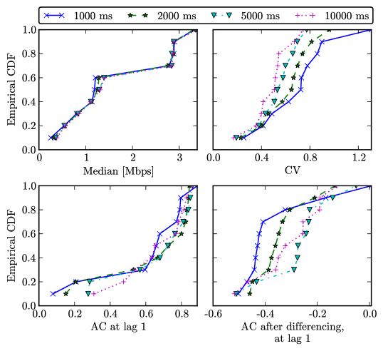
Figure 1: Application layer throughput statistics: median of the throughput, CV, auto-correlation at lag 1, and auto-correlation, after differencing, at lag 1. Lag 1 means here that the lag equals the size of the sampling interval.

For our study of TCP throughput prediction, as well as for performance evaluation of the developed adaptation algorithm, we recorded TCP throughput traces in IEEE 802.11bg networks at different locations throughout Berlin, Germany, including public hotspots (indoor and outdoor), campus hotspots, and access points in residential environments. The duration of the traces varies between 1500 and 1800 seconds each. The traces were collected using Lenovo ThinkPad L430 and T420 laptops, running Ubuntu 13.04 and Ubuntu 14.04 operating systems, with default Media Access Control (MAC) and TCP configurations.

From the set of collected traces we selected 10 that have a mean application-layer throughput between few hundreds of kilobit and few megabit per second. This throughput does not allow the client to select highest video representation, which we assume to be High-Definition (HD) video with an MMBR around 4 to 7 Mbps [23, 42]. In addition, the selected traces exhibit high throughput fluctuations that make low-delay live streaming particularly challenging.

From the traces, we generated time series containing incoming packets statistics, computed over sliding time intervals of 1 s to 10 s duration, shifted with a step size of 1 s. In addition to throughput statistics, our traces contain internal TCP and internal MAC information. The latter have been collected by putting the network interface into monitor mode and using radiotap headers [1]. TCP information includes delay jitter statistics and statistics of outstanding bytes. MAC information includes number of own frames received, number of other frames received, modulation scheme statistics, Signal Strength Indicator (SSI) statistics, and retransmission statistics.

To give a rough idea about properties of individual traces, Figure 1 presents basic throughput statistics. It shows median throughput, CV, auto-correlation at lag 1, and auto-correlation after differencing, at lag 1. Lag 1 means here that the lag equals the size of the averaging interval. The values are presented as Empirical Cumulative Distribution Functions, where each point in the graph corresponds to one trace. All traces can be downloaded from http://ns.tkn.tu-berlin.de/miller/. The software used to collect and process the data can be handed out upon request.

Chapter 4 Short-Term TCP throughput prediction

In this chapter, we present results on TCP throughput prediction for timescales from 1 to 10 seconds. Section 1 describes a selection of studied time series prediction methods, Section 2 presents evaluation results for three simple methods: SMA, linear extrapolation, and double exponential smoothing (Holt-Winters), and Section 3 presents modeling of the relative prediction error.

1 Prediction methods

We evaluated a number of time series prediction techniques, including SMA, linear extrapolation, Cubic Smoothing Splines (CSS), several flavors of exponential and double exponential smoothing, Autoregressive Integrated Moving Average (ARIMA), machine learning based methods, etc. A selection of studied methods is briefly described in the following. We abbreviate the methods by $\langle$type$\rangle$:$\langle n\rangle$:$\langle$parameters$\rangle$, where $\langle$type$\rangle$ is the name of the method, $n$ is the number of past measurements used as input, and $\langle$parameters$\rangle$ include further optional configuration parameters.

1 Simple moving average

SMA is probably the most simple prediction method imaginable. The predicted value is the average over a number of past measurements. The configuration parameters are: the number of past measurements, and the type of used mean value: arithmetic, geometric, or harmonic. In the following, we abbreviate this method with SMA:$\langle n\rangle$:$\langle$mean type$\rangle$, where $n\geq 1$ is the number of past measurements and type is one of $\{\text{ar},\text{gm},\text{hm}\}$. SMA:2:ar, e.g., means that the predicted value is the arithmetic mean from two past measurements. In particular, we denote the naïve approach of using the most recent measurement as predicted value with SMA:1:ar.

2 Simple exponential smoothing

With Simple Exponential Smoothing (SES), the predicted value is computed by averaging the past measurements, exponentially decreasing weights of older measurements. For given past measurements $x_{1},\ldots,x_{n}$, the predicted value is computed as $x_{n+1}=a_{n}$, with

$$a_{1} =x_{1}$$

$$a_{k} =\alpha x_{k}+(1-\alpha)a_{n-1}\,.$$

Besides the number of past measurements, it has a configuration parameter $\alpha\in\left[0,1\right]$. We tune $\alpha$ for each prediction by minimizing the Mean Squared Error (MSE) within past measurements, given by

$$\frac{1}{n-1}\sum_{k=2}^{n}{\left(x_{k}-a_{k-1}\right)^{2}}\,.$$

We abbreviate SES with SES:$\langle n\rangle$:mse, where $n\geq 2$ is the number of past measurements, and "mse" indicates the approach used to tune $\alpha$.

3 Linear extrapolation

Linear extrapolation is another straightforward prediction method that differs from SMA in that it takes into account the linear trend from past measurements. More specifically, linear extrapolation fits a linear curve into the set of given past measurements, minimizing the mean square error, and computes the prediction from extrapolating the curve to the prediction horizon. It thus requires at least two past measurements to compute a prediction. We abbreviate linear extrapolation with LinExt:$\langle n\rangle$, where $n\geq 2$ is the number of past measurements.

4 Double exponential smoothing

Similar to linear extrapolation, double exponential smoothing tries to account for the trend in the data, however, it assumes that most recent measurements have a higher significance for the prediction, and assigns older measurements exponentially decreasing weights. In the following, we use a variant of the method, sometimes called Holt-Winters double exponential smoothing. With Holt-Winters, for given past measurements $x_{1},\ldots,x_{n}$, the prediction is computed as $a_{n}+b_{n}$, where $a_{n},\;b_{n}$ are computed by the following recursive procedure.

$$a_{2} =x_{2}$$

$$b_{2} =x_{2}-x_{1}$$

$$a_{k} =\alpha x_{k}+(1-\alpha)(a_{k-1}+b_{k-1})\,,\;\text{for}\;k>2$$

$$b_{k} =\beta(a_{k}-a_{k-1})+(1-\beta)b_{k-1}\,,\;\text{for}\;k>2\,.$$

The Holt-Winters method has configuration parameters $\alpha$ and $\beta$ that dramatically influence the prediction quality and thus have to be carefully tuned. In our work we tune them for each prediction by minimizing the MSE within past measurements, which is given by

$$\frac{1}{n-2}\sum_{k=3}^{n}{\left(x_{k}-(a_{k-1}+b_{k-1})\right)^{2}}\,.$$

Thus, this method requires at least three past values for the prediction. As abbreviation we use HW:$\langle n\rangle$:mse, where $n\geq 3$ is the number of last values, and "mse" indicates the approach used to tune $\alpha$ and $\beta$.

5 Cubic smoothing splines

CSS model provides both smooth historical trend and a linear prediction function. The method uses a likelihood approach to estimate the smoothing parameter. It is based on finding piecewise cubic polynomials that are joined at the equally spaced time series points. [19]

6 Locally Weighted Scatterplot Smoothing (LOESS)

LOESS is a non-parametric regression method that tries to build a model describing the deterministic part of the variation in the data by incrementally fitting localized subsets of the data using simple regression models.

7 Autoregressive model

Autoregression model predicts the variable of interest by using a linear combination of past measurements, plus white noise. For past measurements $x_{1},\ldots,x_{n}$, the prediction of an autoregressive model of order $p$ can be written as:

$$x_{n+1}=c+\sum_{i=1}^{n}\alpha_{i}x_{i}+\omega_{n}\,,$$

where $c$ is a constant and $\omega_{n}$ denotes white noise. The order $p$ is selected by optimizing the Akaike Information Criterion (AIC).

8 Autoregressive Integrated Moving Average (ARIMA)

ARIMA is a combination of autoregressive and moving average models, with the ability to use a differenced or integrated representation of the time series. In our study, we were using a statistical method proposed in [18] that uses a combination of unit root test, minimization of the AIC and Maximum Likelihood Estimation (MLE) to reach an optimized ARIMA model.

2 Evaluation of prediction accuracy

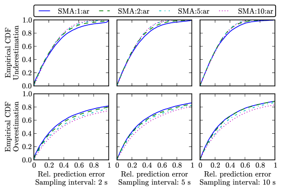
Figure 1: Relative prediction error for SMA on different timescales. (Higher values indicate higher prediction accuracy.) See Section 2 for details.

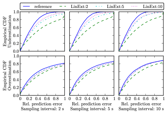
Figure 2: Relative prediction error for linear extrapolation on different timescales. (Higher values indicate higher prediction accuracy.) See Section 2 for details.

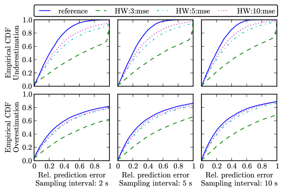
Figure 3: Relative prediction error for double exponential smoothing (Holt-Winters) on different timescales. (Higher values indicate higher prediction accuracy.) See Section 2 for details.

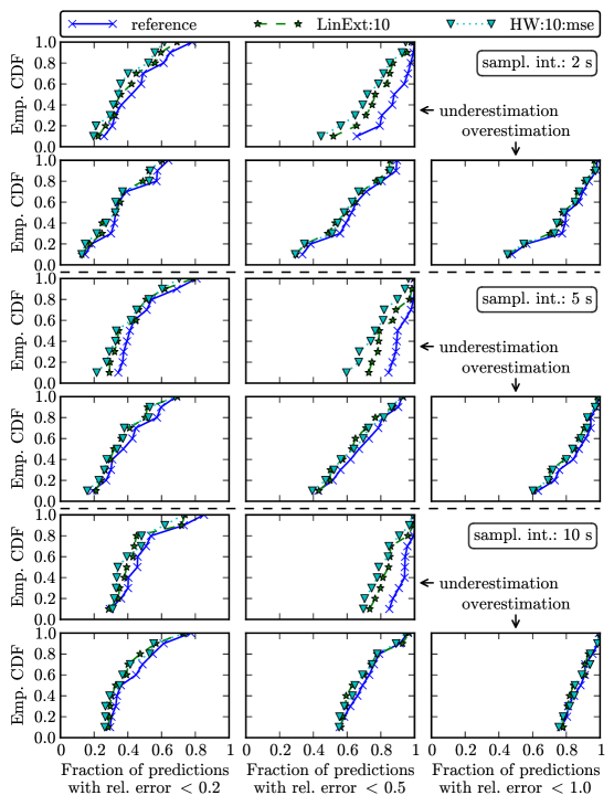
Figure 4: Quantiles of the relative prediction error for different prediction methods in individual traces. See Section 2 for details.

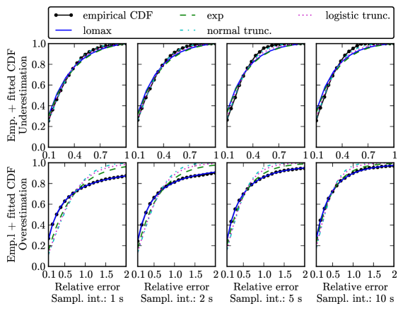
Figure 5: Fitting distributions for relative prediction errors. See Section 3 for details.

In order to evaluate the prediction accuracy, we use relative prediction error as metric, which we define as follows

$$\epsilon\left(t_{1},\,t_{2}\right)=\\ \frac{\lvert\max{\left(\hat{\rho}\left(t_{1},\,t_{2}\right),\,\rho_{\min}\right)}-\max{\left(\rho\left(t_{1},\,t_{2}\right),\,\rho_{\min}\right)}\rvert}{\max{\left(\rho\left(t_{1},\,t_{2}\right),\,\rho_{\min}\right)}}\,,$$ (1)

where $\hat{\rho}\left(t_{1},\,t_{2}\right)$ is a throughput prediction for the time interval $\left[t_{1},\,t_{2}\right]$. The maximum operator is necessary to avoid a distortion of results whenever $\rho\approx 0$ or $\hat{\rho}\leq 0$. We set $\rho_{\min}=10$ kbps.

We separately evaluate the overestimation and the underestimation error, due to the different error ranges of $(0,\infty)$ and $(0,1]$, respectively, and due to their different impact on the streaming client. An overestimation increases the risk of missing a playback deadline, resulting in a playback interruption, which has the strongest impact on QoE. An underestimation decreases the risk of interruptions but at the same time also reduces the media bit rate. In all studied traces, the relative frequency of underestimation and overestimation was close to 50% (see Section 4 for more details).

We made the, somewhat unexpected, observation that the increasing complexity of prediction methods such as ARIMA or machine learning based approaches does not improve prediction accuracy. Our conclusion was that accounting for the trend in the data does not help decreasing the prediction error. A potential explanation might be the negative auto-correlation of throughput time series after differencing, depicted in Figure 1. In particular, we observed that the median of the relative overestimation error of all studied methods is strictly greater than that of SMA:1:ar. Therefore, in the following, we present results focusing on three simple methods: SMA, linear extrapolation, and double exponential smoothing (Holt-Winters).

In the first step, we use for evaluation the complete set of measurements from all collected traces. The results are shown in Figures 1, 2, and 3. Figure 1 compares SMA using different numbers of past measurements, computed from non-overlapping time intervals. We observe that the overestimation error is smallest for SMA with only one past measurement, while the underestimation error improves when using more measurements. Consequently, in the following, we use SMA:1 as reference for the overestimation error and SMA:10 for the underestimation error. Figure 2 compares linear extrapolation with the respective reference method. We observe that two past measurements provide worst results, improving with the increasing number of past measurements but always remaining below the performance of SMA. Finally, Figure 3 compares Holt-Winters with SMA. Here, we observe the same situation as with linear extrapolation. It is also worth noting that Holt-Winters has a much higher computational complexity due to the optimization involved in tuning its configuration parameters for every new prediction.

Figure 4 shows results for individual traces. In order to present them in a compact way, this figure shows for each trace only three selected points of the ECDF, the fraction of measurements resulting in a relative error smaller than 0.2, 0.5, and 1.0, respectively. Each point on a subfigure corresponds to an individual trace so that the figures can be interpreted as ECDF’s over individual traces (where smaller values indicate higher prediction accuracy). The first two rows show results for a timescale of 2 seconds. The third and fourth rows for 5 seconds. The last two rows for 10 seconds. The first column shows for each trace the fraction of measurements with a relative error below 0.2, the second column below 0.5, and the last column below 1.0. The three missing subfigures are omitted since the relative error in the case of underestimation never exceeds $1.0$. To give an example, each point in the subfigure in the top row first column shows the fraction of underestimations in a particular trace with a relative error of less than 0.2. We observe that the per-trace comparison of prediction accuracy still indicates that in all cases, SMA performs better than the more sophisticated methods.

From Figures 1, 2, 3, and 4 we observe that with the reference method, a significant number of predictions result in a relatively small prediction error of below 20%. For example, in some traces, even on the timescale of 10 seconds, approximately 80% of predictions have an error smaller than 20%, while almost 100% of predictions have an error smaller than 50%. A relative error of this magnitude could, in principle, be accounted for by a fixed safety margin, that is, by always selecting a media bit rate which is by 20% smaller than the predicted throughput. There are, however, also "bad" traces, where more than 40% of overestimated predictions have a relative error of greater than 50%, while more than 20% of predictions still have an error greater than 100%, with even higher values for the timescale of 2 seconds.

Setting a high fixed safety margin to account for "bad" traces would result in significant underutilization of network resources, lower media bit rate and thus lower QoE in the "well-behaving" traces, while selecting a low fixed safety margin would increase the total re-buffering time in the "bad" traces, which, again, has a dramatic impact on QoE. Therefore, in the following section, we focus our attention on approaches to modeling and estimating the prediction error.

3 Error modeling

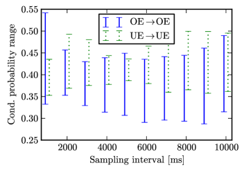
Figure 6: Conditional probability ranges (over traces) for underestimations (overestimations), given that previous prediction was an underestimation (overestimation).

In order to be able to use throughput predictions for adaptation decisions in the most efficient way, we turn out attention to modeling and estimating the relative prediction error. The approach we follow is to determine, which type of distributions fits well the ECDF of the prediction error. The developed adaptation algorithm for HALS, presented in Chapter 5 leverages the obtained results and estimates the parameters of this distribution for individual streaming sessions, or repeatedly throughout a streaming session.

We use the following distributions: exponential, normal, logistic, and Lomax (shifted Pareto) [22]. For the underestimation error, distributions are truncated to the range $[0,1]$, for the overestimation error to the range $[0,\infty)$. The CDF $F_{\text{tr}}(\cdot)$ of a distribution truncated to $[a,\,b]$ is obtained from the original CDF $F(\cdot)$ as

$$F_{\text{tr}}(x)=\frac{F(x)-F(a)}{F(b)-F(a)},\;\;x\in[a,\,b]\,.$$

We fit a distribution to the data by minimizing the squared distance ($L^{2}$-norm) between its CDF and the truncated ECDF. The ECDF is truncated in order to make the fit more precise in the range which is relevant for adaptive streaming clients. The ECDF of the overestimation error is truncated to the range $[0.1,2.0]$, in the case of underestimation to the range $[0.1,1.0]$. Afterwards, Kolmogorov-Smirnov test is used to verify the goodness of fit [16].

The results are shown in Figure 5. The CDF’s are fitted to ECDF’s over the joined set of measurements from all traces. It turns out that the overestimation error is extremely well represented by a Lomax distribution. The underestimation error is best represented by a truncated normal distribution except for the sampling interval of 1 second, where the truncated logistic distribution has a slightly better Kolmogorov-Smirnov distance. These findings are consistent with those obtained by fitting the prediction errors from individual traces, which are omitted here.

4 Underestimation and overestimation probabilities

Since underestimation and overestimation errors have different ranges, $\left[0,\,1\right]$, and $\left[0,\,\infty\right)$, and due to their different impact on the operation of a streaming client, we separately study the probabilities for underestimation and overestimation occurrence. In the following, we limit our presentation to SMA:1:ar.

In particular, we observed that in all studied traces the probability for occurrences of underestimations and overestimation are extremely well balanced on all timescales. Both occur in approximately $50\%\pm 2\%$ of predictions in a trace. However, it turns out that they exhibit significant temporal correlation. In particular, their conditional probabilities, if we take into account the nature of the last prediction error, are, in most cases, significantly below 50%. In particular, the probability to encounter two underestimations or two overestimations in a row goes down to as low as 30% for some traces on some timescales. This observation is directly related to the distinct negative correlation of the throughput process after differencing, depicted in Figure 1. It, once again, highlights the strong variability of the throughput process on different timescales.

To provide an illustration, Figure 6 shows conditional probabilities for underestimation (overestimation), given that the previous prediction was an underestimation (overestimation) as well. The figure shows maximum and minimum values over all traces. We will make use of this result when computing rebuffering probabilities for video quality adaptation, presented in Section 5.

Chapter 5 Prediction-based video adaptation

In this chapter, we present our design of a novel prediction-based adaptation algorithm for live streaming that takes into account throughput predictions on different timescales, along with an estimation of prediction accuracy, and heuristically maximizes a QoE-based utility function defined in the following.

1 General idea

Our idea is, prior to each segment download, to compare potential future adaptation trajectories and to select the one that maximizes QoE. In order to evaluate QoE of an adaptation trajectory, we define a utility function depending on three factors that we call subutilities: (i) probability that a segment misses its playback deadline and thus the streaming session enters a rebuffering period, (ii) the distortion of video, evaluated by means of PSNR, and (iii) the number and amplitude of representation changes. The utility is computed from individual subutilities based on results on their relative importance, available in the literature. In particular, rebuffering subutility appears as a multiplicative factor and plays the role of an upper bound on the total utility, reflecting its strong impact on QoE. The other factor is a weighted sum of subutilities representing distortion and quality fluctuations that allows to resolve their trade-off in a configurable way. In order to compute the defined utility, in particular, the probability that a segment misses its playback deadline, we use the results of our study of TCP throughput predictability from Chapter 4.

As defined in Chapter 2, the download of segment $i$ starts at $t_{i}^{r}$ and has to be completed until $t_{i}^{p}>t_{i}^{r}$. At $t_{i}^{r}$, the client either just finished downloading the previous segment $i-1$, or segment $i$ just became available at the server. Now, the client has to select a representation $j\in\{1,\ldots,|\mathcal{R}|\}$ for segment $i$.

Parallel to downloading segments, every second, the client is recomputing throughput predictions for the following $1,2,\ldots,T_{\max}$ seconds. We denote by $t_{i}^{\pi}\leq t_{i}^{r}$ the most recent time when predictions were computed. That is, predictions are available for time intervals $\left[t_{i}^{\pi},\,t_{i}^{\pi}+T\right]$, with $T\in\left\{1,2,\ldots,T_{\max}\right\}$. Assume that $l\geq i$ is the segment with the latest playback deadline that is still within the prediction horizon, that is, $l=\min\left\{l^{\prime}\geq i\;|\;t_{l^{\prime}}^{p}\leq t_{i}^{\pi}+T_{\max}\right\}$.

Let $\mathcal{T}_{il}=\left(s_{i},\ldots,s_{l}\right)$ denote a vector of segment sizes, representing an adaptation trajectory, and $\mathfrak{T}_{il}$ the set of possible adaptation trajectories $\mathcal{T}_{il}$. We define the utility of a trajectory as a function of three subutilities, corresponding to estimated rebuffering probability, video quality, and video quality fluctuations, respectively:

$$U(\mathcal{T}_{il})=U_{\text{RB}}(\mathcal{T}_{il})\cdot\left(\alpha_{\text{Q}}\cdot U_{\text{Q}}(\mathcal{T}_{il})+\left(1-\alpha_{\text{Q}}\right)\cdot U_{\text{QF}}(\mathcal{T}_{il})\right)\,,$$

where $\alpha_{\text{Q}}\in\left[0,\,1\right]$ is a configuration parameter, determining the relative weighting of overall mean video signal quality versus quality fluctuations. The codomains of the subutilities, and thus of the utility, is the continuous interval $[0,1]$. The multiplicative nature of rebuffering subutility reflects its strong impact on QoE, especially for live streaming. According to a large-scale study of user engagement (time before the user quits a streaming session), it is always better to drop video quality than to let the streaming stall [7].

Let $\mathcal{T}^{*}_{il}\in\mathfrak{T}_{il}$ be the adaptation trajectory that maximizes $U(\cdot)$. Once identified, the client downloads segment $i$ from the representation it has in $\mathcal{T}^{*}_{il}$. Note that the representations for segments $i^{\prime}>i$ might later be selected differently than in $\mathcal{T}^{*}_{il}$. The reason that the optimization still has to be performed over $\mathfrak{T}_{il}$ and not over $\mathfrak{T}_{ii}$ is that otherwise the state of the client after downloading segment $i$ would not be part of the optimization. In this case, a client might, e.g., choose to change to a higher quality even though chances are high that he will have to switch back for subsequent segments. The computation of individual subutilities is explained in the following sections.

2 Rebuffering subutility

The rebuffering subutility is a function of the probability that any segment in the given adaptation trajectory will miss its playback deadline. It attains 1 if the probability is 0, and decreases exponentially, at a configurable rate, until it attains 0 when the rebuffering probability reaches 1. In order to compute the rebuffering probability, we leverage TCP throughput predictions over a time horizon of up to 10 seconds. Further, we use an estimation of probability that the next prediction will result in an underestimation or overestimation. Finally, we use an estimation of the CDF of the relative underestimation and relative overestimation error from a configurable amount of past predictions.

We denote by $\hat{\rho}_{ik}=\hat{\rho}\left(t_{i}^{\pi},\,t_{i}^{\pi}+T\right)$ the predicted throughput for the smallest interval $\left[t_{i}^{\pi},\,t_{i}^{\pi}+T\right]$, $T\in\left\{1,2,\ldots,T_{\max}\right\}$, that contains $\left[t_{i}^{r},\,t_{k}^{p}\right]$, for a $k\in\{i,\ldots,l\}$. The corresponding measured throughput shall be denoted by $\rho_{ik}$. $\epsilon_{ik}=\epsilon\left(t_{i}^{\pi},\,t_{i}^{\pi}+T\right)$ shall denote the relative prediction error for $\hat{\rho}_{ik}$, as defined in (1). Further, we denote by $\Phi_{ik}^{u}\left(\epsilon_{ik}\right)$ and $\Phi_{ik}^{o}\left(\epsilon_{ik}\right)$ the estimated CDF of the underestimation and overestimation errors for $\hat{\rho}_{ik}$, respectively, computed at $t_{i}^{\pi}$. The type of distribution shall be selected based on results from Chapter 4, while distribution parameters are estimated for each streaming session individually by minimizing the squared distance between the CDF of the selected distribution and ECDF of prediction errors collected over past $\alpha_{\text{cdf}}\cdot T$ seconds, as described in more details in Chapter 4. $P_{ik}^{u}\in[0,1]$ shall denote the probability of underestimation, that is $P\left[\hat{\rho}_{ik}<\rho_{ik}\right]$, estimated over past $\alpha_{\text{cdf}}\cdot T$ seconds, as described in Section 4. $\alpha_{\text{cdf}}$ is a configuration parameters, determining the amount of past measurements used to estimate error distributions and underestimation/overestimation probabilities.

To simplify notation, similar to (1), we shall define

$$\tilde{\epsilon}_{ik}=\frac{\max{\left(\hat{\rho}_{ik},\rho_{\min}\right)}-\max{(\rho_{ik},\rho_{\min})}}{\max{(\rho_{ik},\rho_{\min})}}\,,$$

which is the relative prediction error without taking the absolute value, that is, $\tilde{\epsilon}_{ik}\in(-1,\infty)$. The CDF for $\tilde{\epsilon}_{ik}$ is then given by

$$\Phi_{ik}\left(\tilde{\epsilon}_{ik}\right)=\begin{cases}P_{ik}^{u}\cdot\Phi_{ik}^{u}\left(\lvert\tilde{\epsilon}_{ik}\rvert\right)&\text{for}\;\tilde{\epsilon}_{ik}<0\\ P_{ik}^{u}+\left(1-P_{ik}^{u}\right)\cdot\Phi_{ik}^{o}\left(\lvert\tilde{\epsilon}_{ik}\rvert\right)&\text{otherwise}\,.\end{cases}$$

The probability that a segment $l^{\prime}\in\{i,\ldots,l\}$ in $\mathcal{T}_{il}$ will miss its playback deadline can now be estimated by

$$P\left[\frac{\sum_{i^{\prime}=i}^{l^{\prime}}{s_{i^{\prime}}}}{t_{l^{\prime}}^{p}-t_{i}^{r}}\leq\frac{\hat{\rho}_{il^{\prime}}}{1+\epsilon_{il^{\prime}}}\right]=\Phi_{il^{\prime}}\left(\frac{\hat{\rho}_{il^{\prime}}\left(t_{l^{\prime}}^{p}-t_{i}^{r}\right)}{\sum_{i=1}^{l^{\prime}}{s_{i}}}-1\right)\,.$$

Then, the probability that any segment in $\mathcal{T}_{il}$ will miss its playback deadline and thus a rebuffering will occur can be estimated by

$$P_{\text{RB}}\left(\mathcal{T}_{il}\right)=1-\sum_{l^{\prime}=i}^{l}\Phi_{il^{\prime}}\left(\frac{\hat{\rho}_{il^{\prime}}\left(t_{l^{\prime}}^{p}-t_{i}^{r}\right)}{\sum_{i^{\prime}=i}^{l^{\prime}}{s_{i^{\prime}}}}-1\right)\,.$$

We define the rebuffering subutility to be exponentially decreasing in the probability for a segment to miss its playback deadline:

$$U_{\text{RB}}\left(\mathcal{T}_{il}\right)=\frac{e^{\alpha_{\text{RB}}P_{\text{RB}}(\mathcal{T}_{il})}-e^{\alpha_{\text{RB}}}}{1-e^{\alpha_{\text{RB}}}}\,,$$

which is the exponential function shifted and rescaled to pass through $(0,1)$ and $(1,0)$. Configuration parameter $\alpha_{\text{RB}}<0$ can be used to tune the slope of the function. For $\alpha_{\text{RB}}\rightarrow 0$, the function converges to the linear function $f(x)=1-x$. For $\alpha_{\text{RB}}\rightarrow-\infty$, the function converges to

$$f(x)=\begin{cases}1&\text{if}\;x=0\\ 0&\text{otherwise}\,.\end{cases}$$

3 Video quality subutility

In order to quantify the video quality of a given adaptation trajectory, we evaluate its PSNR and map it linearly to the interval $\left[0,\,1\right]$. Although PSNR does not adequately represent QoE, it can serve as an indicator of the distortion due to the compression applied to create a representation. The PSNR of the representation with lowest quality is mapped to 0, while the PSNR of the representation with highest quality is mapped to 1.

Let $\left\{\gamma_{1},\ldots,\gamma_{m}\right\}$ be the PSNR values of the representations in $\mathcal{R}$. The video quality subutility of segment $s_{ij}$ from representation $j$ shall be defined as

$$U_{\text{Q}}\left(s_{ij}\right)=\frac{\gamma_{j}-\gamma_{1}}{\gamma_{m}-\gamma_{1}}\,.$$

The video quality subutility of an adaptation trajectory shall be defined as mean video quality subutility computed over representations of individual segments

$$U_{\text{Q}}\left(\mathcal{T}_{il}\right)=\frac{1}{l-i+1}\sum_{l^{\prime}=i}^{l}U_{\text{Q}}\left(s_{l^{\prime}}\right)\,.$$

4 Quality fluctuations subutility

We define the quality fluctuations subutility as one minus mean change in video quality between subsequent segments of an adaptation trajectory. In order to compute the quality fluctuations subutility for a trajectory $\mathcal{T}_{il}=(s_{i},\ldots,s_{l})$, we construct an auxiliary trajectory $\tilde{\mathcal{T}}_{il}=(\tilde{s}_{i},\ldots,\tilde{s}_{l})$, where $\tilde{s}_{i^{\prime}}$ is the segment size of segment $i^{\prime}$ if it would have been selected from the same representation as segment $i^{\prime}-1$ in trajectory $\mathcal{T}_{il}$. That is, segment $s_{i^{\prime}-1}$ and segment $\tilde{s}_{i^{\prime}}$ are always from the same representation. With this auxiliary trajectory, quality fluctuations subutility can be expressed as

$$U_{\text{QF}}\left(\mathcal{T}_{il}\right)=1-\frac{1}{l-i+1}\sum_{l^{\prime}=i}^{l}{\lvert U_{\text{Q}}\left(s_{l^{\prime}}\right)-U_{\text{Q}}\left(\tilde{s}_{l^{\prime}}\right)\rvert}\,.$$

5 Tuning into the stream

When the client is about to join a live stream, he has to decide with which segment to start the download, which quality to select for the first segment, and when to display it to the user. The decision influences QoE in several ways. It impacts the initial delay, the maximum buffer level attainable during the streaming session (see Section 2 for details), and the initial video quality. Moreover, the choice is restricted by the maximum delay constraint that we assume is defined by the service provider or by the client profile.

In the presented approach, our solution is to maximize the attainable buffer level to increase robustness against throughput fluctuations that might lead to rebuffering. Since live streaming requires a relatively low maximum delay, its sensitivity to throughput fluctuations is particularly high. In addition, rebuffering was shown to have dramatic impact on QoE.

We maximize the attainable buffer level by presenting the first segment to the user when its maximum playback deadline is reached, in opposite to displaying it immediately after it is downloaded. This creates a moderate initial delay, which was shown to be preferred by viewers to rebuffering. In addition, we download the first segment in lowest quality, in order to avoid the situation where it misses its playback deadline and has to be skipped, unnecessarily increasing the initial delay. Due to the typically small duration of individual segments, we assume that it has negligible impact on QoE.

Assume that $t$ is the time when a user tunes into a live stream. We select the first segment $i_{0}$ to be downloaded as the oldest available segment whose playback deadline is at least $\tau$ seconds into the future, at lowest quality:

$$i_{0}=\min\left\{i\geq 0\;|\;(i+1)\tau\leq t\wedge t_{i}^{p}\geq t+\tau\right\}\,.$$ (1)

The intuition behind that is that it is reasonable to assume that the available network resources should at least support the download of a segment in lowest quality in less time than the segment duration.

Upon completing the download, the client waits until $t_{i_{0}}^{p}=i_{0}\tau+\Delta^{p}$, before presenting it to the user, in order to maximize the attainable buffer level, as described in Chapter 2. If the first segment can be downloaded before its playback deadline, as expected, the start-up delay will thus lie in the interval $\left[\tau,\,\Delta^{p}-\tau\right]$, which can be seen by transforming (1), using $t_{i}^{p}=i\tau+\Delta^{p}$.

6 Missing playback deadlines

Whenever a segment cannot be downloaded before its playback deadline, its download is canceled, and a tune-in procedure, described in Section 5 is initiated.

Chapter 6 Adaptive streaming client evaluation

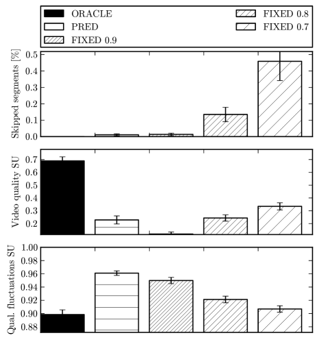
Figure 1: Evaluation results: fraction of skipped segments (reduced by "unplayable" segments), video quality subutility, and quality fluctuations subutility. Vertical lines display confidence intervals for a confidence level of 0.9.

In this section, we present the results of the evaluation of the proposed adaptation method based on simulations using throughput traces described in Section 3. Its performance is compared to the baseline approach using a fixed margin between past average throughput and the MMBR of the selected representation. It is further compared to the performance of an approach that has perfect knowledge of future throughput for a limited time horizon.

We use the following performance metrics: fraction of skipped segments, mean video quality subutility, and mean quality fluctuations subutility, computed over individual streaming sessions, lasting for the duration of individual traces. The videos for the evaluation are taken from the dataset provided by Lederer et al. [24]. The segment duration equals 2 seconds. For each video, we are using 10 representations, with MMBR’s ranging from 100 to 4200 kbps.

Some of the traces contain short periods when the throughput falls below the lowest available segment MMBR, so that a certain fraction of segments inevitably has to be skipped, independent of the deployed adaptation strategy. In order to compute this fraction, we simulate an adaptation algorithm that always selects the lowest representation, leading to a video quality subutility of 0 and a quality fluctuations subutility of 1. In the following, when we present the fraction of skipped segments for a simulation run, we always subtract the fraction of such "unplayable" segments.

The performance of the developed approach is compared to a baseline approach that uses a fixed margin between past average throughput and the MMBR of the selected representation. The margin is varied between 0.7 and 0.9. Effectively, this means that the baseline approach uses SMA:1:ar to predict throughput, assumes that the prediction is always an overestimate, and that the relative error is fixed.

We also compare to an oracle-based approach which has full knowledge about future throughput for a horizon of 10 seconds, and which selects for the next segment the highest representation that does not result in rebuffering within this time horizon.

We set the maximum playback delay to $\Delta^{p}_{\text{max}}=5$ seconds, which corresponds to a maximum transmission delay of $\Delta^{p}_{\text{max}}-\tau=3$ seconds, that is, 1.5 times the segment duration. Theoretically it is possible to further reduce the maximum transmission delay to equal segment duration, which, however, we consider infeasible since it would dramatically increase system’s sensitivity to throughput fluctuations.

We set $\alpha_{\text{cdf}}=60$. That is, the error for a prediction 2 seconds into the future is computed by estimating CDF parameters from past $2\alpha_{\text{cdf}}=120$ seconds. We set $\alpha_{\text{RB}}=-200$, which results in a steeply decreasing rebuffering subutility, since we define it our highest priority to avoid rebuffering, potentially sacrificing video quality and taking into account quality fluctuations.

Finally, we set $\alpha_{\text{Q}}=0.6$, giving quality subutility a slightly higher weight for the overall utility, than the quality fluctuations subutility.

The results of the evaluation are depicted in Figure 1. With the proposed algorithm, the mean fraction of skipped segments, without "unplayable" segments, is measured at approximately $10^{-4}$. This means that on average, a segment that could be played if perfect knowledge about future throughput would be available is skipped every half an hour. Recall that our highest priority is to keep the rebuffering rate as low as possible. The study in [7], e.g., suggests that live stream viewers can be extremely sensitive to rebuffering and might quit a streaming session after experiencing a single rebuffering event after a long time of uninterrupted viewing.

The mean quality subutility amounts to approximately one third of what is achieved given perfect knowledge about future throughput. The remaining two thirds constitute the inevitable tribute to the uncertainty of future throughput dynamics. Considering quality fluctuations, the proposed algorithm even achieves a higher subutility than the oracle approach.

We observe that in order to achieve a comparably small fraction of skipped segments using the fixed margin approach, a margin strictly greater than 0.9 is required (for exactly 0.9 the value is still slightly higher). At the same time, however, such a high margin results in significantly lower mean video quality and higher quality fluctuations. Further decreasing the margin downgrades the performance even more, leading to a fraction of skipped segments that is one order of magnitude higher.

Finally, we remark that in the present study we focused on network conditions with extremely high throughput fluctuations. Using the fixed margin approach on a link with moderate or low throughput fluctuations would further decrease resource utilization and thus further downgrade the performance. In the extreme case, if the throughput is constant, a fixed margin $x$ leads to a resource utilization of $1-x$. In contrast, since our algorithm dynamically estimates the relative prediction error, with constant throughput it is able to achieve a utilization close to 1. Thus, one of the strengths of the proposed method lies in its ability to perform equally well in very different network environments.

Chapter 7 Conclusion

In the presented study, we proposed an adaptation algorithm for HALS. It is based on the idea to compare potential future adaptation trajectories and to select the one maximizing QoE. QoE is evaluated based on a utility function depending on (i) the probability that a segment misses its playback deadline, (ii) the distortion of the video, and (iii) the number and amplitude of representation changes.

In order to compute the defined utility, in particular, the probability that a segment misses its playback deadline, we studied predictability of TCP throughput in wireless networks over timescales from 1 to 10 seconds. We evaluated different time series prediction methods using varying numbers of past throughput measurements. We demonstrated that the most naïve method, SMA, outperforms more sophisticated methods on all timescales, independent of the specific throughput dynamics. We further observed that prediction accuracy strongly varies across studied traces. Consequently, we studied approaches to model the prediction error and to estimate it for individual streaming sessions. We demonstrated that the overestimation error is extremely well represented by the Lomax distribution [22] on all considered timescales. The underestimation error is best represented by a truncated normal distribution except for the timescale of 1 second, where the truncated logistic distribution results in a slightly better Kolmogorov-Smirnov distance between the empirical and the theoretical CDF. In addition, we found out that although underestimations and overestimations are balanced over the total duration of individual traces, they exhibit a strong temporal correlation that we used to further improve prediction accuracy.

Using obtained insights, the proposed adaptation algorithm takes into account throughput predictions and an estimation of the relative prediction error, in order to maximize the defined QoE-based utility function. We evaluated the developed algorithm using collected throughput traces and showed that it outperforms the baseline approach which uses a fixed margin between past throughput and selected media bit rate.

Our ongoing and future work includes extending our collection of traces and including traces from mobile networks. It also includes studying the influence of ON/OFF patterns, generated by inter-request delays, on throughput prediction accuracy. Moreover, we are investigating how the prediction can be further improved by taking into account cross-layer information from TCP and MAC layers.

References

- [1] Radiotap. http://www.radiotap.org.
- [2] Definition of Terms Related to Quality of Service (ITU-T E.800). International Telecommunication Union Recommendation, 2008.
- [3] Vocabulary for Performance and Quality of Service, Amendment 2: New Definitions for Inclusion in Recommendation ITU-T P.10/G.100. International Telecommunication Union Recommendation, 2008.
- [4] MPEG-DASH (ISO/IEC 23009-1). Standard, 2012.
- [5] Cisco Visual Networking Index: Forecast and Methodology, 2013 - 2018. Cisco, Inc. Report, 2014.
- [6] U.S. Digital Future in Focus. comScore, Inc. Whitepaper, 2014.
- [7] Viewer Experience Report. Conviva Report, 2014.
- [8] Internet TV: Bringing Control to Chaos. Conviva Whitepaper, 2015.
- [9] YouTube Statistics. http://www.youtube.com/yt/press/statistics.html, 2015.
- [10] Cristina Aurrecoechea, Andrew T. Campbell, and Linda Hauw. A Survey of QoS Architectures. Multimedia Systems, 6(3):138–151, 1998.
- [11] Athula Balachandran, Vyas Sekar, Aditya Akella, Srinivasan Seshan, Ion Stoica, and Hui Zhang. A Quest for an Internet Video Quality-of-Experience Metric. In In Proc. of ACM Workshop on Hot Topics in Networks (HotNets), Redmond, WA, USA, 2012.
- [12] Athula Balachandran, Vyas Sekar, Aditya Akella, Srinivasan Seshan, Ion Stoica, and Hui Zhang. Developing a Predictive Model of Quality of Experience for Internet Video. In Proc. of ACM SIGCOMM, Hong Kong, 2013.
- [13] Tom Broxton, Yannet Interian, Jon Vaver, and Mirjam Wattenhofer. Catching a Viral Video. Journal of Intelligent Information Systems, 40(2):241–259, December 2013.
- [14] Jorge Carapinha, Roland Bless, Christoph Werle, Konstantin Miller, Virgil Dobrota, Andrei Bogdan Rus, Heidrun Grob-Lipski, and Horst Roessler. Quality of Service in the Future Internet. In In Proc. of ITU-T Kaleidoscope, Pune, India, 2010.
- [15] Jia Hao, Roger Zimmermann, and Haiyang Ma. GTube: Geo-Predictive Video Streaming over HTTP in Mobile Environments. In In Proc. of ACM Multimedia Systems Conference (MMSys), Singapore, 2014.
- [16] Myles Hollander, Douglas A. Wolfe, and Eric Chicken. Nonparametric Statistical Methods. Wiley, 2014.
- [17] T. Hossfeld, Sebastian Egger, Raimund Schatz, Markus Fiedler, Kathrin Masuch, and C. Lorentzen. Initial Delay vs. Interruptions: Between the Devil and the Deep Blue Sea. In In Proc. of Workshop on Quality of Multimedia Experience (QoMEX), Yarra Valley, Australia, 2012.
- [18] Rob J. Hyndman and Yeasmin Khandakar. Automatic Time Series Forecasting: The Forecast Package for R. Journal of Statistical Software, University of California, Los Angeles, Department of Statistics, 27(3):1–22, 2008.
- [19] Rob J. Hyndman, Maxwell L. King, Ivet Pitrun, and Baki Billah. Local Linear Forecasts Using Cubic Smoothing Splines. Australian & New Zealand Journal of Statistics, 47(1):87–99, 2005.
- [20] Dmitri Jarnikov and Tanır Özçelebi. Client Intelligence for Adaptive Streaming Solutions. Signal Processing: Image Communication, 26(7):378–389, August 2011.
- [21] Junchen Jiang, Vyas Sekar, and Hui Zhang. Improving Fairness, Efficiency, and Stability in HTTP-Based Adaptive Video Streaming with FESTIVE. In In Proc. of ACM Conference on emerging Networking EXperiments and Technologies (CoNEXT), Nice, France, 2012.
- [22] Norman Lloyd Johnson, Samuel Kotz, and Narayanaswamy Balakrishnan. Continuous Univariate Distributions. Wiley, 1994.
- [23] Dilip Kumar Krishnappa, Divyashri Bhat, and Michael Zink. DASHing YouTube: An Analysis of Using DASH in YouTube Video Service. In In Proc. of IEEE Conference on Local Computer Networks (LCN), Sydney, Australia, 2013.
- [24] Stefan Lederer, Christopher Müller, and Christian Timmerer. Dynamic Adaptive Streaming over HTTP Dataset. In In Proc. of ACM Multimedia Systems Conference (MMSys), Chapel Hill, NC, USA, 2012.
- [25] Blazej Lewcio, Benjamin Belmudez, Theresa Enghardt, and Sebastian Möller. On the Way to High-Quality Video Calls in Future Mobile Networks. In In Proc. of International Workshop on Quality of Multimedia Experience (QoMEX), Mechelen, Belgium, 2011.
- [26] Baochun Li, Zhi Wang, Jiangchuan Liu, and Wenwu Zhu. Two Decades of Internet Video Streaming: A Retrospective View. ACM Transactions on Multimedia Computing, Communications, and Applications, 9(1s):1–20, 2013.
- [27] Chenghao Liu, Imed Bouazizi, and Moncef Gabbouj. Rate Adaptation for Adaptive HTTP Streaming. In In Proc. of ACM Multimedia Systems Conference (MMSys), San Jose, CA, USA, 2011.
- [28] Xi Liu, Florin Dobrian, Henry Milner, Junchen Jiang, Vyas Sekar, Ion Stoica, and Hui Zhang. A Case for a Coordinated Internet Video Control Plane. In In Proc. of ACM SIGCOMM, Helsinki, Finland, 2012.
- [29] Yan Liu and Jack Y. B. Lee. On Adaptive Video Streaming with Predictable Streaming Performance. In In Proc. of IEEE Global Communications Conference (GLOBECOM), Austin, TX, USA, 2014.
- [30] Konstantin Miller, Emanuele Quacchio, Gianluca Gennari, and Adam Wolisz. Adaptation Algorithm for Adaptive Streaming over HTTP. In Proc. of the Packet Video Workshop, Munich, Germany, 2012.
- [31] Ricky K. P. Mok, Xiapu Luo, Edmond W. W. Chan, and Rocky K. C. Chang. QDASH: A QoE-Aware DASH System. In In Proc. of ACM Multimedia Systems Conference (MMSyS), Chapel Hill, NC, USA, 2012.
- [32] Tim O’Reilly. What Is Web 2.0: Design Patterns and Business Models for the Next Generation of Software. Communications & Strategies, 1:17–37, 2007.
- [33] Toon De Pessemier, Katrien De Moor, Wout Joseph, Lieven De Marez, and Luc Martens. Quantifying the Influence of Rebuffering Interruptions on the User’s Quality of Experience During Mobile Video Watching. IEEE Transactions on Broadcasting, 59(1):47–61, 2013.
- [34] Huynh-Thu Quan and Mohammed Ghanbari. Temporal Aspect of Perceived Quality in Mobile Video Broadcasting. IEEE Transactions on Broadcasting, 54(3):641–651, 2008.
- [35] Ulrich Reiter, Kjell Brunnström, Katrien De Moor, Mohamed-Chaker Larabi, Manuela Pereira, Antonio Pinheiro, Junyong You, and Andrej Zgank. Factors Influencing Quality of Experience. In Quality of Experience, pages 55–74. Springer International Publishing, 2014.
- [36] Haakon Riiser, Tore Endestad, Paul Vigmostad, Carsten Griwodz, and Pal Halvorsen. Video Streaming Using a Location-Based Bandwidth-Lookup Service for Bitrate Planning. ACM Transactions on Multimedia Computing, Communications, and Applications, 8(3):1–19, 2012.
- [37] Michael Seufert, Sebastian Egger, Martin Slanina, Thomas Zinner, Tobias Hossfeld, and Phuoc Tran-Gia. A Survey on Quality of Experience of HTTP Adaptive Streaming. IEEE Communications Surveys & Tutorials, to appear, 2014.
- [38] Kamal Deep Singh, Yassine Hadjadj-Aoul, and Gerardo Rubino. Quality of Experience Estimation for Adaptive HTTP/TCP Video Streaming Using H.264/AVC. In In Proc. of IEEE Consumer Communications and Networking Conference (CCNC), Las Vegas, NV, USA, 2012.
- [39] Iraj Sodagar. The MPEG-DASH Standard for Multimedia Streaming Over the Internet. IEEE Multimedia, 18(4):62–67, 2011.
- [40] Wei Song and Dian W. Tjondronegoro. Acceptability-Based QoE Models for Mobile Video. IEEE Transactions on Multimedia, 16(3):738–750, 2014.
- [41] Thomas Stockhammer. Dynamic Adaptive Streaming over HTTP – Standards and Design Principles. In In Proc. of ACM Multimedia Systems Conference (MMSys), San Jose, CA, USA, 2011.
- [42] Paul Sweeting. Video in 2014: Going Live and Over the Top. Gigaom Research Report, 2014.
- [43] Guibin Tian and Yong Liu. Towards Agile and Smooth Video Adaptation in Dynamic HTTP Streaming. In In Proc. of ACM Conference on emerging Networking EXperiments and Technologies (CoNEXT), Nice, France, 2012.
- [44] Bing Wang, Jim Kurose, Prashant Shenoy, and Don Towsley. Multimedia streaming via TCP: An analytic performance study. ACM Transactions on Multimedia Computing, Communications, and Applications, 4(2):1–22, May 2008.
- [45] Xiaoqi Yin, Vyas Sekar, and Bruno Sinopoli. Toward a Principled Framework to Design Dynamic Adaptive Streaming Algorithms over HTTP. In In Proc. of ACM Workshop on Hot Topics in Networks (HotNets), Los Angeles, CA, USA, 2014.
- [46] Liu Yitong, Shen Yun, Mao Yinian, Liu Jing, Lin Qi, and Yang Dacheng. A Study on Quality of Experience for Adaptive Streaming Service. In In Proc. of IEEE International Conference on Communications (ICC) Workshops, 2013.
- [47] Qian Zhang, Guijin Wang, Wenwu Zhu, and Ya-Qin Zhang. Robust Scalable Video Streaming over Internet with Network-Adaptive Congestion Control and Unequal Loss Protection. In In Proc. of Packet Video Workshop, Kyongju, Korea, 2001.