Beasts of the Southern Wild: Discovery of nine Ultra Faint satellites in the vicinity of the Magellanic Clouds.
Abstract
We have used the publicly released Dark Energy Survey data to hunt for new satellites of the Milky Way in the Southern hemisphere. Our search yielded a large number of promising candidates. In this paper, we announce the discovery of 9 new unambiguous ultra-faint objects, whose authenticity can be established with the DES data alone. Based on the morphological properties, three of the new satellites are dwarf galaxies, one of which is located at the very outskirts of the Milky Way, at a distance of 380 kpc. The remaining 6 objects have sizes and luminosities comparable to the Segue 1 satellite and can not be classified straightforwardly without follow-up spectroscopic observations. The satellites we have discovered cluster around the LMC and the SMC. We show that such spatial distribution is unlikely under the assumption of isotropy, and, therefore, conclude that at least some of the new satellites must have been associated with the Magellanic Clouds in the past.
Subject headings:
Galaxy: halo, galaxies: dwarf, globular clusters: general, galaxies: kinematics and dynamics1. Introduction
Currently, there are no strong theoretical predictions as to the luminosity function and the spatial distribution of the Galactic dwarf companions. In other words, today’s semi-analytic models are so flexible they can easily produce any number of Milky Way (MW) satellites: from a few tens up to several thousands (e.g. Koposov et al., 2009). Similarly, a large range of spatial arrangements is possible: from nearly isotropic to strongly planar (e.g. Bahl & Baumgardt, 2014). This is why to improve our understanding of the physics of the Universal structure formation on small-scales we look to observations. However, to date, only a third of the sky has been inspected. The Sloan Digital Sky Survey (SDSS) has demonstrated the power of deep wide-area imaging to fuel resolved stellar populations studies of the Galactic halo. The analysis of the SDSS data covering only 1/5 of celestial sphere has more than doubled the number of the known Galactic dwarf satellites (see e.g. Willman, 2010; Belokurov, 2013). Recently, both PanSTARRS and VST ATLAS have expanded the surveyed region significantly, but found little of the wealth they came to seek (Laevens et al., 2014; Belokurov et al., 2014).
The SDSS discoveries extended the dwarf galaxy regime to extremely low luminosities and sizes. As a result of adding these new faint surface-brightness objects (known as ultra-faint dwarfs, UFDs) to the panoply of Milky Way companions, it has been revealed that there appears to be a gap in the distribution of effective radii between globular clusters and dwarfs which extends across a large range of luminosities. In the absence of a working definition of a galaxy, an ad hoc combination of morphological, kinematic and chemical properties is required to be classified as one. Therefore, some objects that live dangerously close to the notional gap may risk misclassification. These faintest of the UFDs are only detectable with surveys like SDSS out to a small fraction of the MW virial radius. As a result, their total number in the Galaxy must be reconstructed under the assumption of the shape of their galactocentric radial distribution. Given that only a handful of such objects are known today, their radial profile is not observationally constrained. However, if it is assumed that the faintest of the UFDs are linked to the small-mass field dark matter (DM) sub-halos, their distribution can be gleaned from cosmological zoom simulations. This is an example of so-called sub-halo abundance matching which predicts that the bulk of the Galactic dwarf galaxy population is in objects with luminosities . The details of the semi-analytic calculations may vary but the result remains most astounding: there ought to be hundreds of galaxies with , if the faintest of the UFDs occupy field DM sub-halos (see e.g. Tollerud et al., 2008; Bullock et al., 2010).
It is, however, possible that the smallest of the UFDs may have been acquired via a different route. It has been suggested that some of these objects may have been accreted as part of a group (see e.g. Belokurov, 2013). In the case of the UFD Segue 2 for example, the group’s central object appears to have been destroyed and can now be detected only as tidal debris in the MW halo (Belokurov et al., 2009; Deason et al., 2014). In this scenario, the satellites of satellites survive (unlike their previous host) in the MW halo, but their spatial distribution should differ dramatically from that predicted for the accreted field sub-halos. Not only the radial density profile is modified, the satellites’ morphological properties might have been sculpted by the pre-processing (see e.g. Wetzel et al., 2015). Thus, the total numbers of the UFDs would be biased high if estimated through simple abundance matching calculation, while their spatial anisotropy would be greatly under-estimated.
On the sky, the remaining uncharted territory lies beneath declination and is currently being explored by the rapidly progressing Dark Energy Survey (DES). This is the realm of the Magellanic Clouds, long suspected to play a role in shaping the Galactic satellite population. For example, Lynden-Bell (1976) points out the curious alignment between several of the Milky Way dwarfs and the gaseous stream emanating from the Magellanic Clouds. Kroupa et al. (2005) developed this picture, adding more Milky Way satellites to the Great Magellanic family. The idea also receives support from the planar structures of satellites around M31 and other nearby galaxies (see e.g., Ibata et al., 2013; Tully et al., 2015). To explain the peculiar orbital arrangement of the Large Magellanic Cloud (LMC) and the fainter dwarfs within the CDM paradigm, D’Onghia & Lake (2008) consider a cosmological zoom simulation of accretion of an LMC-type object onto a Milky Way-size galaxy. In their simulation, approximately 1/3 of the satellites around the prototype MW at redshift come from the LMC group. They conjecture that the process of dwarf galaxy formation at the epochs around the re-ionisation is favoured in group environments, suggesting that at least in part, this can be explained by a significant difference in gas cooling times in the halo of a large galaxy like MW and a small group of the size of the LMC.
In this paper, we announce the discovery of a large number of new faint satellites detected via an automated stellar over-density search in the DES public release data. The paper is structured as follows. Section 2 outlines the steps required to produce object catalogues from the calibrated DES image frames. Section 3 presents the details of the satellite search routine. Section 4 gives an overview of the properties of the detected satellites, while Section 5 discusses their spatial distribution. The paper closes with Discussion and Conclusions in Section 6.
2. DES Data Processing
DES enjoys the use of the 2.2-degree field-of-view of the 570 megapixel DECam camera mounted on the 4m Blanco telescope at Cerro Tololo in Chile to obtain deep images of an extensive swath of the Southern sky around the Magellanic Clouds. DES is an international collaboration, whose primary focus is on the extra-galactic science. DES started taking data in August 2013 and will continue for five years. Currently, all its data products are proprietary, but the individual processed images are eventually released to the community through the NOAO infrastructure with a 1 year delay. In this paper, we present the results of the analysis of the entire DES imaging data released to date, i.e. 2100 square degrees obtained in the year of operations. Here, we concentrate on what clearly is a by-product of the DES survey: the stellar photometry and astrometry.
The NOAO Science Archive111http://www.portal-nvo.noao.edu/ hosts both raw and processed DES images. We have queried the database through the interface provided and selected all available InstCal calibrated images, the corresponding weight maps and the masks222The exact query used to select images from the NOAO Science archive: SELECT reference, dtpropid, surveyid, release_date, start_date, date_obs, dtpi, ra, dec, telescope, instrument, filter, exposure, obstype, obsmode, proctype, prodtype, seeing, depth, dtacqnam, reference AS archive_file, filesize, md5sum FROM voi.siap WHERE release_date ’2015-01-18’ AND (proctype = ’InstCal’) AND (prodtype IS NULL OR prodtype ’png’)) AND (dtpropid ILIKE ’%2012B-0001%’ OR surveyid ILIKE ’%2012B-0001%’) . The images were first staged for the download, and subsequently copied across for further processing. The total size of the released images, weight maps and masks in Rice compressed format was 4.6 TB. Once uncompressed, the size of the images and weight maps increases by a factor of 10. For the analysis reported below, only , and band images were analysed ( 30 TB of data).
DES images are taken with 90s exposure and the DECam pixel scale is 0.26′′/pixel. InstCal products, delivered by the DECam pipeline, are single-frame images (not stacks) that have been bias, dark and flat-field calibrated as well as cross-talk corrected. Additionally, defects and cosmic rays have been masked and the WCS astrometry provided333Detailed information available through the DECam Data Handbook at http://bit.ly/1D7ZGDc.
2.1. From Images to Catalogues
For the subsequent catalogue creation, we have relied heavily on the SExtractor/PSFEx routines (see Bertin & Arnouts, 1996; Bertin, 2011; Annunziatella et al., 2013, for more details). Typically, processing a single frame consisting of 60 CCD chips with SExtractor/PSFEx took 2.5 CPU-hours, leading to a total budget for the three DES filters of 15000 CPU-hours. The image processing has been carried out using the Darwin HPC computing facility444 http://www.hpc.cam.ac.uk as well as a local 8 node/96 core computer cluster. The main catalogue assembly steps are as follows:
-
•
Initial SExtractor pass. To provide the starting parameters for the PSFEx routine, the DES images are analysed by SExtractor. The flag settings are standard, albeit the
PHOT_APERTURESflag is adjusted to match the value of theG_SEEINGkeyword in the header (if it is available). Additionally, the downloaded weight maps are provided to SExtractor via theWEIGHT_MAPoption. -
•
PSFEx run. The output of SExtractor is used to calculate the PSFs for the subsequent photometry. PSFEx is run on each CCD chip separately with default PSFEx options, except the
PSF_SIZEkeyword which is set to (40,40) pixels. -
•
Final SExtractor pass. Using the PSF models computed in the previous step, SExtractor is run again to determine Model and PSF magnitudes. This step is the longest in the entire sequence.
-
•
Ingestion. For each filter, the resulting SExtractor catalogues are ingested into a PostgreSQL database as separate tables.
Q3Cspatial indices (Koposov & Bartunov, 2006) are created to speed up further steps. -
•
Duplicate removal. Due to significant image overlaps, sources appearing more than once have to be flagged in the catalogues. For each source we perform a search with 1 radius, and mark all objects coming from different frames and HDUs as secondary.
-
•
Photometric calibration. To convert instrumental magnitudes into calibrated ones for each frame (including multiple HDUs) a cross-match between the DES and the APASS DR7 survey data is performed. The zero-point is then measured as a median offset with respect to the APASS photometry on a per-field basis. The resulting photometric precision as estimated using overlaps of different frames is: 0.03 mag (Gaussian ) in the g-band, 0.025 mag in the r-band, and 0.033 mag in the i-band.
-
•
Band-merging. The lists of primary sources in the , and bands are combined into the final catalogue using the matching radius of 1 arcseconds. For the purpose of this paper, the catalogue was based on -band, i.e. -band detection was required in order for the object to be in the final catalogue.
-
•
The final
Q3Cindex is created on the band-merged catalogue to speed up spatial searches in the dataset.
2.2. Photometry and star-galaxy separation
| Name | SignifaaSignificance of detection in (t-value) | mMbbThe uncertainty in distance modulus is estimated to be 0.10.2 mag | Dist⊙bbThe uncertainty in distance modulus is estimated to be 0.10.2 mag | MV | r1/2ccHalf-light radius takes into account the ellipticity of the object via multiplier | r1/2ddThe error on distance was not propagated to the physical size | ellipticity | PA | BFeeBayes factor for the elliptical vs circular model | |||
|---|---|---|---|---|---|---|---|---|---|---|---|---|
| [deg] | [deg] | icance | [mag] | [kpc] | [mag] | [arcmin] | [arcmin] | [pc] | [deg] | |||
| Reticulum 2 | 48.5 | 17.4 | 30 | -2.70.1 | 711 | 1000 | ||||||
| Eridanus 2 | 31.5 | 22.9 | 380 | -6.60.1 | 816 | 1113 | ||||||
| Horologium 1 | 28.4 | 19.5 | 79 | -3.40.1 | 0.35 | |||||||
| Pictoris 1 | 17.3 | 20.3 | 114 | -3.10.3 | 7823 | 1.41 | ||||||
| Phoenix 2 | 13.9 | 19.6 | 83 | -2.80.2 | 16454 | 1.81 | ||||||
| Indus 1 | 13.7 | 20.0 | 100 | -3.50.2 | 0.46 | |||||||
| Grus 1ffAs this object is located very close to the CCD chip gap, its morphological properties should be treated with caution | 10.1 | 20.4 | 120 | -3.40.3 | 460 | 1.01 | ||||||
| Eridanus 3 | 10.1 | 19.7 | 87 | -2.00.3 | 8336 | 0.81 | ||||||
| Tucana 2 | 8.3 | 18.8 | 57 | -3.80.1 | 10718 | 2.14 |
Note. — Morphological parameters of the satellites are maximum a posteriori estimates with 68% (1) credible intervals, or limits
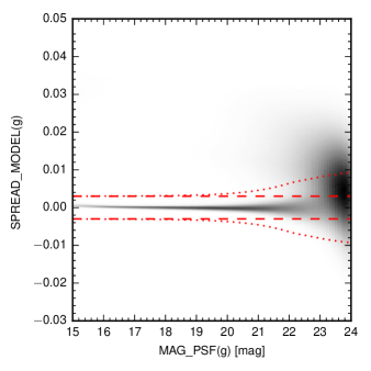
PSF magnitudes of star-like objects are given by the MAG_PSF
output of SExtractor. As an indicator of star-galaxy separation we
use the SPREAD_MODEL parameter provided by SExtractor. This
is a metric similar to psfmag-modelmag used by SDSS (see
Fig. 1). A sensible selection threshold for bright
stars would be (Desai et al., 2012; Annunziatella et al., 2013), however
for faint magnitudes this cut causes significant incompleteness in
stars. Therefore, instead we choose to
require:555http://1.usa.gov/1zHCdrq
| (1) |
This particular cut ensures that the stellar completeness remains
reasonably high at faint magnitudes, while the contamination is kept
low at the same time. The behaviour of
as a function of magnitude shown in Figure 1 explains
why a fixed SPREADERR_MODEL threshold is suboptimal. To assess
the levels of completeness and contamination induced by our stellar
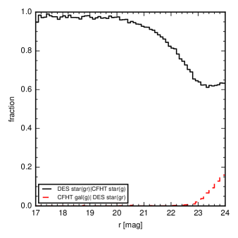
selection, we use a portion of the DES-covered area of sky overlapping
with the CFHTLS Wide survey (Hudelot et al., 2012). This is a dataset of
comparable depth, for which morphological object classifications are
provided. Figure 2 gives the resulting
performance of the stellar selection procedure in which Equation
1 is applied to both and -band catalogues. In
particular, the Figure gives completeness (black solid histogram)
calculated as the fraction of objects classified as stars by CFHTLS
(their CLASS_STAR0.5) which are also classified as stars by
our cuts applied to the DES data. Similarly, contamination can be
gleaned from the fraction of objects classified as galaxies by the
CFHTLS but as stars by our DES cuts (red dashed line). It is
reassuring to observe low levels of contamination all the way to the
very magnitude limit of the DES survey. At the same time, completeness
is high across a wide range of magnitudes and only drops to
60% for objects fainter than . It is also worth noting that
the star-galaxy separation criteria employed in this work may not be
ideally suited for other studies, as they may have different
requirements in terms of the balance between the completeness and the
contamination.
In the stellar catalogues built using the procedure described above, the magnitudes are equivalent to the SDSS . Consequently, the extinction coefficients used are those suitable for the SDSS photometric system, while the dust reddening maps employed are from Schlegel et al. (1998). Note that the depth of the resulting catalogues varies somewhat across the DES footprint, but could be approximately estimated from the source number counts in , , filters. These number counts peak at magnitudes 23.7, 23.6, 22.9 in , , correspondingly, indicating that the catalogues start to be significantly affected by incompleteness at somewhat brigher magnitudes g23.5, r23.4, i22.7.
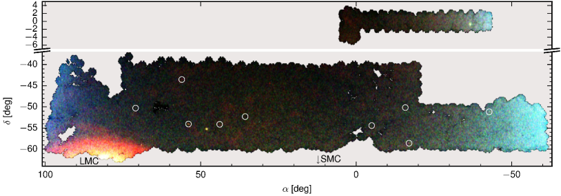
To illustrate the quality of the resulting catalogue, Figure 3 displays the density of the Main Sequence Turn-Off (MSTO; 0.2gr0.6) stars on the sky. The density of stars with 19r21 (corresponding to distances of 1025 kpc) is shown in the green channel, more distant stars with 21r22.75 (corresponding to distances of 2556 kpc) are used for the red channel, and the nearby stars with 17r19 (distances of 410 kpc) in the blue channel. This map is an analog of the ”Field of Streams” picture by Belokurov et al. (2006). The density distribution is very uniform thus confirming the high precision and the stability of the photometry as well as the robustness of the star-galaxy separation across the survey area. The map also reveals some of the most obvious overdensities discovered in this work, at least two of which are visible as bright pixels in the Figure.
3. Search for stellar over-densities
To uncover the locations of possible satellites lurking in the DES data, we follow the approach described in Koposov et al. (2008); Walsh et al. (2009). In short, the satellite detection relies on applying a matched filter to the on-sky distributions of stars selected to correspond to a single stellar population at a chosen distance. The matched filter is simply a difference of 2D Gaussians, the broader one estimating the local background density, while the narrow one yielding the amplitude of the density peak at the location of the satellite.
We start by taking a catalogue of sources classified as stars. A sub-set of these is then carved out with either a set of colour-magnitude cuts or with an isochrone mask offset to a trial distance modulus. Then a 2D on-sky density map of the selected stars is constructed, keeping the spatial pixel sufficiently small, e.g. 1′ on a side. At the next step, the density map is convolved with a set of matched filters (described above) with different inner and outer kernels. Finally, these convolved maps are converted into Gaussian significance maps and the most significant over-densities are extracted.
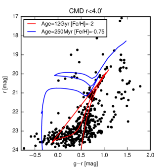
In the analysis presented here, we have used the mask based on the PARSEC isochrone (Bressan et al., 2012) with an age of 12 Gyr and metallicity of 666http://stev.oapd.inaf.it/cmd, spread out by the characteristic DES photometric error as a function of colour and magnitude. The trial distance moduli explored in the search range from mM=15 to mM=24. The inner kernel size is allowed to vary from 1 to 10. After extracting the most significant over-densities all detections are cross-matched with the list of positions of known dwarf galaxies from McConnachie (2012), nearby LEDA galaxies (Paturel et al., 2003) with radial velocities less than 2000 km/s, globular clusters in the catalogue of Harris (1996) as well as the globular clusters listed in Simbad.
The list of over-densities produced is then cleaned for duplicates, e.g. over-densities detected with more than one distance modulus and/or kernel size. We have also removed detections near the very edge of the survey’s footprint. The remaining candidates are ranked by their significance and eye-balled. Among the 9 objects presented in this paper, 5 are at the very top of the ranked list with significances well above 10, while a further 4 are somewhat lower in the list (but with significances of order of 10). We firmly believe that all objects presented below are genuine new satellites of the Milky Way. Apart from the over-density significance, our inference is based on a combination of additional factors, including their morphological and stellar population properties. We describe this overwhelming observational evidence in detail in the next Section. The list of objects and their properties is given in Table 1 and discussed in detail in the next Section.
4. Properties of the detected objects
While our search for stellar over-densities returned a large number of promising candidates, in this Paper we concentrate on a particular gold-plated sample of objects whose nature can be unambiguously established with the DES data alone. Let us briefly review the sanity checks carried out to corroborate the classification. First, each of the nine objects possesses a significant stellar overdensity, in fact, the significance is in excess of 10 in eight out of nine cases. Second, no obvious background galaxy overdensity is visible, thus reducing dramatically the possibility that the objects are spurious density peaks caused by mis-classified faint galaxies. Third, the dust maps in the vicinity of each of the satellite do not show any strong features that can be linked to the stellar overdensity. Most importantly, distributions of stars in the colour-magnitude plane reveal sequences corresponding to coeval populations at the same distance. In all cases, not just one particular stellar population is visible but several, for example, MSTO+RGB+BHB.
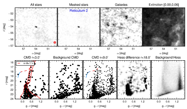
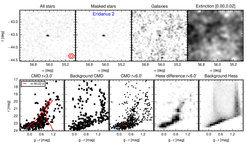
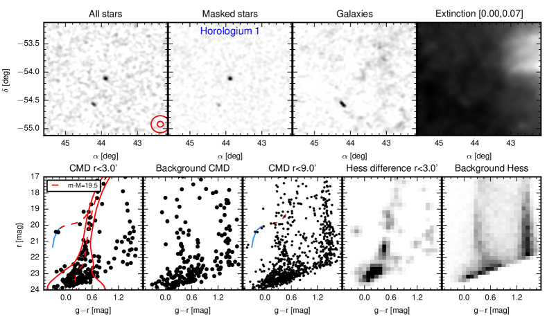
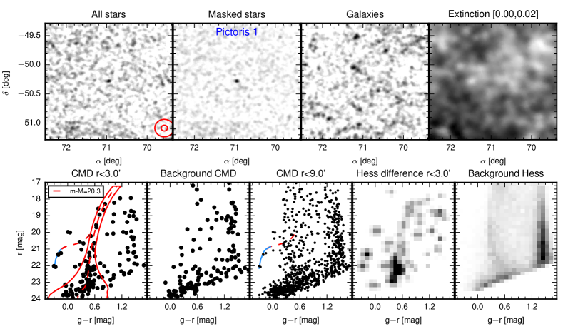
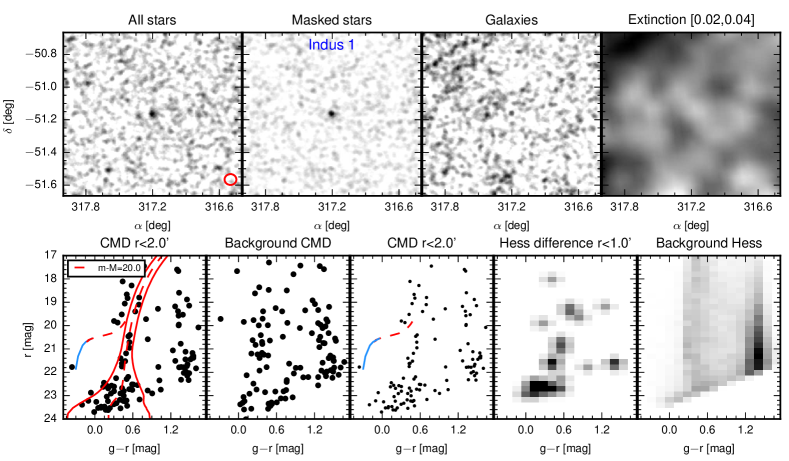
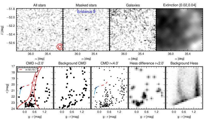
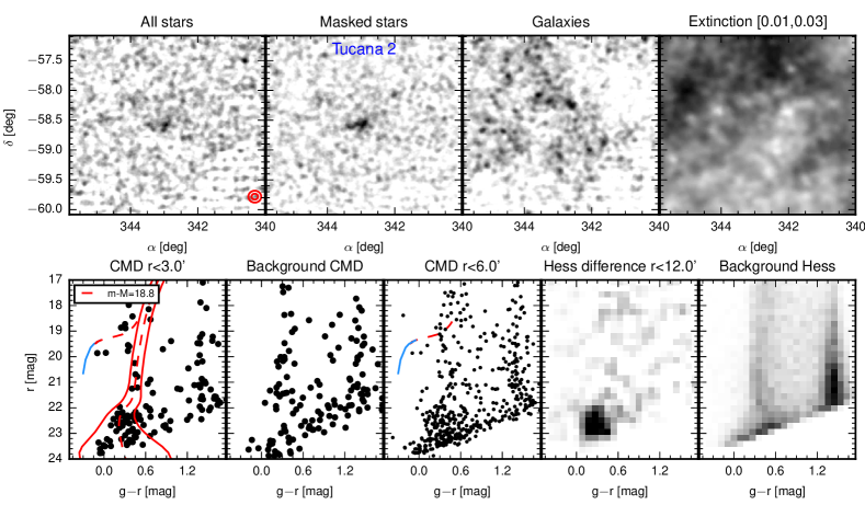
Figures 4-12 give the visual summary of the properties of each of the detected satellites and serve to substantiate our classification. Each of these diagnostic plots comprises of 9 panels: 4 in the top row are concerned with the on-sky distribution of the object’s stars, while the 5 in the bottom row give details of its stellar populations. In particular, the density of all objects classified as stars is shown in the top left panel. The second panel in the row gives the density of all stars selected with the best-fit isochrone mask (shown in the left bottom panel). For comparison, the density of objects classified as galaxies is presented in the third panel, and the galactic extinction map from Schlegel et al. (1998) in the fourth.
The first panel in the bottom row displays the colour-magnitude distribution of stars selected to lie in the small aperture (whose size is indicated by the small red circle in the bottom right corner of the top left panel) centered on the object. Red solid lines are the boundaries of the isochrone mask used to select the probable satellite member stars, while the isochrone itself is shown as a red dashed line. The horizontal branch (HB) in the model isochrone does not extend to sufficiently blue colours, therefore we complement the theoretical HB with a fiducial HB (blue solid line) built using data for the metal-poor old globular cluster M92 from Bernard et al. (2014). The object’s CMD can be contrasted to the foreground/background CMD shown in the second bottom panel. This is built with random nearby stars located within large annulus (typical inner radius 0.2 and outer radius of 1) and sampling the same number of stars as that in the left panel. The aperture chosen to create the CMD in the left panel is sufficiently small in order to minimize the contamination by non-member stars. This, however, implies that some of the rarer stellar populations (such as BHBs for example) are not fully sampled. A more complete view (albeit with a higher contamination) of the satellite’s stellar populations can be seen in the third bottom panel for which a larger aperture is used (large red circle in the top left panel). In most cases, this particular view of the CMD strengthens the detection of the BHB population. The last two panels in the bottom row are Hess diagrams, i.e. density distributions in the colour-magnitude space. In particular, the fourth panel is the Hess difference between the stars inside a small aperture centered on the satellite (the aperture size is shown in the panel’s title) and a large area well outside the satellite’s extent. Finally, for comparison, the Hess diagram of the background/foreground population is shown the fifth panel of the bottom row.
All objects we report in Table 1 have passed the sanity checks described above with flying colours. Moreover, some of the new satellites are actually visible in the DES image cutouts as described in the sub-section 4.2.
The naming convention we have adopted uses the constellation of the object together with the corresponding arabic numeral. This differs from the customary bimodal naming convention for globular clusters and dwarf galaxies, that leads to the name dependance on the knowledge of whether the object is a cluster or a galaxy.
4.1. Satellite modelling
Having identified the objects of interest, we proceed to measuring their distances, luminosities and structural parameters. First, the distances are determined using the available BHB stars if present. We have used both the theoretical HB isochrone corresponding to the old metal-poor population mask used for the selection of the likely satellite members and the M92 HB fiducial from Bernard et al. (2014) converted into the SDSS photometric system using the equations from Tonry et al. (2012). The distance moduli implied by these HBs are consistent within 0.1 mag. To verify the distance accuracy we also fitted the Hess diagram of each object with a stellar population model (see e.g. Koposov et al., 2010, for more details). For all objects (excluding Tucana 2) this gave us similar distance modulus differing by less than 0.1 - 0.2 mag. For Tucana 2 we use the distance implied by the Hess diagram fit.
To measure the morphological properties of all the detected objects, we have modelled the on-sky 2D distribution of the likely member stars (see e.g. Martin et al., 2008, for similar approach). For each object, only stars located within the CMD mask are used for the morphological analysis. The model used to describe the density distribution of stars is a mixture of the background/foreground stellar density (assumed to be constant across a few degrees around the object) and a rotated elongated exponential model for the satellite’s stars. Therefore, the probability of observing a star at a particular position on the sky with coordinates and is:
and
Here is the area of the analysed part of the data and is a shorthand notation for all model parameters, of which there are 6 in total. These are: - the fraction of objects belonging to the object, – the major axis (the exponential scale length), – ellipticity of the object, positional angle of the major axis, and finally, – the position of the center of the object.
The above model is fit to the data assuming uninformative priors on , flat priors on and PA, (i.e. e Uniform(0, 0.8), PA Uniform(0, 180)) and the Jeffreys priors on and , namely Beta(0.5, 0.5) and (see e.g. Mackay, 2002; Gelman et al., 2014). The resulting posterior is sampled using the Affine invariant Ensemble sampler (Goodman & Weare, 2010; Foreman-Mackey et al., 2013). The values of parameters and the associated uncertainties are given in Table 1. To check whether the ellipticity of an object is significant, the Bayes Factor is calculated using the Savage-Dickey ratio (Verdinelli & Wassermann, 1995; Trotta, 2007). As the Table 1 reports (final column), only Reticulum 2 and Eridanus 2 show strong, statistically significant elongation. Other objects are consistent with being circular.
Having modelled the morphology of each satellite, the posterior distributions of their structural paramereters are used to estimate the total number of stars belonging to the satellite. The satellite luminosities are calculated only with stars with r23 falling within the isochrone mask (we have used a brighter magnitude limit to avoid incompleteness due to the star/galaxy misclassification). Then, the number of stars inside the isochrone mask is converted into the stellar mass and the corresponding total luminosity assuming an old metal-poor isochrone and the KTG/Chabrier IMF (Kroupa et al., 1993; Chabrier, 2003).
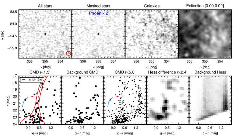
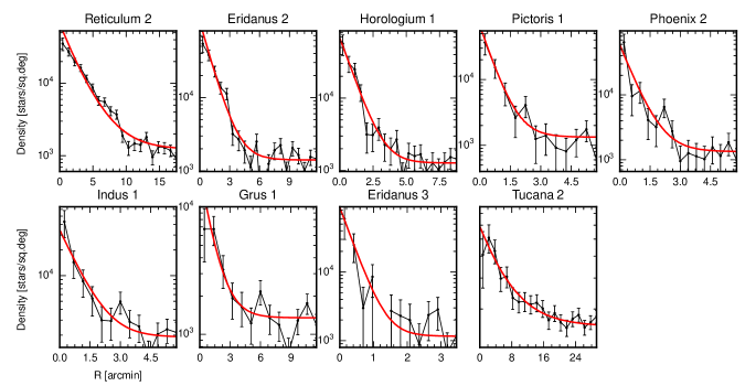
Figure 13 is a gallery of 1D azimuthally averaged stellar density profiles for each of the satellites. Red lines are the best fit exponential models. Before we discuss the size-luminosity distribution of our sample in sub-section 4.3, let us have a closer look at the individual properties of each of the satellites.
4.2. Notes on individual objects
-
•
Reticulum 2 (see Figure 4) – With the significance in excess of 40, this is the most obvious previously unknown object in the DES field of view. The CMD shows clear MS and MSTO together with beginnings of a RGB. Reticulum 2 is clearly very elongated: the measured axis ratio is around 0.6. It is one of the two objects in the sample presented here, for which the flattening of the stellar density is statistically significant. Its luminosity is and the half-light radius of 30 pc, which brings it just outside the cloud of classical globular clusters into either extented globular clusters or dwarf galaxies. It is impossible to classify this satellite securely with the data in hand, therefore we shall designate this and similar objects as ”ultra-faint satellites”. Clearly, kinematic and chemical analysis is required before the nature of this object can be established. It is reasonable to associate the low axis ratio measured for this object with the effects of the Galactic tides. However, at the moment, we do not have any firm evidence of extra-tidal material outside the satellite. The distance estimate for Reticulum 2 is 30 kpc as judged by a couple of BHB stars as well as the prominent MS and RGB. Note that eight other satellites are all substantially further away.
-
•
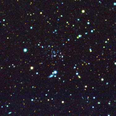
Eridanus 2 (see Figure 5). This is the second most significant and the most distant object in our list. With its location on the periphery of the Galaxy at 380 kpc, luminosity of and the size of 170 pc, this appears to be a twin of the Leo T dwarf galaxy (Irwin et al., 2007). Similarly to Leo T, Eridanus 2 is clearly visible in the DES color images (Figure 15) as a group of faint blue stars embedded in a blue low surface-brightness cloud. In contrast to Leo T though, Eridanus 2 shows significant elongation with a measured ellipticity of 0.4. Its color-magnitude diagram boasts a strong RGB and a very prominent red clump. Additionally, there appears to be a group of bright blue stars which could possibly be interpreted as young blue-loop stars (see Figure 16), similar to those found in Leo T (Weisz et al., 2012). The HB stars of Eridanus 2 are just at the magnitude limit achievable with the single-frame DES photometry. The possible presence of young stars and large distance to the Eridanus 2 galaxy suggest that the satellite is a viable candidate for follow-up HI observations. The color images of the galaxy (see both panels of Figure 15 also show an curious fuzzy object which can be interpreted as a very faint globular cluster. The object is almost at the center of the galaxy ()=() and is very diffuse with a size consistent with a few parsecs assuming it is at distance of Eridanus 2777There is another compact but high surface brightness round object looking consistent with a globular cluster ()= (56.0475,-53.5213) but it is probably a background galaxy as even its outskirts do not resolve into stars. If any of the faint diffuse objects superposed with Eridanus 2 are indeed globular clusters, this would make this satellite the faintest galaxy to possess stellar sub-systems!

Figure 10.— Grus 1. See Figure 4 for detailed description of the panels. Grus 1 is situated at a distance similar to that of Horologium 1, Pictoris 1, Phoenix 2 and Indus 1. The central stellar overdensity is not as prominent as in the previously discussed objects. This is partly explained by the fact that Grus 1 falls right into the CCD chip gap. Nonetheless, the CMD shows off such familiar features as an RGB and a well-populated HB. -
•
Horologium 1 (see Figure 6). This is the third most obvious object within the DES field-of-view with a significance of 30. Horologium 1 is one of 7 satellites all lying at approximately the same distance of 100 kpc. Both its Hess diagram and the CMD clearly show a prominent red giant branch as well as the group of the BHB stars. With a luminosity of and a size of 30 pc it sits within the uncertain territory where extended star cluster and faint dwarf galaxies start to overlap. We class it as an ”ultra-faint satellite”.
-
•
Pictoris 1 (see Figure 7). Another high significance ultra-faint satellite located at 115 kpc and projected near the LMC on the sky. The CMD shows a clear RGB and a few stars on the HB. Its size is 30 pc and its luminosity is .
-
•
Phoenix 2 (see Figure 8). An ultra-faint satellite at 80 kpc with the half-light radius of 26 pc and luminosity of . Apart from a clear MSTO and RGB, one or two BHB stars, there is potentially a large number of BS stars extending to gr0, r22.
-
•
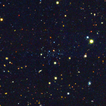
Indus 1 (see Figure 9). Similar to the bulk of our sample, this ultra-faint satellite is at 100 kpc with a half-light radius of 36 pc and the luminosity of . Interestingly, Indus 1 is conspicuous in the DES false-color image (see Figure 14).
At the time of the submission of this manuscript, the discovery of the same satellite was announced in Kim et al. (2015) where the object’s size and luminosity are quoted to be significantly lower than the values we obtain. Using imaging data much deeper than available to us, Kim et al. (2015) report the detection of a pronounced mass segregation, which (if true) would argue strongly in favour of the globular cluster nature of the object. Moreover, the disagreement in the inferred total luminosity can be explained by the difference in depth between the two datasets in the presence of a depletion at the low-mass end of the mass function. With regards to the extent of the object, we note that it is possible that our size determination has been biased high by blending in the central parts of the object. However, the small size reported by Kim et al. (2015) could, at least in part, be the consequence of the choice not to fit the stellar density at lager radius, as it is classified as “extra-tidal” by the authors.
-
•
Grus 1 (see Figure 10). The satellite is at 120 kpc, has a luminosity of and a size of 60 pc. Given its luminosity and size, the satellite should perhaps be classified as a dwarf galaxy. However, care should be taken when interpreting the measured structural parameters, as the object sits right at the CCD chip gap.
- •
-
•
Tucana 2 (see Figure 12). This satellite can perhaps be classified as an ultra-faint dwarf galaxy with less ambiguity than many others in the sample, due to its more substantial luminosity of and the large size of 160 pc. The extent of the object is immediately obvious from the map of selected stars (second panel in the top row). The CMD demonstrates a strong MSTO, a sub-giant branch. A few blue objects with colors consistent with the BHB stars are probably foreground contaminants as their magnitude contradicts the distance modulus implied by the subgiant branch. The estimated distance is 60 kpc
4.3. Size-luminosity relation
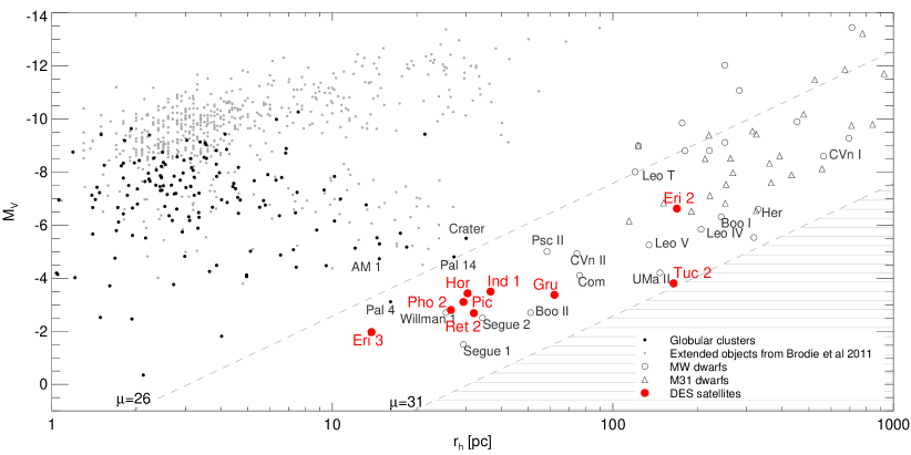
Figure 17 shows the locations of the discovered satellites on the plane of half-light radius ( and intrinsic luminosity (). Together with the objects in our sample (red filled circles), several other stellar systems are displayed. These include globulars clusters (GCs, black dots), MW dwarf galaxies (black unfilled circles), M31 dwarf galaxies (black empty triangles), as well as extended objects with half-light radius less than 100 pc from the catalogue of Brodie et al. (2011). Let us start by pointing out that all groups of objects in this compilation are affected by selection effects. Most importantly, the detectablility of all objects is dependent on their surface brightness. For objects detectable as resolved stellar systems in surveys similar to the SDSS, the parameter space below the surface-brightness limit of mag deg-2 (Koposov et al., 2008) is unexplored (see dashed lines of constant surface-brightness in the Figure). Additionally, there are constraints set by blending for star clusters, which deteriorate with increasing distance.
Notwithstanding various selection effects, star clusters and dwarf galaxies seem to occupy distinct regions of the size-luminosity plane. Brighter than , star clusters seem to rarely exceed half-light radius pc, while no dwarf galaxy is smaller than 100 pc. In other words, there seems to be a size gap between star clusters and dwarf galaxies. At fainter magnitudes, the picture is a lot more muddled. Not only are there objects firmly classified as dwarf galaxies with size under 100 pc (for example Pisces II and Canes Venatici II), but also several ultra-faint satellites, namely Segue 1, Segue 2 and Bootes 2 have sizes and luminosities comparable to faint extended globular clusters such as Palomar 4 and Palomar 14. What sets Segue 1,2 and Bootes 2 apart from similar looking star clusters are their chemical abundances. All three objects appear to have large metallicity spreads (e.g. Frebel et al., 2014; Kirby et al., 2013; Koch & Rich, 2014), previously unnoticed in star clusters.
Guided by the approximate shapes of the distribution of star clusters and dwarf galaxies in size-luminosity plane, we can conclude the following. Using the measured morphological parameters only, out of the 9 satellites, only three, namely Eridanus 2, Tucana 2 and Grus 1 can be classified as dwarf galaxies unambiguously, without having to resort to follow-up spectroscopy. We classify the remaining six, i.e. Eridanus 3, Phoenix 2, Horologium 1, Pictoris 1, Reticulum 2 and Indus 1 simply as ultra-faint satellites with the hope that their true nature is revealed through detailed abundance studies in the near future.
It is interesting that in the size luminosity plane the ambigiously classified objects in our sample seem to join the sequence of objects observed in other galaxies labelled as faint-fuzzies (FF) or Extended Clusters (EC) (see Larsen et al., 2001; Brodie et al., 2011; Forbes et al., 2013). These objects have sizes of tens of parsecs and luminosities of . While our objects are significantly fainter, one should take into account that most HST surveys of other galaxies are incomplete for objects with . The possible connection between FF/EC objects and the ultra-faint satellites is particularly intriguing given the likely association between some of our objects and the Magellanic Clouds (see Section 5).
Strikingly, while most of the new satellites announced here are rather faint, none of them lies particularly close to (with the exception of Tucana 2), or indeed below, the nominal surface brightness limit of . This means that these satellites are not very different from those discovered by Sloan (only somewhat more distant at fixed luminosity), and, therefore, significant fraction, but not all of them (as the objects lie very close to the luminosity vs distance limits of Koposov et al. (2008) and Walsh et al. (2009)) would have very likely been identified by the SDSS and the VST ATLAS had they fallen within the footprints of these surveys. The relatively high surface brightness values of the DES satellites must imply that we have not tapped into a large supply of nearly invisible dwarfs predicted by some of the semi-analytic models. Instead, the discovery of a large number of satellites from a small area as compared to the previously observed sky suggests a peculiar spatial distribution of these objects. This is the focus of the next Section.
5. Spatial distribution
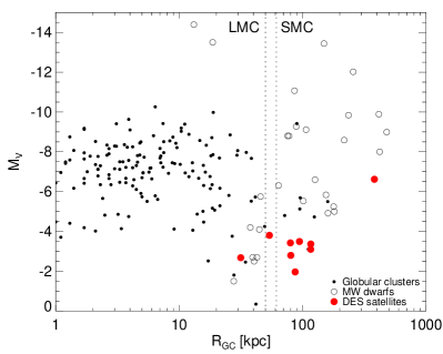
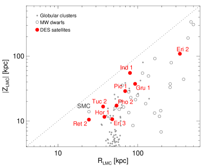
Let us start by inspecting the overall distance distribution of the DES satellites. Figure 18 gives the object’s luminosity as a function of Galacto-centric radius . It is immediately obvious that i) our satellites are some of the faintest of the distant MW satellites known, and ii) a large faction of them cluster around the distance kpc. In other words, the satellites as a group lie not far from the LMC ( kpc) and just behind the orbit of the Small Magellanic Cloud (SMC, kpc).
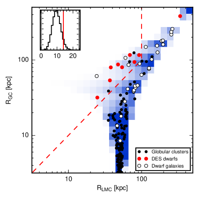
A more direct test of a possible association with the Magellanic Clouds is shown in Figure 19. Here we plot the distance to the LMC against the distance to the Galactic centre for the DES satellites as well the known MW dwarf galaxies (McConnachie, 2012) and globular clusters (Francis & Anderson, 2014). In this space, the objects that lie above the one-to-one diagonal line of the plot are closer to the LMC than to the Galactic centre. Note that all our objects lie above this demarcation line. While surprising at first, this is in fact expected due to the particular sky coverage of the DES survey (see Figure 3). However, even if the bunching around the Magellanic Clouds is set by the footprint, the total number of the satellites uncovered in such small area is alarming, especially when compared to the Southern portions of the SDSS, or VST ATLAS.
To test whether there is a statistically significant overdensity of satellites in the vicinity of the LMC we carry out the following calculation. The 3D position vector of each MW satellite, including the newly discovered ones, but excluding the LMC itself, is rotated randomly 50000 times with respect to the Galactic center (GC) while keeping fixed its Galacto-centric radius. After each rotation, the distance to the LMC is computed and stored. The blue/white background density in Figure 19 shows the average expected density of objects in the (, ) space from the random 3D position reshuffles described above. Under the assumption of an isotropic distribution of satellites in the Galaxy, our procedure would yield a reasonable estimate of the expected number of satellites in each portion of the (, ) plane. Darker shades of blue show areas where more objects are expected, while pale blue and white pixels correspond to less populated corners of the parameter space.
According to the simulation described above, the entire group of the satellites announced in this paper (excluding the distant Eridanus 2) is located in the under-populated area of the (, ) space, as indicated by the pale blue background density. This can be interpreted as a detection of an over-density of satellites around the LMC. To quantify the significance of this detection we perform the following frequentist hypothesis test. We carve the LMC-dominated area in the () space: and kpc. Then the total number of satellites in the LMC-dominated area (excluding LMC itself) is computed. The actual observed number () is compared to the number of objects in the marked region as given by the random reshuffles of the 3D position vectors. The distribution of the possible number of satellites in the marked area is shown in the inset of the Figure, and the observed number is given by the red vertical line. The distribution obtained assuming isotropy is narrow and peaks around , indicating the presence of a satellite overdensity in the DES data. However, the formal significance level of this result is not very high at 94%888The boundary in the vs space used for the test is chosen to be as simple as possible to avoid artificially inflating the p-value. while the estimated excess is also quite modest, i.e. of order of 4 objects.
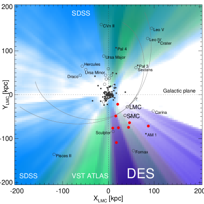
Having established a possible connection between the Magellanic Clouds and the DES satellites, we study the distribution of the new objects in the plane of the LMC’s orbit. Figure 20 shows the MW satellites (GCs, dwarfs and DES satellites) projected onto the plane defined by the vector of the LMC’s velocity as given in Kallivayalil et al. (2013)999 The transformation from the Galactocentric coordinates (X,Y,Z) (X is positive towards the Galactic anticenter) to shown in Figures 20 and 21 is defined by ; ; . . We also show the forward- and backward-integrated orbits of the LMC in two MW potentials with different DM halo concentrations ( and ). Coloured regions correspond to the fraction of the Galactic volume covered by the SDSS, VST ATLAS and DES surveys as projected onto the LMC’s orbital plane. The three slightly over-lapping surveys have together covered a large portion of the sky. However, some lacunae still remain, most notably directly in front of the LMC-SMC pair as judged by the vector of the LMC motion (black arrow). As expected, the DES satellites bunch tightly outside the SMC’s orbit. However, while the objects have similar in-plane coordinates, not all of our satellites actually lie close to the orbital plane of the LMC. The distance from the LMC’s orbital plane is shown in Figure 21. Only, Reticulum 2, Horologium 1 and Eridanus 3 have small heights above the plane kpc. The distribution of the other 6 objects do not show any strong alignment with the LMC’s orbit.
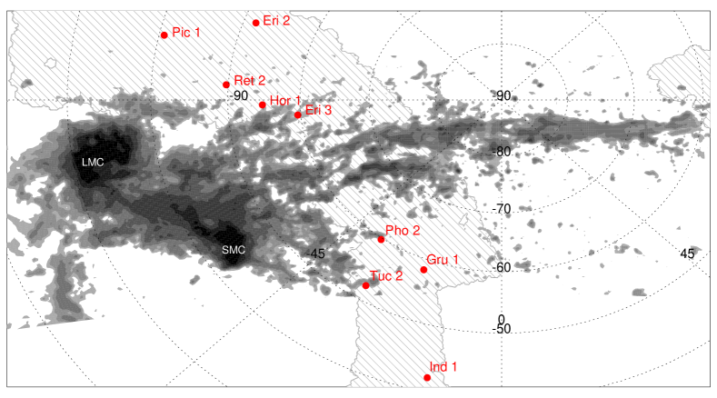
The accretion of the Magellanic system has left behind a trail of neutral hydrogen. Figure 22 compares the positions of the DES satellites to the distribution of HI in the Magellanic Stream as traced by Putman et al. (2003). Curiously, the DES satellites seem to avoid the high column density portions of the stream. The spatially distinct behavior of the gas and the stars is similar to that seen around M31 (Lewis et al., 2013). There is however possible overlap between Horologium 1, Eridanus 3, Phoenix 2 and Tucana 2 with the high velocity clouds associated with the Stream. Additionally, the particular projection used in the Figure emphasizes the fact that there appears to be two groups: one containing Pictoris 1, Eridanus 2, Reticulum 2, Horologium 1 and Eridanus 3, all lying on the LMC side of the Stream. Meanwhile, Phoenix 2, Tucana 2, Grus 1 and Indus 1 can be found on the SMC side. Interestingly, the three objects that have the highest probability of being aligned with the orbital plane of the LMC (see Figure 21), i.e. Reticulum 2, Horologium 1 and Eridanus 3 are the satellites closest to the Magellanic Stream.
6. Discussion and Conclusions
In this paper, we have presented the discovery of 9 new ultra-faint Milky Way satellites using the data from the Dark Energy Survey. Based on the morphological properties, 3 of the satellites are definite dwarf galaxies, while the exact type of the other 6 is more ambiguous. The nearest object in the sample shows a significant elongation indicative of the influence of the Galactic tides. The most distant object discovered appears to be a dwarf galaxy located at the very edge of the Milky Way halo, around 380 kpc. This remote dwarf shows signs of recent star formation and possibly even hosts a faint globular cluster! The discovery of a large number of MW satellites in a small area around the LMC and the SMC is suggesting that at least a fraction of the new objects might have once been a part of the Magellanic group.
The idea that some of the satellite galaxies of the Milky Way may be associated with the Magellanic Clouds is quite old. Let us re-visit the earlier work in the light of the discoveries in this paper.
Lynden-Bell (1976) first suggested the idea of a Greater Magellanic Galaxy. His paper predates modern ideas on galaxy formation, and so his picture is rather different from today’s concensus. He envisaged dwarf galaxies condensing from gas torn out of the Greater Magellanic Galaxy via a tidal encounter with the Milky Way Galaxy. He noted that Draco and Ursa Minor lie in the Magellanic Plane, almost opposite the Magellanic Clouds in the Galactocentric sky, and were candidates for debris from the break-up of the Greater Magellanic Galaxy. This speculation received some confirmation when Lynden-Bell (1982) showed that the elongation of Draco and Ursa Minor is along the Magellanic Stream. Lynden-Bell & Lynden-Bell (1995) later suggested that Sculptor and Carina can also be added to the association of galaxies in the Magellanic Stream, though their membership is more tentative as their orientations are not along the Stream. Nonetheless, the evidence is at least suggestive for a linkage between Draco, Ursa Minor and the Magellanic Clouds.
D’Onghia & Lake (2008) argued that the Magellanic Clouds were the largest members of a group of dwarf galaxies that fell into the Milky Way halo at a comparatively late time. This was inspired by Tully et al. (2006) observational discovery of a number of nearby associations of dwarf galaxies just outside the Local Group at distances of 5 Mpc. These groups have masses and typically contain dwarfs comparable to in mass to the larger dwarf spheroidals, as well as an unknown number of fainter satellites. The sizes of the dwarf associations are a few hundred kiloparsecs, and the velocity dispersions a few tens of kms-1. They are bound, but not in dynamical equilibrium as the crossing time is a sizeable fraction () of the Hubble time. D’Onghia & Lake (2008) speculated that the LMC may have been the largest member of such a dwarf association. When this Magellanic Group fell into the Local Group, it provided seven of the bright satellites of the Milky Way (LMC, SMC, Draco, Sex, Sgr, UMi, Leo II). They argued that subhalos accreted singly may remain dark, whilst subhalos accreted in groups may light up. This is because the low virial temperature in the parent halo allows gas to cool and be re-accreted onto subhalos, though this argument was not corroborated by hydrodynamical simulations. Although it is unclear whether the seven dwarfs proposed by D’Onghia & Lake (2008) really all were part of a Magellanic Group, it is certainly true that group infall occurs frequently in numerical simulations (e.g. Li & Helmi, 2008; Wetzel et al., 2015) and so the underlying motivation is sound.
Sales et al. (2011) studied the orbits of the analogues of the Magellanic Clouds in the Aquarius simulations (Springel et al., 2008). Although their analysis ruled out Draco and UMi as possible members of the Magellanic group, they suggested that there could possibly still remain a large number of faint satellites near the Clouds, in particular if the LMC and the SMC are on their first approach of the MW.
There is also evidence of satellite associations around other nearby galaxies. Ibata et al. (2013) argued that half of the satellites of M31 may lie in a thin, extended and rotating plane. Measurements of velocities of pairs of diametrically opposed satellite galaxies also hint that planes of satellites may be common in the low redshift Universe (Ibata et al., 2014). Very recently, Tully et al. (2015) has argued that all but 2 of the 29 galaxies in the Centaurus Group lie in one of two planes. Satellite galaxies are clearly not isotropically distributed and correlations are widespread.
This suggests a picture in which some or all of the objects described in this paper – together with possibly some of the classical satellites like Draco and Ursa Minor – really did belong to a loose association with the LMC and the SMC as its largest members. The association would then have a mass of 5 to 10 per cent of the mass of the Milky Way. Given the present-day distances, which range from 30 kpc (Reticulum 2) to 380 kpc (Eridanus 2) together with the bunching of seven satellites at 100 kpc, then the overall radius of the association must have been kpc. These are very comparable to the masses and radii of the dwarf associations discovered by Tully et al. (2006).
What might the orbit of such a Magellanic Group be? Kallivayalil et al. (2013) measured the proper motion of the LMC using a 7 year baseline. Orbit calculations depend on the uncertain masses of the Milky Way and the LMC, but the LMC is typically on first infall. Only if the mass of the Milky Way exceeds and the LMC is comparatively light () can more than one pericentric passage occur. First infall solutions are also attractive as they also solve the problem of the anomalous blueness of the LMC. Tollerud et al. (2011) examined a spectroscopic sample of isolated galaxies in SDSS, and found that bright satellite galaxies around Milky Way-type hosts are redder than field galaxies with the same luminsity. However, the LMC is unusually blue, which is plausibly a consequence of triggered star formation upon first infall. If the LMC is on first infall and if the mass of the Milky Way is (e.g. Gibbons et al., 2014), then the orbital period is 9-12 Gyr. Increasing the mass of the Milky Way to gives orbital periods of 7-9 Gyr. This would imply that the Magellanic Group fell into the Milky Way halo at about a redshift of .
Motivated by the data of Tully et al. (2006), Bowden et al. (2014) looked at the survivability of loose associations in the outer parts of galaxies like the Milky Way. They found that the timescale required for an association to phase mix away is 10-15 times longer than the orbital period (see their Figure 2). So, the structure of such a Magellanic Group can therefore persist for enormous times, given the already long orbital periods.
One prediction of the idea of a Magellanic Group is that the satellites might be expected to share the same sense of ciculation as the LMC and SMC about the Galaxy. However, on reflection, it is unclear whether this really need be the case. Modern simulations indicate that the LMC and SMC have recently come close enough to do spectacular damage to themselves (e.g., Besla et al., 2010; Diaz & Bekki, 2011) The large-scale gaseous structures of the Magellanic stream, the off-centered bar of the LMC and the irregular geometry of the SMC are all now believed to be the results of recent encounters between the LMC and the SMC, rather than any interaction with the Milky Way. As such a violent interaction proceeds, any satellites or globular clusters of the LMC or SMC could be flung backwards against the prevailing circulation.
A firmer – though rather less specific – prediction is that there must be more satellites in the vicinity of the Magellanic Clouds. We have shown that Reticulum 2, Horologium 1, and Eridanus 3 are aligned with the LMC’s orbital plane and form part of the entourage of the LMC. Similarly, Tucana 2, Phoenix 2 and Grus 1 most likely comprise part of the entourage of the SMC. However, all the objects in this paper trail the LMC and SMC. There must also be a counter-population of satellites that lead the LMC and SMC. Hunting is always easier once we know where the big game is plentiful. And the happy hunting grounds for the ‘beasts of the southern wild’ are the Magellanic Clouds, especially in front of the LMC/SMC pair as reckoned by the LMC motion.
7. Acknowledgments
We wish to thank Mike Irwin, Prashin Jethwa, Mary Putman, Josh Peek, Filippo Fraternali and Gerry Gilmore for their insightful comments that helped to improve this paper. Also we would like to thank Richard McMahon for his help.
On 21 February 2015, after the submission to ApJ this manuscript was shared with the DES collaboration.
This research was made possible through the use of the AAVSO Photometric All-Sky Survey (APASS), funded by the Robert Martin Ayers Sciences Fund. This work was performed using the Darwin Supercomputer of the University of Cambridge High Performance Computing Service (http://www.hpc.cam.ac.uk/), provided by Dell Inc. using Strategic Research Infrastructure Funding from the Higher Education Funding Council for England and funding from the Science and Technology Facilities Council. This research has made use of the SIMBAD database, operated at CDS, Strasbourg, France. Based on observations obtained with MegaPrime/MegaCam, a joint project of CFHT and CEA/IRFU, at the Canada-France-Hawaii Telescope (CFHT) which is operated by the National Research Council (NRC) of Canada, the Institut National des Science de l’Univers of the Centre National de la Recherche Scientifique (CNRS) of France, and the University of Hawaii. This work is based in part on data products produced at Terapix available at the Canadian Astronomy Data Centre as part of the Canada-France-Hawaii Telescope Legacy Survey, a collaborative project of NRC and CNRS.
Funding for the DES Projects has been provided by the U.S. Department of Energy, the U.S. National Science Foundation, the Ministry of Science and Education of Spain, the Science and Technology Facilities Council of the United Kingdom, the Higher Education Funding Council for England, the National Center for Supercomputing Applications at the University of Illinois at Urbana-Champaign, the Kavli Institute of Cosmological Physics at the University of Chicago, Financiadora de Estudos e Projetos, Fundação Carlos Chagas Filho de Amparo à Pesquisa do Estado do Rio de Janeiro, Conselho Nacional de Desenvolvimento Científico e Tecnológico and the Ministério da Ciência e Tecnologia, the Deutsche Forschungsgemeinschaft and the Collaborating Institutions in the Dark Energy Survey. The Collaborating Institutions are Argonne National Laboratories, the University of California at Santa Cruz, the University of Cambridge, Centro de Investigaciones Energeticas, Medioambientales y Tecnologicas-Madrid, the University of Chicago, University College London, the DES-Brazil Consortium, the Eidgenoessische Technische Hochschule (ETH) Zurich, Fermi National Accelerator Laboratory, the University of Edinburgh, the University of Illinois at Urbana-Champaign, the Institut de Ciencies de l’Espai (IEEC/CSIC), the Institut de Fisica d’Altes Energies, the Lawrence Berkeley National Laboratory, the Ludwig-Maximilians Universität and the associated Excellence Cluster Universe, the University of Michigan, the National Optical Astronomy Observatory, the University of Nottingham, the Ohio State University, the University of Pennsylvania, the University of Portsmouth, SLAC National Laboratory, Stanford University, the University of Sussex, and Texas A&M University.
This research made use of Astropy, a community-developed core Python package for Astronomy (Astropy Collaboration et al., 2013), IPython software (Perez & Granger, 2007) and Matplotlib library (Hunter, 2007).
The research leading to these results has received funding from the European Research Council under the European Union’s Seventh Framework Programme (FP/2007-2013)/ERC Grant Agreement no. 308024.
References
- Annunziatella et al. (2013) Annunziatella, M., Mercurio, A., Brescia, M., Cavuoti, S., & Longo, G. 2013, PASP, 125, 68
- Astropy Collaboration et al. (2013) Astropy Collaboration, Robitaille, T. P., Tollerud, E. J., et al. 2013, A&A, 558, AA33
- Bahl & Baumgardt (2014) Bahl, H., & Baumgardt, H. 2014, MNRAS, 438, 2916
- Belokurov et al. (2006) Belokurov, V., Zucker, D. B., Evans, N. W., et al. 2006, ApJ, 642, L137
- Belokurov et al. (2009) Belokurov, V., Walker, M. G., Evans, N. W., et al. 2009, MNRAS, 397, 1748
- Belokurov (2013) Belokurov, V. 2013, New A Rev., 57, 100
- Belokurov et al. (2014) Belokurov, V., Irwin, M. J., Koposov, S. E., et al. 2014, MNRAS, 441, 2124
- Bernard et al. (2014) Bernard, E. J., Ferguson, A. M. N., Schlafly, E. F., et al. 2014, MNRAS, 442, 2999
- Bertin & Arnouts (1996) Bertin, E., & Arnouts, S. 1996, A&AS, 117, 393
- Bertin (2011) Bertin, E. 2011, Astronomical Data Analysis Software and Systems XX, 442, 435
- Besla et al. (2010) Besla, G., Kallivayalil, N., Hernquist, L., et al. 2010, ApJ, 721, L97
- Bowden et al. (2014) Bowden, A., Evans, N. W., & Belokurov, V. 2014, ApJ, 793, LL42
- Bressan et al. (2012) Bressan, A., Marigo, P., Girardi, L., et al. 2012, MNRAS, 427, 127
- Brodie et al. (2011) Brodie, J. P., Romanowsky, A. J., Strader, J., & Forbes, D. A. 2011, AJ, 142, 199
- Bullock et al. (2010) Bullock, J. S., Stewart, K. R., Kaplinghat, M., Tollerud, E. J., & Wolf, J. 2010, ApJ, 717, 1043
- Chabrier (2003) Chabrier, G. 2003, PASP, 115, 763
- Deason et al. (2014) Deason, A. J., Belokurov, V., Hamren, K. M., et al. 2014, MNRAS, 444, 3975
- Desai et al. (2012) Desai, S., Armstrong, R., Mohr, J. J., et al. 2012, ApJ, 757, 83
- Diaz & Bekki (2011) Diaz, J., & Bekki, K. 2011, MNRAS, 413, 2015
- The Dark Energy Survey Collaboration (2005) The Dark Energy Survey Collaboration, 2005, arXiv:astro-ph/0510346
- Forbes et al. (2013) Forbes, D. A., Pota, V., Usher, C., et al. 2013, MNRAS, 435, L6
- Foreman-Mackey et al. (2013) Foreman-Mackey, D., Hogg, D. W., Lang, D., & Goodman, J. 2013, PASP, 125, 306
- Francis & Anderson (2014) Francis, C., & Anderson, E. 2014, VizieR Online Data Catalog, 7271, 0
- Frebel et al. (2014) Frebel, A., Simon, J. D., & Kirby, E. N. 2014, ApJ, 786, 74
- Gelman et al. (2014) Gelman, A, Carlin, J. Stern, H. S., Rubin, D. B., Bayesian data analysis, Vol. 2., Chapman & Hall/CRC, 2014.
- Gibbons et al. (2014) Gibbons, S. L. J., Belokurov, V., & Evans, N. W. 2014, MNRAS, 445, 3788
- Goodman & Weare (2010) Goodman, J., & Weare, J. 2010, Commun. Appl. Math. Comput. Sci., 5, 65 123
- Harris (1996) Harris, W. E. 1996, AJ, 112, 1487
- Hudelot et al. (2012) Hudelot, P., Cuillandre, J.-C., Withington, K., et al. 2012, VizieR Online Data Catalog, 2317, 0
- Hunter (2007) Hunter, J.D. 2007, Computing In Science & Engineering, 9, 3, 90
- Ibata et al. (2013) Ibata, R. A., Lewis, G. F., Conn, A. R. et al. 2013, Nature, 493, 621
- Ibata et al. (2014) Ibata, N. G., Ibata, R. A., Famaey, B., Lewis, G. F., 2014, Nature, 511, 7511
- Irwin et al. (2007) Irwin, M. J., Belokurov, V., Evans, N. W., et al. 2007, ApJ, 656, L13
- Kallivayalil et al. (2013) Kallivayalil, N., van der Marel, R. P., Besla, G., Anderson, J., & Alcock, C. 2013, ApJ, 764, 161
- Keeping (2010) Keeping, E. S. 2010, Introduction to Statistical Inference, Dover Publications
- Kim et al. (2015) Kim, D., Jerjen, H., Milone, A. P., Mackey, D., & Da Costa, G. S. 2015, arXiv:1502.03952
- Kirby et al. (2013) Kirby, E. N., Boylan-Kolchin, M., Cohen, J. G., et al. 2013, ApJ, 770, 16
- Koch & Rich (2014) Koch, A., & Rich, R. M. 2014, ApJ, 794, 89
- Koposov & Bartunov (2006) Koposov, S., & Bartunov, O. 2006, Astronomical Data Analysis Software and Systems XV, 351, 735
- Koposov et al. (2008) Koposov, S., Belokurov, V., Evans, N. W., et al. 2008, ApJ, 686, 279
- Koposov et al. (2009) Koposov, S. E., Yoo, J., Rix, H.-W., et al. 2009, ApJ, 696, 2179
- Koposov et al. (2010) Koposov, S. E., Rix, H.-W., & Hogg, D. W. 2010, ApJ, 712, 260
- Kroupa et al. (1993) Kroupa, P., Tout, C. A., & Gilmore, G. 1993, MNRAS, 262, 545
- Kroupa et al. (2005) Kroupa, P., Theis, C., & Boily, C. M. 2005, A&A, 431, 517
- Laevens et al. (2014) Laevens, B. P. M., Martin, N. F., Sesar, B., et al. 2014, ApJ, 786, LL3
- Larsen et al. (2001) Larsen, S. S., Brodie, J. P., Huchra, J. P., Forbes, D. A., & Grillmair, C. J. 2001, AJ, 121, 2974
- Lewis et al. (2013) Lewis, G. F., Braun, R. M., McConnachie, A. W., et al. 2013, ApJ, 763, 4
- Li & Helmi (2008) Li, Y.-S., & Helmi, A. 2008, MNRAS, 385, 1365
- Lynden-Bell (1982) Lynden-Bell, D. 1982, The Observatory, 102, 7
- Lynden-Bell (1976) Lynden-Bell, D. 1976, MNRAS, 174, 695
- Lynden-Bell & Lynden-Bell (1995) Lynden-Bell, D., & Lynden-Bell, R. M. 1995, MNRAS, 275, 429
- Mackay (2002) MacKay, D. 2002, Information Theory, Inference & Learning Algorithms, Cambridge University Press, New York, NY, USA
- Martin et al. (2008) Martin, N. F., de Jong, J. T. A., & Rix, H.-W. 2008, ApJ, 684, 1075
- McConnachie (2012) McConnachie, A. W. 2012, AJ, 144, 4
- MacKay (2003) MacKay D. S. 2003, Information Theory, Inference and Learning Algorithms, 2003 Cambridge University Press
- Momany et al. (2005) Momany, Y., Held, E. V., Saviane, I., et al. 2005, A&A, 439, 111
- D’Onghia & Lake (2008) D’Onghia, E., & Lake, G. 2008, ApJ, 686, L61
- Putman et al. (2003) Putman, M. E., Staveley-Smith, L., Freeman, K. C., Gibson, B. K., & Barnes, D. G. 2003, ApJ, 586, 170
- Paturel et al. (2003) Paturel, G., Petit, C., Prugniel, P., et al. 2003, A&A, 412, 45
- Perez & Granger (2007) Perez, F., & Granger, B. E. 2007, Comput. Sci. Eng., 9, 21
- Sales et al. (2011) Sales, L. V., Navarro, J. F., Cooper, A. P., et al. 2011, MNRAS, 418, 648
- Schlegel et al. (1998) Schlegel, D. J., Finkbeiner, D. P., & Davis, M. 1998, ApJ, 500, 525
- Springel et al. (2008) Springel, V., Wang, J., Vogelsberger, M., et al. 2008, MNRAS, 391, 1685
- Tonry et al. (2012) Tonry, J. L., Stubbs, C. W., Lykke, K. R., et al. 2012, ApJ, 750, 99
- Tollerud et al. (2008) Tollerud, E. J., Bullock, J. S., Strigari, L. E., & Willman, B. 2008, ApJ, 688, 277
- Tollerud et al. (2011) Tollerud, E. J., Boylan-Kolchin, M., Barton, E. J., Bullock, J. S., & Trinh, C. Q. 2011, ApJ, 738, 102
- Trotta (2007) Trotta, R. 2007, MNRAS, 378, 72
- Tully et al. (2006) Tully, R. B., Rizzi, L., Dolphin, A. E., et al. 2006, AJ, 132, 729
- Tully et al. (2015) Tully, R. B., Libeskind, N. I., Karachentsev, I. D., Karachentseva, V. E., Rizaa, L., Shaya, E. J. 2015, ApJ, submitted (arXiv1503.05599)
- Verdinelli & Wassermann (1995) Verdinelli, A. & Wasserman, L. Journal of the American Statistical Association, 1995, 90, 430, 614-61
- Walsh et al. (2009) Walsh, S. M., Willman, B., & Jerjen, H. 2009, AJ, 137, 450
- Weisz et al. (2012) Weisz, D. R., Zucker, D. B., Dolphin, A. E., et al. 2012, ApJ, 748, 88
- Wetzel et al. (2015) Wetzel, A. R., Deason, A. J., & Garrison-Kimmel, S. 2015, arXiv:1501.01972
- Willman (2010) Willman, B. 2010, Advances in Astronomy, 2010, 285454