Conductivity of a Weyl semimetal with donor and acceptor impurities

Abstract

We study transport in a Weyl semimetal with donor and acceptor impurities. At sufficiently high temperatures transport is dominated by electron-electron interactions, while the low-temperature resistivity comes from the scattering of quasiparticles on screened impurities. Using the diagrammatic technique, we calculate the conductivity $\sigma(T,\omega,n_{A},n_{D})$ in the impurities-dominated regime as a function of temperature $T$, frequency $\omega$, and the concentrations $n_{A}$ and $n_{D}$ of donors and acceptors and discuss the crossover behaviour between the regimes of low and high temperatures and impurity concentrations. In a sufficiently compensated material [$|n_{A}-n_{D}|\ll(n_{A}+n_{D})$] with a small effective fine structure constant $\alpha$, $\sigma(\omega,T)\propto T^{2}/(T^{-2}-i\omega\cdot\text{const})$ in a wide interval of temperatures. For very low temperatures or in the case of an uncompensated material the transport is effectively metallic. We discuss experimental conditions necessary for realising each regime.

I Introduction

WeylBurkov and Balents (2011); Wan et al. (2011); Xu et al. (2015); Lv et al. (2015) and DiracLiu et al. (2014a); Neupane et al. (2014); Borisenko et al. (2014); Jeon et al. (2014); Liu et al. (2014b) semimetals, 3D materials with Weyl and Dirac quasiparticle dispersions, are expected to display a plethora of unconventional previously unobserved transport phenomena such as the absence of localisation by smooth non-magnetic disorderWan et al. (2011); Ryu et al. (2010) or disorder-driven phase transitionsFradkin (1986a, b); Goswami and Chakravarty (2011); Syzranov et al. (2014); Sbierski et al. (2014); Moon and Kim (2014); Kobayashi et al. (2014) similar to the localisation transition in high-dimensional semiconductorsSyzranov et al. (2015).

The character of transport phenomena, observable in such systems, dramatically depends on the nature and amount of quenched disorder. For instance, short-range disorder has been predicted to strongly renormalise the properties of long-wave quasiparticlesDotsenko and Dotsenko (1983); Fradkin (1986a, b); Ludwig et al. (1994); Nersesyan et al. (1994); Goswami and Chakravarty (2011); Aleiner and Efetov (2006); Syzranov et al. (2014); Ostrovsky et al. (2006); Moon and Kim (2014); Kobayashi et al. (2014); Roy and Sarma (2014), leading to a disorder-driven phase transition, that is expected to manifests itself, e.g., in a critical behaviour of the conductivityFradkin (1986a); Syzranov et al. (2014); Sbierski et al. (2014) or the density of statesKobayashi et al. (2014); Syzranov et al. (2015) near a critical disorder strength. However, such transition does not exist for Coulomb impurities, which are more likely to dominate transport in such systems (while the critical behaviour in the density of states is still observableSyzranov et al. (2015)).

Transport in Weyl semimetals (WSMs) with charged scatterers has been extensively addressed in the literature in the limits of sufficiently low and high doping levels and temperaturesSkinner (2014); Burkov et al. (2011); Ominato and Koshino (2015); Sarma et al. (2015); Lundgren et al. (2014); Ramakrishnan et al. (2015). Coulomb impurities have been predicted to manifests themselves, e.g., in the temperature dependencySarma et al. (2015) $\sigma\sim T^{4}$ of conductivity at high temperatures. For sufficiently low temperatures and levels of doping, fluctuations in the concentration of charged impurities lead to the formation of electron and hole puddles, that determine the minimal conductivity of a WSMSkinner (2014). For a sufficiently small amount of disorder, it is expected that resistivity is dominated by electron-electron interactionsAbrikosov (1988); Hosur et al. (2012); Burkov et al. (2011), that lead to a finite resistivity even in disorder-free samples.

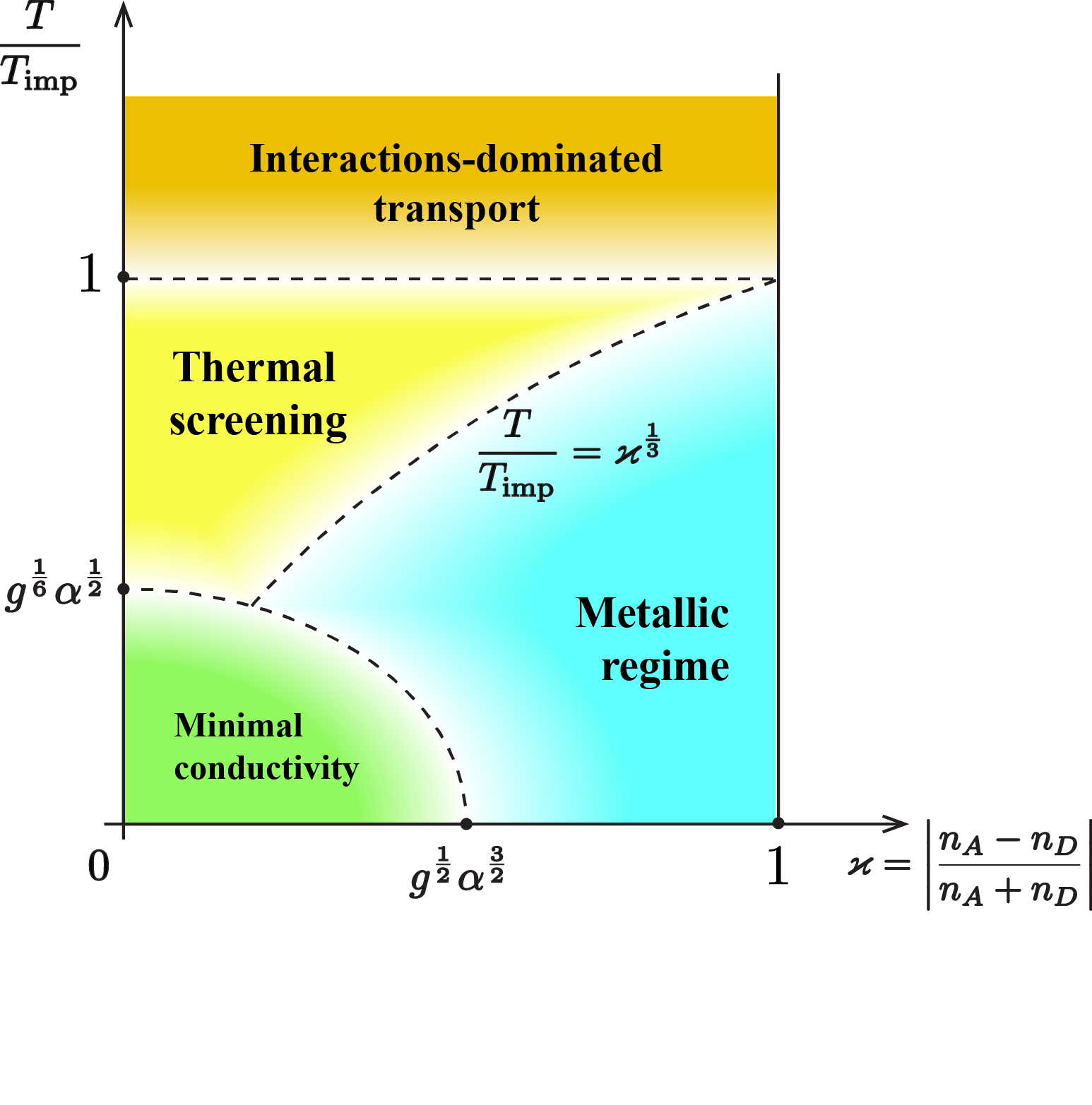
Figure 1: (Colour online) The temperature $T$ {in units $T_{\text{imp}}=[(n_{A}+n_{D})v^{3}/g]^{1/3}$} vs. the compensation parameter $\varkappa=\left|{n_{A}-n_{D}}\right|/({n_{A}+n_{D}})$ diagram for a Weyl semimetal with donor and acceptor impurities, where $n_{A}$ and $n_{D}$ are the concentrations of acceptor and donor impurities and $g$– the degeneracy of the Weyl point.

Currently it still remains to be investigated which of these phenomena and regimes of conduction can be realised in WSMs, under what conditions, and which of them display transport features specific to Weyl materials. Indeed, charged impurities, intrinsically present in realistic materials, lead to a finite chemical potential $\mu$ (measured from the Weyl point), making WSM similar to a usual metal in terms of transport properties at low temperatures $T\ll|\mu|$. Signatures of Weyl (Dirac) quasiparticles scattered by Coulomb impurities are expectedSarma et al. (2015) to be detectable at higher temperatures, $T\gg|\mu|$. However, the rate of quasiparticle scattering due to electron-electron interactions also grows with temperatureAbrikosov (1988); Hosur et al. (2012) and may prevail over the scattering on impurities.

Another question, that deserves investigation, is the dependency of the ac conductivity $\sigma(\omega)$ of a WSM on frequency $\omega$, as it can be used to directly measure the quasiparticle scattering time $\tau$ as a function of temperature or doping in the frequency range $\omega\sim\tau^{-1}$ and thus can provide information on the mechanisms of transport and the nature of disorder in a material.

In this paper we study the conductivity $\sigma(T,\omega,n_{A},n_{D})$ of a WSMs with donor (positively charged) and acceptor (negatively charged) impurities as a function of temperature $T$, frequency $\omega$, and the concentrations $n_{A}$ and $n_{D}$ of donors and acceptors.

Fig. 1 summarises different regimes of transport that can be achieved in a WSM by varying temperature and the concentrations of donors and acceptors. The frequency and temperature dependencies of conductivity in the “metallic regime” resemble those of a usual metal. The “interactions-dominated transport” is dominated by interactions and weakly depends on disorder. In the regime of “thermal screening” the conductivity and the screening of impurities is determined by electrons thermally excited from the valence to the conduction band, and the dc conductivity is strongly temperature-dependent, as predicted for small $\varkappa$ in Ref. Sarma et al., 2015. At low $T$ and $\varkappa=\left|{n_{A}-n_{D}}\right|/({n_{A}+n_{D}})$ strong fluctuations of the disorder potential lead to the formation of electron and hole puddles that determine the “minimal conductivity” introduced in Ref. Skinner, 2014.

Focussing on the disorder-dominated transport away from strong random-potential fluctuations (the “metallic” and “thermally screening” regions in Fig. 1), we calculate the conductivity $\sigma(T,\omega,n_{A},n_{D})$ explicitly and discuss the crossover behaviour between different regimes.

Our results apply both to Weyl semimetals and to Dirac semimetals, as the latter may be considered as Weyl semimetals with merging pairs of Weyl points.

The paper is organised as follows. In Sec. II we introduce the model for a Weyl semimetal with dopant impurities. Sec. III deals with relations between the concentration of dopants, chemical potential, and the fluctuations of the electron density. In Sec. IV we discuss the mechanisms of quasiparticle scattering and discuss the conditions under which the resistivity is disorder- and interactions-dominated. We evaluate the conductivity explicitly in Sec. V.1 and discuss the crossovers between various regimes of transport in Secs. V.2-V.4. In Sec. VI we summarise our results and discuss the experimental conditions necessary for realising each regime.

II Model

The Hamiltonian of long-wavelength quasiparticles in a WSM with charged impurities reads

$$\hat{\cal H} =\hat{\cal H}_{0}+\hat{\cal H}_{ee}+\hat{\cal H}_{\text{imp}},$$ (1a)

$$\hat{\cal H}_{0} =\int\hat{\psi}^{\dagger}({\bf r})v(\hat{\bm{\sigma}}\cdot\hat{\bf k})\>\hat{\psi}({\bf r})d^{3}{\bf r},$$ (1b)

$$\hat{\cal H}_{ee} =\int\hat{\psi}^{\dagger}({\bf r})\hat{\psi}^{\dagger}({\bf r}^{\prime})\frac{e^{2}}{\kappa|{\bf r}-{\bf r}^{\prime}|},\hat{\psi}({\bf r}^{\prime})\hat{\psi}({\bf r})\>d^{3}{\bf r}\,d^{3}{\bf r}^{\prime},$$ (1c)

$$\hat{\cal H}_{\text{imp}} =\sum_{i}\int\hat{\psi}^{\dagger}({\bf r})\frac{Z_{i}e^{2}}{\kappa|{\bf r}-{\bf r}_{i}|}\hat{\psi}({\bf r})\>d^{3}{\bf r},$$ (1d)

where $\hat{\cal H}_{0}$ is the Hamiltonian of free non-interacting Weyl fermions; $\hat{\psi}^{\dagger}({\bf r})$ and $\hat{\psi}({\bf r})$ are the fermion creation and annihilation operators, $v(\hat{\bm{\sigma}}\cdot\hat{\bf k})$ is the quasiparticle dispersion, with $\hat{\bf k}=-i\bf\nabla_{\bf r}$ being quasiparticle momentum, and $\hat{\bm{\sigma}}$– the pseudospin operator; $\hat{\cal H}_{ee}$ is the Hamiltonian of electron-electron interactions, $\varkappa$ being the dielectric constant; the operator $\hat{\cal H}_{\text{imp}}$ describes the interaction between electrons and charged impurities, located at random coordinates ${\bf r}_{i}$; $Z_{i}e$ is the charge of the $i$-th impurity. Throughout the paper we set $\hbar=1$. We consider two types of impurities: acceptors, with $Z_{i}=1$, and donors, with $Z_{i}=-1$.

Throughout the paper we assume for simplicity that the energies of bound states on the donor impurities are sufficiently high, and those on the acceptor impurities are sufficiently low, so that donors are always ionised and each acceptor always hosts an electron. In a realistic material, however, electron occupation numbers on dopant impurities may depend on the temperature and chemical potential. Our results can be easily generalised to this more realistic case; $n_{A}$ and $n_{D}$ should be understood then as the concentrations of impurities with charges $-e$ and $+e$ respectively, explicitly dependent on temperature and dopant concentrations.

Due to the fermion doubling theoremNielsen and Ninomiya (1985), Weyl quasiparticle dispersion is expected near an even number of points (Weyl points) in the first Brillouin zone. However, quasiparticle scattering between different Weyl points can be neglected due to the smoothness of the random potential created by the charged impurities under consideration and the due to long-range character of electron-electron interactions. For simplicity, we assume identical quasiparticles dispersions near all Weyl points and at the end of the calculation multiply the contribution of one point to the conductivity by a factor of $g$, that accounts for the number of Weyl and spin degeneracy.

The strength of electron-electron interactions is characterised by the “fine structure constant”

$$\alpha=\frac{e^{2}}{v\kappa},$$ (2)

which is assumed to be small, $\alpha\ll 1$, in this paper (for instance, inJay-Gerin et al. (1977); Liu et al. (2014b) $Cd_{3}As_{2}$ $\alpha\sim 0.05$). Throughout the paper we assume also, that the degeneracy $g$ is not very large, so that the condition

$$g\alpha\ll 1$$ (3)

is fulfilled.

III Charge-carrier density and impurity screening

In an undoped WSM the chemical potential is located at the Weyl point. Adding donor and acceptor impurities with different concentrations leads to a finite chemical potential $\mu$ (measured from the Weyl point) and an excess density $n(\mu)$ of electrons, as compared to the undoped sample. Charge neutrality of the material requires that

$$n_{D}-n_{A}=n(\mu,T),$$ (4)

where the excess electron density is given by

$$n(\mu,T) =g\sum_{\pm}\int\frac{d^{3}{\bf p}}{(2\pi)^{3}}\left[f_{0}(\pm v|{\bf p}|-\mu)-f_{0}(\pm v|{\bf p}|)\right]$$

$$=g\frac{\mu^{3}+\pi^{2}\mu T^{2}}{6\pi^{2}v^{3}},$$ (5)

with $f_{0}(\varepsilon)=(e^{\varepsilon/T}+1)^{-1}$ being the Fermi distribution function.

Fluctuations of electron density at low doping. Because impurities are located randomly, for very low densities $n(\mu,T)$ (i.e. for low $T$ and $\mu$) the distribution of electron charge displays strong relative spatial fluctuations and cannot be assumed uniform.

Indeed, as discussed in Refs. Skinner, 2014; Shklovskii and Efros, 1984, at small doping levels the fluctuations of the concentration of randomly located charged impurities lead to the formation of electron and hole puddles. In a WSM the characteristic depth of such puddles is given by the energy scaleSkinner (2014)

$$\Gamma\sim g^{-\frac{1}{6}}\alpha^{\frac{1}{2}}n_{\text{imp}}^{\frac{1}{3}}v,$$ (6)

where $n_{\text{imp}}\equiv n_{A}+n_{D}$ is the total concentration of the (donor and acceptor) impurities.

Unless the concentrations of donors and acceptors are nearly equal, the characteristic energy of the quasiparticles contributing to the conductivity can be estimated as $\varepsilon\sim\max(T,|\mu|)\gtrsim v(n_{\text{imp}}/g)^{\frac{1}{3}}$ [using Eqs. (4), (5), and $n_{D}-n_{A}\sim n_{\text{imp}}$] and significantly exceeds the scale $\Gamma$, Eq. (6). Thus, electron and hole puddles (studied in Ref. Skinner, 2014) can affect transport only in highly compensated materials, with nearly equal concentrations of donors and acceptors, $n_{A}\approx n_{D}$.

Using Eqs. (4), (5), and (6), we find that electron and hole puddles emerge only if

$$\left|\frac{n_{D}-n_{A}}{n_{D}+n_{A}}\right|\ll g^{\frac{1}{2}}\alpha^{\frac{3}{2}},$$ (7)

at low temperatures. Otherwise, relative fluctuations of electron distribution may be considered small.

The condition

$$\Gamma\lesssim\max(|\mu|,T)$$ (8)

determines the boundary of the “minimal conductivity” regime (studied in Ref. Skinner, 2014) in Fig. 1. Because of the large depth of electron and hole puddles in this regime, the conductivity is of the same order of magnitude in the entire “minimal conductivity” region. Outside of it, the fluctuations of the electron density are small, and the conductivity grows with temperature and chemical potential, as we find below.

Screening of impurities

Finite chemical potential $\mu$ or temperature $T$ lead to the screening of the charged impurities. Assuming the distribution of electrons is sufficiently homogeneous [i.e. the condition (7) does not hold], the screening radius $\lambda$ of the effective impurity potential

$$\phi({\bf r})=\frac{e^{2}}{\varkappa r}e^{-\frac{r}{\lambda}}$$ (9)

is given in the Thomas-Fermi approximation byAbrikosov (1988)

$$\lambda^{-2}=4\pi e^{2}n_{\mu}^{\prime}(\mu,T),$$ (10)

with the excess density $n(\mu,T)$ of electrons given by Eq. (5).

Using Eqs. (10) and (5), we obtain

$$\lambda^{-2}=\frac{2g\alpha}{\pi v^{2}}\left(\mu^{2}+\frac{\pi^{2}}{3}T^{2}\right).$$ (11)

The Thomas-Fermi approximation is justified for small values of the fine structure constant, $\alpha\ll 1$, assumed in this paper. This condition ensures that the screening radius (11) significantly exceeds the characteristic quasiparticle wavelength $\lambdabar=v/\max(T,|\mu|)$. Also, under this condition one can neglect the renormalisationSyzranov et al. (2015) of the low-energy quasiparticle properties from large momenta $k\gg\max(T,|\mu|)/v$.

Thermal screening vs. Fermi sea. Eq. (11) shows that at sufficiently high temperatures, $T\gg|\mu|$, the screening of the impurities is determined by electrons thermally excited from the valence to the conduction band and is independent of the concentrations of the impurities. In the opposite limit, $|\mu|\ll T$, the distribution of electron charge around an impurity is equivalent to that in a usual metalAbrikosov (1988). Thus, the boundary between the “thermal screening” and “metallic” regimes in Fig. 1 is given by the condition $\mu\sim T$, which, according to Eqs. 4 and 5, is equivalent to

$$T\sim v\left|\frac{n_{D}-n_{A}}{g}\right|^{\frac{1}{3}}.$$ (12)

IV Scattering times

Depending on the temperature and the concentrations of the dopants, resistivity in a WSM can be dominated by one of two quasiparticle scattering mechanisms. For sufficiently large amount of disorder, resistivity is expected to come from electron scattering on screened impurities. However, quasiparticles also can decay due to electron-electron interactions, which leads to a finite resistivity even in a disorder-free sampleAbrikosov and Beneslavskii (1971); Burkov et al. (2011).

Elastic scattering on screened impurities is characterised by the transport scattering time, in the Born approximation given by

$$\tau_{\text{tr}}^{-1}({\bf p})=\pi n_{\text{imp}}\rho\left(v|{\bf p}|\right)\int\frac{do}{4\pi}(1-\cos^{2}\theta)\left|u[2p\sin({\theta}/{2})]\right|^{2},$$ (13)

where $u({\bf k})=u(|{\bf k}|)$ is the Fourier-transform of the screened impurity potential, Eq. (9), and $\rho(\varepsilon)=\varepsilon^{2}/(2\pi v^{3})$ is the density of electron states at energy $\varepsilon$ (per spin and per Weyl point). For the screened Coulomb potential we find, using Eqs. (13) and (9),

$$\tau_{\text{tr}}^{-1}({\bf p})=\frac{2\pi\alpha^{2}n_{\text{imp}}v}{p^{2}}\left[\left(1+\frac{1}{2\lambda^{2}p^{2}}\right)\ln\left(1+4p^{2}\lambda^{2}\right)-2\right],$$ (14)

with the screening radius $\lambda(\mu,T)$ given by Eq. (11).

The characteristic momentum of the particles that contribute to the conductivity and the screening radius can be estimated as $p\sim\max(\mu,T)/v$ and $\lambda\sim(g\alpha)^{-\frac{1}{2}}v/\max(\mu,T)$ [Eq. (11)], respectively. Because of the large values of the parameter $p\lambda\sim(g\alpha)^{-\frac{1}{2}}\gg 1$, we neglect in what follows the dependence of the argument of the logarithm in Eq. (14) on the momentum $p$, $\ln\left(1+4p^{2}\lambda^{2}\right)\rightarrow\frac{1}{2}|\ln(g\alpha)|$.

Inelastic scattering. In the limit of an undoped material ($\mu\rightarrow 0$) the rate of scattering due to electron-electron interactionsAbrikosov and Beneslavskii (1971); Hosur et al. (2012) for a quasiparticle with momentum ${\bf p}$ is given by (up to logarithmic prefactors)

$$\tau^{-1}_{ee}({\bf p})\sim g\alpha^{2}v|{\bf p}|.$$ (15)

and decreases for a finite chemical potential.

Disorder- vs. interactions-dominated transport. Eqs. (14) and (15) show that the rate of inelastic scattering exceeds that of scattering on screened impurities only for quasiparticles with sufficiently high energies

$$\varepsilon\gtrsim T_{\text{imp}}\equiv v(n_{\text{imp}}/g)^{\frac{1}{3}},$$ (16)

where we have omitted the logarithmic factor of Eq. (14). Because the chemical potential satisfies the condition $\mu\lesssim v(n_{\text{imp}}/g)^{\frac{1}{3}}$, as follows from Eqs. (4) and (5), resistivity is dominated by the scattering due to electron-electron interactions only at sufficiently high temperatures $T\gg T_{\text{imp}}$, where $T=T_{\text{imp}}$ thus determines the boundary between the “interactions-dominated” and “thermal screening” regimes in Fig. 1.

Effective single-particle model.

In the rest of the paper we evaluate the conductivity $\sigma(T,\omega,n_{A},n_{D})$ of a doped WSM, focussing on the disorder-dominated transport with small fluctuations of the screened impurity potential, i.e. in the “thermal screening” and “metallic” regions in the diagram in Fig. 1. Also, we analyse the crossover of conduction to the other regimes on the boundaries of these regions.

The problem then can be considered effectively single-particle and described by the Hamiltonian

$$\hat{\cal H}^{\text{eff}} =\hat{\cal H}_{0}+\hat{\cal H}_{\text{imp}}^{\text{eff}}$$ (17)

$$\hat{\cal H}_{\text{imp}}^{\text{eff}} =\sum_{i}\int\hat{\psi}^{\dagger}({\bf r})\frac{e^{2}}{\kappa|{\bf r}-{\bf r}_{i}|}e^{-\frac{|{\bf r}-{\bf r}_{i}|}{\lambda}}\hat{\psi}({\bf r})\>d^{3}{\bf r},$$ (18)

where $\hat{\cal H}_{0}$ is the Hamiltonian of free Weyl fermions, and $\hat{\cal H}_{\text{imp}}$ describes the effective disorder potential, with the screening length $\lambda$ given by Eq. (11).

V Conductivity

V.1 General expressions

The conductivity of a disordered WSM is given by the Kubo-Greenwood formula

$$\sigma(\omega)=(2\pi\omega)^{-1}v^{2}g\int d\varepsilon\left[f_{0}(\varepsilon)-f_{0}(\varepsilon+\omega)\right]$$

$$\int d^{3}{\bf r}^{\prime}\>\>\mathrm{Tr}\left<\hat{\sigma}_{x}\hat{G}^{A}(\varepsilon+\omega,{\bf r},{\bf r}^{\prime})\hat{\sigma}_{x}\hat{G}^{R}(\varepsilon,{\bf r}^{\prime},{\bf r})\right>_{\text{dis}},$$ (19)

where $v\hat{\sigma}_{x}$ is the velocity operator along the $x$ axis; $\hat{G}^{A}(\varepsilon,{\bf r},{\bf r}^{\prime})$ and $\hat{G}^{R}(\varepsilon+\omega,{\bf r},{\bf r}^{\prime})$ are, respectively, the advanced and retarded Green’s functions, $2\times 2$ matrices in the pseudospin space, and $\langle\ldots\rangle$ denotes the averaging with respect to disorder realisations.

In the limit of weak disorder,

$$\tau_{\text{tr}}^{-1}[\max(\mu,T)/v]\ll\max(\mu,T),$$ (20)

the disorder-averaged correlator in Eq. (19) can be conveniently evaluated using a perturbative diagrammatic techniqueAbrikosov et al. (1975).

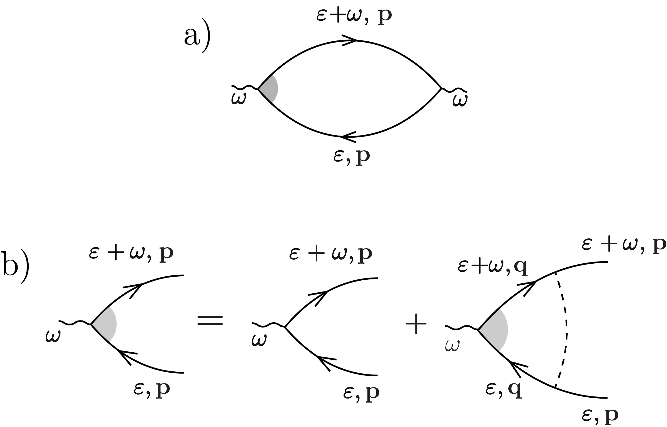
Figure 2: Diagrams for the conductivity. a) Current-current correlator. b) Dyson equation for the current vertex renormalised by disorder. Solid line is a fully disorder-averaged propagator of Weyl fermions.

The conductivity is given by the Drude contribution (shown diagrammatically in Fig. 2), which can be expressed in terms of the renormalised current vertex ${\bf J}({\bf p},\omega,\varepsilon)$ and the Fourier-transforms $\left<G^{A}(\varepsilon+\omega,{\bf p})\right>_{\text{dis}}$ and $\left<G^{R}(\varepsilon,{\bf p})\right>_{\text{dis}}$ of the disorder-averaged Green’s functions as

$$\sigma(\omega)=\frac{vg}{\omega}\int\frac{d\varepsilon}{2\pi}\>[f_{0}(\varepsilon)-f_{0}(\varepsilon+\omega)]$$

$$\int\frac{d^{3}{\bf p}}{(2\pi)^{3}}\mathrm{Tr}\left[\hat{J}_{x}({\bf p},\omega,\varepsilon)\left<G^{A}(\varepsilon+\omega,{\bf p})\right>_{\text{dis}}\right.$$

$$\left.\hat{\sigma}_{x}\left<G^{R}(\varepsilon,{\bf p})\right>_{\text{dis}}\right].$$ (21)

In this paper we focus on the range of frequencies $\omega$, that can be used to probe experimentally the quasiparticle scattering rate $\tau_{\text{tr}}^{-1}$ and are, therefore, smaller than the characteristic quasiparticle energy,

$$\omega\ll\max(T,\mu).$$ (22)

In the opposite limit, $\omega\gg\max(T,\mu)$, the WSM may be considered as a system of free Dirac fermions; the electron dynamics is collisionless [cf. the condition (20)] and the conductivity $\sigma(\omega)=\frac{ge^{2}}{24v}\omega$ (see, e.g., Ref. Hosur et al., 2012) is determined by the interband electromagnetic-field-induced transitions between the valence and the conduction bands.

Under the condition (22), Eq. (21) simplifies to (see Appendix A for details)

$$\sigma(\omega,\mu,T)=-\frac{e^{2}v^{2}g}{3\omega}\int\limits_{-\infty}^{\infty}\frac{\varepsilon^{2}d\varepsilon}{2\pi}\frac{f_{0}(\varepsilon+\omega)-f_{0}(\varepsilon)}{\tau_{\text{tr}}^{-1}(\varepsilon)-i\omega}.$$ (23)

From Eq. (23) we find, after some algebra (see Appendix B),

$$\sigma=-\frac{g}{i\omega}\frac{e^{2}T^{2}}{24\pi^{2}v}F\left[\frac{\alpha}{T}\left(\frac{2\pi n_{\text{imp}}v^{3}}{\omega}\right)^{\frac{1}{2}}\left|\ln{(g\alpha)}\right|^{\frac{1}{2}},\frac{\mu}{T},\frac{\omega}{T}\right],$$ (24)

where

$$F(\beta,\gamma,\Omega)=\frac{4}{3}(\pi^{2}+\Omega^{2})-4(i\beta^{2}-\gamma^{2})-4\gamma\Omega+\frac{2\sqrt{i}\beta^{3}}{\Omega}$$

$$\times\Bigg{[}\psi\left(\frac{1}{2}-\frac{i\gamma+\sqrt{i}\beta}{2\pi}\right)-\psi\left(\frac{1}{2}-\frac{i[\gamma-\Omega]+\sqrt{i}\beta}{2\pi}\right)$$

$$+\psi\left(\frac{1}{2}-\frac{i[\gamma-\Omega]-\sqrt{i}\beta}{2\pi}\right)-\psi\left(\frac{1}{2}-\frac{i\gamma-\sqrt{i}\beta}{2\pi}\right)$$

$$+2\pi i\bigg{(}\frac{1}{e^{i\sqrt{i}\beta-\gamma}+1}-\frac{1}{e^{i\sqrt{i}\beta-\gamma+\Omega}+1}\bigg{)}\Bigg{]}$$ (25)

with $\psi(x)$ being the digamma functionAbramowitz and Stegun (1972), and the ratio $\mu/T$ of the chemical potential to the temperature given by [as follows from Eqs. (4) and (5)]

$$\frac{\mu}{T}=\frac{2\pi}{\sqrt{3}}\sinh\left[\frac{1}{3}\operatorname{arcsinh}\left(\frac{9\sqrt{3}}{\pi}\frac{v^{3}}{g}\frac{n_{D}-n_{A}}{T^{3}}\right)\right].$$ (26)

Eqs. (24), (25), and (26) is our main result for the conductivity $\sigma(T,\omega,n_{A},N_{D})$ of a WSM as a function of temperature $T$, frequency $\omega$, and the impurity concentrations $n_{A}$ and $n_{D}$. In what immediately follows we analyse the limiting regimes of low temperatures, frequencies, and the amount of disorder and discuss the crossover behaviour between these regimes.

V.2 Metallic regime ($T\ll\mu$)

For low temperatures, $T\ll\mu\sim v\left|\frac{n_{D}-n_{A}}{g}\right|^{\frac{1}{3}}$, the transport properties of the WSM are similar to those of a usual metalAbrikosov (1988); conduction comes from low-energy excitations near the Fermi energy $\varepsilon_{F}=\left[6\pi^{2}v^{3}(n_{D}-n_{A})/g\right]^{\frac{1}{3}}\gg T$.

From Eqs. (24) and (25) we find the conductivity in this regime

$$\sigma\approx\left(\frac{g}{6\pi^{2}}\right)^{1/3}e^{2}v\frac{|n_{D}-n_{A}|^{2/3}}{\tau^{-1}_{tr}-i\omega}$$ (27)

with the transport scattering time given by

$$\tau^{-1}_{tr}=2\pi\left(\frac{g}{6\pi^{2}}\right)^{2/3}\frac{n_{\text{imp}}v}{|n_{D}-n_{A}|^{2/3}}\alpha^{2}|\ln({g\alpha})|.$$ (28)

The conductivity is weakly temperature-dependent and has the frequency dependency of a usual metalAbrikosov (1988), $\sigma\propto(\tau^{-1}_{tr}-i\omega)^{-1}$.

V.3 Regime of thermal screening, $\mu\ll T$

In the temperature interval

$$(|n_{D}-n_{A}|/g)^{\frac{1}{3}}v\ll T\ll(n_{\text{imp}}/g)^{\frac{1}{3}}v,$$ (29)

the chemical potential $\mu$ is small compared to $T$, and transport in the WSM is determined by electrons thermally excited from the vallence to conduction band.

From Eqs. (24) and (25) we find in this regime

$$\sigma(\omega,T)=\!\frac{ge^{2}T^{2}}{24\pi^{2}n_{\text{imp}}v^{4}}\!\begin{cases}\!\frac{14\pi^{3}T^{2}}{15\alpha^{2}|\ln({g\alpha})|},\!\!&\omega\ll\!\frac{\alpha^{2}|\ln(g\alpha)|n_{\text{imp}}v^{3}}{T^{2}},\\ \!\frac{4n_{\text{imp}}v^{3}\pi^{2}i}{3\omega},\!\!&\omega\gg\!\frac{\alpha^{2}|\ln(g\alpha)|n_{\text{imp}}v^{3}}{T^{2}}.\end{cases}$$ (30)

The limiting cases of low and high frequencies, Eq. (30), can be summarised by the interpolation formula

$$\sigma(\omega,T)=\frac{ge^{2}T^{2}}{18v}\frac{1}{\tau_{0}^{-1}-i\omega}$$ (31)

with the effective scattering time

$$\tau_{0}^{-1}=\frac{10}{7}\frac{\alpha^{2}n_{\text{imp}}v^{3}}{\pi T^{2}}|\ln(g\alpha)|.$$ (32)

Eqs. (31) and (32) resemble the usual-metal resultAbrikosov (1988) $\sigma(\omega)\propto[\tau^{-1}_{tr}-i\omega]^{-1}$ with an effective transport scattering time $\tau_{\text{tr}}=\tau_{0}$, Eq. (32). Indeed, Eqs. (31) and (32) can be understood as a result of the averaging of a metallic conductivity over an interval of energies $\varepsilon\sim T$ [cf. Eq. (23)]. Because the density of states and the transport scattering time [Eq. (14)] in a WSM are strongly energy-dependent, the effective scattering time and the prefactor in the averaged conductivity, Eq. (31), strongly depend on temperature.

For zero frequency, $\omega=0$, we reproduce the temperature dependence $\sigma\propto T^{4}$, obtained in Ref. Sarma et al., 2015 for a weakly-doped WSM (for sufficiently high temperatures).

At high frequencies, $T\gg\omega\gg\tau_{0}^{-1}$, the quasiparticle dynamics is collisionless, hence the conductivity is imaginary and decreases with frequency as $\sigma(\omega)\propto i/\omega$. We note, that this collisionless regime should be contrasted with the collisionless regime at $\omega\gg T$ with a real conductivityHosur et al. (2012) $\sigma(\omega)=\frac{ge^{2}}{24v}\omega$ that comes from the interband transitions.

Crossover to the interactions-dominated regime. For $T\sim T_{\text{imp}}\equiv[(n_{A}+n_{D})v^{3}/g]^{1/3}$ the dc conductivity

$$\sigma\sim\frac{T_{\text{imp}}}{\alpha}$$ (33)

matches the conductivityHosur et al. (2012); Burkov et al. (2011) $\sigma\sim T/\alpha$ of a disorder-free sample, because at $T\sim T_{\text{imp}}$ transport in a WSM crosses over from the disorder-dominated to the interactions-dominated regime.

V.4 dc Limit, $\omega\rightarrow 0$.

For very low frequencies,

$$\omega\ll\alpha^{2}\frac{n_{\text{imp}}v^{3}}{T^{2}}|\ln(g\alpha)|,$$ (34)

Eqs. (4) and (5) give

$$\begin{split}\sigma(\omega,T)&\approx\frac{ge^{2}T^{4}}{48\pi^{2}n_{\text{imp}}v^{3}\alpha^{2}|\ln(g\alpha)|}\Bigg{[}P_{4}\left(\frac{\mu}{T}\right)\\ &+\frac{i\omega T^{2}}{2\pi n_{\text{imp}}v^{3}\alpha^{2}|\ln(g\alpha)|}P_{6}\left(\frac{\mu}{T}\right)\\ &-\frac{\omega^{2}T^{4}}{2(2\pi n_{\text{imp}}\alpha^{2}|\ln g\alpha|)^{2}}P_{8}\left(\frac{\mu}{T}\right)\Bigg{]}\end{split}$$ (35)

where the ratio $\mu/T$ is given by Eq. (26), and

$$\begin{split}P_{4}(x)&=4x^{4}+8\pi^{2}x^{2}+\frac{28\pi^{4}}{15},\\ P_{6}(x)&=4x^{6}+20\pi^{2}x^{4}+28\pi^{4}x^{2}+\frac{121\pi^{6}}{21},\\ P_{8}(x)&=4\left(x^{8}+\frac{28\pi^{2}}{3}x^{6}+\frac{98\pi^{4}}{3}x^{4}+\frac{124\pi^{6}}{3}x^{2}+\frac{127\pi^{8}}{15}\right),\end{split}$$ (36)

As necessary, in the limits $\mu/T\ll 1$ and $\mu/T\gg 1$ Eq. (35) reproduces respectively Eq. (31) and (27) for $\omega=0$.

Crossover to the minimal conductivity. For $T=0$, $|n_{A}-n_{D}|\sim g^{\frac{1}{2}}\alpha^{\frac{3}{2}}n_{\text{imp}}$ and for $T\sim g^{\frac{1}{6}}\alpha^{\frac{1}{2}}v(n_{\text{imp}}/g)^{\frac{1}{3}}$, $n_{A}=n_{D}$, at the boundary of the “minimal conductivity” regime in Fig. 1, we find the value of the conductivity

$$\sigma_{\text{min}}\sim e^{2}(gn_{\text{imp}})^{\frac{1}{3}},$$ (37)

which, up to a prefactor of $g^{\frac{1}{3}}$ reproduces the minimal conductivity of a WSM obtained in Ref. Skinner, 2014. The conductivity is of the same order of magnitude, Eq. (37), in the entire “minimal conductivity” phase in Fig. 1, because the depth of electron and hole puddles in this regime significantly exceeds the temperature and the average chemical potential.

VI Discussion

We have studied conductivity of a Weyl semimetal with donor and acceptor impurities. Depending on the temperature $T$, and the concentrations $n_{A}$ and $n_{D}$ of acceptors and donors, the material may be in one of four regimes of conduction, that are summarised in Fig. 1. We have evaluated the conductivity $\sigma(T,\omega,n_{A},n_{D})$ explicitly in the “thermally screened” and “metallic” regimes and discussed the crossover behaviour to the other regimes.

Although experimental realisations of 3D Dirac materials are rather few and recent, it is possible to estimate the characteristic scales of temperatures, doping levels, and frequencies for various regimes of transport in Fig. 1, using the parameters of the quasiparticle spectrumLiu et al. (2014b); Neupane et al. (2014); Borisenko et al. (2014); Jeon et al. (2014) and the carrier densityJeon et al. (2014) in, e.g., the Dirac semimetal $\text{Cd}_{3}\text{As}_{2}$.

This material has the dielectric constantJay-Gerin et al. (1977) $\kappa\approx 36$, which for the Fermi velocity $v\sim 10^{6}\ \text{m}\cdot\text{s}^{-1}$ gives the effective fine structure constant $\alpha\sim 0.05$. Assuming the semimetal is not highly compensated, the concentrations of the charge carriers and Coulomb impurities are of the same order of magnitude, $|n_{D}-n_{A}|\sim n_{imp}\sim n$. For the charge carrier density $n\sim 10^{18}\,\text{cm}^{-3}$, reported in Ref. Jeon et al., 2014, both the chemical potential $\mu\approx 2000$K and the characteristic temperature $T_{\text{imp}}\sim n^{1/3}v\sim 10^{3}$K of the interactions-dominated scattering (see Fig. 1) significantly exceed the range of temperatures used in experiments. In terms of transport properties, such material is thus rather similar to a metal with the elastic scattering rate [Eq. (28)] $\tau_{\text{tr}}^{-1}\sim 10^{11}\ \text{Hz}\ (\sim 1\ \text{K})$. In order to observe significant frequency dependency of the conductivity, the frequency has to lie in the same range $\omega\sim 10^{11}\ \text{Hz}$ or higher. However, a weak frequency-dependent correction to the dc conductivity [see Eq. (35)] can be also observed at smaller frequencies.

In order to drive the material away from the metallic regime, the chemical potential has to be significantly reduced, which can by achieved by counterdoping, i.e. by introducing extra impurities in order to achieve nearly equal concentrations of donors and acceptors. For instance, achieving chemical potentials smaller than the room temperature requires the level of compensation $|n_{D}-n_{A}|/n_{\text{imp}}\lesssim 10^{-3}$. The conductivity in this “thermal screened” regime is strongly temperature-dependent, $\sigma\propto T^{2}/(CT^{-2}-i\omega)$ with the effective elastic scattering rate [Eq. (32)] at room temperature $\tau_{0}^{-1}=CT^{-2}\sim 10^{12}\ \text{Hz}$.

VII Acknowledgements

We are indebted to V.S. Khrapai for useful discussions and remarks on the manuscript. The work of SVS has been financially supported by the Alexander von Humboldt Foundation through the Feodor Lynen Research Fellowship and by the NSF grants DMR-1001240, DMR-1205303, PHY-1211914, and PHY-1125844. YaIR acknowledges financial support from the Ministry of Education and Science of the Russian Federation under the “Increase Competitiveness” Programme of NUST ”MISIS” (No. K2-2014-015), from the Russian Foundation for Basic Research under the project 14-02-00276, and from the Russian Science Support Foundation.

Appendix A Renormalised current vertex and conductivity

The renormalised current vertex, ${\bf J}(\omega,{\bf p},\varepsilon)$, satisfies the Dyson equation, shown diagrammatically in Fig. 2b,

$$\hat{\bf J}({\bf p},\omega,\varepsilon)=ev\hat{\bm{\sigma}}$$

$$+\int\frac{d^{3}{\bf q}}{(2\pi)^{3}}|u({\bf p}-{\bf q})|^{2}\hat{G}^{A}(\varepsilon+\omega,{\bf q})\hat{\bf J}({\bf q},\omega,\varepsilon)\hat{G}^{R}(\varepsilon,{\bf q}),$$ (38)

where ${\bf p}$ is the fermionic momentum, that goes in and out of the vertex ${\bf J}({\bf p},\omega)$ (Fig. 2b), $\varepsilon$ is the incoming fermionic energy, and $\omega$ is the frequency of the photon incoming in the vertex; $u({\bf k})$ is the Fourier-transform of the screened impurity potential; $ev\hat{\bm{\sigma}}$ is the bare (non-renormalised) current vertex;

$$\hat{G}^{R,A}(\varepsilon,{\bf p})=\frac{\varepsilon+v\hat{\bm{\sigma}}{\bf p}}{\left[\varepsilon\pm\frac{i}{2\tau({\bf p})}\right]^{2}-\left[vp\mp\frac{i}{2\tau_{1}({\bf p})}\right]^{2}}$$ (39)

are the disorder-averaged advanced and retarded Green’s functions where we have introduced the characteristic scattering rates

$$\tau^{-1}({\bf p})=\pi n_{\text{imp}}\rho\left(v|{\bf p}|\right)\int\frac{do}{4\pi}\left|u[2p\sin({\theta}/{2})]\right|^{2},$$ (40)

$$\tau_{1}^{-1}({\bf p})=\pi n_{\text{imp}}\rho\left(v|{\bf p}|\right)\int\frac{do}{4\pi}\left|u[2p\sin({\theta}/{2})]\right|^{2}\cos\theta,$$ (41)

where $\int do\ldots$ is the integration with respect to solid angle.

In the limit of weak disorder and small frequencies under consideration, only momenta ${\bf p}$ closeAbrikosov et al. (1975) to the mass shell $p=\varepsilon/v$ contribute to the response of quasiparticles with energy $\varepsilon$, encoded by the second line of Eq. (19). Accordingly, it is sufficient to consider the current vertex in Eq. (38) only with momenta ${\bf p}$ close to $\varepsilon/v$. Because of the smallness of the frequency $\omega$ the integration with respect to momenta ${\bf q}$ in Eq. (38) also can be assumed confined to a narrow shell of momenta near the surface $q=\varepsilon/v$.

Under these assumptions we look for the solution of the Dyson equation (38) in the form

$$\hat{\bf J}({\bf p},\omega,\varepsilon)=J_{1}(\omega)\>\hat{\bm{\sigma}}+J_{2}(\omega)\>v{\bf n}+J_{3}(\omega)\>v^{2}{{\bf n}(\hat{\bm{\sigma}}\cdot{\bf n})}$$ (42)

with $J_{1},\ldots,J_{3}$ being scalar functions and ${\bf n}={\bf p}/p$.

Plugging the ansatz (42) into the Dyson equation (38) for the current vertex and performing the momentum integration with $\omega\ll\varepsilon$ yields

$$J_{1}=ev+\frac{J_{1}+J_{2}+J_{3}}{2}\frac{\tau^{-1}_{\text{tr}}}{\tau^{-1}+\tau^{-1}_{1}-i\omega},$$ (43)

$$J_{2}=\frac{(J_{1}+J_{2}+J_{3})\tau^{-1}_{1}}{\tau^{-1}+\tau^{-1}_{1}-i\omega},$$ (44)

$$J_{3}=\frac{(J_{1}+J_{2}+J_{3})\left(\frac{1}{2}\tau^{-1}-\frac{3}{2}\tau^{-1}_{\text{tr}}\right)}{\tau^{-1}+{\tau_{1}}^{-1}-i\omega}.$$ (45)

From Eqs. (43)-(45) we find the sum

$$J_{1}+J_{2}+J_{3}=ev\frac{\tau^{-1}+\tau^{-1}_{1}-i\omega}{\tau^{-1}_{\text{tr}}-i\omega},$$ (46)

in terms of which the conductivity (21) in the limit $\omega\ll\varepsilon$ can be rewritten, using Eq. (39), as

$$\begin{split}\sigma(\omega)=-\frac{ge^{2}}{3\pi v}\int\limits_{-\infty}^{\infty}\frac{\varepsilon^{2}d\varepsilon}{2\pi}\frac{f_{0}(\varepsilon)-f_{0}(\varepsilon+\omega)}{\omega}\\ \frac{J_{1}(\omega)+J_{2}(\omega)+J_{3}(\omega)}{\tau^{-1}(\varepsilon)+\tau^{-1}_{1}(\varepsilon)-i\omega}.\end{split}$$ (47)

Using Eqs. (46) and (47) we arrive at Eq. (23).

Appendix B General expression for conductivity

In this Section we present a detailed derivation of expressions (24) and (25) from Eq. (23).

By introducing the notations

$$\gamma =\frac{\mu}{T},\ \ \Omega=\frac{\omega}{T}$$ (48)

$$a^{2} =\frac{2\pi\alpha^{2}n_{\text{imp}}v^{3}}{T^{2}\omega}\ln\left(1+4p^{2}\lambda^{2}\right)$$ (49)

$$\mathcal{D}_{x,\Omega}f(x) \equiv\frac{f(x)-f(x-\Omega)}{\Omega}$$ (50)

and neglecting the dependence of the logarithm on its argument, $\ln\left(1+4p^{2}\lambda^{2}\right)\rightarrow\frac{1}{2}|\ln(g\alpha)|$, Eq. (23) is reduced to Eq. (24) with

$$\begin{split}F(\beta,\gamma,\Omega)&=4\int\limits_{-\infty}^{\infty}\Big{(}\frac{1}{e^{x-\gamma-\Omega}+1}-\frac{1}{e^{x-\gamma}+1}\Big{)}\frac{dx\>x^{4}}{x^{2}+ia^{2}}\\ \equiv&-4\mathcal{D}_{\gamma,\Omega}\int\limits_{-\infty}^{\infty}\frac{x^{4}}{e^{x-\gamma}+1}\frac{dx}{x^{2}+ia^{2}}.\end{split}$$ (51)

To evaluate the integral (51) we split it into two parts: $F(a,\gamma)\equiv 4F_{I}(a,\gamma,\Omega)-4a^{4}F_{II}(a,\gamma,\Omega)$,

$$F_{I}(a,\gamma,\Omega)=\frac{\pi^{2}+\Omega^{2}}{3}-\gamma^{2}+ia^{2}+\gamma\Omega,$$ (52)

$$\begin{split}&F_{II}(a,\gamma,\Omega)=-\mathcal{D}_{\gamma,\Omega}\int_{-\infty}^{\infty}\frac{dx}{x^{2}+ia^{2}}\frac{1}{e^{x-\gamma}+1}\\ &=-\mathcal{D}_{\gamma,\Omega}\int\limits_{-\infty}^{\infty}f_{\gamma}(x)\,dx=-2\pi i\mathcal{D}_{\gamma,\Omega}\sum\limits_{n=0}^{\infty}\underset{x=x_{n}}{\text{res}}f_{\gamma}(x)\\ &-2\pi i\mathcal{D}_{\gamma,\Omega}\underset{x=i\sqrt{i}a}{\text{res}}f_{\gamma}(x),\end{split}$$ (53)

where $\sqrt{i}=\frac{1+i}{\sqrt{2}}$.

The residue of the function $f(x)$ at $x=x_{n}=\gamma+i\pi(2n+1)$, $n=0,1,2,\ldots$ is given by

$$\begin{split}&\underset{x=x_{n}}{\text{res}}f_{\gamma}(x)=-\frac{1}{x_{n}^{2}+ia^{2}}\\ &=\frac{1}{2i\sqrt{i}a}\left[\frac{1}{x_{n}+i\sqrt{i}a}-\frac{1}{x_{n}-i\sqrt{i}a}\right],\end{split}$$ (54)

the residue at $x=i\sqrt{i}a$–

$$\underset{x=i\sqrt{i}a}{\text{res}}f_{\gamma}(x)=\frac{1}{2i\sqrt{i}a}\frac{1}{e^{i\sqrt{i}a-\gamma}+1}.$$ (55)

Using Eqs. (53), (54), and (55), we obtain

$$F_{II}(a,\gamma,\Omega)=-\mathcal{D}_{\gamma,\Omega}\Bigg{(}\frac{\sqrt{i}}{2a}\sum\limits_{n=0}^{\infty}\left[\frac{1}{n+\frac{1}{2}-\frac{\sqrt{i}a}{2\pi}-\frac{i\gamma}{2\pi}}\right.$$

$$\left.-\frac{1}{n+\frac{1}{2}+\frac{\sqrt{i}a}{2\pi}-\frac{i\gamma}{2\pi}}\right]+\frac{\pi}{\sqrt{i}a}\frac{1}{e^{i\sqrt{i}a-\gamma}+1}\Bigg{)}.$$ (56)

Using Eqs. (52) and (53) and the definition of the digamma functionAbramowitz and Stegun (1972),

$$\psi(z)=\sum\limits_{0}^{\infty}\left(\frac{1}{n+1}-\frac{1}{z+a}\right)-C,$$ (57)

with $C$ being the Euler constant, we arrive at Eq. (25).

References

- Burkov and Balents (2011) A. A. Burkov and L. Balents, Phys. Rev. Lett. 107, 127205 (2011).
- Wan et al. (2011) X. Wan, A. M. Turner, A. Vishwanath, and S. Y. Savrasov, Phys. Rev. B 83, 205101 (2011).
- Xu et al. (2015) S.-Y. Xu, C. Liu, S. K. Kushwaha, R. Sankar, J. W. Krizan, I. Belopolski, M. Neupane, G. Bian, N. Alidoust, T.-R. Chang, et al., Observation of fermi arc surface states in a topological metal: A new type of 2d electron gas beyond topological insulators (2015), arXiv:1501.01249.
- Lv et al. (2015) B. Q. Lv, H. M. Weng, B. B. Fu, X. P. Wang, H. Miao, J. Ma, P. Richard, X. C. Huang, L. X. Zhao, G. F. Chen, et al., Discovery of weyl semimetal TaAs (2015), arXiv:1502.04684.
- Liu et al. (2014a) Z. K. Liu, B. Zhou, Y. Zhang, Z. J. Wang, H. M. Weng, D. Prabhakaran, S.-K. Mo, Z. X. Shen, Z. Fang, X. Dai, et al., Science 343, 865 (2014a).
- Neupane et al. (2014) M. Neupane, S.-Y. Xu, R. Sankar, N. Alidoust, G. Bian, C. Liu, I. Belopolski, T.-R. Chang, H.-T. Jeng, H. Lin, et al., Nature Comm. 5, 3786 (2014).
- Borisenko et al. (2014) S. Borisenko, Q. Gibson, D. Evtushinsky, V. Zabolotnyy, B. Büchner, and R. J. Cava, Phys. Rev. Lett. 113, 027603 (2014).
- Jeon et al. (2014) S. Jeon, B. B. Zhou, A. Gyenis, B. E. Feldman, I. Kimchi, A. C. Potter, Q. D. Gibson, R. J. Cava, A. Vishwanath, and A. Yazdani (2014), arXiv:1403.3446.
- Liu et al. (2014b) Z. K. Liu, J. Jiang, B. Zhou, Z. J.Wang, Y. Zhang, H. M.Weng, D. Prabhakaran, S.-K. Mo, H. Peng, P. Dudin, et al., Nature Mat. 13, 677 (2014b).
- Ryu et al. (2010) S. Ryu, A. Schnyder, A. Furusaki, and A. Ludwig, New J. Phys. 12, 065010 (2010).
- Fradkin (1986a) E. Fradkin, Phys. Rev. B 33, 3263 (1986a).
- Fradkin (1986b) E. Fradkin, Phys. Rev. Lett. 33, 3257 (1986b).
- Goswami and Chakravarty (2011) P. Goswami and S. Chakravarty, Phys. Rev. Lett. 107, 196803 (2011).
- Syzranov et al. (2014) S. V. Syzranov, L. Radzihovsky, and V. Gurarie (2014), arXiv:1402.3737.
- Sbierski et al. (2014) B. Sbierski, G. Pohl, E. J. Bergholtz, and P. W. Brouwer, Phys. Rev. Lett. 113, 026602 (2014).
- Moon and Kim (2014) E.-G. Moon and Y. B. Kim (2014), arXiv:1409.0573.
- Kobayashi et al. (2014) K. Kobayashi, T. Ohtsuki, K.-I. Imura, and I. F. Herbut, Phys. Rev. Lett. 112, 016402 (2014).
- Syzranov et al. (2015) S. Syzranov, V. Gurarie, and L. Radzihovsky, Phys. Rev. B 91, 035133 (2015).
- Dotsenko and Dotsenko (1983) V. S. Dotsenko and V. S. Dotsenko, Adv. Phys. 32, 129 (1983).
- Ludwig et al. (1994) A. W. W. Ludwig, M. P. A. Fisher, R. Shankar, and G. Grinstein, Phys. Rev. B 50, 7526 (1994).
- Nersesyan et al. (1994) A. A. Nersesyan, A. M. Tsvelik, and F. Wenger, Phys. Rev. Lett. 72, 2628 (1994).
- Aleiner and Efetov (2006) I. L. Aleiner and K. B. Efetov, Phys. Rev. Lett. 97, 236801 (2006).
- Ostrovsky et al. (2006) P. M. Ostrovsky, I. V. Gornyi, and A. D. Mirlin, Phys. Rev. B 74, 235443 (2006).
- Roy and Sarma (2014) B. Roy and S. D. Sarma, Phys. Rev. B 90, 241112(R) (2014).
- Skinner (2014) B. Skinner, Phys. Rev. B 90, 060202(R) (2014).
- Burkov et al. (2011) A. A. Burkov, M. D. Hook, and L. Balents, Phys. Rev. B 84, 235126 (2011).
- Ominato and Koshino (2015) Y. Ominato and M. Koshino, Phys. Rev. B 91 (2015).
- Sarma et al. (2015) S. D. Sarma, E. H. Hwang, and H. Min, Phys. Rev. B 91, 035201 (2015).
- Lundgren et al. (2014) R. Lundgren, P. Laurell, and G. A. Fiete, Phys. Rev. B 90, 165115 (2014).
- Ramakrishnan et al. (2015) N. Ramakrishnan, M. Milletari, and S. Adam (2015), arXiv:1501.03815.
- Abrikosov (1988) A. A. Abrikosov, Fundamentals of the Theory of Metals (Elsevier, North-Holland, 1988).
- Hosur et al. (2012) P. Hosur, S. A. Parameswaran, and A. Vishwanath, Phys. Rev. Lett. 108, 046602 (2012).
- Nielsen and Ninomiya (1985) H. B. Nielsen and M. Ninomiya, Nuclear Physics B 185, 20 (1985).
- Jay-Gerin et al. (1977) J.-P. Jay-Gerin, M. J. Aubin, and L. G. Caron, Solid State Comm. 21, 771 (1977).
- Shklovskii and Efros (1984) B. I. Shklovskii and A. L. Efros, Electronic properties of doped semiconductors (Springer, Heidelberg, 1984).
- Abrikosov and Beneslavskii (1971) A. A. Abrikosov and S. D. Beneslavskii, Sov. Phys. JETP 32, 699 (1971).
- Abrikosov et al. (1975) A. A. Abrikosov, L. P. Gorkov, and I. E. Dzyaloshinski, Methods of Quantum Field Theory in Statistical Physics (Dover, New York, 1975).
- Abramowitz and Stegun (1972) M. Abramowitz and I. Stegun, Handbook of Mathematical Functions (Dover Publications, New York, 1972).