Non-extended phase space thermodynamics of Lovelock AdS black holes in grand canonical ensemble

Abstract

Recently, extended phase space thermodynamics of Lovelock AdS black holes has been of great interest. To provide insight from a different perspective and gain a unified phase transition picture, non-extended phase space thermodynamics of $(n+1)$-dimensional charged topological Lovelock AdS black holes is investigated detailedly in the grand canonical ensemble. Specifically, the specific heat at constant electric potential is calculated and phase transition in the grand canonical ensemble is discussed. To probe the impact of the various parameters, we utilize the control variate method and solve the phase transition condition equation numerically for the case $k=1,-1$. There are two critical points for the case $n=6,k=1$ while there is only one for other cases. For $k=0$, there exists no phase transition point. To figure out the nature of phase transition in the grand canonical ensemble, we carry out an analytic check of the analog form of Ehrenfest equations proposed by Banerjee et al. It is shown that Lovelock AdS black holes in the grand canonical ensemble undergo a second order phase transition. To examine the phase structure in the grand canonical ensemble, we utilize the thermodynamic geometry method and calculate both the Weinhold metric and Ruppeiner metric. It is shown that for both analytic and graphical results that the divergence structure of the Ruppeiner scalar curvature coincides with that of the specific heat. Our research provides one more example that Ruppeiner metric serves as a wonderful tool to probe the phase structures of black holes.

I Introduction

In our recent paper Wenbiao3 , $P-V$ criticality of topological AdS black holes in Lovelock-Born-Infeld gravity has been investigated in the extended phase space and some unique phenomena have been found. It was shown that $P-V$ criticality exists not only for the spherical topology but also for $k=-1$. This result is really intriguing that it has attracted further investigation Belhaj95 - Dolan99 . On the other hand, it would also be interesting to probe this issue in the non-extended phase space to search for some more unique characteristics due to Lovelock gravity. Lovelock gravity Lovelock is a particular higher curvature gravity theory which successfully solves the problem of fourth order field equations and ghost. In Lovelock gravity, the field equation is only second order and the quantization is free of ghosts Boulware . Both the black holes and their thermodynamics in Lovelock gravity Dehghani1 -Amirabi have attracted considerable attention. Concerning the thermodynamics of Lovelock black holes in the non-extended phase space, some efforts have been made. Topological black hole solutions in Lovelock-Born-Infeld gravity were proposed in Ref. Dehghani1 . Both the thermodynamics of asymptotically AdS rotating black branes with flat horizon and asymptotically flat black holes for $k=1$ were detailedly investigated there. For charged topological AdS black holes, Ref. Dehghani1 presented the expression of the temperature. Ref. Decheng4 ; Decheng2 further studied their entropy and specific heat at constant charge. Ref. Lala2 studied their specific heat and critical exponents in the canonical ensemble. The above research was carried out in the canonical ensemble, leaving the grand canonical ensemble unexplored. In this paper, we would like to complete the phase transition research of Lovelock charged topological AdS black holes in the grand canonical ensemble.

In traditional thermodynamics, one can utilize Clausius-Clapeyron-Ehrenfest’s equations to probe the nature of phase transitions. The Clausius-Clapeyron equation holds for a first order phase transition while Ehrenfest’s equations are satisfied for a second order phase transition. Recently, Banerjee et al. introduced a novel Ehrenfest scheme to investigate phase transitions of black holes in the grand canonical ensemble Banerjee1 -Banerjee6 . We utilized this scheme in the case of charged topological black hole in Hořava-Lifshitz gravity Wenbiao2 and also generalized it to the extended phase space Wenbiao1 -Wenbiao4 . Ref. Jiliangjing further generalized it to the full phase space. The original Ehrenfest equations in traditional thermodynamics were utilized in the extended space of black holes in Lovelock-Born-Infeld gravity to study the nature of phase transition at the critical point Belhaj95 . However, in this paper, we would like to utilize the analog form of Ehrenfest scheme proposed by Banerjee et al. to investigate the nature of phase transition points of Lovelock AdS black holes in the grand canonical ensemble.

Different from the traditional thermodynamic method, thermodynamic geometry has served as an alternative way to investigate phase transitions of black holes. The well-known examples are Weinhold geometry Weinhold and Ruppeiner geometry Ruppeiner . Weinhold defined metric structure in the energy representation as $g_{i,j}^{W}=\partial_{i}\partial_{j}M(U,N^{a})$. Here, $U$ is the internal energy $U$ while $N^{a}$ represents the extensive thermodynamic variables. Ruppeiner proposed metric structure as the Hessian of the entropy. Namely, $g_{i,j}^{R}=-\partial_{i}\partial_{j}S(U,N^{a})$. Recently, Quevedo et al. Quevedo2 proposed another thermodynamic geometry method named as geometrothermodynamics (GTD). For its profound physical meaning, Ruppeiner’s metric has been applied to investigate various thermodynamic systems including black holes. For a nice review of Ruppeiner geometry, see Ref. Ruppeiner2 . For recent papers, see Ref. Tharanath - Niu . However, thermodynamic geometry of Lovelock AdS black holes in the grand canonical ensemble is still absent in literature. In this paper, we would like to explore the Ruppeiner geometry of $(n+1)$-dimensional topological AdS black holes in Lovelock gravity in the grand canonical ensemble .

In Sec. II, the thermodynamics of charged topological AdS black holes in Lovelock-Born-Infeld gravity will be briefly reviewed and the phase transition in the grand canonical ensemble will be investigated in detail. To probe the nature of phase transition in the grand canonical ensemble, an analytic check of the analog form of Ehrenfest equations will be carried out in Sec. III. In Sec. IV, thermodynamic geometry will be studied to examine the phase structure of topological AdS black holes. Concluding remarks will be presented in Sec. V.

II Phase transition in the grand canonical ensemble

The action of third order Lovelock-Born-Infeld gravity readsDehghani1

$$I_{G}=\frac{1}{16\pi}\int d^{n+1}x\sqrt{-g}\big{(}-2\Lambda+\mathcal{L}_{1}+\alpha_{2}\mathcal{L}_{2}+\alpha_{3}\mathcal{L}_{3}+L(F)\big{)},$$ (1)

where

$$\mathcal{L}_{1} = R,$$ (2)

$$\mathcal{L}_{2} = R_{\mu\nu\gamma\delta}R^{\mu\nu\gamma\delta}-4R_{\mu\nu}R^{\mu\nu}+R^{2},$$ (3)

$$\mathcal{L}_{3} = 2R^{\mu\nu\sigma\kappa}R_{\sigma\kappa\rho\tau}R^{\rho\tau}_{\;\;\;\;\mu\nu}+8R^{\mu\nu}_{\;\;\;\;\sigma\rho}R^{\sigma\kappa}_{\;\;\;\;\nu\tau}R^{\rho\tau}_{\;\;\;\;\mu\kappa}+24R^{\mu\nu\sigma\kappa}R_{\sigma\kappa\nu\rho}R^{\rho}_{\;\;\mu}$$ (4)

$$+3RR^{\mu\nu\sigma\kappa}R_{\sigma\kappa\mu\nu}+24R^{\mu\nu\sigma\kappa}R_{\sigma\mu}R_{\kappa\nu}+16R^{\mu\nu}R_{\nu\sigma}R^{\sigma}_{\;\;\mu}-12RR^{\mu\nu}R_{\mu\nu}+R^{3},$$

$$L(F) = 4\beta^{2}\left(1-\sqrt{1+\frac{F^{2}}{2\beta^{2}}}\right).$$ (5)

$\beta$, $\alpha_{2}$ and $\alpha_{3}$ are Born-Infeld parameter, the second and third order Lovelock coefficients respectively. $L(F)$ denotes the Born-Infeld Lagrangian with $F_{\mu\nu}=\partial_{\mu}A_{\nu}-\partial_{\nu}A_{\mu}$, where $A_{\mu}$ is electromagnetic vector. The $(n+1)$-dimensional static solution was derived in Ref. Dehghani1 as

$$ds^{2}=-f(r)dt^{2}+\frac{dr^{2}}{f(r)}+r^{2}d\Omega^{2},$$ (6)

where

$$f(r) = k+\frac{r^{2}}{\alpha}(1-g(r)^{1/3}),$$ (7)

$$g(r) = 1+\frac{3\alpha m}{r^{n}}-\frac{12\alpha\beta^{2}}{n(n-1)}\Big{[}1-\sqrt{1+\eta}-\frac{\Lambda}{2\beta^{2}}+\frac{(n-1)\eta}{(n-2)}\digamma(\eta)\Big{]}.$$ (8)

$k$ and $m$ are parameters related to the curvature of hypersurface and the mass respectively. $d\Omega^{2}$ denotes the line element of $(n-1)$-dimensional hypersurface with constant curvature $(n-1)(n-2)k$ and $\digamma(\eta)$ denotes the hypergeometric function as follow

$$\digamma(\eta)=\,_{2}F_{1}\Big{(}\Big{[}\frac{1}{2},\frac{n-2}{2n-2}\Big{]},\Big{[}\frac{3n-4}{2n-2}\Big{]},-\eta\Big{)},$$ (9)

where

$$\eta=\frac{(n-1)(n-2)q^{2}}{2\beta^{2}r^{2n-2}}.$$ (10)

Note that the above solution was derived for the special case that

$$\alpha_{2} = \frac{\alpha}{(n-2)(n-3)},$$ (11)

$$\alpha_{3} = \frac{\alpha^{2}}{72{n-2\choose 4}}.$$ (12)

When $\beta\rightarrow\infty$, the Born-Infeld Lagrangian reduces to the Maxwell form and the solutions become Lovelock AdS black holes. To concentrate on the effects of the third order Lovelock gravity, we will mainly consider Lovelock AdS black holes in this paper.

When $\beta\rightarrow\infty$, one can obtain

$$g(r)\rightarrow 1+\frac{3\alpha m}{r^{n}}+\frac{6\alpha\Lambda}{n(n-1)}-\frac{3\alpha q^{2}}{r^{2n-2}}.$$ (13)

The horizon radius $r_{+}$ can be derived from the largest root of the equation $f(r)=0$. One can express $m$ in the function of $r_{+}$ as

$$m=\frac{3n(n-1)q^{2}r_{+}^{8}+r_{+}^{2n}\left[kn(n-1)(3r_{+}^{4}+3kr_{+}^{2}\alpha+k^{2}\alpha^{2})-6r_{+}^{6}\Lambda\right]}{3n(n-1)r_{+}^{n+6}}.$$ (14)

Then the mass of $(n+1)$-dimensional topological AdS black holes can be derived as

$$M=\frac{(n-1)\Sigma_{k}}{16\pi}m=\frac{\Sigma_{k}}{48n\pi r_{+}^{n+6}}\left\{3n(n-1)q^{2}r_{+}^{8}+r_{+}^{2n}\left[kn(n-1)(3r_{+}^{4}+3kr_{+}^{2}\alpha+k^{2}\alpha^{2})-6r_{+}^{6}\Lambda\right]\right\},$$ (15)

where $\Sigma_{k}$ denotes the volume of the $(n-1)$-dimensional hypersurface. The Hawking temperature has been derived in Ref. Dehghani1 as

$$T=\frac{(n-1)k[3(n-2)r_{+}^{4}+3(n-4)k\alpha r_{+}^{2}+(n-6)k^{2}\alpha^{2}]+12r_{+}^{6}\beta^{2}(1-\sqrt{1+\eta_{+}}\,)-6\Lambda r_{+}^{6}}{12\pi(n-1)r_{+}(r_{+}^{2}+k\alpha)^{2}}.$$ (16)

Taking the limit $\beta\rightarrow\infty$, Eq. (16) reduces to

$$T=\frac{(n-1)k[3(n-2)r_{+}^{4}+3(n-4)k\alpha r_{+}^{2}+(n-6)k^{2}\alpha^{2}]-6\Lambda r_{+}^{6}-3(n-2)(n-1)q^{2}r_{+}^{8-2n}}{12\pi(n-1)r_{+}(r_{+}^{2}+k\alpha)^{2}}.$$ (17)

In the non-extended phase space, the first law of thermodynamics reads

$$dM=TdS+\Phi dQ.$$ (18)

So the entropy can be derived as

$$S=\int^{r_{+}}_{0}\frac{1}{T}\left(\frac{\partial M}{\partial r_{+}}\right)dr=\frac{\Sigma_{k}(n-1)r_{+}^{n-5}}{4}\left(\frac{r_{+}^{4}}{n-1}+\frac{2kr_{+}^{2}\alpha}{n-3}+\frac{k^{2}\alpha^{2}}{n-5}\right).$$ (19)

The above result is derived for $n>5$ while the integration is divergent for $n\leqslant 5$. The charge $Q$ is related to the parameter $q$ by

$$Q=\frac{\Sigma_{k}}{4\pi}\sqrt{\frac{(n-1)(n-2)}{2}}q.$$ (20)

Then the expression of the mass can be reorganized as

$$M=\frac{96n\pi^{2}Q^{2}r_{+}^{8}+r_{+}^{2n}(n-2)\left[kn(n-1)(3r_{+}^{4}+3kr_{+}^{2}\alpha+k^{2}\alpha^{2})-6r_{+}^{6}\Lambda\right]\Sigma_{k}^{2}}{48n(n-2)\pi r_{+}^{n+6}\Sigma_{k}}.$$ (21)

Utilizing Eqs. (18) and (21), the electric potential can be calculated as

$$\Phi=\Big{(}\frac{\partial M}{\partial Q}\Big{)}_{S}=\frac{4\pi Q}{(n-2)r_{+}^{n-2}\Sigma_{k}}.$$ (22)

To study the phase transition in the grand canonical ensemble, it is more convenient to express the mass into the function of the electric potential $\Phi$ as follows

$$M = \frac{6n(n-2)^{2}\Phi^{2}r_{+}^{2n+4}\Sigma_{k}^{3}+r_{+}^{2n}(n-2)\Sigma_{k}\left[kn(n-1)(3r_{+}^{4}+3kr_{+}^{2}\alpha+k^{2}\alpha^{2})-6r_{+}^{6}\Lambda\right]}{48n(n-2)\pi r_{+}^{n+6}},$$ (23)

$$T = \frac{(n-1)k[3(n-2)r_{+}^{4}+3(n-4)k\alpha r_{+}^{2}+(n-6)k^{2}\alpha^{2}]-6\Lambda r_{+}^{6}-6(n-2)^{2}\Phi^{2}r_{+}^{4}}{12\pi(n-1)r_{+}(r_{+}^{2}+k\alpha)^{2}}.$$ (24)

The specific heat at constant electric potential can be obtained as

$$C_{\Phi}=T\Big{(}\frac{\partial S}{\partial T}\Big{)}_{\Phi}=\frac{A(r_{+},\Phi)}{B(r_{+},\Phi)},$$ (25)

where

$$A(r_{+},\Phi) = (n-1)r_{+}^{n-5}(r_{+}^{2}+k\alpha)^{3}\Sigma_{k}$$ (26)

$$\times\left[3k(n-2)(n-1)r_{+}^{4}+3k^{2}(n-4)(n-1)r_{+}^{2}\alpha+k^{3}(n-6)(n-1)\alpha^{2}-6r_{+}^{6}\Lambda-6(n-2)^{2}r_{+}^{4}\Phi^{2}\right],$$

$$B(r_{+},\Phi) = -24\Lambda r_{+}^{8}-12\left[k(2+n^{2}-3n+10\alpha\Lambda)-2(n-2)^{2}\Phi^{2}\right]r_{+}^{6}+72k\alpha r_{+}^{4}\left[k(n-1)-(n-2)^{2}\Phi^{2}\right]$$ (27)

$$-8k^{3}(n-9)(n-1)\alpha^{2}r_{+}^{2}-4k^{4}(n-6)(n-1)\alpha^{3}.$$

One can easily draw the conclusion that the specific heat at constant electric potential may diverge when

$$B(r_{+},\Phi)=0,$$ (28)

implying the existence of phase transition.

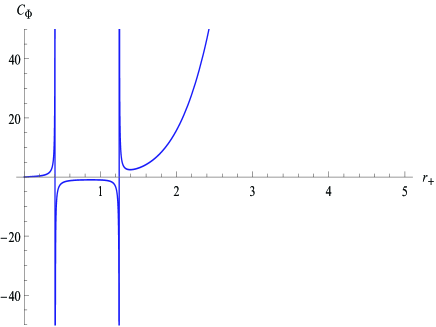
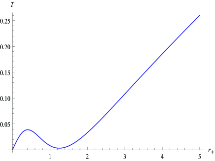
Figure 1: (a) $C_{\Phi}$ vs. $r_{+}$ for $k=1,n=6,\alpha=1,\Phi=1,\Lambda=-2$ (b) $T$ vs. $r_{+}$ for $k=1,n=6,\alpha=1,\Phi=1,\Lambda=-2$

The above equation can be solved numerically and the results for $k=1,-1$ are presented in Table 1-2 respectively, where the impact of the various parameters are studied thoroughly via control variate method. It is quite interesting to note that there are two critical points for the case $n=6,k=1$ while there is only one for other cases. And the distance between the two phase transition points becomes larger with the increasing of $\Lambda$ and $\Phi$ while it first becomes larger then becomes smaller with the increasing of $\alpha$. The case $n=6,k=1$ is shown graphically in Fig.1. Both the behaviors of the specific heat and Hawking temperature are depicted. It is easy to find that the two phase transition points where the specific heat diverges are physical for the Hawking temperature is positive. The black holes can be divided into three phases. Namely, small stable ($C_{\Phi}>0$) black hole, medium unstable ($C_{\Phi}<0$) black hole and large stable ($C_{\Phi}>0$) black hole. For a more comprehensive picture, we also plot the three-dimensional figure for the case $n=6,k=1$ in Fig.2 and for the case $n=6,k=-1$ in Fig.3.

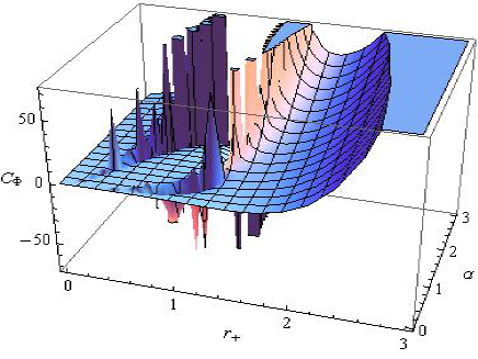
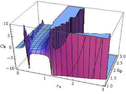
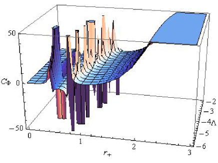
Figure 2: (a) $C_{\Phi}$ vs. $r_{+}$ for $k=1,n=6,\Phi=1,\Lambda=-2$ (b) $T$ vs. $r_{+}$ for $k=1,n=6,\alpha=1,\Lambda=-2$ (c) $C_{\Phi}$ vs. $r_{+}$ for $k=1,n=6,\alpha=1,\Phi=1$

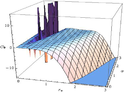
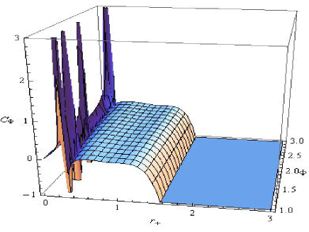
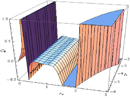
Figure 3: (a) $C_{\Phi}$ vs. $r_{+}$ for $k=-1,n=6,\Phi=1,\Lambda=-2$ (b) $T$ vs. $r_{+}$ for $k=-1,n=6,\alpha=1,\Lambda=-2$ (c) $C_{\Phi}$ vs. $r_{+}$ for $k=-1,n=6,\alpha=1,\Phi=1$

The case $k=0$ is quite simple. When $k=0$, Eq. (27) can be simplified as

$$B(r_{+},\Phi)=-24\Lambda r_{+}^{8}+24(n-2)^{2}\Phi^{2}>0.$$ (29)

So there exists no phase transition for $k=0$.

Table 1: The location of phase transition points for $k=1$

  $n$ $\alpha$ $\Phi$ $\Lambda$ $r_{+1}$ $r_{+2}$ 6 1 1 -2 0.406 1.248 6 1 1 -4 0.420 0.964 6 1 1 -6 0.440 0.794 6 0.5 1 -2 0.283 1.076 6 2 1 -2 0.595 1.363 6 1 2 -2 0.169 1.592 6 1 3 -2 0.110 1.666 7 1 1 -2 1.503 - 8 1 1 -2 1.680 - 9 1 1 -2 1.812 -  

Table 2: The location of phase transition points for $k=-1$

  $n$ $\alpha$ $\Phi$ $\Lambda$ $r_{+}$ 6 1 1 -2 0.279 6 1 1 -4 0.281 6 1 1 -6 0.282 6 0.5 1 -2 0.197 6 2 1 -2 0.397 6 1 2 -2 0.155 6 1 3 -2 0.106 7 1 1 -2 0.353 8 1 1 -2 0.374 9 1 1 -2 0.386  

III The nature of phase transition in the grand canonical ensemble

In the extended space, it is convenient to utilize the classical Ehrenfest equations to study the nature of phase transition at the critical point. However, here, in the non-extended phase space, we would like to introduce the novel analog form of Ehrenfest equations proposed by Banerjee et al. Banerjee1 as follow

$$-\left(\frac{d\Phi}{dT}\right)_{S} = \frac{C_{\Phi_{2}}-C_{\Phi_{1}}}{TQ(\alpha_{2}-\alpha_{1})}=\frac{\Delta C_{\Phi}}{TQ\Delta\alpha},$$ (30)

$$-\left(\frac{d\Phi}{dT}\right)_{Q} = \frac{\alpha_{2}-\alpha_{1}}{\kappa_{T_{2}}-\kappa_{T_{1}}}=\frac{\Delta\alpha}{\Delta\kappa_{T}},$$ (31)

where $\alpha=\frac{1}{Q}(\frac{\partial Q}{\partial T})_{\Phi}$, $\kappa_{T}=\frac{1}{Q}(\frac{\partial Q}{\partial\Phi})_{T}$ are the analog of volume expansion coefficient and isothermal compressibility respectively. Their explicit forms can be calculated as follows

$$\alpha = \frac{48(n-1)(n-2)\pi r_{+}(r_{+}^{2}+k\alpha)^{3}}{B(r_{+},\Phi)},$$ (32)

$$\kappa_{T} = \frac{48(n-2)^{3}r_{+}^{6}(r_{+}^{2}+k\alpha)\Phi}{B(r_{+},\Phi)}.$$ (33)

$\alpha,\kappa_{T}$ may also diverge at the phase transition point because they share the same factor as $C_{\Phi}$ in their denominators. It can be clearly seen in Fig. 4.

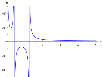
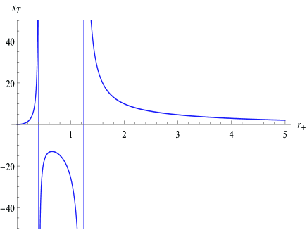
Figure 4: (a) $\alpha$ vs. $r_{+}$ for $k=1,n=6,\alpha=1,\Phi=1,\Lambda=-2$ (b) $\kappa_{T}$ vs. $r_{+}$ for $k=1,n=6,\alpha=1,\Phi=1,\Lambda=-2$

From the definitions of $\alpha$ and $C_{\Phi}$, one can obtain

$$Q\alpha=(\frac{\partial Q}{\partial T})_{\Phi}=(\frac{\partial Q}{\partial S})_{\Phi}(\frac{\partial S}{\partial T})_{\Phi}=(\frac{\partial Q}{\partial S})_{\Phi}(\frac{C_{\Phi}}{T}).$$ (34)

So the R.H.S of Eq.(30) can be derived as

$$\frac{\Delta C_{\Phi}}{TQ\Delta\alpha}=(\frac{\partial S}{\partial Q})_{\Phi}=\frac{(n-1)\pi(r_{+}^{2}+k\alpha)^{2}}{(n-2)^{2}r_{+}^{3}\Phi}.$$ (35)

On the other hand, the L.H.S of Eq.(30) can be derived as

$$-(\frac{\partial\Phi}{\partial T})_{S}=\frac{(n-1)\pi(r_{+}^{2}+k\alpha)^{2}}{(n-2)^{2}r_{+}^{3}\Phi}.$$ (36)

So the first equation of Erhenfest equations has been proved to be valid.

The L.H.S of Eq.(31) can be obtained as

$$-\left(\frac{\partial\Phi}{\partial T}\right)_{Q}=\frac{-1}{\left(\frac{\partial T}{\partial\Phi}\right)_{Q}}=\frac{-1}{\left(\frac{\partial T}{\partial\Phi}\right)_{r_{+}}+\left(\frac{\partial T}{\partial r_{+}}\right)_{\Phi}\left(\frac{\partial r_{+}}{\partial\Phi}\right)_{Q}}=\frac{-1}{\left(\frac{\partial T}{\partial\Phi}\right)_{r_{+}}}=\frac{(n-1)\pi(r_{+}^{2}+k\alpha)^{2}}{(n-2)^{2}r_{+}^{3}\Phi}.$$ (37)

Note that we have utilized the phase transition condition $\left(\frac{\partial T}{\partial r_{+}}\right)_{\Phi}=0$. From the thermodynamic identity Banerjee5

$$(\frac{\partial Q}{\partial\Phi})_{T}(\frac{\partial\Phi}{\partial T})_{Q}(\frac{\partial T}{\partial Q})_{\Phi}=-1,$$ (38)

we can derive that

$$Q\kappa_{T}=(\frac{\partial Q}{\partial\Phi})_{T}=-(\frac{\partial T}{\partial\Phi})_{Q}(\frac{\partial Q}{\partial T})_{\Phi}=-(\frac{\partial T}{\partial\Phi})_{Q}Q\alpha.$$ (39)

Noting that in the above derivation, we have also utilized both the definitions of $\kappa_{T}$ and $\alpha$. We can obtain

$$\frac{\Delta\alpha}{\Delta\kappa_{T}}=-(\frac{\partial\Phi}{\partial T})_{Q}=\frac{(n-1)\pi(r_{+}^{2}+k\alpha)^{2}}{(n-2)^{2}r_{+}^{3}\Phi}.$$ (40)

From Eqs.(37) and (40), one can easily draw the conclusion that the second equation of Ehrenfest equations also holds. The Prigogine-Defay(PD) ratio can be calculated as

$$\Pi=\frac{\Delta C_{\Phi}\Delta\kappa_{T}}{T_{c}Q(\Delta\alpha)^{2}}=1.$$ (41)

Eq.(41) and the validity of Ehrenfest equations show that Lovelock AdS black holes in grand canonical ensemble undergo second order phase transition.

IV Thermodynamic geometry of Lovelock AdS black holes

Weinhold’s metric Weinhold and Ruppeiner’s metric Ruppeiner are defined respectively as

$$g_{ij}^{W} = \frac{\partial^{2}U(x^{k})}{\partial x^{i}\partial x^{j}},$$ (42)

$$g_{ij}^{R} = -\frac{\partial^{2}S(x^{k})}{\partial x^{i}\partial x^{j}}.$$ (43)

And they are conformally connected to each other through the map Janyszek

$$dS^{2}_{R}=\frac{dS^{2}_{W}}{T}.$$ (44)

Utilizing Eqs.(19) and (21), one can obtain the components of Weinhold’s metric as

$$g_{SS}^{W} = \frac{D(r_{+},Q)}{3(n-1)^{2}\pi r_{+}^{3n-4}(r_{+}^{2}+k\alpha)^{5}\Sigma_{k}^{3}},$$ (45)

$$g_{QQ}^{W} = \frac{4\pi}{(n-2)r_{+}^{n-2}\Sigma_{k}},$$ (46)

$$g_{SQ}^{W} = g_{QS}^{W}=\frac{-16\pi Q}{(n-1)r_{+}^{2n-7}(r_{+}^{2}+k\alpha)^{2}\Sigma_{k}^{2}},$$ (47)

where

$$D(r_{+},Q) = 96\pi^{2}Q^{2}r_{+}^{8}\left[(2n-3)r_{+}^{2}+k(2n-7)\alpha\right]-r_{+}^{2n}$$ (48)

$$\times\left\{k(n-1)\left[3(n-2)r_{+}^{6}-18kr_{+}^{4}\alpha+2k^{2}(n-9)r_{+}^{2}\alpha^{2}+k^{3}(n-6)\alpha^{3}\right]+6r_{+}^{6}\Lambda(r_{+}^{2}+5k\alpha)\right\}\Sigma_{k}^{2}.$$

Utilizing Eqs.(17), (44), (45), (46) and (47), the components of Ruppeiner’s metric can be derived as

$$g_{11}^{R} = \frac{4r_{+}^{5-3n}D(r_{+},Q)}{(n-1)(r_{+}^{2}+k\alpha)^{3}\left\{k(n-1)\left[3(n-2)r_{+}^{4}+3k(n-4)r_{+}^{2}\alpha+k^{2}(n-6)\alpha^{2}\right]\Sigma_{k}^{3}-6r_{+}^{6}\Lambda\Sigma_{k}^{3}-96\pi^{2}Q^{2}r_{+}^{8-2n}\Sigma_{k}\right\}},$$

(49)

$$g_{22}^{R} = \frac{48(n-1)\pi^{2}r_{+}^{n+3}(r_{+}^{2}+k\alpha)^{2}\Sigma_{k}}{(n-2)\left\{-96\pi^{2}Q^{2}r_{+}^{8}+r_{+}^{2n}(n-1)k\left[3(n-2)r_{+}^{4}+3k(n-4)r_{+}^{2}\alpha+k^{2}(n-6)\alpha^{2}\right]\Sigma_{k}^{2}-6r_{+}^{2n+6}\Lambda\Sigma_{k}^{2}\right\}},$$ (50)

$$g_{12}^{R} = g_{21}^{R}=\frac{-192\pi^{2}Qr_{+}^{8-2n}}{k(n-1)\left[3(n-2)r_{+}^{4}+3k(n-4)r_{+}^{2}\alpha+k^{2}(n-6)\alpha^{2}\right]\Sigma_{k}^{2}-6r_{+}^{6}\Lambda\Sigma_{k}^{2}-96\pi^{2}Q^{2}r_{+}^{8-2n}}.$$ (51)

Utilizing Eqs.(49)-(51), we can obtain Ruppeiner scalar curvature as

$$R=\frac{E(r_{+},\Phi)}{F(r_{+},\Phi)},$$ (52)

where

$$F(r_{+},\Phi) = -(n-1)r_{+}^{n}(r_{+}^{2}+k\alpha)^{3}\Sigma_{k}\times\{-6\Lambda r_{+}^{8}-3r_{+}^{6}\left[k(2+n^{2}-3n+10\alpha\Lambda)-2(n-2)^{2}\Phi^{2}\right]$$ (53)

$$+18k\alpha r_{+}^{4}\left[k(n-1)-(n-2)^{2}\Phi^{2}\right]-2k^{3}(n-9)(n-1)\alpha^{2}r_{+}^{2}-k^{4}(n-6)(n-1)\alpha^{3}\}^{3}$$

$$\times\left[3k(n-2)(n-1)r_{+}^{4}+3k^{2}(n-4)(n-1)r_{+}^{2}\alpha+k^{3}(n-6)(n-1)\alpha^{2}-6r_{+}^{6}\Lambda-6(n-2)^{2}r_{+}^{4}\Phi^{2}\right],$$

and $E(r_{+},Q)$ is too lengthy to be displayed here. The above result has been rewritten in the function of $\Phi$ so that we can compare it with the specific heat. It is not difficult to observe from Eq.(52) that in the denominator of Ruppeiner scalar curvature, the fifth factor is exactly one quarter of the denominator of the specific heat while the last factor coincides with the numerator of the Hawking temperature. In other words, the Ruppeiner scalar curvature may diverge exactly where the specific heat diverges. It also reveals the extremal black hole condition that the Hawking temperature is zero. For an intuitive understanding, one can observe the behavior of Ruppeiner scalar curvature $R$ in Fig.5. Comparing Fig.5 with Fig.1, one can find that the divergence structures of both the Ruppeiner scalar curvature and the specific heat are exactly the same. And the Ruppeiner metric does provide a wonderful tool for one to probe the phase structures of black holes.

Among thermodynamic geometry theories, Ruppeiner geometry has been proved to be outstanding for its profound physical meaning. As argued in Ref. Ruppeiner2 , Ruppeiner scalar curvature $R$ results from the thermodynamic information metric giving thermodynamic fluctuations and may be interpreted physically as the measurement of the correlation between fluctuating Planck length pixels of event horizon. In the region with positive $R$, repulsive interactions (Fermionic behavior) dominate while in the region with negative $R$, attractive interactions (Bosonic behavior) dominate. Moreover, $\mid R\mid$ indicates the average size of fluctuations.

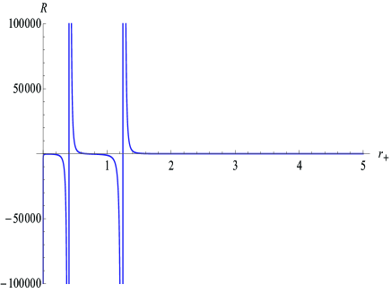
Figure 5: Ruppeiner scalar curvature $R$ vs. $r_{+}$ for $k=1,n=6,\alpha=1,\Phi=1,\Lambda=-2$

V Concluding Remarks

In this paper, we extend our former research of charged topological Lovelock AdS black holes to the non-extended phase space. Specifically, we investigate phase transition of (n+1)-dimensional Lovelock AdS black holes in the grand canonical ensemble. Firstly, we calculated the specific heat at constant electric potential. To probe the impact of the various parameters, we utilize the control variate method and solve the phase transition condition equation numerically for the case $k=1,-1$. There are two critical points for the case $n=6,k=1$ while there is only one for other cases. And the distance between the two phase transition points becomes larger with the increasing of $\Lambda$ and $\Phi$ while it first becomes larger then becomes smaller with the increasing of $\alpha$. We also study the behavior of specific heat graphically. As can be seen from the graph, the black holes can be divided into three phases. Namely, small stable ($C_{\Phi}>0$) black hole, medium unstable ($C_{\Phi}<0$) black hole and large stable ($C_{\Phi}>0$) black hole. The graph of Hawking temperature is also depicted to check whether the phase transition points locate in the physical region. For $k=0$, there exists no phase transition point.

To figure out the nature of phase transition in the grand canonical ensemble, we carry out an analytic check of the analog form of Ehrenfest equations proposed by Banerjee et al. It is proved that the two Ehrenfest equations hold at the phase transition point. Prigogine-Defay ratio is also calculated. Based on these results, one can draw the conclusion that Lovelock AdS black holes in grand canonical ensemble undergo a second order phase transition.

To examine the phase structure in the grand canonical ensemble, we also utilize the thermodynamic geometry method. Specifically, we calculate both the Weinhold metric and Ruppeiner metric. It is shown that in the denominator of Ruppeiner scalar curvature, the fifth factor is exactly one quarter of the denominator of the specific heat while the last factor coincides with the numerator of the Hawking temperature. So the Ruppeiner scalar curvature may diverge exactly where the specific heat diverges. It also reveals the extremal black hole condition that the Hawking temperature is zero. From the graph of Ruppeiner scalar curvature, one can see clearly that the divergence structures of both the Ruppeiner scalar curvature and the specific heat are exactly the same. Our research provides one more example that Ruppeiner metric serves as a wonderful tool to probe the phase structures of black holes.

Note that one may vary the spatial dimension, the cosmological constant, and the coefficients of the curvature terms in the Lagrangian and we mainly concentrate on a few instances of a very large model in this paper. The control variate method has been utilized to crack down the problem of probing the impact of the various parameters. We choose such parameter regions that we can compare our results with those in former literatures. One can easily extend our results to more cases. The black hole solution here was derived for the special case that the second and third order Lovelock coefficients satisfy certain conditions. Phase transition in the non-extended space of more general black hole solutions in Lovelock gravtiy would be further investigated in our future work. Also note that the methods utilized in this paper can be generalized to an arbitrary non-linear electrodynamics Lagrangian, the specific results in this paper however are model-dependent. For a more general analysis, we would like to draw the readers’ attention to the excellent work Miskovic99 , where the authors presented an elegant procedure for Gauss-Bonnet gravity regardless of the explicit form of the nonlinear electrodynamics Lagrangian. It certainly deserves to extend this treatment to the third-order Lovelock case in future research.

References

- (1) J. X. Mo and W. B. Liu, P-V criticality of topological black holes in Lovelock-Born-Infeld gravity, Eur. Phys. J. C 74 (2014)2836.
- (2) A. Belhaj, M. Chabab, H. EL Moumni, K. Masmar and M. B. Sedra, Ehrenfest Scheme of Higher Dimensional Topological AdS Black Holes in Lovelock-Born-Infeld Gravity, arXiv:1405.3306.
- (3) H. Xu, W. Xu and L. Zhao, Extended phase space thermodynamics for third order Lovelock black holes in diverse dimensions, arXiv:1405.4143.
- (4) A. M. Frassino, D. Kubiznak, R. B. Mann, F. Simovic, Multiple Reentrant Phase Transitions and Triple Points in Lovelock Thermodynamics, arXiv:1406.7015.
- (5) B. P. Dolan, A. Kostouki, D. Kubiznak and R. B. Mann, Isolated critical point from Lovelock gravity, arXiv:1407.4783.
- (6) D. Lovelock, The Einstein tensor and its generalizations, J. Math. Phys. (N.Y.) 12 (1971)498.
- (7) D. G. Boulware and S. Deser, String-Generated Gravity Models, Phys. Rev. Lett. 55 (1985)2656.
- (8) M. H. Dehghani, N. Alinejadi and S. H. Hendi, Topological Black Holes in Lovelock-Born-Infeld Gravity, Phys. Rev. D 77 (2008)104025 [arXiv:0802.2637].
- (9) M. H. Dehghani and M. Shamirzaie, Thermodynamics of asymptotic flat charged black holes in third order Lovelock gravity, Phys. Rev. D 72 (2005)124015 [arXiv:hep-th/0506227].
- (10) M. H. Dehghani and R. B. Mann, Thermodynamics of rotating charged black branes in third order Lovelock gravity and the counterterm method, Phys. Rev. D 73 (2006)104003 [arXiv:hep-th/0602243].
- (11) M. H. Dehghani and N. Farhangkhah, Asymptotically Flat Radiating Solutions in Third Order Lovelock Gravity, Phys. Rev. D 78 (2008) 064015 [arXiv:0806.1426].
- (12) M. H. Dehghani and R. Pourhasan, Thermodynamic instability of black holes of third order Lovelock gravity, Phys. Rev. D 79 (2009)064015 [arXiv:0903.4260].
- (13) M. H. Dehghani and R. B. Mann, Lovelock-Lifshitz Black Holes, JHEP 1007 (2010) 019 [arXiv:1004.4397].
- (14) M. H. Dehghani and Sh. Asnafi, Thermodynamics of Rotating Lovelock-Lifshitz Black Branes, Phys. Rev. D 84 (2011) 064038 [arXiv:1107.3354].
- (15) M. Aiello, R. Ferraro and G. Giribet, Exact solutions of Lovelock-Born-Infeld black holes, Phys. Rev. D 70 (2004) 104014 [arXiv:gr-qc/0408078].
- (16) G. Kofinas and R. Olea, Universal regularization prescription for Lovelock AdS gravity, JHEP 0711 (2007) 069 [arXiv:0708.0782].
- (17) R. Banerjee and S. K. Modak, Quantum Tunneling, Blackbody Spectrum and Non-Logarithmic Entropy Correction for Lovelock Black Holes, JHEP 0911 (2009)073 [arXiv:0908.2346].
- (18) H. Maeda, M. Hassaine and C. Martinez, Lovelock black holes with a nonlinear Maxwell field, Phys. Rev. D 79 (2009) 044012 [arXiv:0812.2038].
- (19) J. de Boer, M. Kulaxizi and A. Parnachev, Holographic Lovelock Gravities and Black Holes, JHEP 1006 (2010)008 [arXiv:0912.1877].
- (20) R. G. Cai, L. M. Cao and N. Ohta, Black Holes without Mass and Entropy in Lovelock Gravity, Phys. Rev. D 81 (2010) 024018 [arXiv:0911.0245].
- (21) D. Kastor, S. Ray, J. Traschen, Smarr Formula and an Extended First Law for Lovelock Gravity, Class. Quant. Grav. 27 (2010) 235014 [arXiv:1005.5053].
- (22) S. H. Mazharimousavi and M. Halilsoy Solution for Static, Spherically Symmetric Lovelock Gravity Coupled with Yang-Mills hierarchy, Phys. Lett. B 694 (2010) 54-60 [arXiv:1007.4888].
- (23) D. Zou, R. Yue and Z. Yang, Thermodynamics of third order Lovelock anti-de Sitter black holes revisited, Commun. Theor. Phys. 55 (2011) 449-456 [arXiv:1011.2595].
- (24) P. Li, R. H. Yue and D. C. Zou, Thermodynamics of Third Order Lovelock-Born-Infeld Black Holes, Commun. Theor. Phys. 56 (2011)845-850 [arXiv:1110.0064].
- (25) S. Sarkar and A. C. Wall, Second Law Violations in Lovelock Gravity for Black Hole Mergers, Phys. Rev. D 83 (2011) 124048 [arXiv:1011.4988].
- (26) J. de Boer, M. Kulaxizi and A. Parnachev, Holographic Entanglement Entropy in Lovelock Gravities, JHEP 1107 (2011) 109 [arXiv:1101.5781].
- (27) Y. Bardoux, C. Charmousis and T. Kolyvaris, Lovelock solutions in the presence of matter sources, Phys. Rev. D 83 (2011) 104020 [arXiv:1012.4390].
- (28) S. H. Hendi, S. Panahiyan and H. Mohammadpour, Third order Lovelock black branes in the presence of a nonlinear electromagnetic field, Eur. Phys. J. C 72 (2012)2184.
- (29) R. Yue, D. Zou, T. Yu, P. Li and Z. Yang, Slowly rotating charged black holes in anti-de Sitter third order Lovelock gravity, Gen. Rel. Grav. 43 (2011) 2103-2114 [arXiv:1011.5293].
- (30) M. Cruz, E. Rojas, Born-Infeld extension of Lovelock brane gravity, Class. Quant. Grav. 30 (2013) 115012 [arXiv:1212.1704].
- (31) T. Padmanabhan and D. Kothawala, Lanczos-Lovelock models of gravity, Phys. Rept. 531 (2013)115-171 [arXiv:1302.2151].
- (32) D. C. Zou, S. J. Zhang and B. Wang, The holographic charged fluid dual to third order Lovelock gravity, Phys. Rev. D 87 (2013)084032 [arXiv:1302.0904].
- (33) B. Chen, J. J. Zhang, Note on generalized gravitational entropy in Lovelock gravity, JHEP 07 (2013)185 [arXiv:1305.6767].
- (34) M. B. Gaete and M. Hassaine, Planar AdS black holes in Lovelock gravity with a nonminimal scalar field, JHEP 1311 (2013) 177 [arXiv:1309.3338].
- (35) A. Lala, Critical phenomena in higher curvature charged AdS black holes Adv.High Energy Phys. 2013 (2013) 918490
- (36) Z. Amirabi, Black hole solution in third order Lovelock gravity has no Gauss-Bonnet limit, Phys. Rev. D 88 (2013)087503 [arXiv:1311.4911].
- (37) R. Banerjee, S. K. Modak and S. Samanta, Glassy Phase Transition and Stability in Black Holes, Eur. Phys. J. C 70 (2010) 317 [arXiv:1002.0466].
- (38) R. Banerjee, S. K. Modak and S. Samanta, Second Order Phase Transition and Thermodynamic Geometry in Kerr-AdS Black Hole, Phys. Rev. D 84 (2011) 064024 [arXiv:1005.4832].
- (39) R. Banerjee and D. Roychowdhury, Critical phenomena in Born-Infeld AdS black holes, Phys. Rev. D 85 (2011) 044040 [arXiv:1111.0147].
- (40) R. Banerjee, S. Ghosh and D. Roychowdhury, New type of phase transition in Reissner Nordstrom - AdS black hole and its thermodynamic geometry, Phys. Lett. B 696, 156 (2011) 156 [arXiv:1008.2644].
- (41) R. Banerjee and D. Roychowdhury, Thermodynamics of phase transition in higher dimensional AdS black holes, JHEP 11 (2011) 004 [arXiv:1109.2433].
- (42) R. Banerjee, S. K. Modak and D. Roychowdhury, A unified picture of phase transition: from liquid-vapour systems to AdS black holes , JHEP 1210 (2012) 125 [arXiv:1106.3877].
- (43) J. X. Mo, X. X. Zeng, G. Q. Li, X. Jiang, W. B. Liu, A unified phase transition picture of the charged topological black hole in Hořava-Lifshitz gravity, JHEP 1310 (2013)056.
- (44) J. X. Mo and W. B. Liu, Ehrenfest scheme for P-V criticality in the extended phase space of black holes, Phys. Lett. B 727 (2013) 336-339.
- (45) J. X. Mo and W. B. Liu, Ehrenfest scheme for - criticality of higher dimensional charged black holes, rotating black holes and Gauss-Bonnet AdS black holes, Phys. Rev. D 89 (2014) 084057.
- (46) Z. Zhao and J. Jing, Ehrenfest scheme for complex thermodynamic systems in full phase space, arXiv:1405.2640.
- (47) F. Weinhold, Metric geometry of equilibrium thermodynamics, Chem.Phys. 63 (1975) 2479.
- (48) G. Ruppeiner, A Riemannian geometric model, Phys. Rev. A 20 (1979) 1608.
- (49) H. Quevedo, Geometrothermodynamics, J. Math. Phys. 48 (2007) 013506 [arXiv:physics/0604164].
- (50) G. Ruppeiner, Thermodynamic curvature and black holes, arXiv:1309.0901.
- (51) R. Tharanath, J. Suresh, N. Varghese and V. C. Kuriakose, Thermodynamic Geometry of Reissener-Nordström-de Sitter black hole and its extremal case, arXiv:1404.6789.
- (52) J. Suresh, R. Tharanath, N. Varghese and V. C. Kuriakose, The thermodynamics and thermodynamic geometry of the Park black hole, Eur. Phys. J. C 74 (2014) 2819.
- (53) S. A. H. Mansoori, B. Mirza, Correspondence of phase transition points and singularities of thermodynamic geometry of black holes, Eur. Phys. J. C 74 (2014) 2681.
- (54) M. B. J. Poshteh, B. Mirza, Z. Sherkatghanad, Phase transition, critical behavior, and critical exponents of Myers-Perry black holes, Phys. Rev. D 88 (2013) 024005
- (55) S. W. Wei and Y. X. Liu, Critical phenomena and thermodynamic geometry of charged Gauss-Bonnet AdS black holes Phys. Rev. D 87 (2013) 044014
- (56) S. W. Wei and Y. X. Liu, Thermodynamic Geometry of black hole in the deformed Horava-Lifshitz gravity, Europhys.Lett. 99 (2012) 20004
- (57) A. Lala and D. Roychowdhury, Ehrenfest’s scheme and thermodynamic geometry in Born-Infeld AdS black holes, Phys. Rev. D 86 (2012) 084027
- (58) G. Ruppeiner, Thermodynamic curvature: pure fluids to black holes, J. Phys.: Conf. Series 410 (2013) 012138 [arXiv:1210.2011]
- (59) S. Bellucci and B. N. Tiwari , Thermodynamic Geometry and Topological Einstein-Yang-Mills Black Holes, Entropy 14 (2012) 1045
- (60) A. Lala and D. Roychowdhury, Ehrenfest’s scheme and thermodynamic geometry in Born-Infeld AdS black holes, Phys. Rev. D 86 (2012) 084027
- (61) Y. D. Tsai, X. N. Wu and Y. Yang, Phase Structure of Kerr-AdS Black Hole, Phys. Rev. D 85 (2012) 044005
- (62) C. Niu, Y. Tian, X. N. Wu, Critical Phenomena and Thermodynamic Geometry of RN-AdS Black Holes, Phys. Rev. D 85 (2012) 024017
- (63) H. Janyszek and R. Mrugala, Geometrical structure of the state space in classical statistical and phenomenological thermodynamics, Rep.Math.Phys. 27 (1989) 145
- (64) O. Miskovic and R. Olea, Quantum statistical relation for black holes in nonlinear electrodynamics coupled to Einstein-Gauss-Bonnet AdS gravity, Phys. Rev. D 83 (2011) 064017