Abstract

We consider discretizations of the hyper-singular integral operator on closed surfaces and show that the inverses of the corresponding system matrices can be approximated by blockwise low-rank matrices at an exponential rate in the block rank. We cover in particular the data-space format of $\mathcal{H}$-matrices. We show the approximability result for two types of discretizations. The first one is a saddle point formulation, which incorporates the constraint of vanishing mean of the solution. The second discretization is based on a stabilized hyper-singular operator, which leads to symmetric positive definite matrices. In this latter setting, we also show that the hierarchical Cholesky factorization can be approximated at an exponential rate in the block rank.

1 Introduction

Boundary element method (BEM) are obtained as the discretizations of boundary boundary integral equations. These arise, for example, when elliptic partial differential equations are reformulated as integral equations on the boundary $\Gamma:=\partial\Omega$ of a domain $\Omega\subset\mathbb{R}^{d}$. A particular strength of these methods is that they can deal with unbounded exterior domains. Reformulating an equation posed in a volume as one on its boundary brings about a significant reduction in complexity. However, the boundary integral operators are fully occupied, and this has sparked the development of various matrix compression techniques. One possibility, which we will not pursue here, are wavelet compression techniques, [Rat98, Rat01, Sch98a, vPSS97, Tau03, TW03], where sparsity of the system matrices results from the choice of basis. In the present work, we will consider data-sparse matrix formats that are based on blockwise low-rank matrices. These formats can be traced back to multipole expansions, [Rok85, GR97], panel clustering, [NH88, HN89, HS93, Sau92], and were then further developed in the mosaic-skeleton method, [Tyr00], the adaptive cross approximation (ACA) method, [Beb00], and the hybrid cross approximation (HCA), [BG05]. A fairly general framework for these techniques is given by the ${\mathcal{H}}$-matrices, introduced in [Hac99, GH03, Gra01, Hac09] and the $\mathcal{H}^{2}$-matrices, [HKS00, Bör10a, Bör10b]. Both $\mathcal{H}$- and $\mathcal{H}^{2}$-matrices come with an (approximate) arithmetic and thus provide the possibility of (approximately) inverting or factorizing a BEM matrix; also algebraic approaches to the design of preconditioners for boundary element discretizations, both for positive and negative order operators, are available with this framework. Empirically, it has already been observed in [Gra01, Beb05b] that such an approach works well in practice.

Mathematically, the fundamental question in connection with the $\mathcal{H}$-matrix arithmetic is whether the desired result, i.e., the inverse (or a factorization such as an $LU$- or Cholesky factorization), can be represented accurately in near optimal complexity in this format. This question is answered in the affirmative in the present work for discretizations of the hyper-singular integral operator associated with the Laplace operator. In previous work, we showed similar existence results for FEM discretizations [FMP13b] and the discretization of the single layer operator, [FMP13a]. Compared to the symmetric positive definite case of the single layer operator studied in [FMP13a], the hyper-singular operator on closed surfaces has a one-dimensional kernel and is naturally treated as a (simple) saddle point problem. We show in Theorem 2.6 (cf. also Remark 2.7) that the inverse of the discretization of this saddle point formulation can be approximated by blockwise low-rank matrices at an exponential rate in the block rank. A corresponding approximation result for the discretized version of the stabilized hyper-singular operator follows then fairly easily in Corollary 5.1. The approximation result Theorem 2.6 also underlies our proof that the hierarchical Cholesky factorization of the stabilized hyper-singular operator admits an efficient representation in the $\mathcal{H}$-matrix format (Theorem 6.1).

The approximability problem for the inverses of Galerkin BEM-matrices has previously only been studied in [FMP13a] for the single layer operator. In a FEM context, works prior to [FMP13b] include [BH03, Beb05a, Beb05b], [Sch06], and [Bör10a]. These works differ from [FMP13b, FMP13a] and the present paper in an important technical aspect: while [FMP13b, FMP13a] and the present analysis analyze the discretized operators and show exponential convergence in the block rank, the above mentioned works study first low-rank approximations on the continuous level and transfer these to the discrete level in a final projection step. Therefore, they achieve exponential convergence in the block rank up to this projection error, which is related to the discretization error.

The paper is structured as follows. In the interest of readability, we have collected the main result concerning the approximability of the inverse of the discretization of the saddle point formulation in Section 2. The mathematical core is found in Section 3, where we study how well solutions of the (discretized) hyper-singular integral equation can be approximated from low-dimensional spaces (Theorem 3.1). In contrast to [FMP13a], which considered only lowest-order discretization, we consider here arbitrary fixed-order discretizations. The approximation result of Section 3 can be translated to the matrix level, which is done in Section 4. Section 5 shows how the results for the saddle point formulation imply corresponding ones for the stabilized hyper-singular operator. Finally, Section 6 provides the existence of an approximate $\mathcal{H}$-Cholesky decomposition. We close with numerical examples in Section 7.

We use standard integer order Sobolev spaces and the fractional order Sobolev spaces $H^{1/2}(\Gamma)$ and its dual $H^{-1/2}(\Gamma)$ as defined in, e.g., [SS11]. The notation $\lesssim$ abbreviates $\leq$ up to a constant $C>0$ that depends only on the domain $\Omega$, the spatial dimension $d$, the polynomial degree $p$, and the $\gamma$-shape regularity of $\mathcal{T}_{h}$. It does not, however, depend on critical parameters such as the mesh size $h$, the dimension of the finite dimensional BEM space, or the block rank employed. Moreover, we use $\simeq$ to indicate that both estimates $\lesssim$ and $\gtrsim$ hold.

2 Main Result

2.1 Notation and setting

Throughout this paper, we assume that $\Omega\subset\mathbb{R}^{d}$, $d\in\{2,3\}$ is a bounded Lipschitz domain such that $\Gamma:=\partial\Omega$ is polygonal (for $d=2$) or polyhedral (for $d=3$). We assume that $\Gamma$ is connected.

We consider the hyper-singular integral operator $W\in L(H^{1/2}(\Gamma),H^{-1/2}(\Gamma))$ given by

$$Wv(x)=-\gamma_{1,x}^{\text{int}}(\widetilde{K}v)(x)=-\gamma_{1,x}^{\text{int}}\int_{\Gamma}(\gamma_{1,y}^{\text{int}}G(x-y))v(y)ds_{y},\quad x\in\Gamma,$$

where $G(x)=-\frac{1}{2\pi}\log\left|x\right|$ for $d=2$ and $G(x)=\frac{1}{4\pi}\frac{1}{\left|x\right|}$ for $d=3$ is the fundamental solution associated with the Laplacian. Here, the double layer potential $\widetilde{K}\in L(H^{1/2}(\Gamma),H^{1}(\Omega))$ is given by $\widetilde{K}v(x):=\int_{\Gamma}(\gamma_{1,y}^{\text{int}}G(x-y))v(y)ds_{y}$, where $\gamma_{1,z}^{\text{int}}$ denotes the interior conormal derivative at the point $z\in\Gamma$, i.e., with the normal vector $n(z)$ at $z\in\Gamma$ pointing into $\Omega^{c}$ and some sufficiently smooth function $u$ defined in $\Omega$ one requires $\gamma_{1,z}^{\text{in}}u=\nabla u(z)\cdot n(z)$.

The hyper-singular integral operator $W$ is symmetric, positive semidefinite on $H^{1/2}(\Gamma)$. Since $\Gamma$ is connected, $W$ has a one-dimensional kernel given by the constant functions. In order to deal with this kernel, we can either use factor spaces, stabilize the operator, or study a saddle point formulation. In the following, we will employ the latter by adding the side constraint of vanishing mean. In Section 5 we will very briefly study the case of the stabilized operator, and our analysis of Cholesky factorizations in Section 6 will be performed for the stabilized operator.

With the bilinear form $b(v,\mu):=\mu\int_{\Gamma}vds_{x}$, we get the saddle point formulation of the boundary integral equation

$$W\phi=f\quad\text{on}\;\Gamma$$

with arbitrary $f\in H^{-1/2}(\Gamma)$ as finding $(\phi,\lambda)\in H^{1/2}(\Gamma)\times\mathbb{R}$ such that

$$\left<W\phi,\psi\right>+b(\psi,\lambda) =\left<f,\psi\right>\qquad\forall\psi\in H^{1/2}(\Gamma),$$ (2.1a)

$$b(\phi,\mu) =0\qquad\forall\mu\in\mathbb{R}.$$ (2.1b)

By classical saddle-point theory, this problem has a unique solution $(\phi,\lambda)\in H^{1/2}(\Gamma)\times\mathbb{R}$, since the bilinear form $b$ satisfies an inf-sup condition, and the bilinear form $\left<W\phi,\psi\right>$ is coercive on the kernel of $b(\cdot,\lambda)$, which is just the one-dimensional space of constant functions (see, e.g., [SS11]).

For the discretization, we assume that $\Gamma$ is triangulated by a (globally) quasiuniform mesh ${\mathcal{T}}_{h}=\{T_{1},\dots,T_{M}\}$ of mesh width $h:=\max_{T_{j}\in\mathcal{T}_{h}}{\rm diam}(T_{j})$. The elements $T_{j}\in\mathcal{T}_{h}$ are open line segments ($d=2$) or triangles ($d=3$). Additionally, we assume that the mesh $\mathcal{T}_{h}$ is regular in the sense of Ciarlet and $\gamma$-shape regular in the sense that for $d=2$ the quotient of the diameters of neighboring elements is bounded by $\gamma$ and for $d=3$ we have ${\rm diam}(T_{j})\leq\gamma\,|T_{j}|^{1/2}$ for all $T_{j}\in\mathcal{T}_{h}$, where $|T_{j}|=\operatorname*{area}(T_{j})$ denotes the length/area of the element $T_{j}$.

We consider the Galerkin discretization of $W$ by continuous, piecewise polynomial functions of fixed degree $p\geq 1$ in $S^{p,1}({\mathcal{T}}_{h}):=\{u\in C(\Gamma)\,:\,u|_{T}\in P_{p}(T)\,\forall T\in\mathcal{T}_{h}\}$, where $P_{p}(T)$ denotes the space of polynomials of maximal degree $p$ on the triangle $T$. We choose a basis of $S^{p,1}({\mathcal{T}}_{h})$, which is denoted by ${\mathcal{B}}_{h}:=\{\psi_{j}\,:\,j=1,\dots,N\}$. Given that our results are formulated for matrices, assumptions on the basis ${\mathcal{B}}_{h}$ need to be imposed. For the isomorphism $\Phi:\mathbb{R}^{N}\rightarrow S^{p,1}({\mathcal{T}}_{h})$, $\mathbf{x}\mapsto\sum_{j=1}^{N}x_{j}\psi_{j}$, we require

$$h^{(d-1)/2}\left\|\mathbf{x}\right\|_{2}\lesssim\left\|\Phi(\mathbf{x})\right\|_{L^{2}(\Gamma)}\lesssim h^{(d-1)/2}\left\|\mathbf{x}\right\|_{2}\quad\forall\,\mathbf{x}\in\mathbb{R}^{N}.$$ (2.2)

Remark 2.1

The standard basis for $p=1$ consists of the classical hat functions satisfying $\psi_{j}(x_{i})=\delta_{ij}$ and for $p\geq 2$ we refer to, e.g., [Sch98b, KS99, DKP⁺08]. These bases satisfy assumption (2.2).  

The discrete variational problem is given by finding $(\phi_{h},\lambda_{h})\in S^{p,1}(\mathcal{T}_{h})\times\mathbb{R}$ such that

$$\left<W\phi_{h},\psi_{h}\right>+b(\psi_{h},\lambda_{h}) = \left<f,\psi_{h}\right>\qquad\forall\psi_{h}\in S^{p,1}(\mathcal{T}_{h}),$$ (2.3)

$$b(\phi_{h},\mu) = 0\qquad\forall\mu\in\mathbb{R}.$$

Since the bilinear form $b$ trivially satisfies a discrete inf-sup condition, the discrete problem is uniquely solvable as well, and one has the stability bounds

$$\left\|\phi_{h}\right\|_{H^{1/2}(\Gamma)}+|\lambda|\leq C\left\|f\right\|_{H^{-1/2}(\Gamma)},$$ (2.4)

for a constant $C>0$ which depends only on $\Gamma$. For $f\in L^{2}(\Gamma)$ and the $L^{2}$-projection $\Pi^{L^{2}}:L^{2}(\Gamma)\rightarrow S^{p,1}(\mathcal{T}_{h})$, one even has the following estimate

$$\left\|\phi_{h}\right\|_{H^{1/2}(\Gamma)}+|\lambda|\leq C\left\|\Pi^{L^{2}}f\right\|_{L^{2}(\Gamma)}\leq C\left\|f\right\|_{L^{2}(\Gamma)}.$$ (2.5)

With the basis $\mathcal{B}_{h}$, the left-hand side of (2.3) leads to the invertible block matrix

$$\boldsymbol{\mathcal{W}}:=\begin{pmatrix}\mathbf{W}&\mathbf{B}\\ \mathbf{B}^{T}&0\end{pmatrix},$$ (2.6)

where the matrix $\mathbf{W}\in\mathbb{R}^{N\times N}$ and the vector $\mathbf{B}\in\mathbb{R}^{N\times 1}$ are given by

$$\mathbf{W}_{jk}=\left<W\psi_{k},\psi_{j}\right>,\quad\mathbf{B}_{j}=\left<\psi_{j},1\right>,\quad\psi_{k},\psi_{j}\in\mathcal{B}_{h}.$$ (2.7)

2.2 Approximation of $\boldsymbol{\mathcal{W}}^{-1}$ by blockwise low-rank matrices

Our goal is to approximate the inverse matrix $\boldsymbol{\mathcal{W}}^{-1}$ by $\mathcal{H}$-matrices, which are based on the concept that certain ’admissible’ blocks can be approximated by low-rank factorizations. The following definition specifies for which blocks such a factorization can be derived.

Definition 2.2 (bounding boxes and $\eta$-admissibility)

A cluster $\tau$ is a subset of the index set $\mathcal{I}=\{1,\ldots,N\}$. For a cluster $\tau\subset\mathcal{I}$, we say that $B_{R_{\tau}}\subset\mathbb{R}^{d}$ is a bounding box if:

1. $B_{R_{\tau}}$ is a hyper cube with side length $R_{\tau}$,

2. $\operatorname*{supp}\psi_{i}\subset B_{R_{\tau}}$ for all $i\in\tau$.

For an admissibility parameter $\eta>0$, a pair of clusters $(\tau,\sigma)$ with $\tau,\sigma\subset\mathcal{I}$ is $\eta$-admissible if there exist bounding boxes $B_{R_{\tau}}$, $B_{R_{\sigma}}$ satisfying (i)–(ii) such that

$$\min\{{\rm diam}(B_{R_{\tau}}),{\rm diam}(B_{R_{\sigma}})\}\leq\eta\;{\rm dist}(B_{R_{\tau}},B_{R_{\sigma}}).$$ (2.8)

Definition 2.3 (blockwise rank-$r$ matrices)

Let $P$ be a partition of ${\mathcal{I}}\times{\mathcal{I}}$ and $\eta>0$. A matrix ${\mathbf{W}}_{\mathcal{H}}\in\mathbb{R}^{N\times N}$ is said to be a blockwise rank-$r$ matrix, if for every $\eta$-admissible cluster pair $(\tau,\sigma)\in P$, the block ${\mathbf{W}}_{\mathcal{H}}|_{\tau\times\sigma}$ is a rank-$r$ matrix, i.e., it has the form ${\mathbf{W}}_{\mathcal{H}}|_{\tau\times\sigma}={\mathbf{X}}_{\tau\sigma}{\mathbf{Y}}^{T}_{\tau\sigma}$ with $\mathbf{X}_{\tau\sigma}\in\mathbb{R}^{\left|\tau\right|\times r}$ and $\mathbf{Y}_{\tau\sigma}\in\mathbb{R}^{\left|\sigma\right|\times r}$. Here and below, $\left|\sigma\right|$ denotes the cardinality of a finite set $\sigma$.

Definition 2.4 (cluster tree)

A cluster tree with leaf size $n_{\rm leaf}\in\mathbb{N}$ is a binary tree $\mathbb{T}_{\mathcal{I}}$ with root $\mathcal{I}$ such that for each cluster $\tau\in\mathbb{T}_{\mathcal{I}}$ the following dichotomy holds: either $\tau$ is a leaf of the tree and $\left|\tau\right|\leq n_{\rm leaf}$, or there exist sons $\tau^{\prime}$, $\tau^{\prime\prime}\in\mathbb{T}_{\mathcal{I}}$, which are disjoint subsets of $\tau$ with $\tau=\tau^{\prime}\cup\tau^{\prime\prime}$. The level function ${\rm level}:\mathbb{T}_{\mathcal{I}}\rightarrow\mathbb{N}_{0}$ is inductively defined by ${\rm level}(\mathcal{I})=0$ and ${\rm level}(\tau^{\prime}):={\rm level}(\tau)+1$ for $\tau^{\prime}$ a son of $\tau$. The depth of a cluster tree is ${\rm depth}(\mathbb{T}_{\mathcal{I}}):=\max_{\tau\in\mathbb{T}_{\mathcal{I}}}{\rm level}(\tau)$.

Definition 2.5 (far field, near field, and sparsity constant)

A partition $P$ of $\mathcal{I}\times\mathcal{I}$ is said to be based on the cluster tree $\mathbb{T}_{\mathcal{I}}$, if $P\subset\mathbb{T}_{\mathcal{I}}\times\mathbb{T}_{\mathcal{I}}$. For such a partition $P$ and a fixed admissibility parameter $\eta>0$, we define the far field and the near field as

$$P_{\rm far}:=\{(\tau,\sigma)\in P\;:\;(\tau,\sigma)\;\text{is $\eta$-admissible}\},\quad P_{\rm near}:=P\setminus P_{\rm far}.$$ (2.9)

The sparsity constant $C_{\rm sp}$ of such a partition was introduced in [Gra01] as

$$C_{\rm sp}:=\max\left\{\max_{\tau\in\mathbb{T}_{\mathcal{I}}}\left|\{\sigma\in\mathbb{T}_{\mathcal{I}}\,:\,\tau\times\sigma\in P_{\rm far}\}\right|,\max_{\sigma\in\mathbb{T}_{\mathcal{I}}}\left|\{\tau\in\mathbb{T}_{\mathcal{I}}\,:\,\tau\times\sigma\in P_{\rm far}\}\right|\right\}.$$ (2.10)

The following theorem is the main result of this paper. It states that the inverse matrix $\boldsymbol{\mathcal{W}}^{-1}$ can be approximated by an $\mathcal{H}$-matrix, where the approximation error in the spectral norm converges exponentially in the block rank.

Theorem 2.6

Fix an admissibility parameter $\eta>0$. Let a partition $P$ of $\mathcal{I}\times\mathcal{I}$ be based on the cluster tree $\mathbb{T}_{\mathcal{I}}$. Then, there exists a blockwise rank-$r$ matrix $\mathbf{V}_{\mathcal{H}}$ such that

$$\left\|\boldsymbol{\mathcal{W}}^{-1}|_{N\times N}-\mathbf{V}_{\mathcal{H}}\right\|_{2}\leq C_{\rm apx}C_{\rm sp}{\rm depth}(\mathbb{T}_{\mathcal{I}})N^{(2d-1)/(2d-2)}e^{-br^{1/(d+1)}}.$$

The constant $C_{\rm apx}$ depends only on $\Omega$, $d$, $p$, and the $\gamma$-shape regularity of the quasiuniform triangulation $\mathcal{T}_{h}$, while the constant $b>0$ additionally depends on $\eta$.

Remark 2.7 (approximation of inverse of full system)

The previous theorem provides an approximation $\mathbf{V}_{\mathcal{H}}$ to the first $N\times N$-subblock $\mathbf{V}$ of the matrix $\boldsymbol{\mathcal{W}}^{-1}=\begin{pmatrix}\mathbf{V}&\mathbf{P}\\ \mathbf{P}^{T}&0\end{pmatrix}$. Since $\mathbf{P}\in\mathbb{R}^{N\times 1}$ is a vector, the matrix $\widehat{\mathbf{V}}_{\mathcal{H}}=\begin{pmatrix}\mathbf{V}_{\mathcal{H}}&\mathbf{P}\\ \mathbf{P}^{T}&0\end{pmatrix}$ is a blockwise rank-$r$ approximation to the matrix $\boldsymbol{\mathcal{W}}^{-1}$ satisfying

$$\left\|\boldsymbol{\mathcal{W}}^{-1}-\widehat{\mathbf{V}}_{\mathcal{H}}\right\|_{2}\leq C_{\rm apx}C_{\rm sp}{\rm depth}(\mathbb{T}_{\mathcal{I}})N^{(2d-1)/(2d-2)}e^{-br^{1/(d+1)}}.$$

 

Remark 2.8 (relative errors)

In order to derive a bound for the relative error, we need an estimate on $\left\|\boldsymbol{\mathcal{W}}\right\|_{2}$, since $\frac{1}{\left\|{\boldsymbol{\mathcal{W}}}^{-1}\right\|_{2}}\leq\left\|\boldsymbol{\mathcal{W}}\right\|_{2}$. Since $\mathbf{W}$ is symmetric it suffices to estimate the Rayleigh quotient. The continuity of the hyper-singular integral operator as well as an inverse inequality, see Lemma 3.5 below, and (2.2) imply

$$\left<\boldsymbol{\mathcal{W}}\begin{pmatrix}\mathbf{v}\\ \lambda\end{pmatrix},\begin{pmatrix}\mathbf{v}\\ \lambda\end{pmatrix}\right> \lesssim \left\|v\right\|_{H^{1/2}(\Gamma)}^{2}+\left|\lambda\left<v,1\right>\right|$$

$$\lesssim h^{-1}\left\|v\right\|_{L^{2}(\Gamma)}^{2}+\left|\lambda\right|\left\|v\right\|_{L^{2}(\Gamma)}\lesssim h^{d-2}\left\|\begin{pmatrix}\mathbf{v}\\ \lambda\end{pmatrix}\right\|_{2}^{2}.$$

Using $h\simeq N^{-1/(d-1)}$, we get a bound for the relative error

$$\frac{\left\|{\boldsymbol{\mathcal{W}}}^{-1}-\widehat{\mathbf{V}}_{\mathcal{H}}\right\|_{2}}{\left\|\boldsymbol{\mathcal{W}}^{-1}\right\|_{2}}\lesssim C_{\rm apx}C_{\rm sp}N^{(d+1)/(2d-2)}{\rm depth}(\mathbb{T}_{\mathcal{I}})e^{-br^{1/(d+1)}}.$$ (2.11)

 

3 Approximation of the potential

In order to approximate the inverse matrix $\boldsymbol{\mathcal{W}}^{-1}$ by a blockwise low-rank matrix, we will analyze how well the solution of (2.3) can be approximated from low dimensional spaces.

Solving the problem (2.3) is equivalent to solving the linear system

$$\begin{pmatrix}\mathbf{W}&\mathbf{B}\\ \mathbf{B}^{T}&0\end{pmatrix}\begin{pmatrix}\mathbf{x}\\ \lambda\end{pmatrix}=\begin{pmatrix}\mathbf{b}\\ 0\end{pmatrix}$$ (3.1)

with $\mathbf{W}$, $\mathbf{B}$ from (2.7) and $\mathbf{b}\in\mathbb{R}^{N}$ defined by $\mathbf{b}_{j}=\left<f,\psi_{j}\right>$.

The solution vector $\mathbf{x}$ is linked to the Galerkin solution $\phi_{h}$ from (2.3) via $\phi_{h}=\sum_{j=1}^{N}\mathbf{x}_{j}\psi_{j}$.

In this section, we will repeatedly use the $L^{2}(\Gamma)$-orthogonal projection $\Pi^{L^{2}}:L^{2}(\Gamma)\rightarrow S^{p,1}(\mathcal{T}_{h})$ onto $S^{p,1}(\mathcal{T}_{h})$, which, we recall, is defined by

$$\left<\Pi^{L^{2}}v,\psi_{h}\right>=\left<v,\psi_{h}\right>\quad\forall\psi_{h}\in S^{p,1}(\mathcal{T}_{h}).$$ (3.2)

The following theorem is the main result of this section; it states that for an admissible block $(\tau,\sigma)$, there exists a low dimensional approximation space such that the restriction to $B_{R_{\tau}}\cap\Gamma$ of the Galerkin solution $\phi_{h}$ can be approximated well from it as soon as the right-hand side $f$ has support in $B_{R_{\sigma}}\cap\Gamma$.

Theorem 3.1

Let $(\tau,\sigma)$ be a cluster pair with bounding boxes $B_{R_{\tau}}$, $B_{R_{\sigma}}$ (cf. Definition 2.2). Assume $\eta\,{\rm dist}(B_{R_{\tau}},B_{R_{\sigma}})\geq{\rm diam}(B_{R_{\tau}})$ for some admissibility parameter $\eta>0$. Fix $q\in(0,1)$. Then, for each $k\in\mathbb{N}$ there exists a space $W_{k}\subset S^{p,1}({\mathcal{T}}_{h})$ with $\dim W_{k}\leq C_{\rm dim}(2+\eta)^{d}q^{-d}k^{d+1}$ such that for arbitrary $f\in L^{2}(\Gamma)$ with $\operatorname*{supp}f\subset B_{R_{\sigma}}\cap\Gamma$, the solution $\phi_{h}$ of (2.3) satisfies

$$\min_{w\in W_{k}}\|\phi_{h}-w\|_{L^{2}(B_{R_{\tau}}\cap\Gamma)}\leq C_{\rm box}h^{-1/2}q^{k}\|\Pi^{L^{2}}f\|_{L^{2}(\Gamma)}\leq C_{\rm box}h^{-1/2}q^{k}\|f\|_{L^{2}(\Gamma)}.$$ (3.3)

The constants $C_{\rm dim}$, $C_{\rm box}>0$ depend only on $\Omega$, $d$, $p$, and the $\gamma$-shape regularity of the quasiuniform triangulation $\mathcal{T}_{h}$.

The proof of Theorem 3.1 will be given at the end of this section. Its main ingredients can be summarized as follows: First, the double-layer potential

$$u(x):=\widetilde{K}\phi_{h}(x)=\int_{\Gamma}\gamma_{1,y}^{\text{int}}G(x-y)\phi_{h}(y)ds_{y},\qquad x\in\mathbb{R}^{d}\setminus\Gamma,$$

generated by the solution $\phi_{h}$ of (2.3) is harmonic on $\Omega$ as well as on $\Omega^{c}:=\mathbb{R}^{d}\setminus\overline{\Omega}$ and satisfies the jump conditions

$$[\gamma_{0}u] := \gamma_{0}^{\text{ext}}u-\gamma_{0}^{\text{int}}u=\phi_{h}\in H^{1/2}(\Gamma),$$

$$[\partial_{n}u] := \gamma_{1}^{\text{ext}}u-\gamma_{1}^{\text{int}}u=0\in H^{-1/2}(\Gamma).$$ (3.4)

Here, $\gamma_{0}^{\text{ext}},\gamma_{0}^{\text{int}}$ denote the exterior and interior trace operator and $\gamma_{1}^{\text{ext}},\gamma_{1}^{\text{int}}$ the exterior and interior conormal derivative, see, e.g., [SS11]. Hence, the potential $u$ is in a space of piecewise harmonic functions, where the jump across the boundary is a continuous piecewise polynomial of degree $p$, and the jump of the normal derivative vanishes. These properties will characterize the spaces ${\mathcal{H}}_{h}(D)$ to be introduced below. The second observation is an orthogonality condition on admissible blocks $(\tau,\sigma)$. For right-hand sides $f$ with $\operatorname*{supp}f\subset B_{R_{\sigma}}\cap\Gamma$, equation (2.3), the admissibility condition, and $W=-\gamma_{1}^{\text{int}}\widetilde{K}$ imply

$$-\left<\gamma_{1}^{\text{int}}u,\psi_{h}\right>+\lambda\left<\psi_{h},1\right>=0\quad\forall\psi_{h}\in S^{p,1}({\mathcal{T}}_{h})\,\text{with}\,\operatorname*{supp}\psi_{h}\subset B_{R_{\tau}}\cap\Gamma.$$ (3.5)

For a cluster $\rho\subset\mathcal{I}$, we define $\Gamma_{\rho}\subset\Gamma$ as an open polygonal manifold given by

$$\Gamma_{\rho}:={\rm interior}\left(\bigcup_{j\in\rho}\operatorname*{supp}\psi_{j}\right).$$ (3.6)

Let $D$ be an open set and $D^{-}:=D\cap\Omega$, $D^{+}:=D\cap\overline{\Omega}^{c}$. A function $v\in H^{1}(D\setminus\Gamma)$ is called piecewise harmonic, if

$$\int_{D\setminus\Gamma}\nabla v\cdot\nabla\varphi\,dx=0\quad\forall\varphi\in C_{0}^{\infty}(D^{\pm}).$$

Definition 3.2

Let $D\subset\mathbb{R}^{d}$ be open. The restrictions of the interior and exterior trace operators $\gamma_{0}^{\text{int}}$, $\gamma_{0}^{\text{ext}}$ to $D\cap\Gamma$ are operators $\gamma_{0}^{\text{int}}|_{D\cap\Gamma}:H^{1}(D^{-})\rightarrow L^{2}_{loc}(D\cap\Gamma)$ and $\gamma_{0}^{\text{ext}}|_{D\cap\Gamma}:H^{1}(D^{+})\rightarrow L^{2}_{loc}(D\cap\Gamma)$ defined in the following way: For any (relative) compact $U\subset D\cap\Gamma$, one selects a cut-off function $\eta\in C^{\infty}_{0}(D)$ with $\eta\equiv 1$ on $U$. Since $u\in H^{1}(D^{-})$ implies $\eta u\in H^{1}(\Omega)$, we have $\gamma_{0}^{\text{int}}\eta u\in H^{1/2}(\Gamma)$ and thus its restriction to $U$ is a well-defined function in $L^{2}(U)$. It is easy to see that the values on $U$ do not depend on the choice of $\eta$. The operator $\gamma_{0}^{\text{ext}}|_{D\cap\Gamma}$ is defined completely analogously.

In order to define the restriction of the normal derivative of a piecewise harmonic function $v\in H^{1}(D\setminus\Gamma)$, let $\eta\in C^{\infty}(\mathbb{R}^{d})$ with $\operatorname*{supp}\eta\subset D$ and $\eta\equiv 1$ on a compact set $U\subset D$. Then, the exterior normal derivative $\partial_{n}(\eta v)$ is well defined as a functional in $H^{-1/2}(\Gamma)$, and we define $\partial_{n}v|_{U}$ as the functional

$$\left<\partial_{n}v|_{U},\varphi\right>=\left<\partial_{n}(\eta v),\varphi\right>,\quad\forall\varphi\in H^{1/2}(\Gamma),\operatorname*{supp}\varphi\subset U.$$

Again, this definition does not depend on the choice of $\eta$ as long as $\eta\equiv 1$ on $U$.

Definition 3.3

For a piecewise harmonic function $v\in H^{1}(D\setminus\Gamma)$, we define the jump of the normal derivative $[\partial_{n}v]|_{D\cap\Gamma}$ on $D\cap\Gamma$ as the functional

$$\left<[\partial_{n}v]|_{D\cap\Gamma},\varphi\right>:=\int_{D^{+}\cup D^{-}}\nabla v\cdot\nabla\varphi\,dx\quad\forall\varphi\in H^{1}_{0}(D).$$ (3.7)

We note that the value $\left<[\partial_{n}v]|_{D\cap\Gamma},\varphi\right>$ depends only on $\varphi|_{D\cap\Gamma}$ in the sense that $\left<[\partial_{n}v]|_{D\cap\Gamma},\varphi\right>=0$ for all $\varphi\in C_{0}^{\infty}(D)$ with $\varphi|_{D\cap\Gamma}=0$. Moreover, if $[\partial_{n}v]|_{D\cap\Gamma}$ is a function in $L^{2}(D\cap\Gamma)$, then it is unique. The definition (3.7) is consistent with (3) in the following sense: For a potential $\widetilde{K}\phi_{h}$ with $\phi_{h}\in S^{p,1}(\mathcal{T}_{h})$, we have the jump condition $[\partial_{n}\widetilde{K}\phi_{h}]|_{D\cap\Gamma}=0$.

With these observations, we can define the space

$$\mathcal{H}_{h}(D) := \{v\in H^{1}(D\setminus\Gamma)\colon\text{$v$ is piecewise harmonic},[\partial_{n}v]|_{D\cap\Gamma}=0,$$

$$\phantom{v\in H^{1}(D\setminus\Gamma)\colon\;\,}\exists\widetilde{v}\in S^{p,1}({\mathcal{T}}_{h})\;\mbox{s.t.}\ [\gamma_{0}v]|_{D\cap\Gamma}=\widetilde{v}|_{D\cap\Gamma}\}.$$

The potential $u=\widetilde{K}\phi_{h}$ indeed satisfies $u\in\mathcal{H}_{h}(D)$ for any domain $D$; we will later take $D$ to be a box $B_{R}$.

For a box $B_{R}$ with side length $R$, we introduce the following norm on $H^{1}(B_{R}\setminus\Gamma)$

$$\left|\!\left|\!\left|v\right|\!\right|\!\right|_{h,R}^{2}:=\left(\frac{h}{R}\right)^{2}\left\|\nabla v\right\|^{2}_{L^{2}(B_{R}\setminus\Gamma)}+\frac{1}{R^{2}}\left\|v\right\|_{L^{2}(B_{R}\setminus\Gamma)}^{2},$$

which is, for fixed $h$, equivalent to the $H^{1}(B_{R}\setminus\Gamma)$-norm.

A main tool in our proofs is the nodal interpolation operator $I_{h}:C(\Gamma)\rightarrow S^{p,1}({\mathcal{T}}_{h})$. Since $p+1>\frac{d-1}{2}$ (recall: $d\in\{2,3\}$), the interpolation operator $I_{h}$ has the following local approximation property for continuous, $\mathcal{T}_{h}$-piecewise $H^{p+1}$-functions $u\in C(\Gamma)\cap H^{p+1}_{\text{pw}}(\mathcal{T}_{h}):=\{u\in C(\Gamma):u|_{T}\in H^{p+1}(T)\,\forall\,T\in\mathcal{T}_{h}\}$:

$$\left\|u-I_{h}u\right\|_{H^{m}(T)}^{2}\leq Ch^{2(p+1-m)}\left|{u}\right|_{H^{p+1}(T)}^{2},\;0\leq m\leq p+1.$$ (3.8)

The constant $C>0$ depends only on $\gamma$-shape regularity of the quasiuniform triangulation $\mathcal{T}_{h}$, the dimension $d$, and the polynomial degree $p$.

In the following, we will approximate the Galerkin solution on certain nested boxes, which are concentric according to the following definition.

Definition 3.4

Two (open) boxes $B_{R}$, $B_{R^{\prime}}$ are said to be concentric boxes with side lengths $R$ and $R^{\prime}$, if they have the same barycenter and $B_{R}$ can be obtained by a stretching of $B_{R^{\prime}}$ by the factor $R/R^{\prime}$ taking their common barycenter as the origin.

The following lemma states two classical inverse inequalities for functions in $\mathcal{S}^{p,1}(\mathcal{T}_{h})$, which will repeatedly be used in this section. For a proof we refer to [GHS05, Theorem 3.2] and [SS11, Theorem 4.4.2].

Lemma 3.5

There is a constant $C>0$ depending only on $\Omega,d,p$, and the $\gamma$-shape regularity of the quasiuniform triangulation $\mathcal{T}_{h}$ such that for all $s\in[0,1]$ the inverse inequality

$$\left\|v\right\|_{H^{s}(\Gamma)}\leq Ch^{-1/2}\left\|v\right\|_{L^{2}(\Gamma)}\quad\forall v\in S^{p,1}(\mathcal{T}_{h})$$ (3.9)

holds. Furthermore, for $0\leq m\leq\ell$ the inverse estimate

$$\left\|v\right\|_{H^{\ell}(T)}\leq Ch^{m-\ell}\left\|v\right\|_{H^{m}(T)},\quad\forall v\in\mathcal{P}^{p}(T)$$ (3.10)

holds for all $T\in\mathcal{T}_{h}$, where the constant $C>0$ depends only on $\Omega,p,\ell$ and the $\gamma$-shape regularity of the quasiuniform triangulation $\mathcal{T}_{h}$.

The following lemma shows that for piecewise harmonic functions, the restriction of the normal derivative is a function in $L^{2}$ on a smaller box, and provides an estimate of the $L^{2}$-norm of the normal derivative.

Lemma 3.6

Let $\delta\in(0,1)$, $R\in(0,2\operatorname{diam}(\Omega))$ be such that $\frac{h}{R}\leq\frac{\delta}{4}$, and let $\mu\in\mathbb{R}$. Let $B_{R}$, $B_{(1+\delta)R}$ be two concentric boxes of side lengths $R$ and $(1+\delta)R$. Then, there exists a constant $C>0$ depending only on $\Omega$, $d,p$, and the $\gamma$-shape regularity of the quasiuniform triangulation $\mathcal{T}_{h}$, such that for all $v\in\mathcal{H}_{h}(B_{(1+\delta)R})$ we have

$$\left\|\partial_{n}v\right\|_{L^{2}(B_{R}\cap\Gamma)}\ \leq Ch^{-1/2}\left(\left\|\nabla v\right\|_{L^{2}(B_{(1+\delta)R}\setminus\Gamma)}+\frac{1}{\delta R}\left\|v\right\|_{L^{2}(B_{(1+\delta)R}\setminus\Gamma)}\right).$$ (3.11)

Proof:

1. step: Let $\eta\in W^{1,\infty}({\mathbb{R}}^{d})$ satisfy $0\leq\eta\leq 1$, $\eta\equiv 1$ on $B_{(1+\delta/2)R}$, $\operatorname*{supp}\eta\subset B_{(1+\delta)R}$, and $\left\|\nabla\eta\right\|_{L^{\infty}(B_{(1+\delta)R})}\lesssim\frac{1}{\delta R}$. In order to shorten the proof, we assume $\gamma_{0}^{\rm int}\eta=\gamma_{0}^{\rm ext}\eta\in S^{1,1}(\mathcal{T}_{h})$ so that inverse inequalities are applicable. We mention in passing that this simplification could be avoided by using “super-approximation”, a technique that goes back to [NS74] (cf., e.g., [Wah91, Assumption 7.1]). Let us briefly indicate, how the assumption $\eta\in S^{1,1}(\mathcal{T}_{h})$ can be ensured: Start from a smooth cut-off function $\widetilde{\eta}\in C^{\infty}_{0}({\mathbb{R}}^{d})$ with the desired support properties. Then, the piecewise linear interpolant $I^{1}_{h}\widetilde{\eta}\in S^{1,1}(\mathcal{T}_{h})$ has the desired properties on $\Gamma$. It therefore suffices to construct a suitable lifting. This is achieved with the lifting operator described in [Ste70, Chap. VI, Thm. 3] and afterwards a multiplication by a suitable cut-off function again.

2. step: Let $z:=\widetilde{K}(\gamma_{0}^{\rm int}\eta[v])$. Then with the jump conditions

$$[\partial_{n}z]=0,\quad[z]=\gamma_{0}^{\rm int}\eta[v]$$

and the fact that $v$ is piecewise harmonic, we get that the function $v-z$ is harmonic in the box $B_{(1+\delta/2)R}$. Thus, the function $w:=\nabla(v-z)$ is harmonic in $B_{(1+\delta/2)R}$ as well. It therefore satisfies the interior regularity (Caccioppoli) estimate

$$\left\|\nabla w\right\|_{L^{2}(B_{(1+\delta/4)R}\setminus\Gamma)}\lesssim\frac{1}{\delta R}\left\|w\right\|_{L^{2}(B_{(1+\delta/2)R}\setminus\Gamma)};$$ (3.12)

a short proof of this Caccioppoli inequality can be found, for example, in [BH03].

We will need a second smooth cut-off function $\widetilde{\eta}$ with $0\leq\widetilde{\eta}\leq 1$, $\widetilde{\eta}\equiv 1$ on $B_{R}$, and $\operatorname*{supp}\widetilde{\eta}\subset B_{(1+\delta/4)R}$ and $\left\|\nabla\widetilde{\eta}\right\|_{L^{\infty}(B_{(1+\delta/4)R})}\lesssim\frac{1}{\delta R}$. The multiplicative trace inequality, see, e.g., [BS02], implies together with (3.12) and $\delta R\leq 2{\rm diam}(\Omega)$ due to the assumptions on $\delta,R$ that

$$\left\|\widetilde{\eta}w\right\|_{L^{2}(B_{R}\cap\Gamma)}^{2} \lesssim \left\|\widetilde{\eta}w\right\|_{L^{2}(B_{(1+\delta/4)R}\setminus\Gamma)}^{2}+\left\|\widetilde{\eta}w\right\|_{L^{2}(B_{(1+\delta/4)R}\setminus\Gamma)}\left\|\nabla(\widetilde{\eta}w)\right\|_{L^{2}(B_{(1+\delta/4)R}\setminus\Gamma)}$$

$$\lesssim \left\|\widetilde{\eta}w\right\|_{L^{2}(B_{(1+\delta/4)R}\setminus\Gamma)}^{2}+\left\|\widetilde{\eta}w\right\|_{L^{2}(B_{(1+\delta/4)R}\setminus\Gamma)}\left(\frac{1}{\delta R}\left\|w\right\|_{L^{2}(B_{(1+\delta/4)R}\setminus\Gamma)}+\left\|\nabla w\right\|_{L^{2}(B_{(1+\delta/4)R}\setminus\Gamma)}\right)$$

$$\lesssim \frac{1}{\delta R}\left\|w\right\|_{L^{2}(B_{(1+\delta/2)R}\setminus\Gamma)}^{2}.$$

Therefore and with $\partial_{n}z=\partial_{n}\widetilde{K}(\gamma_{0}^{\rm int}\eta[v])=-W(\gamma_{0}^{\rm int}\eta[v])$, we can estimate the normal derivative of $v$ by

$$\left\|\partial_{n}v\right\|_{L^{2}(B_{R}\cap\Gamma)} \leq \left\|w\cdot n\right\|_{L^{2}(B_{R}\cap\Gamma)}+\left\|\partial_{n}z\right\|_{L^{2}(B_{R}\cap\Gamma)}$$

$$\lesssim \frac{1}{\sqrt{\delta R}}\left\|w\right\|_{L^{2}(B_{(1+\delta/2)R}\setminus\Gamma)}+\left\|W(\gamma_{0}^{\rm int}\eta[v])\right\|_{L^{2}(B_{R}\cap\Gamma)}.$$

Since the hyper-singular integral operator is a continuous mapping from $H^{1}(\Gamma)$ to $L^{2}(\Gamma)$ and the double layer potential is continuous from $H^{1/2}(\Gamma)$ to $H^{1}(\Omega)$ (see, e.g., [SS11, Remark 3.1.18.]), we get with $h<\delta R$, the inverse inequality (3.9) (note that $(\gamma_{0}^{\rm int}\eta)[v]$ is a piecewise polynomial), and the trace inequality

$$\left\|\partial_{n}v\right\|_{L^{2}(B_{R}\cap\Gamma)} \lesssim \frac{1}{\sqrt{\delta R}}\left\|w\right\|_{L^{2}(B_{(1+\delta/2)R}\setminus\Gamma)}+\left\|(\gamma_{0}^{\rm int}\eta)[v]\right\|_{H^{1}(\Gamma)}$$

$$\lesssim \frac{1}{\sqrt{\delta R}}\left(\left\|\nabla v\right\|_{L^{2}(B_{(1+\delta/2)R}\setminus\Gamma)}+\left\|\nabla z\right\|_{L^{2}(B_{(1+\delta/2)R}\setminus\Gamma)}\right)+h^{-1/2}\left\|(\gamma_{0}^{\rm int}\eta)[v]\right\|_{H^{1/2}(\Gamma)}$$

$$\lesssim h^{-1/2}\left(\left\|\nabla v\right\|_{L^{2}(B_{(1+\delta/2)R}\setminus\Gamma)}+\left\|(\gamma_{0}^{\rm int}\eta)[v]\right\|_{H^{1/2}(\Gamma)}\right)$$

$$\lesssim h^{-1/2}\left(\left\|\nabla v\right\|_{L^{2}(B_{(1+\delta/2)R}\setminus\Gamma)}+\left\|\eta v\right\|_{H^{1}(B_{(1+\delta)R}\setminus\Gamma)}\right)$$

$$\lesssim h^{-1/2}\left(\left\|\nabla v\right\|_{L^{2}(B_{(1+\delta)R}\setminus\Gamma)}+\frac{1}{\delta R}\left\|v\right\|_{L^{2}(B_{(1+\delta)R}\setminus\Gamma)}\right),$$

which finishes the proof. $\square$

The previous lemma implies that for functions in $\mathcal{H}_{h}(B_{(1+\delta)R})$, the normal derivative is a function in $L^{2}(B_{R}\cap\Gamma)$. Together with the orthogonality properties that we have identified in (3.5), this is captured by the following affine space $\mathcal{H}_{h,0}(D,\Gamma_{\rho},\mu)$:

$$\mathcal{H}_{h,0}(D,\Gamma_{\rho},\mu) := {\mathcal{H}}_{h}(D)\cap\{v\in H^{1}(D\setminus\Gamma)\colon\operatorname*{supp}[\gamma_{0}v]|_{D\cap\Gamma}\subset\overline{\Gamma_{\rho}},$$

$$\phantom{{\mathcal{H}}^{1}_{h}(D)\cap\{}\langle\partial_{n}v|_{D\cap\Gamma},\psi_{h}\rangle-\mu\left<\psi_{h},1\right>=0\,\forall\psi_{h}\in S^{p,1}({\mathcal{T}}_{h})\,\text{with}\,\operatorname*{supp}\psi_{h}\subset D\cap\overline{\Gamma_{\rho}}\}.$$

Lemma 3.7

The spaces $\mathcal{H}_{h}(D)$ and $\mathcal{H}_{h,0}(D,\Gamma_{\rho},\mu)$ are closed subspaces of $H^{1}(D\setminus\Gamma)$.

Proof: Let $(v^{j})_{j\in\mathbb{N}}\subset\mathcal{H}_{h}(D)$ be a sequence converging to $v\in H^{1}(D\setminus\Gamma)$. With the definition of the jump $[\gamma_{0}v^{j}]|_{D\cap\Gamma}$ and the continuity of the trace operator from $H^{1}(\Omega)$ to $L^{2}(\Gamma)$, we get that the sequence $[\gamma_{0}v^{j}]|_{D\cap\Gamma}$ converges in $L^{2}_{\rm loc}(D\cap\Gamma)$ to $[\gamma_{0}v]|_{D\cap\Gamma}$, and since $S^{p,1}(\mathcal{T}_{h})$ is finite dimensional, we get that $[\gamma_{0}v]|_{D\cap\Gamma}=\widetilde{v}|_{D\cap\Gamma}$ with a function $\widetilde{v}\in S^{p,1}(\mathcal{T}_{h})$.

Moreover, for $\varphi\in C_{0}^{\infty}(D^{\pm})$ we have

$$\left<\nabla v,\nabla\varphi\right>_{L^{2}(D\setminus\Gamma)}=\lim_{j\rightarrow\infty}\left<\nabla v^{j},\nabla\varphi\right>_{L^{2}(D\setminus\Gamma)}=0,$$

so $v$ is piecewise harmonic on $D\setminus\Gamma$. By definition (3.7) and the same argument, we get $[\partial_{n}v]|_{D\cap\Gamma}=0$, and therefore $\mathcal{H}_{h}(D)$ is closed. The space $\mathcal{H}_{h,0}(D,\Gamma_{\rho},\mu)$ is closed, since the intersection of closed spaces is closed. $\square$

A key ingredient of the proof of Theorem 3.1 is a Caccioppoli-type interior regularity estimate, which is proved by use of the orthogonality property (3.5).

Lemma 3.8

Let $\delta\in(0,1)$, $R\in(0,2{\rm diam}(\Omega))$ such that $\frac{h}{R}\leq\frac{\delta}{8}$ and let $\Gamma_{\rho}\subset\Gamma$ be of the form (3.6). Let $B_{R}$, $B_{(1+\delta)R}$ be two concentric boxes and let $\mu\in\mathbb{R}$. Then, there exists a constant $C>0$ depending only on $\Omega$, $d$, $p$, and the $\gamma$-shape regularity of the quasiuniform triangulation $\mathcal{T}_{h}$ such that for all $v\in\mathcal{H}_{h,0}(B_{(1+\delta)R},\Gamma_{\rho},\mu)$

$$\left\|\nabla v\right\|_{L^{2}(B_{R}\setminus\Gamma)}\leq C\left(\frac{1+\delta}{\delta}\left|\!\left|\!\left|v\right|\!\right|\!\right|_{h,(1+\delta)R}+((1+\delta)R)^{(d-1)/2}\left|\mu\right|\right).$$ (3.14)

Proof: Let $\eta\in H^{1}(\mathbb{R}^{d})$ be a cut-off function with $\operatorname*{supp}\eta\subset B_{(1+\delta/2)R}$, $\eta\equiv 1$ on $B_{R}$, and $\left\|\nabla\eta\right\|_{L^{\infty}(B_{(1+\delta)R})}\lesssim\frac{1}{\delta R}$. As in the proof of Lemma 3.6, we may additionally assume that $\gamma_{0}^{\rm int}\eta=\gamma_{0}^{\rm ext}\eta$ is a piecewise polynomial of degree 1 on each connected component of $\Gamma\cap B_{(1+\delta)R}$. Since $h$ is the maximal element diameter, $8h\leq\delta R$ implies $T\subset B_{(1+\delta)R}$ for all $T\in\mathcal{T}_{h}$ with $T\cap\operatorname*{supp}\eta\neq\emptyset$. Because $v$ is piecewise harmonic and $[\partial_{n}v]|_{B_{(1+\delta)R}\cap\Gamma}=0$, we get

$$\left\|\nabla(\eta v)\right\|_{L^{2}(B_{(1+\delta)R}\setminus\Gamma)}^{2} = \int_{B_{(1+\delta)R}\setminus\Gamma}\nabla v\cdot\nabla(\eta^{2}v)+v^{2}\left|\nabla\eta\right|^{2}dx$$ (3.15)

$$= \langle\partial_{n}v,\eta^{2}[\gamma_{0}v]\rangle+\int_{B_{(1+\delta)R}\setminus\Gamma}{v^{2}\left|\nabla\eta\right|^{2}dx}.$$

We first focus on the surface integral. With the nodal interpolation operator $I_{h}$ from (3.8) and the orthogonality (3.5), we get

$$\langle\partial_{n}v,\eta^{2}[\gamma_{0}v]\rangle = \langle\partial_{n}v,\eta^{2}[\gamma_{0}v]-I_{h}(\eta^{2}[\gamma_{0}v])\rangle+\mu\left<I_{h}(\eta^{2}[\gamma_{0}v]),1\right>.$$ (3.16)

The approximation property (3.8) leads to

$$\left\|\eta^{2}[\gamma_{0}v]-I_{h}(\eta^{2}[\gamma_{0}v])\right\|_{L^{2}(\Gamma)}^{2}\lesssim h^{2(p+1)}\sum_{T\in\mathcal{T}_{h}}\left|\eta^{2}[\gamma_{0}v]\right|_{H^{p+1}(T)}^{2}.$$ (3.17)

Since for each $T\in\mathcal{T}_{h}$ we have $[\gamma_{0}v]|_{T}\in{\mathcal{P}}_{p}$, we get $D^{k}[\gamma_{0}v]|_{T}=0$ for all multiindices $k\in\mathbb{N}_{0}^{d}$ with $\left|k\right|:=\sum_{i=1}^{d}k_{i}=p+1$ and $\eta|_{T}\in\mathcal{P}_{1}$ implies $D^{j}\eta|_{T}=0$ for $j\in\mathbb{N}_{0}^{d}$ with $\left|j\right|\geq 2$. With the Leibniz product rule, a direct calculation (see [FMP13b, Lemma 2] for details) leads to

$$\left|\eta^{2}[\gamma_{0}v]\right|^{2}_{H^{p+1}(T)} \lesssim \frac{1}{(\delta R)^{2}}\left|\eta[\gamma_{0}v]\right|_{H^{p}(T)}^{2}+\frac{1}{(\delta R)^{4}}\left|[\gamma_{0}v]\right|_{H^{p-1}(T)}^{2},$$

where the suppressed constant depends on $p$. The inverse inequalities (3.10) given in Lemma 3.5 imply

$$\left\|\eta^{2}[\gamma_{0}v]-I_{h}(\eta^{2}[\gamma_{0}v])\right\|_{L^{2}(\Gamma)}^{2} \lesssim h^{2(p+1)}\sum_{T\in\mathcal{T}_{h}}\left(\frac{1}{(\delta R)^{2}}\left|\eta[\gamma_{0}v]\right|_{H^{p}(T)}^{2}+\frac{1}{(\delta R)^{4}}\left|[\gamma_{0}v]\right|_{H^{p-1}(T)}^{2}\right)$$ (3.18)

$$\lesssim \frac{h^{3}}{(\delta R)^{2}}\left\|\eta[\gamma_{0}v]\right\|_{H^{1/2}(\Gamma)}^{2}+\frac{h^{4}}{(\delta R)^{4}}\left\|\eta[\gamma_{0}v]\right\|_{L^{2}(B_{(1+\delta)R}\cap\Gamma)}^{2}.$$

With the trace inequality, we obtain

$$\left\|\eta[\gamma_{0}v]\right\|_{H^{1/2}(\Gamma)}^{2} = \left\|\gamma_{0}^{\text{ext}}(\eta v)-\gamma_{0}^{\text{int}}(\eta v)\right\|_{H^{1/2}(\Gamma)}^{2}$$ (3.19)

$$\lesssim \left\|\eta v\right\|_{L^{2}(\Omega)}^{2}+\left\|\nabla(\eta v)\right\|_{L^{2}(\Omega)}^{2}+\left\|\eta v\right\|_{L^{2}(\Omega^{c})}^{2}+\left\|\nabla(\eta v)\right\|_{L^{2}(\Omega^{c})}^{2}$$

$$\leq \left\|v\right\|_{L^{2}(B_{(1+\delta)R}\setminus\Gamma)}^{2}+\left\|\nabla(\eta v)\right\|_{L^{2}(B_{(1+\delta)R}\setminus\Gamma)}^{2}.$$

In the same way, the multiplicative trace inequality implies

$$\left\|\eta[\gamma_{0}v]\right\|_{L^{2}(\Gamma)}^{2}\lesssim\frac{1}{\delta R}\left\|\eta v\right\|_{L^{2}(B_{(1+\delta)R}\setminus\Gamma)}^{2}+\left\|\eta v\right\|_{L^{2}(B_{(1+\delta)R}\setminus\Gamma)}\left\|\eta\nabla v\right\|_{L^{2}(B_{(1+\delta)R}\setminus\Gamma)}.$$ (3.20)

We apply Lemma 3.6 with $\widetilde{R}=(1+\delta/2)R$ and $\widetilde{\delta}=\frac{\delta}{2+\delta}$ such that $(1+\widetilde{\delta})\widetilde{R}=(1+\delta)R$. Together with (3.18) – (3.20), we get

$$\left|\langle\partial_{n}v,\eta^{2}[\gamma_{0}v]-I_{h}(\eta^{2}[\gamma_{0}v])\rangle\right|\leq\left\|\partial_{n}v\right\|_{L^{2}(B_{(1+\delta/2)R}\cap\Gamma)}\left\|\eta^{2}[\gamma_{0}v]-I_{h}(\eta^{2}[\gamma_{0}v])\right\|_{L^{2}(\Gamma)}$$

$$\qquad\leq C\left(\left\|\nabla v\right\|_{L^{2}(B_{(1+\delta)R}\setminus\Gamma)}+\frac{1}{\delta R}\left\|v\right\|_{L^{2}(B_{(1+\delta)R}\setminus\Gamma)}\right)\bigg{\{}\frac{h}{\delta R}\left(\left\|v\right\|_{L^{2}(B_{(1+\delta)R}\setminus\Gamma)}+\left\|\nabla(\eta v)\right\|_{L^{2}(B_{(1+\delta)R}\setminus\Gamma)}\right)$$

$$\qquad\qquad+\frac{h^{3/2}}{(\delta R)^{2}}\left(\frac{1}{(\delta R)^{1/2}}\left\|v\right\|_{L^{2}(B_{(1+\delta)R}\setminus\Gamma)}+\left\|\eta v\right\|^{1/2}_{L^{2}(B_{(1+\delta)R}\setminus\Gamma)}\left\|\eta\nabla v\right\|^{1/2}_{L^{2}(B_{(1+\delta)R}\setminus\Gamma)}\right)\bigg{\}}$$

$$\qquad\leq C\frac{h^{2}}{(\delta R)^{2}}\left\|\nabla v\right\|_{L^{2}(B_{(1+\delta)R}\setminus\Gamma)}^{2}+C\frac{1}{(\delta R)^{2}}\left\|v\right\|_{L^{2}(B_{(1+\delta)R}\setminus\Gamma)}^{2}+\frac{1}{4}\left\|\nabla(\eta v)\right\|_{L^{2}(B_{(1+\delta)R}\setminus\Gamma)}^{2},$$

where, in the last step, we applied Young’s inequality as well as the assumptions $\frac{h}{R}\leq\frac{\delta}{8}$ and $\delta R\leq 2{\rm diam}(\Omega)$ multiple times. The last term in (3.16) can be estimated with (3.8), $\eta\leq 1$, the previous estimates (3.18) – (3.19), and the assumption $\frac{h}{R}\leq\frac{\delta}{8}$, as well as $\delta R\leq 2{\rm diam}(\Omega)$ by

$$\left|\mu\left<I_{h}(\eta^{2}[\gamma_{0}v]),1\right>\right| \lesssim \left|\mu\left<\eta^{2}[\gamma_{0}v],1\right>\right|+\left|\mu\left<\eta^{2}[\gamma_{0}v]-I_{h}(\eta^{2}[\gamma_{0}v]),1\right>\right|$$

$$\lesssim \left|\mu\right|\left|B_{(1+\delta)R}\cap\Gamma\right|^{1/2}\left(\left\|\eta^{2}[\gamma_{0}v]\right\|_{L^{2}(\Gamma)}+\left\|\eta^{2}[\gamma_{0}v]-I_{h}(\eta^{2}[\gamma_{0}v])\right\|_{L^{2}(\Gamma)}\right)$$

$$\lesssim \left|\mu\right|((1+\delta)R)^{(d-1)/2}\left(\left\|\eta^{2}[\gamma_{0}v]\right\|_{L^{2}(\Gamma)}+h^{1/2}\left\|\eta^{2}[\gamma_{0}v]\right\|_{H^{1/2}(\Gamma)}\right)$$

$$\lesssim \left|\mu\right|((1+\delta)R)^{(d-1)/2}\left(\left\|v\right\|_{L^{2}(B_{(1+\delta)R}\setminus\Gamma)}+\left\|\nabla(\eta v)\right\|_{L^{2}(B_{(1+\delta)R}\setminus\Gamma)}\right).$$

Applying Young’s inequality, we obtain

$$\left|\mu\left<I_{h}(\eta^{2}[\gamma_{0}v]),1\right>\right|\leq C((1+\delta)R)^{d-1}\left|\mu\right|^{2}+C\frac{1}{(\delta R)^{2}}\left\|v\right\|_{L^{2}(B_{(1+\delta)R}\setminus\Gamma)}^{2}+\frac{1}{4}\left\|\nabla(\eta v)\right\|_{L^{2}(B_{(1+\delta)R}\setminus\Gamma)}^{2}.$$

Inserting the previous estimates in (3.16), Lemma 3.6, Young’s inequality, and the assumption $\frac{h}{R}\leq\frac{\delta}{8}$ lead to

$$\left|\langle\partial_{n}v,\eta^{2}[\gamma_{0}v]\rangle\right| \leq \left|\langle\partial_{n}v,\eta^{2}[\gamma_{0}v]-I_{h}(\eta^{2}[\gamma_{0}v])\rangle\right|+\left|\mu\left<I_{h}(\eta^{2}[\gamma_{0}v]),1\right>\right|$$

$$\leq C\frac{h^{2}}{(\delta R)^{2}}\left\|\nabla v\right\|_{L^{2}(B_{(1+\delta)R}\setminus\Gamma)}^{2}+C\frac{1}{(\delta R)^{2}}\left\|v\right\|_{L^{2}(B_{(1+\delta)R}\setminus\Gamma)}^{2}+C((1+\delta)R)^{d-1}\left|\mu\right|^{2}$$

$$+\frac{1}{2}\left\|\nabla(\eta v)\right\|_{L^{2}(B_{(1+\delta)R}\setminus\Gamma)}^{2}.$$

Inserting this in (3.15) and subtracting the term $\frac{1}{2}\left\|\nabla(\eta v)\right\|_{L^{2}(B_{(1+\delta)R}\setminus\Gamma)}^{2}$ from both sides finally leads to

$$\left\|\nabla(\eta v)\right\|_{L^{2}(B_{(1+\delta)R}\setminus\Gamma)}^{2}\lesssim\frac{h^{2}}{(\delta R)^{2}}\left\|\nabla v\right\|^{2}_{L^{2}(B_{(1+\delta)R}\setminus\Gamma)}+\frac{1}{(\delta R)^{2}}\left\|v\right\|_{L^{2}(B_{(1+\delta)R}\setminus\Gamma)}^{2}+((1+\delta)R)^{d-1}\left|\mu\right|^{2},$$

which finishes the proof. $\square$

We consider $\gamma$-shape regular triangulations ${\mathcal{E}_{H}}$ of $\mathbb{R}^{d}$ that conform to $\Omega$. More precisely, we will assume that every $E\in{\mathcal{E}_{H}}$ satisfies either $E\subset\overline{\Omega}$ or $E\subset\Omega^{c}$ and that the restrictions ${\mathcal{E}}_{H}|_{\Omega}$ and ${\mathcal{E}}_{H}|_{\Omega^{c}}$ are $\gamma$-shape regular, regular triangulations of $\Omega$ and $\Omega^{c}$ of mesh size $H$, respectively. On the piecewise regular mesh ${\mathcal{E}}_{H}$, we define the Scott-Zhang projection $J_{H}:H^{1}(\mathbb{R}^{d}\setminus\Gamma)\rightarrow S^{1,1}_{pw}:=\{v\,:\,v|_{\Omega}\in S^{1,1}({\mathcal{E}}_{H}|_{\Omega})\ \mbox{ and }\ v|_{\Omega^{c}}\in S^{1,1}({\mathcal{E}}_{H}|_{\Omega^{c}})\}$ in a piecewise fashion by

$$J_{H}v=\left\{\begin{array}[]{l}\widetilde{J}_{H}^{\rm int}v\quad\text{for}\,x\in\overline{\Omega},\\ \widetilde{J}_{H}^{\rm ext}v\quad\textrm{otherwise};\end{array}\right.$$ (3.21)

here, $\widetilde{J}_{H}^{\rm int}$, $\widetilde{J}_{H}^{\rm ext}$ denote the Scott-Zhang projections for the grids $\mathcal{E}_{H}|_{\Omega}$ and $\mathcal{E}_{H}|_{{\Omega}^{c}}$. Since $J_{H}$ is a piecewise Scott-Zhang projection the approximation properties proved in [SZ90] apply and result in the following estimates:

$$\left\|v-J_{H}v\right\|_{H^{m}(E)}^{2}\leq CH^{2(\ell-m)}\begin{cases}\left|v\right|_{H^{\ell}(\omega_{E}^{\Omega})}&\mbox{ if $E\subset\Omega$}\\ \left|v\right|_{H^{\ell}(\omega_{E}^{\Omega^{c}})}&\mbox{ if $E\subset\Omega^{c}$}\end{cases}\quad 0\leq m\leq\ell\leq 1;$$ (3.22)

here,

$$\omega_{E}^{\Omega}=\bigcup\left\{E^{\prime}\in\mathcal{E}_{H}|_{\Omega}\;:\;E\cap E^{\prime}\neq\emptyset\right\},\qquad\omega_{E}^{\Omega^{c}}=\bigcup\left\{E^{\prime}\in\mathcal{E}_{H}|_{\Omega^{c}}\;:\;E\cap E^{\prime}\neq\emptyset\right\}.$$

The constant $C>0$ in (3.22) depends only on the $\gamma$-shape regularity of the quasiuniform triangulation $\mathcal{E}_{H}$ and the dimension $d$.

Let $\Pi_{h,R,\mu}:(H^{1}(B_{R}\setminus\Gamma),\left|\!\left|\!\left|\cdot\right|\!\right|\!\right|_{h,R})\rightarrow(\mathcal{H}_{h,0}(B_{R},\Gamma_{\rho},\mu),\left|\!\left|\!\left|\cdot\right|\!\right|\!\right|_{h,R})$ be the orthogonal projection, which is well-defined since $\mathcal{H}_{h,0}(B_{R},\Gamma_{\rho},\mu)\subset H^{1}(B_{R}\setminus\Gamma)$ is a closed subspace by Lemma 3.7.

Lemma 3.9

Let $\delta\in(0,1)$, $R\in(0,2\operatorname*{diam}(\Omega))$ be such that $\frac{h}{R}\leq\frac{\delta}{8}$. Let $B_{R}$, $B_{(1+\delta)R}$, $B_{(1+2\delta)R}$ be concentric boxes. Let $\Gamma_{\rho}\subset\Gamma$ be of the form (3.6) and $\mu\in\mathbb{R}$. Let $\mathcal{E}_{H}$ be an (infinite) $\gamma$-shape regular triangulation of $\mathbb{R}^{d}$ of mesh width $H$ that conforms to $\Omega$ as described above. Assume $\frac{H}{R}\leq\frac{\delta}{4}$. Let $J_{H}:H^{1}(\mathbb{R}^{d}\setminus\Gamma)\rightarrow S^{p,1}_{\rm pw}$ be the piecewise Scott-Zhang projection defined in (3.21). Then, there exists a constant $C_{\rm app}>0$ that depends only on $\Omega$, $d,p$, and $\gamma$, such that for $v\in\mathcal{H}_{h,0}(B_{(1+2\delta)R},\Gamma_{\rho},\mu)$

1. $\big{(}v-\Pi_{h,R,\mu}J_{H}v\big{)}|_{B_{R}}\in\mathcal{H}_{h,0}(B_{R},\Gamma_{\rho},0)$;
   

2. $\left|\!\left|\!\left|v-\Pi_{h,R,\mu}J_{H}v\right|\!\right|\!\right|_{h,R}\leq C_{\rm app}\left(\frac{h}{R}+\frac{H}{R}\right)\left(\frac{1+2\delta}{\delta}\left|\!\left|\!\left|v\right|\!\right|\!\right|_{h,(1+2\delta)R}+((1+2\delta)R)^{(d-1)/2}\left|\mu\right|\right)$;

3. $\dim W\leq C_{\rm app}\left(\frac{(1+2\delta)R}{H}\right)^{d}$, where $W:=\Pi_{h,R,\mu}J_{H}\mathcal{H}_{h,0}(B_{(1+2\delta)R},\Gamma_{\rho},\mu)$.

Proof: For $u\in\mathcal{H}_{h,0}(B_{(1+2\delta)R},\Gamma_{\rho},\mu)$, we have $u\in\mathcal{H}_{h,0}(B_{R},\Gamma_{\rho},\mu)$ as well and hence $\Pi_{h,R,\mu}\left(u|_{B_{R}}\right)=u|_{B_{R}}$, which gives (i).

The assumption $\frac{H}{R}\leq\frac{\delta}{4}$ implies $\bigcup\{E\in\mathcal{E}_{H}\;:\;\omega_{E}\cap B_{R}\neq\emptyset\}\subseteq B_{(1+\delta)R}$. The locality and the approximation properties (3.22) of $J_{H}$ yield

$$\frac{1}{H}\left\|u-J_{H}u\right\|_{L^{2}(B_{R}\setminus\Gamma)}+\left\|\nabla(u-J_{H}u)\right\|_{L^{2}(B_{R}\setminus\Gamma)} \lesssim \left\|\nabla u\right\|_{L^{2}(B_{(1+\delta)R}\setminus\Gamma)}.$$

We apply Lemma 3.8 with $\widetilde{R}=(1+\delta)R$ and $\widetilde{\delta}=\frac{\delta}{1+\delta}$. Note that $(1+\widetilde{\delta})\widetilde{R}=(1+2\delta)R$, and $\frac{h}{\widetilde{R}}\leq\frac{\widetilde{\delta}}{8}$ follows from $8h\leq\delta R=\widetilde{\delta}\widetilde{R}$. Hence, we obtain

$$\left|\!\left|\!\left|u-\Pi_{h,R,\mu}J_{H}u\right|\!\right|\!\right|_{h,R}^{2}=\left|\!\left|\!\left|\Pi_{h,R,\mu}\left(u-J_{H}u\right)\right|\!\right|\!\right|^{2}_{h,R}\leq\left|\!\left|\!\left|u-J_{H}u\right|\!\right|\!\right|_{h,R}^{2}$$

$$\qquad=\left(\frac{h}{R}\right)^{2}\left\|\nabla(u-J_{H}u)\right\|_{L^{2}(B_{R}\setminus\Gamma)}^{2}+\frac{1}{R^{2}}\left\|u-J_{H}u\right\|_{L^{2}(B_{R}\setminus\Gamma)}^{2}$$

$$\qquad\lesssim\frac{h^{2}}{R^{2}}\left\|\nabla u\right\|_{L^{2}(B_{(1+\delta)R}\setminus\Gamma)}^{2}+\frac{H^{2}}{R^{2}}\left\|\nabla u\right\|_{L^{2}(B_{(1+\delta)R}\setminus\Gamma)}^{2}$$

$$\qquad\lesssim\left(\frac{h}{R}+\frac{H}{R}\right)^{2}\left(\frac{(1+2\delta)^{2}}{\delta^{2}}\left|\!\left|\!\left|u\right|\!\right|\!\right|^{2}_{h,(1+2\delta)R}+((1+2\delta)R)^{d-1}\left|\mu\right|^{2}\right),$$

which concludes the proof (ii). The statement (iii) follows from the fact that $\dim J_{H}\mathcal{H}_{h,0}(B_{(1+2\delta)R},\Gamma_{\rho},\mu)\lesssim((1+2\delta)R/H)^{d}$. $\square$

Lemma 3.10

Let $C_{\rm app}$ be the constant of Lemma 3.9. Let $q,\kappa\in(0,1)$, $R\in(0,2\operatorname*{diam}(\Omega))$, $k\in\mathbb{N}$, and $\Gamma_{\rho}\subset\Gamma$ be of the form (3.6). Assume

$$\frac{h}{R}\leq\frac{\kappa q}{32k\max\{C_{\rm app},1\}}.$$ (3.23)

Then, there exists a finite dimensional subspace $\widehat{W}_{k}$ of $\mathcal{H}_{h,0}(B_{(1+\kappa)R},\Gamma_{\rho},\mu)$ with dimension

$$\dim\widehat{W}_{k}\leq C_{\rm dim}\left(\frac{1+\kappa^{-1}}{q}\right)^{d}k^{d+1},$$

such that for every $v\in\mathcal{H}_{h,0}(B_{(1+\kappa)R},\Gamma_{\rho},\mu)$ it holds

$$\min_{\widehat{w}\in\widehat{W}_{k}}\left\|[\gamma_{0}v]-[\gamma_{0}\widehat{w}]\right\|_{L^{2}(B_{R}\cap\Gamma_{\rho})}$$ (3.24)

$$\qquad\leq C_{\rm low}R(1+\kappa)h^{-1/2}\min_{\widehat{w}\in\widehat{W}_{k}}\left|\!\left|\!\left|v-\widehat{w}\right|\!\right|\!\right|_{h,(1+\kappa/2)R}$$

$$\qquad\leq C_{\rm low}R(1+\kappa)h^{-1/2}q^{k}\left(\left|\!\left|\!\left|v\right|\!\right|\!\right|_{h,(1+\kappa)R}+((1+\kappa)R)^{(d-1)/2}\left|\mu\right|\right).$$

The constants $C_{\rm dim}$, $C_{\rm low}>0$ depends only on $\Omega$, $d$, $p$, and the $\gamma$-shape regularity of the quasiuniform triangulation $\mathcal{T}_{h}$.

Proof: Let $B_{R}$ and $B_{(1+\delta_{j})R}$ with $\delta_{j}:=\kappa(1-\frac{j}{2k})$ for $j=0,\dots,k$ be concentric boxes. We note that $\kappa=\delta_{0}>\delta_{1}>\dots>\delta_{k}=\frac{\kappa}{2}$. We choose $H=\frac{\kappa qR}{32k\max\{C_{\rm app},1\}}$, where $C_{\rm app}$ is the constant in Lemma 3.9. By the choice of $H$, we have $h\leq H$. We apply Lemma 3.9 with $\widetilde{R}\!=\!(1+\delta_{j})R$ and $\widetilde{\delta}_{j}\!=\!\frac{\kappa}{4k(1+\delta_{j})}\!<\!\frac{1}{4}$. Note that $\delta_{j-1}=\delta_{j}+\frac{\kappa}{2k}$ gives $(1+\delta_{j-1})R=(1+2\widetilde{\delta}_{j})\widetilde{R}$. Our choice of $H$ implies $\frac{H}{\widetilde{R}}\leq\frac{\widetilde{\delta}_{j}}{4}$. Hence, for $j=1$, Lemma 3.9 provides a subspace $W_{1}$ of $\mathcal{H}_{h,0}(B_{(1+\delta_{1})R},\Gamma_{\rho},\mu)$ with $\dim W_{1}\leq C\left(\frac{(1+\kappa)R}{H}\right)^{d}$ and a $w_{1}\in W_{1}$ such that

$$\left|\!\left|\!\left|v-w_{1}\right|\!\right|\!\right|_{h,(1+\delta_{1})R} \leq 2C_{\rm app}\frac{H}{(1+\delta_{1})R}\left({\frac{1+2\widetilde{\delta}_{1}}{\widetilde{\delta}_{1}}}\left|\!\left|\!\left|v\right|\!\right|\!\right|_{h,(1+\delta_{0})R}+((1+\delta_{0})R)^{(d-1)/2}\left|\mu\right|\right)$$

$$= 8C_{\rm app}\frac{kH}{\kappa R}(1+2\widetilde{\delta}_{1})\left(\left|\!\left|\!\left|v\right|\!\right|\!\right|_{h,(1+\kappa)R}+\frac{\widetilde{\delta}_{1}}{1+2\widetilde{\delta}_{1}}(1+\delta_{0})^{(d-1)/2}\left|\mu\right|\right)$$

$$\leq q\left(\left|\!\left|\!\left|v\right|\!\right|\!\right|_{h,(1+\kappa)R}+((1+\kappa)R)^{(d-1)/2}\left|\mu\right|\right).$$

Since $v-w_{1}\in\mathcal{H}_{h,0}(B_{(1+\delta_{1})R},\Gamma_{\rho},0)$, we can use Lemma 3.9 again (this time with $\mu=0$) and get an approximation $w_{2}$ of $v-w_{1}$ in a subspace $W_{2}$ of $\mathcal{H}_{h,0}(B_{(1+\delta_{1})R},\Gamma_{\rho},0)$ with $\dim W_{2}\leq C\left(\frac{(1+\kappa)R}{H}\right)^{d}$. Arguing as for $j=1$, we get

$$\left|\!\left|\!\left|v-w_{1}-w_{2}\right|\!\right|\!\right|_{h,(1+\delta_{2})R}\leq q\left|\!\left|\!\left|v-w_{1}\right|\!\right|\!\right|_{h,(1+\delta_{1})R}\leq q^{2}\left(\left|\!\left|\!\left|v\right|\!\right|\!\right|_{h,(1+\kappa)R}+((1+\kappa)R)^{(d-1)/2}\left|\mu\right|\right).$$

Continuing this process $k-2$ times leads to an approximation $\widehat{w}:=\sum_{j=1}^{k}w_{i}$ in the space $\widehat{W}_{k}:=\sum_{j=1}^{k}W_{j}$ of dimension $\dim\widehat{W}_{k}\leq Ck\left(\frac{(1+\kappa)R}{H}\right)^{d}=C_{\rm dim}((1+\kappa^{-1})q^{-1})^{d}k^{d+1}$ such that

$$\left|\!\left|\!\left|v-\widehat{w}\right|\!\right|\!\right|_{h,(1+\kappa/2)R}=\left|\!\left|\!\left|v-\widehat{w}\right|\!\right|\!\right|_{h,(1+\delta_{k})R}\leq q^{k}\left(\left|\!\left|\!\left|v\right|\!\right|\!\right|_{h,(1+\kappa)R}+((1+\kappa)R)^{(d-1)/2}\left|\mu\right|\right).$$ (3.25)

The last step of the argument is to use the multiplicative trace inequality. With a suitable cut-off function $\eta$ supported by $B_{(1+\kappa/2)R}$ and $\|\nabla\eta\|_{L^{\infty}}\lesssim(\kappa R)^{-1}$ as well as $\eta\equiv 1$ on $B_{R}$, we get for $z\in H^{1}(B_{(1+\kappa/2)R}\setminus\Gamma)$

$$\|[\gamma_{0}z]\|^{2}_{L^{2}(B_{R}\cap\Gamma)} \leq\|[\gamma_{0}(\eta z)]\|^{2}_{L^{2}(\Gamma)}\lesssim\|\eta z\|_{L^{2}(\mathbb{R}^{d}\setminus\Gamma)}\|\eta z\|_{H^{1}(\mathbb{R}^{d}\setminus\Gamma)}$$

$$\lesssim\frac{1}{\kappa R}\|z\|^{2}_{L^{2}(B_{(1+\kappa/2)R})}+\|z\|_{L^{2}(B_{(1+\kappa/2)R})}\|\nabla z\|_{L^{2}(B_{(1+\kappa/2)R}\setminus\Gamma)}$$

$$\lesssim\frac{1}{\kappa R}\|z\|^{2}_{L^{2}(B_{(1+\kappa/2)R})}+h^{-1}\|z\|_{L^{2}(B_{(1+\kappa/2)R})}^{2}+h\|\nabla z\|_{L^{2}(B_{(1+\kappa/2)R}\setminus\Gamma)}^{2}$$

$$\lesssim\left((1+\kappa/2)R\right)^{2}h^{-1}\left|\!\left|\!\left|z\right|\!\right|\!\right|^{2}_{h,(1+\kappa/2)R},$$

where the last step follows from the assumption $\frac{h}{\kappa R}\leq 1$. Using this estimate for $z=v-\widehat{w}$ together with (3.25) gives

$$\min_{\widehat{w}\in\widehat{W}_{k}}\|[\gamma_{0}v]-[\gamma_{0}\widehat{w}]\|_{L^{2}(B_{R}\cap\Gamma)} \leq C_{\rm low}(1+\kappa)R\,h^{-1/2}q^{k}\left[\left|\!\left|\!\left|v\right|\!\right|\!\right|_{h,(1+\kappa)R}+\left((1+\kappa)R\right)^{(d-1)/2}|\mu|\right].$$

This concludes the proof. $\square$

Remark 3.11

The proof of Lemma 3.10 shows that approximation results in $H^{1/2}$ can be achieved at the expense of an additional factor $h^{-1/2}$: With the cut-off function $\eta$ that is used at the end of the proof of Lemma 3.10, we can can bound for $z\in H^{1}(B_{(1+\kappa/2)R}\setminus\Gamma)$

$$\|[\gamma_{0}(\eta z)]\|_{H^{1/2}(\Gamma)}\lesssim\|\eta z\|_{H^{1}(\mathbb{R}^{d}\setminus\Gamma)}\lesssim(1+\kappa/2)R\,h^{-1}\left|\!\left|\!\left|z\right|\!\right|\!\right|_{h,B_{(1+\kappa/2)R}}$$

Hence, with the spaces $\widehat{W}_{k}$ of Lemma 3.10 one gets

$$\min_{\widehat{w}\in\widehat{W}_{k}}\|[\gamma_{0}(\eta(v-\widehat{w}))]\|_{H^{1/2}(\Gamma)}\lesssim C_{\rm low}^{\prime}(1+\kappa)R\,h^{-1}q^{k}\left[\left|\!\left|\!\left|v\right|\!\right|\!\right|_{h,(1+\kappa)R}+\left((1+\kappa)R\right)^{(d-1)/2}|\mu|\right].$$

 

Now we are able to prove the main result of this section.

Proof of Theorem 3.1: Choose $\kappa=\frac{1}{1+\eta}$. By assumption, we have ${\rm dist}(B_{R_{\tau}},B_{R_{\sigma}})\geq\eta^{-1}{\rm diam}B_{R_{\tau}}=\sqrt{d}\eta^{-1}R_{\tau}$. In particular, this implies

$${\rm dist}(B_{(1+\kappa)R_{\tau}},B_{R_{\sigma}})\geq{\rm dist}(B_{R_{\tau}},B_{R_{\sigma}})-\kappa R_{\tau}\sqrt{d}\geq\sqrt{d}R_{\tau}(\eta^{-1}-\kappa)=\sqrt{d}R_{\tau}\left(\frac{1}{\eta}-\frac{1}{1+\eta}\right)>0.$$

Let $\phi_{h}\in S^{p,1}(\mathcal{T}_{h})$ solve (2.3). Recall from (2.5) that

$$\left\|\phi_{h}\right\|_{H^{1/2}(\Gamma)}+|\lambda|\lesssim\left\|\Pi^{L^{2}}f\right\|_{L^{2}(\Gamma)}.$$

The potential $u=\widetilde{K}\phi_{h}$ then satisfies $u\in\mathcal{H}_{h,0}(B_{(1+\kappa)R_{\tau}},\Gamma,\lambda)$. Furthermore, the boundedness of $\widetilde{K}:H^{1/2}(\Gamma)\rightarrow H^{1}_{\text{loc}}(\mathbb{R}^{d})$ and $\frac{h}{R_{\tau}}<1$ lead to

$$\left|\!\left|\!\left|\widetilde{K}\phi_{h}\right|\!\right|\!\right|_{h,R_{\tau}(1+\kappa)} \leq 2\left(1+\frac{1}{R_{\tau}}\right)\left\|\widetilde{K}\phi_{h}\right\|_{H^{1}(B_{2R_{\tau}})}$$

$$\lesssim \left(1+\frac{1}{R_{\tau}}\right)\left\|\phi_{h}\right\|_{H^{1/2}(\Gamma)}\lesssim\left(1+\frac{1}{R_{\tau}}\right)\left\|\Pi^{L^{2}}f\right\|_{L^{2}(\Gamma)}.$$

We are now in position to define the space $W_{k}$, for which we distinguish two cases.
Case 1: The condition (3.23) is satisfied with $R=R_{\tau}$. With the space $\widehat{W}_{k}$ provided by Lemma 3.10 we set $W_{k}:=\{[\gamma_{0}\widehat{w}]:\widehat{w}\in\widehat{W}_{k}\}$. Then, Lemma 3.10 and $R_{\tau}\leq 2{\rm diam}(\Omega)$ as well as $\kappa\leq 1$ lead to

$$\min_{w\in W_{k}}\left\|\phi_{h}-w\right\|_{L^{2}(B_{R_{\tau}}\cap\Gamma)} \lesssim (1+\kappa)R_{\tau}\,h^{-1/2}q^{k}\left(\left|\!\left|\!\left|\widetilde{K}\phi_{h}\right|\!\right|\!\right|_{h,(1+\kappa)R_{\tau}}+\left|\lambda\right|\right)$$

$$\lesssim (1+\kappa)(R_{\tau}+1)h^{-1/2}q^{k}\left\|\Pi^{L^{2}}f\right\|_{L^{2}(\Gamma)}\lesssim h^{-1/2}q^{k}\left\|\Pi^{L^{2}}f\right\|_{L^{2}(\Gamma)},$$

and the dimension of $W_{k}$ is bounded by

$$\dim W_{k}\leq C_{\rm dim}\left(\frac{1+\kappa^{-1}}{q}\right)^{d}k^{d+1}=C_{\rm dim}(2+\eta)^{d}q^{-d}k^{d+1}.$$

Case 2: The condition (3.23) is not satisfied with $R=R_{\tau}$. Then, we select $W_{k}:=\left\{w|_{B_{R_{\tau}}\cap\Gamma}:w\in S^{p,1}({\mathcal{T}}_{h})\right\}$ and the minimum in (3.3) is obviously zero. By the choice of $\kappa$ and $\frac{h}{R_{\tau}}>\frac{\kappa q}{32k\max\{C_{\rm app},1\}}$, the dimension of $W_{k}$ is bounded by

$$\dim W_{k}\lesssim\left(\frac{R_{\tau}}{h}\right)^{d-1}\lesssim\left(\frac{32k\max\{C_{\rm app},1\}}{\kappa q}\right)^{d-1}\simeq\left((1+\eta)q^{-1}k\right)^{d-1}\lesssim(2+\eta)^{d}q^{-d}k^{d+1}.$$

This concludes the proof. of the first inequality in (3.3). The second inequality in (3.3) follows from the $L^{2}(\Gamma)$-stability of the $L^{2}(\Gamma)$-orthogonal projection. $\square$

4 $\mathcal{H}$-matrix approximation

In order to obtain an $\mathcal{H}$-matrix approximating $\boldsymbol{\mathcal{W}}^{-1}$ (cf. (2.6)) we start with the construction of a low-rank approximation of an admissible matrix block.

Theorem 4.1

Fix an admissibility parameter $\eta>0$ and $q\in(0,1)$. Let the cluster pair $(\tau,\sigma)$ be $\eta$-admissible. Then, for every $k\in\mathbb{N}$, there are matrices $\mathbf{X}_{\tau\sigma}\in\mathbb{R}^{\left|\tau\right|\times r}$, $\mathbf{Y}_{\tau\sigma}\in\mathbb{R}^{\left|\sigma\right|\times r}$ of rank $r\leq C_{\rm dim}(2+\eta)^{d}q^{-d}k^{d+1}$ such that

$$\left\|\boldsymbol{\mathcal{W}}^{-1}|_{\tau\times\sigma}-\mathbf{X}_{\tau\sigma}\mathbf{Y}_{\tau\sigma}^{T}\right\|_{2}\leq C_{\rm apx}N^{(2d-1)/(2d-2)}q^{k}.$$ (4.1)

The constants $C_{\rm apx}$, $C_{\rm dim}>0$ depend only on $\Omega$, $d$, the $\gamma$-shape regularity of the quasiuniform triangulation $\mathcal{T}_{h}$, and $p$.

Proof: If $C_{\rm dim}(2+\eta)^{d}q^{-d}k^{d+1}\geq\min(\left|\tau\right|,\left|\sigma\right|)$, we use the exact matrix block $\mathbf{X}_{\tau\sigma}=\boldsymbol{\mathcal{W}}^{-1}|_{\tau\times\sigma}$ and $\mathbf{Y}_{\tau\sigma}=I\in\mathbb{R}^{\left|\sigma\right|\times\left|\sigma\right|}$.

If $C_{\rm dim}(2+\eta)^{d}q^{-d}k^{d+1}<\min(\left|\tau\right|,\left|\sigma\right|)$, we employ the approximation result of Theorem 3.1 in the following way. Let $\lambda_{i}:L^{2}(\Gamma)\rightarrow\mathbb{R}$ be continuous linear functionals on $L^{2}(\Gamma)$ satisfying $\lambda_{i}(\psi_{j})=\delta_{ij}$, as well as the stability estimate $\left\|\lambda_{i}(w)\psi_{i}\right\|_{L^{2}(\Gamma)}\lesssim\left\|w\right\|_{L^{2}(\operatorname*{supp}\psi_{i})}$ for $w\in L^{2}(\Gamma)$, where the suppressed constant depends only on the shape-regularity of the quasiuniform mesh $\mathcal{T}_{h}$. For the existence of such functionals, we refer to [SZ90]. We define $\mathbb{R}^{\tau}:=\{\mathbf{x}\in\mathbb{R}^{N}\;:\;x_{i}=0\;\forall\;i\notin\tau\}$ and the mappings

$$\Lambda_{\tau}:L^{2}(\Gamma)\rightarrow\mathbb{R}^{\tau},v\mapsto(\lambda_{i}(v))_{i\in\tau}\;\text{and}\;\Phi_{\tau}:\mathbb{R}^{\tau}\rightarrow S^{p,1}({\mathcal{T}}_{h}),\;\mathbf{x}\mapsto\sum_{j\in\tau}x_{j}\psi_{j}.$$

The interpolation operator $\Phi_{\tau}\Lambda_{\tau}$ is, due to our assumptions on the functionals $\lambda_{i}$, stable in $L^{2}$ and for a piecewise polynomial function $\widetilde{\phi}\in S^{p,1}(\mathcal{T}_{h})$ we get $\Phi_{\tau}(\Lambda_{\tau}\widetilde{\phi})=\widetilde{\phi}|_{\Gamma_{\tau}}$ with $\Gamma_{\tau}:=\bigcup_{i\in\tau}\operatorname*{supp}\psi_{i}\subset B_{R_{\tau}}$. For $\mathbf{x}\in\mathbb{R}^{\tau}$, (2.2) implies

$$Ch^{(d-1)/2}\left\|\mathbf{x}\right\|_{2}\leq\left\|\Phi_{\tau}(\mathbf{x})\right\|_{L^{2}(\Gamma)}\leq\widetilde{C}h^{(d-1)/2}\left\|\mathbf{x}\right\|_{2},\quad\forall\mathbf{x}\in\mathbb{R}^{{\tau}}.$$

The adjoint $\Lambda_{\mathcal{I}}^{*}:\mathbb{R}^{N}\rightarrow L^{2}(\Gamma)^{\prime}\simeq L^{2}(\Gamma),\mathbf{b}\mapsto\sum_{i\in\mathcal{I}}b_{i}\lambda_{i}$ of $\Lambda_{\mathcal{I}}$ satisfies, because of (2.2) and the $L^{2}$-stability of $\Phi_{\mathcal{I}}\Lambda_{\mathcal{I}}$,

$$\left\|\Lambda_{\mathcal{I}}^{*}\mathbf{b}\right\|_{L^{2}(\Gamma)}=\sup_{w\in L^{2}(\Gamma)}\frac{\left<\mathbf{b},\Lambda_{\mathcal{I}}w\right>_{2}}{\left\|w\right\|_{L^{2}(\Gamma)}}\lesssim\left\|\mathbf{b}\right\|_{2}\sup_{w\in L^{2}(\Gamma)}\frac{h^{-(d-1)/2}\left\|\Phi_{\mathcal{I}}\Lambda_{\mathcal{I}}w\right\|_{L^{2}(\Gamma)}}{\left\|w\right\|_{L^{2}(\Gamma)}}\leq h^{-(d-1)/2}\left\|\mathbf{b}\right\|_{2}.$$

Let $\mathbf{b}\in\mathbb{R}^{N}$. Defining $f:=\Lambda_{\mathcal{I}}^{*}\mathbf{b}|_{\sigma}$, we get $b_{i}=\left<f,\psi_{i}\right>$ for $i\in\sigma$ and $\operatorname*{supp}f\subset B_{R_{\sigma}}\cap\Gamma$. Theorem 3.1 provides a finite dimensional space $W_{k}$ and an element $w\in W_{k}$ that is a good approximation to the Galerkin solution $\phi_{h}|_{B_{R_{\tau}}\cap\Gamma}$. It is important to note that the space $W_{k}$ is constructed independently of the function $f$; it depends only on the cluster pair $(\tau,\sigma)$. The estimate (2.2), the approximation result from Theorem 3.1, and $\left\|\Pi^{L^{2}}f\right\|_{L^{2}(\Gamma)}\leq\left\|f\right\|_{L^{2}(\Gamma)}\leq\left\|\Lambda_{\mathcal{I}}^{*}\mathbf{b}\right\|_{L^{2}(\Gamma)}\lesssim h^{-(d-1)/2}\left\|\mathbf{b}\right\|_{2}$ imply

$$\left\|\Lambda_{\tau}\phi_{h}-\Lambda_{\tau}w\right\|_{2} \lesssim h^{-(d-1)/2}\left\|\Phi_{\tau}(\Lambda_{\tau}\phi_{h}-\Lambda_{\tau}w)\right\|_{L^{2}(\Gamma)}\leq h^{-(d-1)/2}\left\|\phi_{h}-w\right\|_{L^{2}(B_{R_{\tau}}\cap\Gamma)}$$

$$\lesssim h^{-(d-1)/2-1/2}\,q^{k}\left\|\Pi^{L^{2}}f\right\|_{L^{2}(\Gamma)}\lesssim h^{-(2d-1)/2}\,q^{k}\left\|\mathbf{b}\right\|_{2}.$$

In order to translate this approximation result to the matrix level, let

$$\mathcal{W}:=\{\Lambda_{\tau}w\;:\;w\in W_{k}\}.$$

Let the columns of $\mathbf{X}_{\tau\sigma}$ be an orthogonal basis of the space $\mathcal{W}$. Then, the rank of $\mathbf{X}_{\tau\sigma}$ is bounded by $\dim W_{k}\leq C_{\rm dim}(2+\eta)^{d}q^{-d}k^{d+1}$. Since $\mathbf{X}_{\tau\sigma}\mathbf{X}_{\tau\sigma}^{T}$ is the orthogonal projection from $\mathbb{R}^{N}$ onto $\mathcal{W}$, we get that $z:=\mathbf{X}_{\tau\sigma}\mathbf{X}_{\tau\sigma}^{T}\Lambda_{\tau}\phi_{h}$ is the best approximation of $\Lambda_{\tau}\phi_{h}$ in $\mathcal{W}$ and arrive at

$$\left\|\Lambda_{\tau}\phi_{h}-z\right\|_{2}\leq\left\|\Lambda_{\tau}\phi_{h}-\Lambda_{\tau}w\right\|_{2}\lesssim h^{-(2d-1)/2}\,q^{k}\left\|\mathbf{b}\right\|_{2}\simeq\,N^{(2d-1)/(2d-2)}q^{k}\left\|\mathbf{b}\right\|_{2}.$$ (4.2)

Note that $\Lambda_{\tau}\phi_{h}=\boldsymbol{\mathcal{W}}^{-1}|_{\tau\times\sigma}\mathbf{b}|_{\sigma}$. If we define $\mathbf{Y}_{\tau,\sigma}:=\boldsymbol{\mathcal{W}}^{-1}|_{\tau\times\sigma}^{T}\mathbf{X}_{\tau\sigma}$, we thus get $z=\mathbf{X}_{\tau\sigma}\mathbf{Y}_{\tau\sigma}^{T}\mathbf{b}|_{\sigma}$. The bound (4.2) expresses

$$\left\|\left(\boldsymbol{\mathcal{W}}^{-1}|_{\tau\times\sigma}-\mathbf{X}_{\tau\sigma}\mathbf{Y}_{\tau\sigma}^{T}\right)\mathbf{b}|_{\sigma}\right\|_{2}=\left\|\Lambda_{\tau}\phi_{h}-z\right\|_{2}\lesssim\,N^{(2d-1)/(2d-2)}q^{k}\left\|\mathbf{b}\right\|_{2}.$$ (4.3)

The space $W_{k}$ depends only on the cluster pair $(\tau,\sigma)$, and the estimate (4.3) is valid for any $\mathbf{b}$. This concludes the proof. $\square$

The following lemma gives an estimate for the global spectral norm by the local spectral norms, which we will use in combination with Theorem 4.1 to derive our main result, Theorem 2.6.

Lemma 4.2 ([Gra01], [Hac09, Lemma 6.5.8], [Bör10b])

Let $\mathbf{M}\in\mathbb{R}^{N\times N}$ and $P$ be a partitioning of ${\mathcal{I}}\times{\mathcal{I}}$. Then,

$$\left\|\mathbf{M}\right\|_{2}\leq C_{\rm sp}\left(\sum_{\ell=0}^{\infty}\max\{\left\|\mathbf{M}|_{\tau\times\sigma}\right\|_{2}:(\tau,\sigma)\in P,{\rm level}(\tau)=\ell\}\right),$$

where the sparsity constant $C_{\rm sp}$ is defined in (2.10).

Now we are able to prove our main result, Theorem 2.6.

Proof of Theorem 2.6: Theorem 4.1 provides matrices $\mathbf{X}_{\tau\sigma}\in\mathbb{R}^{\left|\tau\right|\times r}$, $\mathbf{Y}_{\tau\sigma}\in\mathbb{R}^{\left|\sigma\right|\times r}$, so we can define the $\mathcal{H}$-matrix $\mathbf{W}_{\mathcal{H}}$ by

$$\mathbf{W}_{\mathcal{H}}=\left\{\begin{array}[]{l}\mathbf{X}_{\tau\sigma}\mathbf{Y}_{\tau\sigma}^{T}\quad\;\textrm{if}\hskip 5.69054pt(\tau,\sigma)\in P_{\text{far}},\\ \boldsymbol{\mathcal{W}}^{-1}|_{\tau\times\sigma}\quad\textrm{otherwise}.\end{array}\right.$$

On each admissible block $(\tau,\sigma)\in P_{\rm far}$ we can use the blockwise estimate of Theorem 4.1 and get

$$\left\|(\boldsymbol{\mathcal{W}}^{-1}-\mathbf{W}_{\mathcal{H}})|_{\tau\times\sigma}\right\|_{2}\leq C_{\rm apx}N^{(2d-1)/(2d-2)}q^{k}.$$

On inadmissible blocks, the error is zero by definition. Therefore, Lemma 4.2 leads to

$$\left\|\boldsymbol{\mathcal{W}}^{-1}-\mathbf{W}_{\mathcal{H}}\right\|_{2} \leq C_{\rm sp}\left(\sum_{\ell=0}^{\infty}\text{max}\{\left\|(\boldsymbol{\mathcal{W}}^{-1}-\mathbf{W}_{\mathcal{H}})|_{\tau\times\sigma}\right\|_{2}:(\tau,\sigma)\in P,{\rm level}(\tau)=\ell\}\right)$$

$$\leq C_{\rm apx}C_{\rm sp}N^{(2d-1)/(2d-2)}q^{k}{\rm depth}(\mathbb{T}_{\mathcal{I}}).$$

With $r=C_{\rm dim}(2+\eta)^{d}q^{-d}k^{d+1}$, the definition $b=-\frac{\ln(q)}{C_{\rm dim}^{1/(d+1)}}q^{d/(d+1)}(2+\eta)^{-d/(1+d)}>0$ leads to $q^{k}=e^{-br^{1/(d+1)}}$, and hence

$$\left\|\boldsymbol{\mathcal{W}}^{-1}-\mathbf{W}_{\mathcal{H}}\right\|_{2}\leq C_{\rm apx}C_{\rm sp}N^{(2d-1)/(2d-2)}{\rm depth}(\mathbb{T}_{\mathcal{I}})e^{-br^{1/(d+1)}},$$

which concludes the proof. $\square$

5 Stabilized Galerkin discretization

In the previous section, we studied a saddle point formulation of the hyper-singular integral operator. It is possible to reformulate the hyper-singular integral equation as a positive definite system by a rank-one correction that does not alter the solution. In numerical computations, this reformulation is often preferred, and we therefore study it. Furthermore, it will be the starting point for the $\mathcal{H}$-matrix Cholesky factorization studied in Section 6 below.

The stabilized Galerkin matrix $\mathbf{W}^{\text{st}}\in\mathbb{R}^{N\times N}$ is obtained from the matrix $\mathbf{W}\in\mathbb{R}^{N\times N}$ as follows:

$$\mathbf{W}^{\text{st}}_{jk}=\langle W\psi_{k},\psi_{j}\rangle+\alpha\left<\psi_{k},1\right>\left<\psi_{j},1\right>=\mathbf{W}_{jk}+\alpha\mathbf{B}_{k}\mathbf{B}_{j},\quad\forall j,k=1,\dots,N.$$ (5.1)

Here, $\alpha>0$ is a fixed stabilization parameter. The matrix $\mathbf{W}^{\text{st}}$ is symmetric and positive definite. With the notation from (2.7) the stabilized matrix $\mathbf{W}^{\text{st}}$ can be written as

$$\mathbf{W}^{\text{st}}=\mathbf{W}+\alpha\mathbf{B}\mathbf{B}^{T}.$$

The interest in the stabilized matrix $\mathbf{W}^{\text{st}}$ arises from the fact that solving the linear system

$$\boldsymbol{\mathcal{W}}\begin{pmatrix}\mathbf{x}\\ \lambda\end{pmatrix}:=\begin{pmatrix}\mathbf{W}&\mathbf{B}\\ \mathbf{B}^{T}&0\end{pmatrix}\begin{pmatrix}\mathbf{x}\\ \lambda\end{pmatrix}=\begin{pmatrix}\mathbf{b}\\ 0\end{pmatrix}$$

is equivalent to solving the symmetric positive definite system

$$\widehat{\boldsymbol{\mathcal{W}}}\begin{pmatrix}\mathbf{x}\\ \lambda\end{pmatrix}:=\begin{pmatrix}\mathbf{W}+\alpha\mathbf{B}\mathbf{B}^{T}&\mathbf{B}\\ \mathbf{B}^{T}&0\end{pmatrix}\begin{pmatrix}\mathbf{x}\\ \lambda\end{pmatrix}=\begin{pmatrix}\mathbf{b}\\ 0\end{pmatrix}.$$ (5.2)

For more details about this stabilization, we refer to [Ste08, Ch. 6.6/12.2].

In order to see that the question of approximating $(\mathbf{W}^{\text{st}})^{-1}$ in the $\mathcal{H}$-matrix format is closely related to approximating ${\boldsymbol{\mathcal{W}}}^{-1}$ in the $\mathcal{H}$-matrix format, we partition

$$\boldsymbol{\mathcal{W}}^{-1}=\begin{pmatrix}\mathbf{G}&\mathbf{P}\\ \mathbf{P}^{T}&z\end{pmatrix}$$

and observe that the inverse $\left(\mathbf{W}^{\text{st}}\right)^{-1}$ can be computed explicitly:

$$\left(\mathbf{W}^{\text{st}}\right)^{-1}=\mathbf{G}+\left(\mathbf{W}^{\text{st}}\right)^{-1}\mathbf{B}\mathbf{P}^{T}.$$

Hence, the inverse $\left(\mathbf{W}^{\text{st}}\right)^{-1}$ can be computed just from a rank one update from $\mathbf{G}$, i.e., a subblock of $\boldsymbol{\mathcal{W}}^{-1}$. We immediately get the following corollary to Theorem 2.6:

Corollary 5.1

There exists a blockwise rank-$(r+1)$ approximation $\mathbf{W}^{\text{st}}_{\mathcal{H}}$ to $({\mathbf{W}}^{\text{st}})^{-1}$ with

$$\|(\mathbf{W}^{\text{st}})^{-1}-\mathbf{W}^{\text{st}}_{\mathcal{H}}\|_{2}\leq C_{\rm apx}C_{\rm sp}\operatorname*{depth}(\mathbb{T}_{\mathcal{I}})N^{(2d-1)/(2d-2)}e^{-br^{1/(d+1)}}.$$

6 $\mathcal{H}$-Cholesky decomposition

In this section we are concerned with proving the existence of a hierarchical Cholesky-decomposition of the form $\mathbf{W}^{\rm st}\approx\mathbf{C}_{\mathcal{H}}\mathbf{C}_{\mathcal{H}}^{T}$, where $\mathbf{C}_{\mathcal{H}}$ is a lower triangular $\mathcal{H}$-matrix. The main results are summarized in Theorem 6.1. It is shown by approximating off-diagonal block of certain Schur complements by low-rank matrices. Therefore, the main contribution is done in Section 6.1, the remaining steps follow the lines of [Beb07, GKLB09, FMP13b].

The advantage of studying the second system (5.2) is that the submatrix $\mathbf{W}^{\rm st}=\mathbf{W}+\alpha\mathbf{B}\mathbf{B}^{T}$ is symmetric and positive definite and therefore has a Cholesky-decomposition, which can be used to derive a $LU$-decomposition for the whole matrix. Moreover, the existence of the Cholesky decomposition does not depend on the numbering of the degrees of freedom, i.e., for every other numbering of the basis functions there is a Cholesky decomposition as well (see, e.g., [HJ13, Cor. 3.5.6]). The existence of the Cholesky decomposition implies the invertibility of the matrix $\mathbf{W}^{\rm st}|_{\rho\times\rho}$ for any $n\leq N$ and index set $\rho:=\{1,\ldots,n\}$ (see, e.g., [HJ13, Cor. 3.5.6]). For the $\mathcal{H}$-Cholesky decomposition of Theorem 6.1 below we assume that the unknowns are organized in a binary cluster tree ${\mathbb{T}}_{\mathcal{I}}$. This induces an ordering of the unknowns by requiring that the unknowns of one of the sons be numbered first and those of the other son later; the precise numbering for the leaves is immaterial for our purposes. This induced ordering of the unknowns allows us to speak of block lower triangular matrices, if the block partition $P$ is based on the cluster tree ${\mathbb{T}}_{\mathcal{I}}$.

The following theorem states that the Cholesky factor $\mathbf{C}$ for the stabilized matrix can be approximated by a block lower triangular $\mathcal{H}$-matrix and, as a consequence, there exists a hierarchical $LU$-factorization of $\widehat{\boldsymbol{\mathcal{W}}}$.

Theorem 6.1

Let $\mathbf{W}^{\rm st}=\mathbf{C}\mathbf{C}^{T}$ be the Cholesky decomposition. Let a partition $P$ of $\mathcal{I}\times\mathcal{I}$ be based on a cluster tree $\mathbb{T}_{\mathcal{I}}$. Then for every $r\geq 3$, there exist block lower triangular, blockwise rank-$r$ matrices $\mathbf{C_{\mathcal{H}}},\mathbf{L_{\mathcal{H}}}$ and a block upper triangular, blockwise rank-$r$ matrix $\mathbf{U_{\mathcal{H}}}$ such that

1. $\displaystyle\frac{\left\|\mathbf{C}-\mathbf{C_{\mathcal{H}}}\right\|_{2}}{\left\|\mathbf{C}\right\|_{2}}\leq C_{\rm chol}N^{\frac{2}{d-1}}{\rm depth}(\mathbb{T}_{\mathcal{I}})e^{-br^{1/(d+1)}}$

2. $\displaystyle\frac{\left\|\mathbf{W}^{\rm st}-\mathbf{C_{\mathcal{H}}}\mathbf{C_{\mathcal{H}}}\right\|_{2}}{\left\|\mathbf{W}^{\rm st}\right\|_{2}}\leq 2C_{\rm chol}N^{\frac{2}{d-1}}{\rm depth}(\mathbb{T}_{\mathcal{I}})e^{-br^{1/(d+1)}}\!+\!C_{\rm chol}^{2}N^{\frac{4}{d-1}}{\rm depth}(\mathbb{T}_{\mathcal{I}})^{2}e^{-2br^{1/(d+1)}}$,

3. $\displaystyle\frac{\left\|\widehat{\boldsymbol{\mathcal{W}}}-\mathbf{L_{\mathcal{H}}}\mathbf{U_{\mathcal{H}}}\right\|_{2}}{\left\|\widehat{\boldsymbol{\mathcal{W}}}\right\|_{2}}\leq 2C_{\rm chol}N^{\frac{2}{d-1}}{\rm depth}(\mathbb{T}_{\mathcal{I}})e^{-br^{1/(d+1)}}\!+\!C_{\rm chol}^{2}N^{\frac{4}{d-1}}{\rm depth}(\mathbb{T}_{\mathcal{I}})^{2}e^{-2br^{1/(d+1)}}$,

where $C_{\rm chol}=C_{\rm sp}C_{\rm sc}\sqrt{\kappa_{2}(\mathbf{W}^{\rm st})}$, with the sparsity constant $C_{\rm sp}$ of (2.10), the spectral condition number $\kappa_{2}(\mathbf{W}^{\rm st}):=\left\|\mathbf{W}^{\rm st}\right\|_{2}\left\|{\mathbf{W}^{\rm st}}^{-1}\right\|_{2}$, and a constant $C_{\rm sc}$ depending only on $\Omega$, $d$, $p$, the $\gamma$-shape regularity of the quasiuniform triangulation $\mathcal{T}_{h}$, the admissibility parameter $\eta$ and the stabilization parameter $\alpha$.

6.1 Schur complements

For a cluster pair $(\tau,\sigma)$ and $\rho:=\{i\in\mathcal{I}:i<\min(\tau\cup\sigma)\}$, we define the Schur complement

$$\mathbf{S}(\tau,\sigma)=\mathbf{W}^{\rm st}|_{\tau\times\sigma}-\mathbf{W}^{\rm st}|_{\tau\times\rho}(\mathbf{W}^{\rm st}|_{\rho\times\rho})^{-1}\mathbf{W}^{\rm st}|_{\rho\times\sigma}.$$ (6.1)

As mentioned in [FMP13a] such a Schur complement can be approximated by using $\mathcal{H}$-arithmetic, but leads to worse estimates with respect to the rank needed for the approximation than the procedure here. Therefore, we revisit our approach from [FMP13a] that is based on interpreting Schur complements as BEM matrices obtained from certain constrained spaces.

The main result in this section is Theorem 6.4 below. For its proof, we need a degenerate approximation of the kernel function $\kappa(x,y)=G(x,y)$ of the single layer operator $V$ given by $V\phi(x):=\int_{\Gamma}G(x,y)\phi(y)ds_{y}$. This classical result, stated here as a degenerate approximation by Chebyshev interpolation, is formulated in the following lemma. A proof can be found in [FMP13a].

Lemma 6.2

Let $\widetilde{\eta}>0$ and fix $\eta^{\prime}\in(0,2\widetilde{\eta})$. Then, for every hyper cube $B_{Y}\subset\mathbb{R}^{d}$, $d\in\{2,3\}$ and closed $D_{X}\subset\mathbb{R}^{d}$ with ${\rm dist}(B_{Y},D_{X})\geq\widetilde{\eta}{\rm diam}(B_{Y})$ the following is true: For every $r\in\mathbb{N}$ there exist functions $g_{1,i}$, $g_{2,i}$, $i=1,\ldots,r$ such that

$$\left\|\kappa(x,\cdot)-\sum_{i=1}^{r}g_{1,i}(x)g_{2,i}(\cdot)\right\|_{L^{\infty}(B_{Y})}\leq C\frac{(1+1/\widetilde{\eta})}{{\rm dist}(\{x\},B_{Y})^{d-2}}(1+\eta^{\prime})^{-r^{1/d}}\qquad\forall x\in D_{X},$$ (6.2)

for a constant $C$ that depends solely on the choice of $\eta^{\prime}\in(0,2\widetilde{\eta})$.

The following lemma gives a representation for the Schur complement by interpreting it as a BEM matrix from a certain constrained space. A main message of the following lemma is that by slightly modifying the Schur complement $\mathbf{S}(\tau,\sigma)$, we can use an orthogonality without the stabilization term.

Lemma 6.3 (Schur complement and orthogonality)

Let $(\tau,\sigma)$ be an admissible cluster pair, $\rho:=\{i\in\mathcal{I}:i<\min(\tau\cup\sigma)\}$, and the Schur complement $\mathbf{S}(\tau,\sigma)$ defined by (6.1). Let the function $\widetilde{\phi}\in S^{p,1}(\mathcal{T}_{h})$ with $\widetilde{\phi}=\phi+\phi_{\rho}$, where $\phi\in S^{p,1}(\mathcal{T}_{h}),\operatorname*{supp}\phi\subset\overline{\Gamma_{\tau}}$ and $\phi_{\rho}\in S^{p,1}(\mathcal{T}_{h}),\operatorname*{supp}\phi_{\rho}\subset\overline{\Gamma_{\rho}}$, with $\Gamma_{\tau},\Gamma_{\rho}$ of the form (3.6), satisfy the orthogonality

$$\left<W\widetilde{\phi},\widehat{\psi}\right>_{L^{2}(\Gamma)}=0\quad\forall\widehat{\psi}\in S^{p,1}(\mathcal{T}_{h})\;\text{with}\;\operatorname*{supp}\widehat{\psi}\subset\overline{\Gamma_{\rho}}.$$ (6.3)

Then, there exists a matrix $\mathbf{D}$ of rank $2$, which is independent of $\phi$ and $\psi$, such that

$$\left<W\widetilde{\phi},\psi\right>+\alpha\left<\widetilde{\phi},1\right>\left<\psi,1\right>=\boldsymbol{\phi}^{T}\left(\mathbf{S}(\tau,\sigma)+\mathbf{D}\right)\boldsymbol{\psi}.$$

Proof: Given $\phi$, $\widetilde{\phi}$ is indeed uniquely defined: By definition of $\widetilde{\phi}$, we get with the matrix $\mathbf{W}$ from (2.7)

$$0=\left<W\widetilde{\phi},\widehat{\psi}\right>_{L^{2}(\Gamma)}=\left<W(\phi+\phi_{\rho}),\widehat{\psi}\right>_{L^{2}(\Gamma)}=(\boldsymbol{\phi}^{T}\mathbf{W}|_{\tau\times\rho}+\boldsymbol{\phi}_{\rho}^{T}\mathbf{W}|_{\rho\times\rho})\widehat{\boldsymbol{\psi}},$$

for $\widehat{\psi}\in S^{p,1}(\mathcal{T}_{h})$, $\operatorname*{supp}\widehat{\psi}\subset\overline{\Gamma_{\rho}}$ and corresponding vector $\widehat{\boldsymbol{\psi}}\in\mathbb{R}^{\left|\rho\right|}$. Due to $\rho\subsetneq I$, the matrix $\mathbf{W}|_{\rho\times\rho}$ is symmetric and positive definite and therefore invertible. This leads to

$$\boldsymbol{\phi}_{\rho}^{T}=-\boldsymbol{\phi}^{T}\mathbf{W}|_{\tau\times\rho}\mathbf{W}|_{\rho\times\rho}^{-1}.$$

Thus, we get for $\psi$ with $\operatorname*{supp}\psi\subset\overline{\Gamma_{\sigma}}$ and the vector $\mathbf{B}$ from (2.7) that

$$\left<W\widetilde{\phi},\psi\right>+\alpha\left<\widetilde{\phi},1\right>\left<\psi,1\right> = \boldsymbol{\phi}^{T}\left(\mathbf{W}|_{\tau\times\sigma}+\alpha\mathbf{B}\mathbf{B}^{T}|_{\tau\times\sigma}\right)\boldsymbol{\psi}+\boldsymbol{\phi}_{\rho}^{T}\left(\mathbf{W}|_{\rho\times\sigma}+\alpha\mathbf{B}\mathbf{B}^{T}|_{\rho\times\sigma}\right)\boldsymbol{\psi}$$ (6.4)

$$= \boldsymbol{\phi}^{T}\left(\mathbf{W}^{\rm st}|_{\tau\times\sigma}-\mathbf{W}|_{\tau\times\rho}\mathbf{W}|_{\rho\times\rho}^{-1}\mathbf{W}^{\rm st}|_{\rho\times\sigma}\right)\boldsymbol{\psi}.$$

With the Sherman-Morrison-Woodbury formula ([HJ13, Ch. 0.7.4]), the Schur complement $\mathbf{S}(\tau,\sigma)$ can be written as

$$\mathbf{S}(\tau,\sigma) = \mathbf{W}^{\rm st}|_{\tau\times\sigma}-\mathbf{W}^{\rm st}|_{\tau\times\rho}(\mathbf{W}^{\rm st}|_{\rho\times\rho})^{-1}\mathbf{W}^{\rm st}|_{\rho\times\sigma}$$ (6.5)

$$= \mathbf{W}^{\rm st}|_{\tau\times\sigma}-\left(\mathbf{W}|_{\tau\times\rho}+\alpha\mathbf{B}\mathbf{B}^{T}|_{\tau\times\rho}\right)\left(\mathbf{W}|_{\rho\times\rho}^{-1}+\mathbf{P}\right)\mathbf{W}^{\rm st}|_{\rho\times\sigma},$$

where $\mathbf{P}$ is a rank one matrix given by $\mathbf{P}=\mathbf{W}|_{\rho\times\rho}^{-1}\alpha\mathbf{B}|_{\rho}\left(1+\alpha\mathbf{B}|_{\rho}^{T}\mathbf{W}|_{\rho\times\rho}^{-1}\mathbf{B}|_{\rho}\right)\mathbf{B}|_{\rho}^{T}\mathbf{W}|_{\rho\times\rho}^{-1}$. Thus, comparing the matrices in (6.4) and (6.5), we observe that

$$\left<W\widetilde{\phi},\psi\right>+\alpha\left<\widetilde{\phi},1\right>\left<\psi,1\right>=\boldsymbol{\phi}^{T}\left(\mathbf{S}(\tau,\sigma)+\mathbf{D}\right)\boldsymbol{\psi},$$

with a rank-2 matrix $\mathbf{D}$. $\square$

Now, we are able to prove the main result of this subsection, an approximation result for the Schur-complement $\mathbf{S}(\tau,\sigma)$.

Theorem 6.4

Let $(\tau,\sigma)$ be an $\eta$-admissible cluster pair, set $\rho:=\{i\in\mathcal{I}:i<\min(\tau\cup\sigma)\}$,

and let the Schur complement $\mathbf{S}(\tau,\sigma)$ be defined in (6.1). Then for every $r\geq 3$, there exists a rank-$r$ matrix $\mathbf{S}_{r}(\tau,\sigma)$ such that

$$\left\|\mathbf{S}(\tau,\sigma)-\mathbf{S}_{r}(\tau,\sigma)\right\|_{2}\leq C_{\rm sc}^{\prime}h^{d-3}e^{-br^{1/(d+1)}},$$

where the constants $C_{\rm sc}^{\prime}$, $b>0$ depend only on $\Omega$, $d,p$, the $\gamma$-shape regularity of the quasiuniform triangulation $\mathcal{T}_{h}$, and $\eta$. Furthermore, there exists a constant $C_{\rm sc}$ depending additionally on the stabilization parameter $\alpha>0$ such that

$$\left\|\mathbf{S}(\tau,\sigma)-\mathbf{S}_{r}(\tau,\sigma)\right\|_{2}\leq C_{\rm sc}N^{2/(d-1)}e^{-br^{1/(d+1)}}\left\|\mathbf{W}^{\rm st}\right\|_{2}.$$

Proof: Let $B_{R_{\tau}},B_{R_{\sigma}}$ be bounding boxes for the clusters $\tau$, $\sigma$ satisfying (2.8) and $\Gamma_{\rho}\subset\Gamma$ defined by (3.6). Lemma 6.3 provides a representation for the Schur complement as

$$\boldsymbol{\phi}^{T}\left(\mathbf{S}(\tau,\sigma)+\mathbf{D}\right)\boldsymbol{\psi}=\left<W\widetilde{\phi},\psi\right>_{L^{2}(\Gamma)}+\alpha\left<\widetilde{\phi},1\right>_{L^{2}(\Gamma)}\left<\psi,1\right>_{L^{2}(\Gamma)},$$ (6.6)

with the following relation between the functions $\psi$, $\widetilde{\phi}$ and the vectors $\boldsymbol{\psi}$, $\boldsymbol{\phi}$, respectively: $\psi=\sum_{j=1}^{\left|\sigma\right|}\boldsymbol{\psi}_{j}\chi_{j_{\sigma}}$, where the index $j_{\sigma}$ denotes the $j$-th basis function corresponding to the cluster $\sigma$, and the function $\widetilde{\phi}\in S^{p,1}(\mathcal{T}_{h})$ is defined by $\widetilde{\phi}=\phi+\phi_{\rho}$ with $\phi=\sum_{j=1}^{\left|\tau\right|}\boldsymbol{\phi}_{j}\chi_{j_{\tau}}$ and $\operatorname*{supp}\phi_{\rho}\subset\overline{\Gamma_{\rho}}$ such that

$$\left<W\widetilde{\phi},\widehat{\psi}\right>_{L^{2}(\Gamma)}=0\quad\forall\widehat{\psi}\in S^{p,1}({\mathcal{T}}_{h})\;\text{with}\;\operatorname*{supp}\widehat{\psi}\subset\overline{\Gamma_{\rho}}.$$ (6.7)

Our low-rank approximation of the Schur complement matrix $\mathbf{S}(\tau,\sigma)$ will have two ingredients: first, based on the the techniques of Section 3 we exploit the orthogonality (6.7) to construct a low-dimensional space $\widehat{W}_{k}$ from which for any $\phi$, the corresponding function $\widetilde{\phi}$ can be approximated well. Second, we exploit that the function $\psi$ in (6.6) is supported by $\Gamma_{\sigma}$, and we will use Lemma 6.2.

Let $\delta=\frac{1}{1+\eta}$ and $B_{R_{\sigma}}$, $B_{(1+\delta)R_{\sigma}}$ be concentric boxes. The symmetry of $W$ leads to

$$\left<W\widetilde{\phi},\psi\right>_{L^{2}(\Gamma)}+\alpha\left<\widetilde{\phi},1\right>_{L^{2}(\Gamma)}\left<\psi,1\right>_{L^{2}(\Gamma)}=\left<\widetilde{\phi},W\psi\right>_{L^{2}(\Gamma)}+\alpha\left<\widetilde{\phi},1\right>_{L^{2}(\Gamma)}\left<\psi,1\right>_{L^{2}(\Gamma)}$$

$$=\left<\widetilde{\phi},W\psi\right>_{L^{2}(B_{(1+\delta)R_{\sigma}}\cap\Gamma_{\rho})}+\left<\widetilde{\phi},W\psi\right>_{L^{2}(\Gamma\setminus B_{(1+\delta)R_{\sigma}})}+\alpha\left<\widetilde{\phi},1\right>_{L^{2}(\Gamma)}\left<\psi,1\right>_{L^{2}(\Gamma)}.$$ (6.8)

First, we treat the first term on the right-hand side of (6.1). In view of the symmetry property $\mathbf{S}(\tau,\sigma)=\mathbf{S}(\sigma,\tau)^{T}$, we may assume for approximation purposes that $\operatorname*{diam}B_{R_{\sigma}}\leq\operatorname*{diam}B_{R_{\tau}}$, i.e., $\min\{{\rm diam}(B_{R_{\tau}}),{\rm diam}(B_{R_{\sigma}})\}=\sqrt{d}R_{\sigma}$.Next, the choice of $\delta$ and the admissibility condition (2.8) imply

$${\rm dist}(B_{(1+2\delta)R_{\sigma}},B_{R_{\tau}})\geq{\rm dist}(B_{R_{\sigma}},B_{R_{\tau}})-\sqrt{d}\delta R_{\sigma}\geq\sqrt{d}R_{\sigma}(\eta^{-1}-\delta)>0.$$

Therefore, we have $\widetilde{\phi}|_{B_{(1+2\delta)R_{\sigma}}\cap\Gamma_{\rho}}=\phi_{\rho}|_{B_{(1+2\delta)R_{\sigma}}\cap\Gamma_{\rho}}$ and the orthogonality (6.7) holds on the box $B_{(1+2\delta)R_{\sigma}}$. Thus, by definition of $\mathcal{H}_{h,0}$, we have $\widetilde{K}\widetilde{\phi}\in\mathcal{H}_{h,0}(B_{(1+2\delta)R_{\sigma}},\Gamma_{\rho},0)$.

As a consequence, Lemma 3.10 can be applied to the potential $\widetilde{K}\widetilde{\phi}$ with $R:=(1+\delta)R_{\sigma}$ and $\kappa:=\frac{1}{2+\eta}=\frac{\delta}{1+\delta}$. Note that $(1+\kappa)(1+\delta)=1+2\delta$ and $1+\kappa^{-1}=3+\eta$. Hence, we get a low dimensional space $\widehat{W}_{k}$ of dimension $\dim\widehat{W}_{k}\leq C_{\rm dim}(3+\eta)^{d}q^{-d}k^{d+1}=:r$, and the best approximation $\widehat{\phi}=\Pi_{\widehat{W}_{k}}\widetilde{\phi}$ to $\widetilde{\phi}$ from the space $\widehat{W}_{k}$ satisfies

$$\left\|\widetilde{\phi}-\widehat{\phi}\right\|_{L^{2}(B_{(1+\delta)R_{\sigma}}\cap\Gamma_{\rho})}\lesssim R_{\sigma}h^{-1/2}q^{k}\left|\!\left|\!\left|\widetilde{K}\widetilde{\phi}\right|\!\right|\!\right|_{h,(1+2\delta)R_{\sigma}}\lesssim h^{-1/2}e^{-b_{1}r^{1/(d+1)}}\left\|\widetilde{\phi}\right\|_{H^{1/2}(\Gamma)},$$

where we defined $b_{1}:=-\frac{\ln(q)}{C_{\rm dim}^{1/(d+1)}}q^{d/(d+1)}(3+\eta)^{-d/(1+d)}>0$ to obtain $q^{k}=e^{-b_{1}r^{1/(d+1)}}$. Therefore, we get

$$\left|\left<\widetilde{\phi}-\widehat{\phi},W\psi\right>_{L^{2}(B_{(1+\delta)R_{\sigma}}\cap\Gamma_{\rho})}\right|\lesssim h^{-1/2}e^{-b_{1}r^{1/(d+1)}}\left\|\widetilde{\phi}\right\|_{H^{1/2}(\Gamma)}\left\|W\psi\right\|_{L^{2}(\Gamma)}.$$ (6.9)

The ellipticity of the hyper-singular integral operator on the screen $\Gamma_{\rho}\subsetneq\Gamma$, $\operatorname*{supp}(\widetilde{\phi}-\phi)=\operatorname*{supp}\phi_{\rho}\subset\overline{\Gamma_{\rho}}$, and the orthogonality (6.7) lead to

$$\left\|\widetilde{\phi}-\phi\right\|_{H^{1/2}(\Gamma)}^{2} \lesssim \left<W(\widetilde{\phi}-\phi),\widetilde{\phi}-\phi\right>_{L^{2}(\Gamma)}=-\left<W\phi,\widetilde{\phi}-\phi\right>_{L^{2}(\Gamma)}$$ (6.10)

$$\lesssim \left\|W\phi\right\|_{H^{-1/2}(\Gamma)}\left\|\widetilde{\phi}-\phi\right\|_{H^{1/2}(\Gamma)}\lesssim\left\|\phi\right\|_{H^{1/2}(\Gamma)}\left\|\widetilde{\phi}-\phi\right\|_{H^{1/2}(\Gamma)}.$$

Thus, with the triangle inequality, (6.10), the stability of $W:H^{1}(\Gamma)\rightarrow L^{2}(\Gamma)$, and the inverse estimate (3.9), we can estimate (6.9) by

$$\left|\left<\widetilde{\phi}-\widehat{\phi},W\psi\right>_{L^{2}(B_{(1+\delta)R_{\sigma}}\cap\Gamma_{\rho})}\right| \lesssim h^{-1/2}e^{-br^{1/(d+1)}}\left(\left\|\widetilde{\phi}-\phi\right\|_{H^{1/2}(\Gamma)}+\left\|\phi\right\|_{H^{1/2}(\Gamma)}\right)\left\|W\psi\right\|_{L^{2}(\Gamma)}$$

$$\lesssim h^{-2}e^{-br^{1/(d+1)}}\left\|\phi\right\|_{L^{2}(\Gamma)}\left\|\psi\right\|_{L^{2}(\Gamma)}.$$

For the second term in (6.1), we exploit the asymptotic smoothness of the Green’s function $G(\cdot,\cdot)$. First, we mention a standard device in connection with the hyper-singular integral operator, namely, it can be represented in terms of the simple-layer operator (see, e.g., [Ste08, Sec. 6]):

$$\left<\widetilde{\phi},W\psi\right>=\left<{{\rm curl}}_{\Gamma}\widetilde{\phi},V{{\rm curl}}_{\Gamma}\psi\right>,$$ (6.11)

where for a scalar function $v$ defined on $\Gamma$, a lifting operator $\mathcal{L}$, and the outer normal vector $n$, the surface curl is defined as

$${{\rm curl}}_{\Gamma}v =n\times\gamma_{0}^{\rm int}(\nabla\mathcal{L}v),\qquad\mbox{ for $d=3$},$$

$${{\rm curl}}_{\Gamma}v =n\cdot\gamma_{0}^{\rm int}(\nabla^{T}\mathcal{L}v),\quad\nabla^{T}v=(\partial_{2}v,-\partial_{1}v)^{T}\qquad\mbox{ for $d=2$}.$$

The representation (6.11) is necessary here, since the kernel of the hyper-singular integral operator is not asymptotically smooth on non-smooth surfaces $\Gamma$.

Now, Lemma 6.2 can be applied with $B_{Y}=B_{R_{\sigma}}$ and $D_{X}=\Gamma\setminus B_{(1+\delta)R_{\sigma}}$, where the choice of $\delta$ implies

$${\rm dist}(B_{Y},D_{X})\geq\frac{1}{2\sqrt{d}(1+\eta)}{\rm diam}(B_{Y}).$$ (6.12)

Therefore, we get an approximation $G_{r}(x,y)=\sum_{i=1}^{r}g_{1,i}(x)g_{2,i}(y)$ such that

$$\left\|G(x,\cdot)-{G}_{r}(x,\cdot)\right\|_{L^{\infty}(B_{R_{\sigma}})}\! \lesssim \!\frac{1}{{\rm dist}(\{x\},B_{R_{\sigma}})^{d-2}}e^{-b_{2}r^{1/d}}\quad\!\!\forall x\in\Gamma\setminus B_{(1+\delta)R_{\sigma}};$$ (6.13)

here, the constant $b_{2}>0$ depends only on $d$ and $\eta$. As a consequence of (6.12) and (6.13), the rank-$r$ operator $W_{r}$ given by

$$\left<\widetilde{\phi},W_{r}\psi\right>_{L^{2}(\Gamma\setminus B_{(1+\delta)R_{\sigma}})}:=\int_{\Gamma\setminus B_{(1+\delta)R_{\sigma}}}{\rm curl}_{\Gamma}\widetilde{\phi}(x)\int_{B_{R_{\sigma}}\cap\Gamma}{G}_{r}(x,y){\rm curl}_{\Gamma}\psi(y)ds_{y}ds_{x}$$

satisfies with $B:=(\Gamma\setminus B_{(1+\delta)R_{\sigma}})\times(B_{R_{\sigma}}\cap\Gamma)$

$$\left|\left<\widetilde{\phi},(W-W_{r})\psi\right>_{L^{2}(\Gamma\setminus B_{(1+\delta)R_{\sigma}})}\right| \lesssim \left\|{\rm curl}_{\Gamma}\widetilde{\phi}\right\|_{L^{2}(\Gamma)}\sqrt{\operatorname*{meas}(\Gamma\cap B_{R_{\sigma}})}\left\|G-\widetilde{G}_{r}\right\|_{L^{\infty}\left(B\right)}\left\|{\rm curl}_{\Gamma}\psi\right\|_{L^{2}(\Gamma)}$$

$$\lesssim h^{-3/2}\delta^{2-d}R_{\sigma}^{(3-d)/2}e^{-b_{2}r^{1/d}}\left\|\widetilde{\phi}\right\|_{H^{1/2}(\Gamma)}\left\|\psi\right\|_{L^{2}(\Gamma)}$$

$$\lesssim h^{-2}e^{-b_{2}r^{1/d}}\left\|\phi\right\|_{L^{2}(\Gamma)}\left\|\psi\right\|_{L^{2}(\Gamma)},$$

where the last two inequalities follow from the inverse estimate Lemma 3.5, the stability estimate (6.10) for the mapping $\phi\mapsto\widetilde{\phi}$, the assumption $d\leq 3$ as well as $R_{\sigma}\leq\eta{\rm diam}(\Omega)$, and the choice $\delta=\frac{1}{1+\eta}$. Here, the hidden constant additionally depends on $\eta$.

Since the mapping

$$(\phi,\psi)\!\mapsto\!\left<\widehat{\phi},W\psi\right>_{L^{2}(B_{(1+\delta)R_{\sigma}}\cap\Gamma_{\rho})}+\left<\widetilde{\phi},W_{r}\psi\right>_{L^{2}(\Gamma\setminus B_{(1+\delta)R_{\sigma}})}$$

defines a bounded bilinear form on $L^{2}(\Gamma)$, there exists a linear operator $\widehat{W}_{r}:L^{2}(\Gamma)\rightarrow L^{2}(\Gamma)$ such that

$$\left<\widehat{\phi},W\psi\right>_{L^{2}(B_{(1+\delta)R_{\sigma}}\cap\Gamma_{\rho})}+\left<\widetilde{\phi},W_{r}\psi\right>_{L^{2}(\Gamma\setminus B_{(1+\delta)R_{\sigma}})}=\left<\widehat{W}_{r}\phi,\psi\right>_{L^{2}(\Gamma)},$$

and the dimension of the range of $\widehat{W}_{r}$ is bounded by $2r$.

Therefore, we get

$$\left|\left<W\widetilde{\phi},\psi\right>_{L^{2}(\Gamma)}-\left<\widehat{W}_{r}\phi,\psi\right>_{L^{2}(\Gamma)}\right|\lesssim h^{-2}e^{-br^{1/(d+1)}}\left\|\phi\right\|_{L^{2}(\Gamma)}\left\|\psi\right\|_{L^{2}(\Gamma)},$$

with $b:=\min\{b_{1},b_{2}\}$. This leads to a matrix $\widehat{\mathbf{S}_{r}}(\tau,\sigma)$ of rank $2r+1$ such that

$$\left\|\mathbf{S}(\tau,\sigma)+\mathbf{D}-\widehat{\mathbf{S}_{r}}(\tau,\sigma)\right\|_{2}=\sup_{\boldsymbol{\phi}\in\mathbb{R}^{\left|\tau\right|},\boldsymbol{\psi}\in\mathbb{R}^{\left|\sigma\right|}}\frac{\left|\boldsymbol{\phi}^{T}(\mathbf{S}(\tau,\sigma)+\mathbf{D}-\widehat{\mathbf{S}_{r}}(\tau,\sigma))\boldsymbol{\psi}\right|}{\left\|\boldsymbol{\phi}\right\|_{2}\left\|\boldsymbol{\psi}\right\|_{2}}\leq Ch^{d-3}e^{-br^{1/(d+1)}},$$

where we have used (2.2). Consequently we can find a matrix $\mathbf{S}_{r}(\tau,\sigma):=\widehat{\mathbf{S}_{r}}(\tau,\sigma)-\mathbf{D}$ of rank $2r+3$ such that

$$\left\|\mathbf{S}(\tau,\sigma)-\mathbf{S}_{r}(\tau,\sigma)\right\|_{2}\leq Ch^{d-3}e^{-br^{1/(d+1)}}.$$

The estimate $\frac{1}{\left\|\mathbf{W}^{\rm st}\right\|_{2}}\lesssim h^{-d+1}$ (with implied constant depending on $\alpha$) from [Ste08, Lemma 12.9] and $h\simeq N^{-1/(d-1)}$ finish the proof. $\square$

6.2 Existence of $\mathcal{H}$-Cholesky decomposition

In this subsection, we will use the approximation of the Schur complement from the previous section to prove the existence of an (approximate) $\mathcal{H}$-Cholesky decomposition. We start with a hierarchical relation of the Schur complements $\mathbf{S}(\tau,\tau)$.

The Schur complements $\mathbf{S}(\tau,\tau)$ for a block $\tau\in\mathbb{T}_{\mathcal{I}}$ can be derived from the Schur complements of its sons $\tau_{1}$, $\tau_{2}$ by

$$\mathbf{S}(\tau,\tau)=\begin{pmatrix}\mathbf{S}(\tau_{1},\tau_{1})&\mathbf{S}(\tau_{1},\tau_{2})\\ \mathbf{S}(\tau_{2},\tau_{1})&\mathbf{S}(\tau_{2},\tau_{2})+\mathbf{S}(\tau_{2},\tau_{1})\mathbf{S}(\tau_{1},\tau_{1})^{-1}\mathbf{S}(\tau_{1},\tau_{2})\end{pmatrix},$$

A proof of this relation can be found in [Beb07, Lemma 3.1]. One should note that the proof does not use any properties of the matrix $\mathbf{W}^{\rm st}$ other than invertibility and existence of a Cholesky decomposition. Moreover, we have by definition of $\mathbf{S}(\tau,\tau)$ that $\mathbf{S}(\mathcal{I},\mathcal{I})=\mathbf{W}^{\rm st}$.

If $\tau$ is a leaf, we get the Cholesky decomposition of $\mathbf{S}(\tau,\tau)$ by the classical Cholesky decomposition, which exists since $\mathbf{W}^{\rm st}$ has a Cholesky decomposition. If $\tau$ is not a leaf, we use the hierarchical relation of the Schur complements to define a Cholesky decomposition of the Schur complement $\mathbf{S}(\tau,\tau)$ by

$$\mathbf{C}(\tau):=\begin{pmatrix}\mathbf{C}(\tau_{1})&0\\ \mathbf{S}(\tau_{2},\tau_{1})(\mathbf{C}(\tau_{1})^{T})^{-1}&\mathbf{C}(\tau_{2})\end{pmatrix},\quad$$ (6.14)

with $\mathbf{S}(\tau_{1},\tau_{1})=\mathbf{C}(\tau_{1})\mathbf{C}(\tau_{1})^{T}$, $\mathbf{S}(\tau_{2},\tau_{2})=\mathbf{C}(\tau_{2})\mathbf{C}(\tau_{2})^{T}$ and indeed get $\mathbf{S}(\tau,\tau)=\mathbf{C}(\tau)\mathbf{C}(\tau)^{T}$. Moreover, the uniqueness of the Cholesky decomposition of $\mathbf{W}^{\rm st}$ implies that due to $\mathbf{C}\mathbf{C}^{T}=\mathbf{W}^{\rm st}=\mathbf{S}(\mathcal{I},\mathcal{I})=\mathbf{C}(\mathcal{I})\mathbf{C}(\mathcal{I})^{T}$, we have $\mathbf{C}=\mathbf{C}(\mathcal{I})$.

The existence of the inverse $\mathbf{C}(\tau_{1})^{-1}$ follows from the representation (6.14) by induction over the levels, since on a leaf the existence is clear and the matrices $\mathbf{C}(\tau)$ are block triangular matrices. Consequently, the inverse of $\mathbf{S}(\tau,\tau)$ exists.

Moreover, as shown in [GKLB09, Lemma 22] in the context of $LU$-factorizations instead of Cholesky decompositions, the restriction of the lower triangular part $\mathbf{S}(\tau_{2},\tau_{1})(\mathbf{C}(\tau_{1})^{T})^{-1}$ of the matrix $\mathbf{C}(\tau)$ to a subblock $\tau_{2}^{\prime}\times\tau_{1}^{\prime}$ with $\tau_{i}^{\prime}$ a son of $\tau_{i}$ satisfies

$$\left(\mathbf{S}(\tau_{2},\tau_{1})(\mathbf{C}(\tau_{1})^{T})^{-1}\right)|_{\tau_{2}^{\prime}\times\tau_{1}^{\prime}}=\mathbf{S}(\tau_{2}^{\prime},\tau_{1}^{\prime})(\mathbf{C}(\tau_{1}^{\prime})^{T})^{-1}.$$ (6.15)

The following lemma shows that the spectral norm of the inverse $\mathbf{C}(\tau)^{-1}$ can be bounded by the norm of the inverse $\mathbf{C}(\mathcal{I})^{-1}$.

Lemma 6.5

For $\tau\in\mathbb{T}_{\mathcal{I}}$, let $\mathbf{C}(\tau)$ be given by (6.14). Then,

$$\max_{\tau\in\mathbb{T}_{\mathcal{I}}}\left\|\mathbf{C}(\tau)^{-1}\right\|_{2} = \left\|\mathbf{C}(\mathcal{I})^{-1}\right\|_{2},$$

Proof: With the block structure of (6.14), we get the inverse

$$\mathbf{C}(\tau)^{-1}=\begin{pmatrix}\mathbf{C}(\tau_{1})^{-1}&0\\ -\mathbf{C}(\tau_{2})^{-1}\mathbf{S}(\tau_{2},\tau_{1})(\mathbf{C}(\tau_{1})^{T})^{-1}\mathbf{C}(\tau_{1})^{-1}&\mathbf{C}(\tau_{2})^{-1}\end{pmatrix}.$$

So, we get by choosing $\mathbf{x}$ such that $\mathbf{x}_{i}=0$ for $i\in\tau_{1}$ that

$$\left\|\mathbf{C}(\tau)^{-1}\right\|_{2}=\sup_{\mathbf{x}\in\mathbb{R}^{\left|\tau\right|},\left\|x\right\|_{2}=1}\left\|\mathbf{C}(\tau)^{-1}\mathbf{x}\right\|_{2}\geq\sup_{\mathbf{x}\in\mathbb{R}^{\left|\tau_{2}\right|},\left\|x\right\|_{2}=1}\left\|\mathbf{C}(\tau_{2})^{-1}\mathbf{x}\right\|_{2}=\left\|\mathbf{C}(\tau_{2})^{-1}\right\|_{2}.$$

The same argument for $\left(\mathbf{C}(\tau)^{-1}\right)^{T}$ leads to

$$\left\|\mathbf{C}(\tau)^{-1}\right\|_{2}=\left\|\left(\mathbf{C}(\tau)^{-1}\right)^{T}\right\|_{2}\geq\left\|\mathbf{C}(\tau_{1})^{-1}\right\|_{2}.$$

Thus, we have $\left\|\mathbf{C}(\tau)^{-1}\right\|_{2}\geq\max_{i=1,2}\left\|\mathbf{C}(\tau_{i})^{-1}\right\|_{2}$ and as a consequence $\max_{\tau\in\mathbb{T}_{\mathcal{I}}}\left\|\mathbf{C}(\tau)^{-1}\right\|_{2}=\left\|\mathbf{C}(\mathcal{I})^{-1}\right\|_{2}$. $\square$

We are now in position to prove Theorem 6.1:

Proof of Theorem 6.1: Proof of (i): In the following, we show that every admissible subblock $\tau\times\sigma$ of $\mathbf{C}(\mathcal{I})$, recursively defined by (6.14), has a rank-$r$ approximation. Since an admissible block of the lower triangular part of $\mathbf{C}(\mathcal{I})$ has to be a subblock of a matrix $\mathbf{C}(\tau^{\prime})$ for some $\tau^{\prime}\in\mathbb{T}_{\mathcal{I}}$, we get in view of (6.15) that $\mathbf{C}(\mathcal{I})|_{\tau\times\sigma}=\mathbf{S}(\tau,\sigma)(\mathbf{C}(\sigma)^{T})^{-1}$. Theorem 6.4 provides a rank-$r$ approximation ${\mathbf{S}}_{r}(\tau,\sigma)$ to ${\mathbf{S}}(\tau,\sigma)$. Therefore, we can estimate

$$\left\|\mathbf{C}(\mathcal{I})|_{\tau\times\sigma}\!-\!\mathbf{S}_{r}(\tau,\sigma)(\mathbf{C}(\sigma)^{T})^{-1}\right\|_{2}\!\! = \!\!\left\|\left(\mathbf{S}(\tau,\sigma)-\mathbf{S}_{r}(\tau,\sigma)\right)(\mathbf{C}(\sigma)^{T})^{-1}\right\|_{2}$$

$$\leq \!\!C_{\rm sc}N^{2/(d-1)}e^{-br^{1/(d+1)}}\left\|(\mathbf{C}(\sigma^{\prime})^{T})^{-1}\right\|_{2}\left\|\mathbf{W}^{\rm st}\right\|_{2}.$$

Since $\mathbf{S}_{r}(\tau,\sigma)(\mathbf{C}(\sigma)^{T})^{-1}$ is a rank-$r$ matrix for each $\eta$-admissible cluster pair $(\tau,\sigma)$, we immediately get an $\mathcal{H}$-matrix approximation $\mathbf{C}_{\mathcal{H}}$ of the Cholesky factor $\mathbf{C}(\mathcal{I})=\mathbf{C}$. With Lemma 4.2 and Lemma 6.5, we get

$$\left\|\mathbf{C}-\mathbf{C}_{\mathcal{H}}\right\|_{2}\leq C_{\rm sc}C_{\rm sp}N^{2/(d-1)}{\rm depth}(\mathbb{T}_{\mathcal{I}})e^{-br^{1/(d+1)}}\left\|\mathbf{C}^{-1}\right\|_{2}\left\|\mathbf{W}^{\rm st}\right\|_{2},$$

and with $\left\|\mathbf{W}^{\rm st}\right\|_{2}=\left\|\mathbf{C}\right\|_{2}^{2}$, we conclude the proof of (i).

Proof of (ii): Since $\mathbf{W}^{\rm st}=\mathbf{C}\mathbf{C}^{T}$, the triangle inequality leads to

$$\left\|\mathbf{W}^{\rm st}-\mathbf{C}_{\mathcal{H}}\mathbf{C}_{\mathcal{H}}^{T}\right\|_{2} \leq \left\|\mathbf{C}-\mathbf{C}_{\mathcal{H}}\right\|_{2}\left\|\mathbf{C}^{T}\right\|_{2}+\left\|\mathbf{C}^{T}-\mathbf{C}_{\mathcal{H}}^{T}\right\|_{2}\left\|\mathbf{C}\right\|_{2}+\left\|\mathbf{C}-\mathbf{C}_{\mathcal{H}}\right\|_{2}\left\|\mathbf{C}^{T}-\mathbf{C}_{\mathcal{H}}^{T}\right\|_{2}$$

$$\leq 2C_{\rm sc}C_{\rm sp}\kappa_{2}(\mathbf{C}){\rm depth}(\mathbb{T}_{\mathcal{I}})N^{2/(d-1)}e^{-br^{1/(d+1)}}\left\|\mathbf{W}^{\rm st}\right\|_{2}$$

$$+\kappa_{2}(\mathbf{C})^{2}C_{\rm sc}^{2}C_{\rm sp}^{2}{\rm depth}(\mathbb{T}_{\mathcal{I}})^{2}N^{4/(d-1)}e^{-2br^{1/(d+1)}}\frac{\left\|\mathbf{W}^{\rm st}\right\|_{2}^{2}}{\left\|\mathbf{C}\right\|_{2}^{2}},$$

and the equality $\kappa_{2}(\mathbf{W}^{\rm st})=\kappa_{2}(\mathbf{C})^{2}$ finishes the proof of (ii).

Proof of (iii): The approximate $LU$-factors $\mathbf{L_{\mathcal{H}}},\mathbf{U_{\mathcal{H}}}$ can be constructed from $\mathbf{C_{\mathcal{H}}}$ by

$$\mathbf{L}_{\mathcal{H}}\mathbf{U}_{\mathcal{H}}=\begin{pmatrix}\mathbf{C_{\mathcal{H}}}&0\\ \boldsymbol{\ell}^{T}&-\left|\mathbf{B}\right|^{2}\end{pmatrix}\begin{pmatrix}\mathbf{C_{\mathcal{H}}}^{T}&\boldsymbol{\ell}\\ 0&1\end{pmatrix}=\begin{pmatrix}\mathbf{C_{\mathcal{H}}}\mathbf{C_{\mathcal{H}}}^{T}&\mathbf{B}\\ \mathbf{B}^{T}&0\end{pmatrix},$$ (6.16)

where $\boldsymbol{\ell}\in\mathbb{R}^{N}$ solves $\mathbf{C}_{\mathcal{H}}\boldsymbol{\ell}=\mathbf{B}$, and the error estimate follows from (ii). $\square$

7 Numerical Examples

In this section, we present some numerical examples in dimension $d=3$ to illustrate the theoretical estimates derived in the previous sections. Further numerical examples about $\mathcal{H}$-matrix approximation of inverse BEM matrices and black-box preconditioning with an $\mathcal{H}$-LU decomposition can be found, e.g., in [Gra01, Beb05b, Gra05, Bör10b, FMP13a], where the focus is, however, on the weakly-singular integral operator.

With the choice $\eta=2$ for the admissibility parameter in (2.8), the clustering is done by the standard geometric clustering algorithm, i.e., by choosing axis-parallel bounding boxes of minimal volume and splitting these bounding boxes in half across the largest face until they are admissible or contain less degrees of freedom than $n_{\text{leaf}}$, which we choose as $n_{\text{leaf}}=50$ for our computations. An approximation to the inverse Galerkin matrix is computed by using the C++-software package BEM++ [SBA⁺15]. The $\mathcal{H}$-matrices are assembled using ACA and the C++-library AHMED [Beb12].

Our numerical experiments are performed for the Galerkin discretization of the stabilized hyper-singular integral operator $\mathbf{W}^{\rm st}$ as described in Section 5 with $\alpha=1$. The geometry is the crankshaft generated by NETGEN [Sch97] visualized in Figure 1. We employ a fixed triangulation of the crankshaft consisting of $5,393$ nodes and $6,992$ elements.

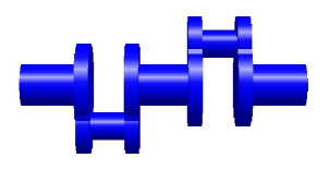
Figure 1: Crankshaft domain

Example 7.1

The numerical calculations are performed for the polynomial degree $p=2$, resulting in $N=13,986$ degrees of freedom. The largest block of $\mathbf{W}_{\mathcal{H}}$ has a size of $1,746^{2}$. In Figure 3, we compare the decrease of the upper bound $\left\|\mathbf{I}-\mathbf{W}^{\rm st}\mathbf{W}_{\mathcal{H}}\right\|_{2}$ of the relative error with the increase of the block-rank. Figure 3 shows the storage requirement for the computed $\mathcal{H}$-matrix approximation in MB. Storing the dense matrix would need $1,492$ MB. We observe exponential convergence in the block rank, even with a convergence behavior $\exp(-br^{1/2})$, which is faster than the rate of $\exp(-br^{1/4})$ guaranteed by Theorem 2.6. Moreover, we also observe exponential convergence of the error compared to the increase of required memory.

\psfrag{Error}[c][c]{\footnotesize Error}\psfrag{Block rank r }[c][c]{\footnotesize Block rank r}\psfrag{asd}[l][l]{\tiny$\exp(-2.2\,r^{1/2})$}\psfrag{jkl}[l][l]{\tiny$\left\|I-\mathbf{W}^{\rm st}W_{\mathcal{H}}\right\|_{2}$}\includegraphics[width=359.6442pt]{CS12r13986.eps}

Figure 2: Exponential convergence in block rank

\psfrag{Error}[c][c]{\footnotesize Error}\psfrag{Memory (MB)}[c][c]{\footnotesize Memory (MB)}\psfrag{asd}[l][l]{\tiny$\exp(-1.6\,r^{1/2})$}\psfrag{jkl}[l][l]{\tiny$\left\|I-\mathbf{W}^{\rm st}W_{\mathcal{H}}\right\|_{2}$}\includegraphics[width=359.6442pt]{CS12Memory13986.eps}

Figure 3: Exponential convergence in memory required

 

Example 7.2

We consider the case $p=3$, which leads to $N=31,466$ degrees of freedom. The largest block of $\mathbf{W}_{\mathcal{H}}$ has a size of $3,933^{2}$. Storing the dense matrix would need $7,608$ MB.

\psfrag{Error}[c][c]{\footnotesize Error}\psfrag{Block rank r }[c][c]{\footnotesize Block rank r}\psfrag{asd}[l][l]{\tiny$\exp(-1.7\,r^{1/2})$}\psfrag{jkl}[l][l]{\tiny$\left\|I-\mathbf{W}^{\rm st}W_{\mathcal{H}}\right\|_{2}$}\includegraphics[width=359.6442pt]{CS12r31466.eps}

Figure 4: Exponential convergence in block rank

\psfrag{Error}[c][c]{\footnotesize Error}\psfrag{Memory (MB)}[c][c]{\footnotesize Memory (MB)}\psfrag{asd}[l][l]{\tiny$\exp(-0.8\,r^{1/2})$}\psfrag{jkl}[l][l]{\tiny$\left\|I-\mathbf{W}^{\rm st}W_{\mathcal{H}}\right\|_{2}$}\includegraphics[width=359.6442pt]{CS12Memory31466.eps}

Figure 5: Exponential convergence in memory required

We observe in Figure 5 exponential convergence both in the block rank and in the memory.

References

• [Beb00] M. Bebendorf, Approximation of boundary element matrices, Numer. Math. 86 (2000), no. 4, 565–589.
• [Beb05a]  , Efficient inversion of Galerkin matrices of general second-order elliptic differential operators with nonsmooth coefficients, Math. Comp. 74 (2005), 1179–1199.
• [Beb05b]  , Hierarchical LU decomposition-based preconditioners for BEM, Computing 74 (2005), no. 3, 225–247.
• [Beb07]  , Why finite element discretizations can be factored by triangular hierarchical matrices, SIAM J. Numer. Anal. 45 (2007), no. 4, 1472–1494.
• [Beb12]  , Another software library on hierarchical matrices for elliptic differential equations (AHMED), http://bebendorf.ins.uni-bonn.de/AHMED.html (2012).
• [BG05] S. Börm and L. Grasedyck, Hybrid cross approximation of integral operators, Numer. Math. 101 (2005), no. 2, 221–249.
• [BH03] M. Bebendorf and W. Hackbusch, Existence of $\mathcal{H}$-matrix approximants to the inverse FE-matrix of elliptic operators with $L^{\infty}$-coefficients, Numer. Math. 95 (2003), no. 1, 1–28.
• [Bör10a] S. Börm, Approximation of solution operators of elliptic partial differential equations by $\mathcal{H}$- and $\mathcal{H}^{2}$-matrices, Numer. Math. 115 (2010), no. 2, 165–193.
• [Bör10b]  , Efficient numerical methods for non-local operators, EMS Tracts in Mathematics, vol. 14, European Mathematical Society (EMS), Zürich, 2010.
• [BS02] S. C. Brenner and L. R. Scott, The mathematical theory of finite element methods, Texts in Applied Mathematics, vol. 15, Springer-Verlag, New York, 2002.
• [DFG+01] W. Dahmen, B. Faermann, I. G. Graham, W. Hackbusch, and S. A. Sauter, Inverse inequalities on non-quasiuniform meshes and application to the mortar element method, Math. Comp. 73 (2001), 1107–1138.
• [DKP+08] Leszek Demkowicz, Jason Kurtz, David Pardo, Maciej Paszyński, Waldemar Rachowicz, and Adam Zdunek, Computing with $hp$-adaptive finite elements. Vol. 2, Chapman & Hall/CRC Applied Mathematics and Nonlinear Science Series, Chapman & Hall/CRC, Boca Raton, FL, 2008, Frontiers: Three dimensional elliptic and Maxwell problems with applications.
• [FMP12] M. Faustmann, J. M. Melenk, and D. Praetorius, A new proof for existence of $\mathcal{H}$-matrix approximants to the inverse of FEM matrices: the Dirichlet problem for the Laplacian, ASC Report 51/2012, Institute for Analysis and Scientific Computing, Vienna University of Technology, Wien (2012).
• [FMP13a]  , Existence of $\mathcal{H}$-matrix approximants to the inverse of BEM matrices: the simple-layer operator, ASC Report 20/2013, Institute for Analysis and Scientific Computing, Vienna University of Technology, Wien (2013).
• [FMP13b]  , $\mathcal{H}$-matrix approximability of the inverse of FEM matrices, ASC Report 37/2013, Institute for Analysis and Scientific Computing, Vienna University of Technology, Wien (2013).
• [GH03] L. Grasedyck and W. Hackbusch, Construction and arithmetics of $\mathcal{H}$-matrices, Computing 70 (2003), no. 4, 295–334.
• [GHS05] I. G. Graham, W. Hackbusch, and S. A. Sauter, Finite elements on degenerate meshes: inverse-type inequalities and applications, IMA J. Numer. Anal. 25 (2005), no. 2, 379–407.
• [GKLB09] L. Grasedyck, R. Kriemann, and S. Le Borne, Domain decomposition based $\mathcal{H}$-LU preconditioning, Numer. Math. 112 (2009), no. 4, 565–600.
• [GR97] L. Greengard and V. Rokhlin, A new version of the fast multipole method for the Laplace in three dimensions, Acta Numerica 1997, Cambridge University Press, 1997, pp. 229–269.
• [Gra01] L. Grasedyck, Theorie und Anwendungen Hierarchischer Matrizen, Ph.D. thesis, Universität Kiel, 2001.
• [Gra05]  , Adaptive recompression of $\mathcal{H}$-matrices for BEM, Computing 74 (2005), no. 3, 205–223.
• [Hac99] W. Hackbusch, A sparse matrix arithmetic based on $\mathcal{H}$-matrices. Introduction to $\mathcal{H}$-matrices, Computing 62 (1999), no. 2, 89–108.
• [Hac09]  , Hierarchische Matrizen: Algorithmen und Analysis, Springer, 2009.
• [HJ13] R.A. Horn and Ch.R. Johnson, Matrix analysis, second ed., Cambridge University Press, Cambridge, 2013.
• [HKS00] W. Hackbusch, B. Khoromskij, and S. A. Sauter, On $\mathcal{H}^{2}$-matrices, Lectures on Applied Mathematics (2000), 9–29.
• [HN89] W. Hackbusch and Z.P. Nowak, On the fast matrix multiplication in the boundary element method by panel clustering, Numer. Math. 54 (1989), 463–491.
• [HS93] W. Hackbusch and S.A. Sauter, On the efficient use of the Galerkin method to solve Fredholm integral equations, Proceedings of ISNA ’92—International Symposium on Numerical Analysis, Part I (Prague, 1992), vol. 38, 1993, pp. 301–322.
• [KS99] G.E. Karniadakis and S.J. Sherwin, Spectral/hp element methods for cfd, Oxford University Press, 1999.
• [Neč67] J. Nečas, Les méthodes directes en théorie des équations elliptiques, Masson et Cie, Éditeurs, Paris, 1967.
• [NH88] Z.P. Novak and W. Hackbusch, Complexity of the method of panels, Computational processes and systems, No. 6 (Russian), “Nauka”, Moscow, 1988, pp. 233–244.
• [NS74] Joachim A. Nitsche and Alfred H. Schatz, Interior estimates for Ritz-Galerkin methods, Math. Comp. 28 (1974), 937–958.
• [Rat98] A. Rathsfeld, A wavelet algorithm for the boundary element solution of a geodetic boundary value problem, Comput. Methods Appl. Mech. Engrg. 157 (1998), no. 3-4, 267–287, Seventh Conference on Numerical Methods and Computational Mechanics in Science and Engineering (NMCM 96) (Miskolc).
• [Rat01]  , On a hierarchical three-point basis in the space of piecewise linear functions over smooth surfaces, Problems and methods in mathematical physics (Chemnitz, 1999), Oper. Theory Adv. Appl., vol. 121, Birkhäuser, Basel, 2001, pp. 442–470.
• [Rok85] V. Rokhlin, Rapid solution of integral equations of classical potential theory, J. Comput. Phys. 60 (1985), 187–207.
• [Sau92] S.A. Sauter, Über die effiziente Verwendung des Galerkinverfahrens zur Lösung Fredholmscher Integralgleichungen, Ph.D. thesis, Universität Kiel, 1992.
• [SBA+15] W. Smigaj, T. Betcke, S. R. Arridge, J. Phillips, and M. Schweiger, Solving boundary integral problems with BEM++, ACM Transactions on Mathematical Software (to appear (2015)).
• [Sch97] J. Schöberl, NETGEN - An advancing front 2D/3D-mesh generator based on abstract rules, Comput.Visual.Sci (1997), no. 1, 41–52.
• [Sch98a] R. Schneider, Multiskalen- und Wavelet-Matrixkompression: Analysisbasierte Methoden zur effizienten Lösung großer vollbesetzter Gleichungssysteme, Advances in Numerical Mathematics, Teubner, 1998.
• [Sch98b] Ch. Schwab, $p$- and $hp$-finite element methods, Numerical Mathematics and Scientific Computation, The Clarendon Press Oxford University Press, New York, 1998, Theory and applications in solid and fluid mechanics.
• [Sch06] Robert Schrittmiller, Zur Approximation der Lösungen elliptischer Systeme partieller Differentialgleichungen mittels Finiter Elemente und {\mathcal{\char 72\relax}}-Matrizen, Ph.D. thesis, Technische Universität München, 2006.
• [SS11] S.A. Sauter and Ch. Schwab, Boundary element methods, Springer Series in Computational Mathematics, vol. 39, Springer-Verlag, Berlin, 2011.
• [Ste70] E.M. Stein, Singular integrals and differentiability properties of functions, Princeton University Press, 1970.
• [Ste08] O. Steinbach, Numerical approximation methods for elliptic boundary value problems, Springer, New York, 2008.
• [SZ90] L. R. Scott and S. Zhang, Finite element interpolation of nonsmooth functions satisfying boundary conditions, Math. Comp. 54 (1990), no. 190, 483–493.
• [Tau03] J. Tausch, Sparse BEM for potential theory and Stokes flow using variable order wavelets, Comput. Mech. 32 (2003), no. 4-6, 312–318.
• [TW03] J. Tausch and J. White, Multiscale bases for the sparse representation of boundary integral operators on complex geometry, SIAM J. Sci. Comput. 24 (2003), no. 5, 1610–1629.
• [Tyr00] E.E. Tyrtyshnikov, Incomplete cross approximation in the mosaic-skeleton method, Computing 64 (2000), no. 4, 367–380, International GAMM-Workshop on Multigrid Methods (Bonn, 1998).
• [vPSS97] T. von Petersdorff, Ch. Schwab, and R. Schneider, Multiwavelets for second-kind integral equations, SIAM J. Numer. Anal. 34 (1997), no. 6, 2212–2227.
• [Wah91] L. Wahlbin, Local behavior in finite element methods, Handbook of numerical analysis. Volume II: Finite element methods (Part 1) (P.G. Ciarlet and J.L. Lions, eds.), North Holland, 1991, pp. 353–522.