Space-Time Models based on Random Fields with Local Interactions

Abstract

The analysis of space-time data from complex, real-life phenomena requires the use of flexible and physically motivated covariance functions. In most cases, it is not possible to explicitly solve the equations of motion for the fields or the respective covariance functions. In the statistical literature, covariance functions are often based on mathematical constructions. We propose deriving space-time covariance functions by solving “effective equations of motion”, which can be used as statistical representations of systems with diffusive behavior. In particular, we propose using the linear response theory to formulate space-time covariance functions based on an equilibrium effective Hamiltonian. The effective space-time dynamics are then generated by a stochastic perturbation around the equilibrium point of the classical field Hamiltonian leading to an associated Langevin equation. We employ a Hamiltonian which extends the classical Gaussian field theory by including a curvature term and leads to a diffusive Langevin equation. Finally, we derive new forms of space-time covariance functions.

Keywords: fluctuation dissipation theorem; interpolation; simulation; space-time system; maximum entropy.

1 Introduction

Covariance functions play a significant role in the analysis of space-time data with geostatistical and machine learning methods [46, 45, 7], in inverse modelling [48], and in data assimilation [34]. Thus, there is active interest in applications of space-time data analysis and the development of new covariance models [7, 1]. Space-time covariance functions commonly used are straightforward extensions of purely spatial models (e.g., exponential, Gaussian) and constructions based on linear mixtures [39]. More complex models are generated using mathematical arguments, e.g. permissibility conditions [40] and simplifying assumptions such as separability of space and time components without clear physical motivation for the functional form or the parameters. Several authors have proposed more realistic, non-separable covariance models [8, 36, 9]. Simple space-time covariance models are determined by the variance and constant correlation length and correlation time. In purely spatial cases, richer parametric families such as the Whittle-Matérn covariance model [15, 20] or the Spartan covariance functions [25, 24, 27] offer more flexibility. The former is derived from a fractional stochastic partial differential equation driven by white noise [53, 38]. The latter is obtained from a Gaussian field theory with a curvature term which also leads to a fourth-order stochastic partial differential equation [26, 27].

There is a long history of ideas from physics that find applications in information theory and data analysis, including the maximum entropy formalism developed by Jaynes [32], more recently the Bayesian field theory [37], and machine learning applications of the variational approximation [22]. The connection between statistical physics and space-time statistics on the other hand has not been duly appreciated, albeit the former can provide useful models for the analysis of space-time data. In statistical physics the literature on space-time fields and correlation functions is extensive [14]. For example, the Gaussian model of classical field theory is equivalent to a Gaussian random field with a specific covariance function [35, 43].

A formal difference between random fields in statistical field theories and those in spatial statistics is that the former are defined by means of local interactions, whereas the latter are defined by means of covariance matrices [5, 6]. Both approaches are formally equivalent provided that the covariance function of the local interaction model can be explicitly expressed. The interaction-based formalism has several advantages for parameter estimation, interpolation and simulation which derive from the sparseness of the inverse covariance matrix in the local interaction representation [28, 50]. Spartan Spatial Random Fields (SSRFs) are based on the local interaction framework in the static (time-independent) case. SSRFs admit explicit relations for the covariance function in one, two, and three dimensions [25, 24, 11, 10, 27]. A similar framework was independently proposed by Farmer [12]. More recently, covariance functions similar to SSRF were derived for meteorological applications from polynomials of the diffusion operator [58, 56].

In statistical physics, a coarse-grained Hamiltonian determines the relative probabilities of different field configurations for near-equilibrium systems. Excursions from equilibrium leading to dynamic fluctuations follow by perturbing the system with noise. The dynamic response of the system is determined by a stochastic partial differential equation, also known as Langevin equation, which can be derived in the framework of linear response theory [18]. The correlation functions are shown to obey the fluctuation-dissipation theorem, which connects them to respective susceptibility functions [42]. In physics, this approach has been applied to study dynamic critical phenomena [23, 47].

The physical insight provided by the the fluctuation-dissipation theorem is that the fluctuations of the unperturbed system contain information about the response to external perturbations that drive the system away from equilibrium. This formalism, to our knowledge, has not been applied to generate space-time covariance functions. Our goal in this paper is to show that effective Hamiltonians with local interactions, which are successfully used in spatial data analysis, can be extended to space-time random fields. This contribution is part of an ongoing effort to transfer ideas from statistical physics to space-time data analysis [25, 26, 10, 24, 28, 27]. Using the theory of linear response, we show that the local interaction framework leads to explicit forms for new space-time covariance functions.

The remainder of the paper is structured as follows: In Section 2 we present mathematical background on Gaussian random fields. Section 3 reviews local interaction random fields and demonstrates that the so-called Spartan spatial random field model is derived from the principle of maximum entropy. Section 4 briefly presents linear response theory focusing on the calculation of correlation functions. In Section 5 we use linear response theory to derive equations of motion for space-time SSRF covariances, and we obtain an explicit equation for the SSRF spectral density. Section 6 gives a standard derivation of space-time covariances from Langevin equations. This leads to a general equation for the space-time covariance function of fields driven by colored noise and recaptures the results of the previous Section in the SSRF case with Gaussian white noise. In Section 7 we present explicit equations for SSRF space-time covariance functions. Finally, we present our conclusions in Section 8.

2 Mathematical Preliminaries

In the following, we focus on Gaussian space-time random fields. These can be used to model more complicated distributions in the Bayesian framework of Gaussian random processes [45]. A space-time random field (STRF) $X({\bf s},t;\omega)\in\mathbb{R}$ where $({\bf s},t)\in\mathbb{R}^{d}\times\mathbb{R}$ and $\omega\in\Omega$ is defined as a mapping from the probability space $(\Omega,A,P)$ into the space of real numbers so that for each fixed coordinate $({\bf s},t)$, $X({\bf s},t;\omega)$ is a measurable function of $\omega$ [5]. An STRF involves by definition many possible states indexed by $\omega$ [5, 55]. In the following, we drop the state index $\omega$ for simplicity; instead, we use the symbol $\omega$ for the cyclical frequency in Fourier transforms. The states (realizations) of the STRF are denoted by the real-valued scalar functions $x({\bf s},t)$. In the following, $\Phi\left[X({\bf s},t)\right]$ denotes a functional of the STRF $X({\bf s},t)$ that takes unique values for each realization $x({\bf s},t)$.

The expectation over the ensemble of STRF states is denoted by the angle brackets $\left\langle{\,\cdot}\,\right\rangle.$ Hence, the covariance function is given by

$$C_{{\rm x}}({\bf s},t;{{\bf s}^{\prime},t^{\prime}}) = \left\langle{\,X({\bf s}^{\prime},t^{\prime})\,X({\bf s},t)}\,\right\rangle-\left\langle{\,X({\bf s}^{\prime},t^{\prime})}\,\right\rangle\,\left\langle{\,X({\bf s},t)}\,\right\rangle.$$ (1)

An STRF is called statistically stationary in the weak sense (or simply stationary for brevity), if its expectation is constant and its covariance function depends purely on the spatial and temporal lags, ${\bf r}$ and $\tau$, respectively. For simplicity, since we aim to calculate space-time covariance functions, we assume a zero-mean STRF, i.e. $\left\langle{\,X({\bf s},t)}\,\right\rangle=0.$ The STRF variance will be denoted by $\sigma^{2}$. Furthermore, a stationary random field is called statistically isotropic if its covariance function depends only on the Euclidean distance but not the direction vector. In the following we focus on statistically isotropic STRFs.

In the spectral domain, we use the wavevector ${\bf k}$ to denote the spatial frequency and $\omega$ to denote the cyclic frequency with respect to time. For a given function $x({\bf s},t)$ with space and time dependence, we will use $\tilde{x}({\bf k},t)$ to denote the spatial (i.e., with respect to the space variable) Fourier transform and $\tilde{x}({\bf k},\omega)$ the full Fourier transform with respect to both space and time. The pairs of the direct and inverse Fourier transforms, respectively, are defined as follows:

$$\tilde{x}({\bf k},t)=\mathcal{F}_{{\bf s}}[x]({\bf k},t)=\int_{\mathbb{R}^{d}}d{\bf s}\,\mathrm{e}^{-\jmath\,{\bf k}\cdot{\bf r}}\,x({\bf s},t),$$ (2a)

$$x({\bf s},t)=\mathcal{F}_{{\bf k}}^{-1}[\tilde{x}]({\bf s},t)=\frac{1}{(2\pi)^{d}}\int_{\mathbb{R}^{d}}d{\bf k}\,\mathrm{e}^{\jmath\,{\bf k}\cdot{\bf r}}\,\tilde{x}({\bf k},t),$$ (2b)

$$\tilde{x}({\bf k},\omega)=\mathcal{F}_{{\bf s},t}[x]({\bf k},\omega)=\int_{\mathbb{R}^{d}}d{\bf s}\,\int_{-\infty}^{\infty}dt\,\mathrm{e}^{-\jmath\,({\bf k}\cdot{\bf r}+\omega\,t)}\,x({\bf s},t),$$ (2c)

$$x({\bf s},t)=\mathcal{F}_{{\bf k},\omega}^{-1}[\tilde{x}]({\bf s},t)=\frac{1}{(2\pi)^{d+1}}\int_{\mathbb{R}^{d}}d{\bf k}\,\int_{-\infty}^{\infty}d\omega\,\mathrm{e}^{\jmath\,({\bf k}\cdot{\bf r}+\omega\,t)}\,\tilde{x}({\bf k},\omega).$$ (2d)

3 Local Interaction Random Fields

Time-independent random fields represent the long-time, i.e., equilibrium, configurations of dynamic variables. They also model “quenched randomness” which characterizes the structure of geological media and is a key factor for subsurface physical processes [5]. Static random fields can be defined in terms of a “pseudo-energy” functional $\mathcal{H}[x({\bf s})]$ which assigns different “energy” levels, and subsequently different probabilities, to different configurations $x({\bf s})$. In the following, we will assume that the energy functional takes real, non-negative values. The most probable configuration of the spatial random field minimizes $\mathcal{H}[x({\bf s})]$.

The joint probability density function (pdf) of the equilibrium spatial random field $X({\bf s};\omega)$ is determined from the functional $\mathcal{H}[x({\bf s})]$. The joint pdf for the realization (state) $x({\bf s})$ is proportional to $\exp[-\mathcal{H}[x({\bf s})]$, i.e.,

$$f_{\mathrm{eq}}\left[x({\bf s})\right]=\frac{1}{Z}\,\mathrm{e}^{-\mathcal{H}\left[x({\bf s})\right]},$$

where the partition function $Z$ is given by the following functional integral [17, 13]

$$Z=\int\mathcal{D}x({\bf s})\,\mathrm{e}^{-\mathcal{H}\left[x({\bf s})\right]}.$$

The functional integral is the continuum limit of the discrete representation $\mathcal{D}x({\bf s})=\lim_{n\rightarrow\infty}\prod_{i=1}^{n}dx_{i}$, where the vector $(x_{1},\ldots,x_{n})^{T}$ represents a discretization of the continuum state $x({\bf s})$ at $n$ points. Note that whereas $Z$ may diverge for $n\rightarrow\infty$, the SRF statistical moments are nonetheless well defined. For example, the covariance is given by the following functional integral

$$\left\langle{\,X({{\bf s}}_{1})\,X({{\bf s}}_{2})}\,\right\rangle=\frac{1}{Z}\,\int\mathcal{D}x({\bf s})\,x({{\bf s}}_{1})\,x({{\bf s}}_{2})\,\mathrm{e}^{-\mathcal{H}[x({\bf s})]}.$$ (3)

In statistical mechanics, the $\mathcal{H}[x({\bf s})]$ for a given system is obtained from kinetic and potential energy terms that reflect the motion and interactions of microscopic constituents. In the case of macroscopic random fields $X({\bf s},t)$, the dynamics may not be fully known or solvable. Then, $\mathcal{H}[x({\bf s})]$ represents an effective functional that incorporates fictitious interactions defined by means of derivatives of the field realizations. Hence, $\mathcal{H}[x({\bf s})]$ may represent a sufficiently flexible heuristic functional and not a first-principles Hamiltonian.

3.1 Maximum Entropy Formulation of Spartan Spatial Random Fields

Based on the concept of the effective energy functional, the Spartan spatial random field model was proposed [25, 24, 28, 27]. This model is an extension of the classical Gaussian field theory [35] which incorporates a square curvature term. The respective energy functional is given by

$$\mathcal{H}_{\mathrm{f}gc}\left[x({\bf s})\right] = \frac{1}{{2\eta_{0}\xi^{d}}}\int_{\mathbb{R}^{d}}d{\bf s}\,\left\{\left[x({\bf s})\right]^{2}+\eta_{1}\,\xi^{2}\left[{\nabla x({\bf s})}\right]^{2}+\xi^{4}\,\left[{\nabla^{2}\,x({\bf s})}\right]^{2}\right\}.$$ (4)

In the above, $\eta_{0}$ represents a scale coefficient, $\eta_{1}$ a rigidity coefficient, and $\xi$ a characteristic length; $\nabla$ stands for the gradient and $\nabla^{2}$ for the Laplace differential operator. The energy functional $\mathcal{H}_{\rm fgc}\left[x({\bf s})\right]$ generates Gaussian, zero-mean, stationary random fields. As in classical field theory, a frequency cutoff is required for differentiability of the field states [59]. In the absence of such a cutoff, the high-frequency contributions lead to random fields that are mean-square continuous but non-differentiable in $d=2,3$ [24]. Explicit expressions for the covariance functions in $d=1,2,3$ at the limit of infinite cutoff are derived in [24, 27]. The use of (4) in spatial data analysis requires the estimation of the coefficients $\eta_{0}$, $\eta_{1}$ and $\xi$ from the data.

The pdf with energy functional (4) can be derived using the principle of maximum entropy [32]. The main idea underlying maximum entropy is that the pdf is determined by maximizing the entropy of the system given constraints imposed by the data. Furthermore, it is assumed that the data constraints are equal to the respective expectations over the pdf.

Let us define the integrals $S_{i}[x({\bf s})$, $i=0,1,2$, by

$${S_{0}\left[x({\bf s})\right]}:= {\int d{\bf s}\,x^{2}({\bf s})},$$ (5a)

$${S_{1}\left[x({\bf s})\right]}:= {\int d{\bf s}\,[\nabla x({\bf s})]^{2}},$$ (5b)

$${S_{2}\left[x({\bf s})\right]}:= {\int d{\bf s}\,[\nabla^{2}x({\bf s})]^{2}},$$ (5c)

In addition, we assume that the expectations $\left\langle{\,S_{i}[x({\bf s})]}\,\right\rangle$ can be estimated from the data. If we possess only one realization, e.g., $x^{\ast}({\bf s})$, the above assumption requires that the system is ergodic with respect to the constraints, i.e., $\left\langle{\,S_{i}[x({\bf s})]}\,\right\rangle=S_{i}[x^{\ast}({\bf s})]$. Then, the maximum entropy pdf conditional on these constraints is given by

$$f_{\mathrm{eq}}\left[x({\bf s})\right]=\mathrm{e}^{-\mu-\lambda_{0}S_{0}\left[x({\bf s})\right]-\lambda_{1}S_{1}\left[x({\bf s})\right]-\lambda_{2}S_{2}\left[x({\bf s})\right]}.$$ (6)

The constant $\mu$ normalizes the pdf, i.e., $Z=\exp(\mu)$, whereas the constants $\lambda_{i}$, $i=0,1,2$ are in principle obtained by solving the system of the three equations $\left\langle{\,S_{i}[x({\bf s})]}\,\right\rangle=S_{i}[x({\bf s})]$. Note that (6) is equivalent to (4) if $\lambda_{0}={1}/{2\eta_{0}\xi^{d}}$, $\lambda_{1}={\eta_{1}\xi^{2-d}}/{2\eta_{0}}$, and $\lambda_{2}={\xi^{4-d}}/{2\eta_{0}}$.

For data sampled on discrete supports, the $S_{i}\left[x({\bf s})\right]$ are replaced by discretized estimators $\hat{S}_{i}({\bf x}^{\ast})$, that involve the sample values $({\bf x}^{\ast})^{T}=(x_{1}^{\ast},\ldots x_{N}^{\ast})$. For example, on a regular grid the derivatives are replaced by respective finite differences which thus implement the high-frequency cutoff [25]. On irregular grids, estimators can be constructed using kernel functions [10, 51]. Then, the estimation of the model parameters is reduced to the solution of the following moment equations

$$\hat{S}_{0}({\bf x}^{\ast})= \int_{-\infty}^{\infty}dx_{1}\ldots\int_{-\infty}^{\infty}dx_{N}\,\hat{S}_{0}({\bf x})\,\mathrm{e}^{-\mu-\lambda_{0}\hat{S}_{0}({\bf x})-\lambda_{1}\hat{S}_{1}({\bf x})-\lambda_{2}\hat{S}_{2}({\bf x})},$$ (7a)

$$\hat{S}_{1}({\bf x}^{\ast})= \int_{-\infty}^{\infty}dx_{1}\ldots\int_{-\infty}^{\infty}dx_{N}\,\hat{S}_{1}({\bf x})\,\mathrm{e}^{-\mu-\lambda_{0}\hat{S}_{0}({\bf x})-\lambda_{1}\hat{S}_{1}({\bf x})-\lambda_{2}\hat{S}_{2}({\bf x})},$$ (7b)

$$\hat{S}_{2}({\bf x}^{\ast})= \int_{-\infty}^{\infty}dx_{1}\ldots\int_{-\infty}^{\infty}dx_{N}\,\hat{S}_{2}({\bf x})\,\mathrm{e}^{-\mu-\lambda_{0}\hat{S}_{0}({\bf x})-\lambda_{1}\hat{S}_{1}({\bf x})-\lambda_{2}\hat{S}_{2}({\bf x})}.$$ (7c)

4 Dynamic Correlations

If a perturbation drives the system away from the equilibrium and the deviation is small, the equilibrium fluctuations determine the non-equilibrium response. This idea is exploited in statistical mechanics by means of the linear response theory [23].

4.1 Susceptibility Function

The theory of linear response focuses on small perturbations of the field $X({\bf s},t)$ around the equilibrium state which are caused by an external field $h({\bf s},t)$. If we define by $\left\langle{\cdot}\right\rangle_{0}$ the expectation over the equilibrium distribution and by $\left\langle{\,\cdot}\,\right\rangle$ the non-equilibrium expectation, the response of the system to the external field can be expressed as follows in terms of the susceptibility function $\chi({\bf s}-{\bf s}^{\prime};t-t^{\prime})$ and the following convolution equation

$$\left\langle{\,X({\bf s},t)}\,\right\rangle=\left\langle{X({\bf s},t)}\right\rangle_{0}+\int_{-\infty}^{t}dt^{\prime}\int_{\mathbb{R}^{d}}d{{\bf s}}^{\prime}\,\chi({\bf s}-{\bf s}^{\prime};t-t^{\prime})\,h({\bf s}^{\prime},t^{\prime}).$$ (8)

For large perturbations, the response should also include nonlinear terms.

Since the difference $\left\langle{\,X({\bf s},t)}\,\right\rangle-\left\langle{X({\bf s},t)}\right\rangle_{0}=\left\langle{\,X^{\prime}({\bf s},t)}\,\right\rangle$ corresponds to the expectation of the non-equilibrium fluctuation, Eq. (8) implies that the susceptibility is given by the following functional derivative

$${\chi}({\bf s}-{\bf s}^{\prime},t-t^{\prime})=\lim_{h({{\bf s}^{\prime},t^{\prime}})\rightarrow 0}\frac{\delta\left\langle{\,{X^{\prime}}({\bf s},t)}\,\right\rangle}{\delta{h}({{\bf s}^{\prime},t^{\prime}})}.$$ (9)

In the above, $\delta(\cdot)/\delta h({{\bf s}^{\prime},t^{\prime}})$ represents the functional derivative, which is defined by means of $\delta h({\bf s},t)/\delta h({{\bf s}^{\prime},t^{\prime}})=\delta({\bf s}-{\bf s}^{\prime})\,\delta(t-t^{\prime})$. The limit $h({{\bf s}^{\prime},t^{\prime}})\rightarrow 0$ is taken in order to ensure that nonlinear terms vanish.

Let $\tilde{X^{\prime}}({\bf k},\omega)$ and $\tilde{h}({\bf k},\omega)$ represent the Fourier transforms of the STRF fluctuation and the external field which are given by (2). The Fourier transform of the susceptibility function is then given by the following limit

$$\tilde{\chi}({\bf k},\omega)=\lim_{\tilde{h}\rightarrow 0}\frac{\delta\left\langle{\,\tilde{X^{\prime}}({\bf k},\omega)}\,\right\rangle}{\delta\tilde{h}({\bf k},\omega)}.$$ (10)

The susceptibility function is used in physical applications to describe the system’s response to measurable external fields (e.g., electric or magnetic fields). In the analysis of spatial data, however, the external field does not necessarily represent a physical reality; hence, the notion of susceptibility has not found wide applicability. Nevertheless, we suggest that there are potential applications of the susceptibility concept, since the analysis of spatial fields often involves auxiliary variables [52], which essentially represent external fields. For example, the elevation is an auxiliary variable that has significant impact on rainfall; thus, it makes sense to consider the susceptibility of the rainfall field to the elevation of a particular site.

4.2 Langevin Equations

Within the framework of linear response theory, the STRF dynamics is derived from the equilibrium energy functional and the noise field that drives deviations from the equilibrium by means of the following Langevin equation [31, 18]

$$\frac{\partial X({\bf s},t)}{\partial t}=-\Gamma\,\left.\frac{\delta\mathcal{H}[x({\bf s})]}{\delta x({\bf s})}\right|_{x({\bf s})=X({\bf s},t)}+\zeta({\bf s},t),$$ (11)

where $\Gamma$ is a diffusion coefficient, $\delta[.]/\delta x({\bf s})$ denotes the functional derivative with respect to the field state, and $\zeta({\bf s},t)$ is the noise field. The latter is typically Gaussian white noise with $\left\langle{\,\zeta({\bf s},t)}\,\right\rangle=0$ and variance equal to $D$, i.e.,

$$\left\langle{\,\zeta({\bf s},t)\,\zeta({{\bf s}^{\prime},t^{\prime}})}\,\right\rangle=D\,\delta({\bf s}-{\bf s}^{\prime})\,\delta(t-t^{\prime}).$$ (12)

Equation (11) links the rate of change of the field state $x({\bf s},t)$ to an equilibrium-restoring velocity that depends on $\mathcal{H}[x({\bf s})]$ and a random velocity given by the noise term. For example, if $\mathcal{H}[x({\bf s})]$ is given by the Ginzburg-Landau effective action, then (11) is known as the time-dependent Ginzburg-Landau equation [35, p.192]. In the following, we will denote the restoring velocity for a given random field state by

$$V[x({\bf s})]:=-\Gamma\,\frac{\delta\mathcal{H}[x({\bf s})]}{\delta x({\bf s})},$$ (13)

and $V[X({\bf s},t)]$ will denote the respective functional of the random field $X({\bf s},t)$.

4.3 Fokker-Planck Equation

The pdf of the STRF $X({\bf s},t)$ that is governed by the Langevin equation (11) is the solution of the following Fokker-Planck equation [18]

$$\frac{\partial f\left[x({\bf s},t)\right]}{\partial t}=\int_{\mathbb{R}^{d}}d{{\bf s}}^{\prime}\,\frac{\delta}{\delta x({\bf s},t)}\left[-V\left[x({\bf s}^{\prime},t)\right]\,f_{X}\left[x({\bf s},t)\right]+\frac{D}{2}\frac{\delta f_{X}\left[x({\bf s},t)\right]}{\delta x({{\bf s}}^{\prime},t)}\right]$$ (14)

The equilibrium (time-independent) pdf is the asymptotic limit (as $t\rightarrow\infty$) of the solution of the above Fokker-Planck equation:

$$f_{\mathrm{eq}}\left[x({\bf s})\right]\propto\exp\left\{-\frac{2\Gamma\,\mathcal{H}\left[x({\bf s})\right]}{D}\right\}.$$ (15)

The Fokker-Planck equation may not admit an explicit solution; however, for many applications in spatial data analysis it is sufficient to know the covariance of the random field, since the fluctuations often follow the Gaussian law, whereas in other cases the data can be transformed by means of nonlinear transformations to approximately fit the Gaussian law [52].

4.4 Equation of Motion for the Covariance

To obtain the equation of motion (EOM) for the covariance function, we follow the approach described in [42, pp. 120-121]. First, we assume that $t>t^{\prime}$ without loss of generality. We use the covariance definition (1), we replace the time derivative of $X({\bf s},t)$ with (11), and then replace $x({\bf s},t)$ with the random fields $X({\bf s},t)$. These steps lead to the following equation

$$\frac{\partial C_{{\rm x}}({\bf s},t;{{\bf s}^{\prime},t^{\prime}})}{\partial t}=\left\langle{\,\left[V[X({\bf s},t)]+\zeta({\bf s},t;\omega)\right]\,X({{\bf s}}^{\prime},t^{\prime})}\,\right\rangle.$$ (16)

The right hand side of the above equation involves the term $\left\langle{\,\zeta({\bf s},t;\omega)\,X({{\bf s}}^{\prime},t^{\prime})}\,\right\rangle$. The principle of causality, however, implies that the noise at time $t$ can not influence the field at the earlier time $t^{\prime}$. Hence, noise-field cross correlation is dropped, and we obtain the following EOM for the covariance:

$$\frac{\partial C_{{\rm x}}({\bf s},t;{{\bf s}^{\prime},t^{\prime}})}{\partial t}=\left\langle{\,V[X({\bf s},t)]\,X({{\bf s}}^{\prime},t^{\prime})}\,\right\rangle.$$ (17)

Let us now assume that $t\leq t^{\prime}$ then since we can not reason that causality causes the noise-field cross correlation to vanish the EOM for the covariance will be given by:

$$\frac{\partial C_{{\rm x}}({\bf s},t;{{\bf s}^{\prime},t^{\prime}})}{\partial t}=\left\langle{\,V[X({\bf s},t)]\,X({{\bf s}}^{\prime},t^{\prime})}\,\right\rangle+\left\langle{\,\zeta({\bf s},t;\omega)\,X({{\bf s}^{\prime},t^{\prime}};\omega)}\,\right\rangle.$$ (18)

Moreover from (17) the partial derivative of the covariance with respect to $t^{\prime}$ will be given by:

$$\frac{\partial C({\bf s},t;{\bf s}^{\prime},t^{\prime})}{\partial t^{\prime}}=\left\langle{\,V[X({{\bf s}}^{\prime},t^{\prime})]\,X({\bf s},t)}\,\right\rangle.$$ (19)

Next, we subtract each side of the equation for $\partial C_{{\rm x}}({\bf s},t;{{\bf s}^{\prime},t^{\prime}})/\partial t^{\prime}$ from the respective side of (18) for $\partial C_{{\rm x}}({\bf s},t;{{\bf s}^{\prime},t^{\prime}})/\partial t$. At this point we use the stationarity property, i.e., that the covariance is a function only of the lag $t-t^{\prime}$, which implies $\partial C_{{\rm x}}({\bf s},t;{{\bf s}^{\prime},t^{\prime}})/\partial t^{\prime}=-\partial C_{{\rm x}}({\bf s},t;{{\bf s}^{\prime},t^{\prime}})/\partial t.$ These operations lead to the following equation for the covariance rate

$$2\,\frac{\partial C_{{\rm x}}({\bf s},t;{{\bf s}^{\prime},t^{\prime}})}{\partial t}= ~{}\left\langle{\,V[X({\bf s},t)]\,X({{\bf s}^{\prime},t^{\prime}};\omega)}\,\right\rangle$$

$$-\left\langle{\,V[X({{\bf s}}^{\prime},t^{\prime})]\,X({\bf s},t;\omega)}\,\right\rangle$$

$$+\left\langle{\,\zeta({\bf s},t;\omega)\,X({{\bf s}^{\prime},t^{\prime}};\omega)}\,\right\rangle.$$ (20)

Using time and space translation invariance, the first two averages on the left hand side cancel each other. Combining Equations (17), (18) and (4.4) we obtain

$$\frac{\partial C({\bf s},t;{\bf s}^{\prime},t^{\prime})}{\partial t}=\mathrm{sign}(t-t^{\prime})\left\langle{\,V[X({{\bf s}}^{\prime},t^{\prime})]\,X({\bf s},t)}\,\right\rangle.$$ (21)

4.5 The Fluctuation-Dissipation theorem

The fluctuation-dissipation theorem links the covariance and the susceptibility functions [23]. For $t>t^{\prime}$ from (4.4) it is straightforward that:

$$2\,\frac{\partial C_{{\rm x}}({\bf s},t;{{\bf s}^{\prime},t^{\prime}})}{\partial t}=\left\langle{\,\zeta({{\bf s}^{\prime},t^{\prime}};\omega)\,X({\bf s},t;\omega)}\,\right\rangle.$$ (22)

The term in the right hand side of can be evaluated by means of the Furutsu-Novikov theorem [16, 44]. The latter states that if $\zeta({\bf s},t;\omega)$ is a Gaussian process and $\phi[X({\bf s},t)]$ is a function of $X({\bf s},t)$ then the following identity holds

$$\left\langle{\,\phi[X({\bf s},t)]\,\zeta({{\bf s}^{\prime},t^{\prime}};\omega)}\,\right\rangle= \int d{{\bf s}}^{\prime\prime}\int dt^{\prime\prime}\,\left\langle{\,\frac{\delta\phi[X({\bf s},t)]}{\delta\zeta({{\bf s}^{\prime\prime},t^{\prime\prime}};\omega)}}\,\right\rangle\,\left\langle{\,\zeta({{\bf s}}^{\prime},t^{\prime};\omega)\,\zeta({{\bf s}}^{\prime\prime},t^{\prime\prime};\omega)}\,\right\rangle$$ (23)

In the present case, $\phi[X({\bf s},t)]=X({\bf s},t)$. We use the definition of the susceptibility function (9) as a response to the noise field, and we take into account the noise covariance (12). Then, the time derivative of the covariance function is related to the susceptibility function via

$$2\,\frac{\partial C_{{\rm x}}({\bf s},t;{{\bf s}^{\prime},t^{\prime}})}{\partial t}=D\,\chi({\bf s},t,{{\bf s}^{\prime},t^{\prime}}).$$ (24)

Furthermore, for statistically stationary and homogeneous conditions, the above equation becomes

$$2\,\frac{\partial C_{{\rm x}}({\bf r},\tau)}{\partial\tau}=D\,\chi({\bf r},\tau).$$ (25)

5 SSRF-based Space-Time Covariance Functions

Below we derive a partial differential equation for the space-time covariance function based on the equation of motion (17). We consider a slightly modified form of the Spartan energy functional (4), in which the curvature term is multiplied by the coefficient $\mu\geq 0$. In the following, we assume an infinite spectral cutoff for the spatial frequency (wavenumber).

We assume that $\Gamma=D/2$ in line with the relaxation model A of Hohenberg and Halperin [Eq.(4.2), p. 445] in [23]. It can then be shown using the properties of functional derivatives and ignoring boundary effects [26] that the Spartan energy functional is associated with the following restoring velocity

$$V[X({\bf s},t)]=-\frac{D}{2\xi^{d}\,\eta_{0}}\,\left(1-\eta_{1}\xi^{2}\nabla^{2}+\mu\,\xi^{4}\nabla^{4}\right)\,X({\bf s},t).$$ (26)

In light of the above restoring velocity and (17), the stationary covariance function is given by the solution of the following equation of motion

$$\frac{\partial C_{{\rm x}}({\bf r},\tau)}{\partial\tau}=-\tilde{D}\,\mathrm{sign}(\tau)\,\left(1-\eta_{1}\xi^{2}\nabla^{2}_{{\bf s}}+\mu\,\xi^{4}\nabla^{4}_{{\bf s}}\right)\,C_{{\rm x}}({\bf r},\tau),$$ (27)

where $\tilde{D}=\frac{D}{2\xi^{d}\,\eta_{0}}$ is the combined diffusion coefficient.

We define by $\tilde{C}({\bf k},\tau)$ the Fourier transform of the covariance function over the spatial lag vector. This is given by the following $d$-dimensional integral

$$\tilde{C}({\bf k},\tau)=\mathcal{F}_{{\bf r}}[C]({\bf k},\tau)=\int_{\mathbb{R}^{d}}d{\bf r}\,\mathrm{e}^{-\jmath{\bf k}\cdot{\bf r}}\,C({\bf r},\tau),$$ (28)

The function $\tilde{C}({\bf k},\tau)$ is the spectral density of the covariance at time lag $\tau$. Expressing the equation of motion (27) in Fourier space, we obtain the following spectral counterpart

$$\frac{\partial\tilde{C}({\bf k},\tau)}{\partial\tau}=-\tilde{D}\,\mathrm{sign}(\tau)\,\left(1+\eta_{1}k^{2}\xi^{2}+\mu\,k^{4}\xi^{4}\right)\,\tilde{C}({\bf k},\tau),$$ (29)

where $k=\|{\bf k}\|$. The first-order ordinary differential equation (29) admits the following exponentially damped time evolution of the Fourier modes

$$\tilde{C}({\bf k},\tau)=\tilde{C}({\bf k},0)\,\mathrm{e}^{-\tilde{D}\,|\tau|\,\left(1+\eta_{1}k^{2}\xi^{2}+\mu\,k^{4}\xi^{4}\right)},$$ (30)

where $\tilde{C}({\bf k},0)$ is the covariance spectral density at zero time lag.

Let us assume statistical isotropy of the spectral density at zero time lag, i.e., $\tilde{C}({\bf k},0)=\tilde{C}(k,0)$. Then, based on the spectral representation, the space-time covariance function is given in real space by the following one-dimensional integral [55]

$$C({\bf r},\tau)= \frac{r^{1-d/2}\,\,\mathrm{e}^{-\tilde{D}\,|\tau|\,}}{(2\pi)^{d/2}}\,\int_{0}^{\infty}dk\,\tilde{C}(k,0)\,k^{d/2}\,J_{d/2-1}(kr)\,\mathrm{e}^{-\tilde{D}\,|\tau|\,\left(\eta_{1}k^{2}\xi^{2}+\mu\,k^{4}\xi^{4}\right)},$$ (31)

where $J_{d/2-1}(x)$ is the Bessel function of the first kind and of order $d/2-1$ . Given that the covariance function is stationary, the expression (31) also holds for $t\rightarrow\infty$. At zero lag, therefore, $C({\bf r},0)$ should be identical to the spatial covariance function that corresponds to the static energy functional (4). By setting $\tau=0$ in (31) it follows that the above constraint is satisfied if $\tilde{C}(k,0)$ is

$$\tilde{C}(k,0)=\frac{\eta_{0}\,\xi^{d}}{1+\eta_{1}(k\xi)^{2}+\mu(k\xi)^{4}},$$ (32)

which represents the SSRF spectral density given by [25] slightly modified by the presence of $\mu$. According to Bochner’s theorem [4], (32) is a permissible spectral density if (i) $\tilde{C}(k,0)\geq 0$ and (ii) $\int d{\bf k}\,\tilde{C}(k,0)<\infty$. These conditions are trivially satisfied if ${\eta_{1}}>0$, $\mu>0$ and $d\leq 3$.

Figure 1: Space-time spectral densities for d=1 (a) and d=3 (b) and for ${\eta_{1}}=1,\eta_{0}=1,\xi=3,D=0.5,m=1$

The space-time spectral density $S({\bf k},\omega)$ is defined as the Fourier transform of the space-time covariance function in the spatial-temporal frequency domain, i.e:

$$S({\bf k},\omega)=\mathcal{F}_{{\bf r},\tau}[C]({\bf k},\omega)=\int_{-\infty}^{\infty}d\tau\int_{\mathbb{R}^{d}}d{\bf r}\,\mathrm{e}^{-\jmath({\bf k}\cdot{\bf r}+\omega\,\tau)}\,C({\bf r},\tau).$$ (33)

The spectral density $S({\bf k},\omega)$ can also be expressed by means of the spectral density of the spatial fluctuations at time lag $\tau$ which was obtained in (30) as follows:

$$S({\bf k},\omega)=\int_{-\infty}^{\infty}d\tau\mathrm{e}^{-\jmath\omega\,\tau}\,\tilde{C}({\bf k},\tau)=\tilde{C}({\bf k},0)\int_{-\infty}^{\infty}d\tau\mathrm{e}^{-\jmath\omega\,\tau}\,\mathrm{e}^{-\tilde{D}\,|\tau|\,\left(1+\eta_{1}k^{2}\xi^{2}+\mu\,k^{4}\xi^{4}\right)}.$$ (34)

Using the isotropic $\tilde{C}({\bf k},0)$ given by (32) and taking into account that the integrand in (34) is even, $S({\bf k},\omega)$ is expressed in terms of the following cosine Fourier transform

$$S({\bf k},\omega)= \frac{2\eta_{0}\xi}{1+{\eta_{1}}k^{2}\xi^{2}+\mu\,k^{4}\xi^{4}}\,\int_{0}^{\infty}d\tau\cos(\omega\tau)\,\mathrm{e}^{-\tilde{D}\,|\tau|\,\left(1+\eta_{1}k^{2}\xi^{2}+\mu\,k^{4}\xi^{4}\right)}.$$ (35)

For $\eta_{1}>0$ and $\tilde{D}>0$ the following analytic expression for the the SSRF space-time spectrum is obtained using the identity [Eq.(1.4.1) p.14] in [41, Eq.(1.4.1) p.14]

$$S({\bf k},\omega)= \frac{2\eta_{0}\xi\tilde{D}}{\tilde{D}^{2}(1+{\eta_{1}}k^{2}\xi^{2}+\mu\,k^{4}\xi^{4})^{2}+\omega^{2}}.$$ (36)

The above is a permissible spectral density function of the form $S({\bf k},\omega)=a/(\Pi({\bf k})+\omega^{2})$, where $\Pi({\bf k})$ is an eighth order polynomial. This model is more flexible than the one described by the second order Matérn spectral density, commonly used in geostatistics, in which the respective polynomial $\Pi({\bf k})$ is given by $\Pi({\bf k})=({\bf k}^{2}+\phi^{2})^{4}$ [33]. In Figure 1, the spectral density (36) is plotted for $d=1$ and $d=3$ for $\mu=1$. The spectral density (36) could by used in meteorological modelling as space-time extension of purely spatial spectral densities derived by polynomials of the diffusion operator [57].

6 Covariance Function from Langevin equation

In this section we obtain space-time covariances from the equation that governs the motion of the STRF realizations. Based on (11) and (26) the following Langevin equation governs the time evolution of the state $x({\bf s},t)$

$$\frac{\partial x({\bf s},t)}{\partial t}=V[x({\bf s},t)]+\zeta({\bf s},t),$$ (37)

where $V[x({\bf s},t)]$ is the restoring “velocity” as defined by (13), and $\zeta({\bf s},t)$ is the stochastic “velocity”. We assume a bilinear equilibrium energy functional of the form

$${\mathcal{H}}\left[x({\bf s})\right]=\int_{\mathbb{R}^{d}}d{{\bf s}}\int_{\mathbb{R}^{d}}d{{\bf s}}^{\prime}\,x({\bf s}^{\prime})\,{\mathcal{L}}({\bf s}^{\prime}-{\bf s})\,x({\bf s}),$$

where ${\mathcal{L}}({\bf s}^{\prime}-{\bf s})$ is the inverse spatial covariance operator defined by means of the convolution integral [54]

$$\int_{\mathbb{R}^{d}}d{\bf s}_{1}\,{\mathcal{L}}({\bf s}-{\bf s}_{1})\,C({\bf s}_{1}-{\bf s}^{\prime})=\delta({\bf s}-{\bf s}^{\prime}).$$

Note that ${\mathcal{L}}({\bf s}^{\prime}-{\bf s})$, $\mathbb{R}^{d}\mapsto\mathbb{R}$ is a real-valued and symmetric function, i.e., ${\mathcal{L}}({\bf s}^{\prime}-{\bf s})={\mathcal{L}}({\bf s}-{\bf s}^{\prime})$. The restoring velocity is given by

$$V[x({\bf s},t)]=-\int_{\mathbb{R}^{d}}d{\bf s}_{1}\,{\mathcal{L}}({\bf s}-{\bf s}_{1})\,x({\bf s}_{1},t).$$

The Langevin equation corresponding to (37) for the spatial Fourier modes of the STRF is

$$\frac{\partial\tilde{x}({\bf k},t)}{\partial t}=-\widetilde{{\mathcal{L}}}({{\bf k}})\,\tilde{x}({\bf k},t)+\tilde{\zeta}({\bf k},t),$$

where $\widetilde{{\mathcal{L}}}({{\bf k}})\in\mathbb{R}$ is the inverse spatial covariance operator in Fourier space. If ${\mathcal{L}}(\cdot)$ is a linear combination of even-order derivative operators, then $\widetilde{{\mathcal{L}}}({{\bf k}})$ respectively is a polynomial in $k^{2}$.

The temporal evolution of the Fourier modes is given by the solution of the above ordinary differential equation, i.e., by

$$\tilde{x}({\bf k},t)=\tilde{x}({\bf k},0)\,\mathrm{e}^{-\widetilde{{\mathcal{L}}}({\bf k})\,t}+\int_{0}^{t}dt^{\prime}\,\mathrm{e}^{-\widetilde{{\mathcal{L}}}({\bf k})\,(t-t^{\prime})}\,\tilde{\zeta}({\bf k},t^{\prime}).$$ (38)

The STRF spatial spectral density is given by $\tilde{C}({\bf k},t;{\bf k}^{\prime},t^{\prime})=\left\langle{\,\tilde{x}({\bf k},t)\,\tilde{x}({\bf k}^{\prime},t^{\prime})}\,\right\rangle_{c}$. It follows from the above that the temporal evolution of $\tilde{C}({\bf k},t;{\bf k}^{\prime},t^{\prime})$ is determined by the integral equation

$$\left\langle{\,\tilde{x}({\bf k},t)\,\tilde{x}({\bf k}^{\prime},t^{\prime})}\,\right\rangle_{c}= ~{}\mathrm{e}^{-\widetilde{{\mathcal{L}}}({\bf k})\,t}\,\mathrm{e}^{-\widetilde{{\mathcal{L}}}({\bf k}^{\prime})\,t^{\prime}}\,\left\langle{\,\tilde{x}({\bf k},0)\,\tilde{x}({\bf k}^{\prime},0)\,}\,\right\rangle_{c}$$ (39)

$$+\int_{0}^{t}dt_{1}\int_{0}^{t^{\prime}}dt_{2}\mathrm{e}^{-\widetilde{{\mathcal{L}}}({\bf k})\,(t-t_{1})}\,\mathrm{e}^{-\widetilde{{\mathcal{L}}}({\bf k}^{\prime})\,(t^{\prime}-t_{2})}\,\left\langle{\,\tilde{\zeta}({\bf k},t_{1})\,\tilde{\zeta}({\bf k}^{\prime},t_{2})\,}\,\right\rangle,$$

where $\left\langle{\,\tilde{x}({\bf k},0)\,\tilde{x}({\bf k}^{\prime},0)}\,\right\rangle_{c}$ is the initial condition at zero time lag.

If we assume a correlated stochastic “velocity” with spatial spectral density

$$\left\langle{\,\tilde{\zeta}({\bf k},t_{1})\,\tilde{\zeta}({\bf k}^{\prime},t_{2})\,}\,\right\rangle=2D\,(2\pi)^{d}\,\delta({\bf k}+{\bf k}^{\prime})\,\tilde{c}_{\zeta}({\bf k})\,\delta(t_{1}-t_{2}),$$

we obtain the following integral equation for the temporal evolution of $\tilde{C}({\bf k},t;{\bf k}^{\prime},t^{\prime})$

$$\tilde{C}({\bf k},t;{\bf k}^{\prime},t^{\prime})=~{} \mathrm{e}^{-[\widetilde{{\mathcal{L}}}({\bf k})\,t+\widetilde{{\mathcal{L}}}({\bf k}^{\prime})\,t^{\prime}]}\,\tilde{C}({\bf k},0;{\bf k}^{\prime},0)$$ (40)

$$+~{}(2\pi)^{d}\,D\,\int_{0}^{\min(t,t^{\prime})}dt_{1}\mathrm{e}^{-[\widetilde{{\mathcal{L}}}({\bf k})\,(t-t_{1})+\widetilde{{\mathcal{L}}}({\bf k}^{\prime})\,(t^{\prime}-t_{1})]}\,\delta({\bf k}+{\bf k}^{\prime})\,\tilde{c}_{\zeta}({\bf k}).$$

Setting $t=t^{\prime}$ in (40) we obtain

$$\tilde{C}({\bf k},t;{\bf k}^{\prime},t)=~{} \mathrm{e}^{-[\widetilde{{\mathcal{L}}}({\bf k})+\widetilde{{\mathcal{L}}}({\bf k}^{\prime})]\,t}\,\tilde{C}({\bf k},0;{\bf k}^{\prime},0)$$ (41)

$$+~{}(2\pi)^{d}\,D\,\frac{\delta({\bf k}+{\bf k}^{\prime})\,\tilde{c}_{\zeta}({\bf k})}{\widetilde{{\mathcal{L}}}({\bf k})+\widetilde{{\mathcal{L}}}({\bf k}^{\prime})}\,\left[1-\mathrm{e}^{-(\widetilde{{\mathcal{L}}}({\bf k})+\widetilde{{\mathcal{L}}}({\bf k}^{\prime}))\,t}\right].$$

Due to stationary it holds that $\tilde{C}({\bf k},t;{\bf k}^{\prime},t)=\tilde{C}({\bf k},t^{\prime};{\bf k}^{\prime},t^{\prime})$ for all $t$ and $t^{\prime}$. Hence, we obtain the following relation for the spatial spectral density at zero time lag

$$\tilde{C}({\bf k},0;{\bf k}^{\prime},0)=\lim_{t\rightarrow\infty}\tilde{C}({\bf k},t;{\bf k}^{\prime},t)=(2\pi)^{d}\,D\,\frac{\delta({\bf k}+{\bf k}^{\prime})\,\tilde{c}_{\zeta}({\bf k})}{\widetilde{{\mathcal{L}}}({\bf k})+\widetilde{{\mathcal{L}}}({\bf k}^{\prime})}.$$ (42)

Combining (40) and (42), the temporal evolution of the spatial spectral density is given by the following exponential relation

$$\tilde{C}({\bf k},t;{\bf k}^{\prime},t^{\prime})=~{}\tilde{C}({\bf k},0;{\bf k}^{\prime},0)\,\mathrm{e}^{-[\theta(t-t^{\prime})\widetilde{{\mathcal{L}}}({\bf k})\,(t-t^{\prime})+\theta(t^{\prime}-t)\widetilde{{\mathcal{L}}}({\bf k}^{\prime})\,(t^{\prime}-t)]}.$$ (43)

Finally, in light of (43) and by invoking the reflection symmetry $\widetilde{{\mathcal{L}}}({\bf k})=\widetilde{{\mathcal{L}}}(-{\bf k})$, we obtain the following equation for the evolution of the space-time covariance

$$C({\bf s},t;{\bf s}^{\prime},t^{\prime}) =\int_{\mathbb{R}^{d}}\frac{d{\bf k}}{{(2\pi)}^{d}}\int_{\mathbb{R}^{d}}\frac{d{\bf k}^{\prime}}{{(2\pi)}^{d}}\,\,\mathrm{e}^{\jmath({\bf k}\,{\bf s}+{\bf k}^{\prime}\,{\bf s}^{\prime})}\,\tilde{C}({\bf k},t;{\bf k}^{\prime},t^{\prime})$$ (44)

$$=\frac{D}{2}\,\int_{\mathbb{R}^{d}}\frac{d{\bf k}}{{(2\pi)}^{d}}\,\mathrm{e}^{\jmath{\bf k}\,({\bf s}-{\bf s}^{\prime})}\,\mathrm{e}^{-\widetilde{{\mathcal{L}}}(k)\,|t-t^{\prime}|}\,\left(\frac{\tilde{c}_{\zeta}({\bf k})}{\widetilde{{\mathcal{L}}}(k)}\right).$$

Equation (44) holds in general for colored noise and for general $\widetilde{{\mathcal{L}}}(k)$. For the SSRF case, the inverse spatial covariance operator $\widetilde{{\mathcal{L}}}(k)$ is given by [27]

$$\widetilde{{\mathcal{L}}}(k)=\frac{D}{2\,\eta_{0}\xi^{d}}\left[1+{\eta_{1}}k^{2}\xi^{2}+\mu\,k^{4}\xi^{4}\right].$$

Assuming that the stochastic “velocity” is Gaussian white noise, i.e., $\tilde{c}_{\zeta}({\bf k})=1$, the SSRF covariance $C({\bf r},\tau)$ is given by

$$C({\bf r};\tau) =\int_{\mathbb{R}^{d}}\frac{d{\bf k}}{{(2\pi)}^{d}}\,\mathrm{e}^{\jmath{\bf k}\,{\bf r}}\,\frac{\eta_{0}\xi^{d}}{1+{\eta_{1}}k^{2}\xi^{2}+\mu\,k^{4}\xi^{4}}\,\mathrm{e}^{-\frac{D}{2\,\eta_{0}\xi^{d}}\left(1+{\eta_{1}}\,k^{2}\xi^{2}+\mu\,k^{4}\xi^{4}\right)|\tau|}.$$ (45)

Based on the above and the spectral representation of isotropic random fields which transforms the multidimensional integral into a one-dimensional integral [55], we recover (31) derived above.

7 Explicit Space-time Covariance Functions

Equation (31) is the general result for the space-time covariance function obtained in the framework of linear response theory from the equilibrium local-interaction energy functional (4). We use the following integral identity for the spectral density

$$\frac{\eta_{0}\xi^{d}}{1+{\eta_{1}}\,k^{2}\,\xi^{2}+\mu\,k^{4}\,\xi^{4}}=\int_{0}^{\infty}{d\kappa}\,\mathrm{e}^{-\kappa\,\left[1+\eta_{1}(k\xi)^{2}+\mu(k\xi)^{4}\right]/(\eta_{0}\,\xi^{d})}.$$ (46)

The above is based on $1/A=\int_{0}^{\infty}{d\kappa}\,\mathrm{e}^{-\kappa\,A}$, for $A>0$.

The above leads to a space-time covariance function which is given by

$$C({\bf r},\tau)= \frac{r^{1-d/2}\,\mathrm{e}^{-\tilde{D}\,|\tau|\,}}{(2\pi)^{d/2}}\,\int_{0}^{\infty}d\kappa\,\int_{0}^{\infty}dk\,k^{d/2}\,J_{d/2-1}(kr)\,\mathrm{e}^{-A(\kappa,k)},$$ (47a)

$$A(\kappa,k)= \tilde{D}\,|\tau|\,\left(\eta_{1}k^{2}\xi^{2}+\mu\,k^{4}\xi^{4}\right)+\kappa\,\left[1+\eta_{1}(k\xi)^{2}+\mu(k\xi)^{4}\right]/(\eta_{0}\,\xi^{d}).$$ (47b)

We can thus express the space-time covariance function in terms of the following double integral

$$C({\bf r},\tau)= \frac{r^{1-d/2}\,\mathrm{e}^{-\tilde{D}\,|\tau|\,}}{(2\pi)^{d/2}}\,\int_{0}^{\infty}d\kappa\,Q(\kappa),$$ (48)

$$Q(\kappa)= \int_{0}^{\infty}dk\,k^{d/2}\,J_{d/2-1}(kr)\,\mathrm{e}^{-A(\kappa,k)}.$$ (49)

7.1 Covariance for the zero-curvature model

We investigate the space-time covariance (47) with $\mu=0$. In this case the function $A(\kappa,k)$ is given by

$$A(\kappa,k)=\frac{\kappa}{\eta_{0}\xi^{d}}+\left(\tilde{D}\,|\tau|\,\eta_{1}\xi^{2}+\frac{\kappa{\eta_{1}}\xi^{2}}{\eta_{0}\xi^{d}}\right)k^{2}.$$ (50)

Then, the spectral integral (49) can be analytically performed using [Eq.(11.4.28), p. 486] [2]

$$\int_{0}^{\infty}dk\,\mathrm{e}^{-a^{2}\,k^{2}}\,k^{\mu-1}\,J_{\nu}(bk)=\frac{\Gamma\left(\frac{\nu+\mu}{2}\right)}{2a^{\mu}\,\Gamma(\nu+1)}\,\left(\frac{b}{2a}\right)^{\nu}\,{}_{1}F_{1}\left(\frac{\nu+\mu}{2},\nu+1;-\frac{b^{2}}{4a^{2}}\right),$$ (51)

In the above, the ${}_{1}F_{1}(a_{1},a_{2};z)$ —also known as $M(a_{1},a_{2};z)$— is the confluent hypergeometric function, defined by [Eq. (13.1.2), p. 504] [2] as follows

$$M(a_{1},a_{2};z)=\sum_{n=0}^{\infty}\frac{(a_{1})^{(n)}z^{n}}{(a_{2})^{(n)}\,n!},$$

where $(a_{1})^{(n)}$ is the rising factorial,

$$(a_{1})^{(n)}=a_{1}(a_{1}+1)\ldots(a_{1}+n-1),\quad(a)_{1}^{(0)}=1.$$

We apply the above definition with $a^{2}=\tilde{D}\,|\tau|\,{\eta_{1}}\,\xi^{2}+\kappa\,{\eta_{1}}\,\xi^{2}/(\eta_{0}\,\xi^{d})$, $\nu=d/2-1$, $\mu=d/2+1$, and $b=r$ to the integral in (51). Based on these replacements, (49) and (50), we evaluate the function $Q(\kappa)$ as follows

$$Q(\kappa)= \frac{\mathrm{e}^{-\kappa/(\eta_{0}\xi^{d})}}{2a^{d/2+1}}\,\left(\frac{r}{2a}\right)^{d/2-1}\,{}_{1}F_{1}\left(\frac{d}{2},\frac{d}{2};\frac{-r^{2}}{4a^{2}}\right).$$ (52)

Further, using the definitions for the hypergeometric function, it follows for $a_{1}=a_{2}=d/2$ that $M(d/2,d/2;z)=\exp(z).$ In light of this identity, and the function $Q(\kappa)$ is given by

$$Q(\kappa)= \frac{r^{d/2-1}}{2^{d/2}\,a^{d}}\,\mathrm{e}^{-\frac{r^{2}}{4\,a^{2}}-\frac{\kappa}{\eta_{0}\xi^{d}}}.$$ (53)

Hence, the expression (53) for $Q(\kappa)$ and (48) lead to the following univariate integral for the space-time covariance function

$$C({\bf r},\tau)=\frac{\mathrm{e}^{-\tilde{D}\,|\tau|}}{(4\pi)^{d/2}}\,\int_{0}^{\infty}d\kappa\,\frac{\mathrm{e}^{-\frac{r^{2}}{4\,\left(\beta_{1}+\beta_{2}\kappa\right)}-\kappa\beta_{0}}}{\left(\beta_{1}+\beta_{2}\kappa\right)^{d/2}},$$ (54a)

where

$$\beta_{0}=\frac{1}{\eta_{0}\xi^{d}},\;\beta_{1}=\tilde{D}\,|\tau|\,\left(\eta_{1}\xi^{2}\right),\;\beta_{2}=\frac{\eta_{1}\xi^{2}}{\eta_{0}\,\xi^{d}}.$$ (54b)

Equations (31) and (54) both involve univariate integrals. The latter, however, involves a non-negative, decreasing function of $\kappa$, whereas the former involves the integration of the oscillating Bessel function $J_{d/2-1}(kr)$ which is more difficult to evaluate numerically, especially for large lags.

7.1.1 The case of zero spatial lag

For ${\bf r}={\mathbf{0}}$ the covariance function (54) is given by the integral

$$C(\mathbf{0},\tau)=\frac{\mathrm{e}^{-\tilde{D}\,|\tau|}}{(4\pi\beta_{2})^{d/2}}\,\int_{0}^{\infty}d\kappa\,\frac{\mathrm{e}^{-\kappa\beta_{0}}}{\left(\kappa+\frac{\beta_{1}}{\beta_{2}}\right)^{d/2}}.$$ (55)

The integral can be performed using integral tables, and more precisely [Eq. (3.362.2), p. 362] [19] for $d=1$, [Eq. (3.352.4), p. 358] [19] for $d=2$ and [Eq. (3.369), p. 363] [19] for $d=3$ which lead to the following expressions

$$C(\mathbf{0},\tau)= \left\{\begin{array}[]{c}\frac{\eta_{0}}{2}\,\sqrt{\frac{1}{{\eta_{1}}}}\,\operatorname{Erfc}\left(\sqrt{\tilde{D}\,|\tau|}\right),\\ -\frac{\eta_{0}}{4\pi{\eta_{1}}}\,\mathrm{Ei}(-\tilde{D}\,|\tau|),\\ \frac{2\eta_{0}\mathrm{e}^{-\tilde{D}\,|\tau|}}{\sqrt{\tilde{D}|\tau|}\left(4\pi{\eta_{1}}\right)^{3/2}}-\frac{2\eta_{0}}{{\pi(4{\eta_{1}})^{3/2}}}\,\operatorname{Erfc}\left(\sqrt{\tilde{D}\,|\tau|}\right).\end{array}\right.$$ (59)

In the above, $\mathrm{Ei}(x)$ is the exponential integral function defined by $\mathrm{Ei}(x)=\int_{-\infty}^{x}dt\,\mathrm{e}^{t}/t$ and $\operatorname{Erfc}(x)$ is the complementary error function defined by $\operatorname{Erfc}(x)=\frac{2}{\sqrt{\pi}}\int_{x}^{\infty}dt\,\mathrm{e}^{-t^{2}}$. The expansion of $\mathrm{Ei}(x)$ around zero is given by

$$\mathrm{Ei}(x)=\gamma+\ln|x|+\sum_{k=1}^{\infty}\frac{x^{k}}{k!}$$

where $\gamma$ is the Euler-Mascheroni constant. In light of the above and (59) it follows that the time covariance has a singularity at $\tau=0$ for $d=2,3$.

7.1.2 The case of zero time lag

For $\tau=0$ it follows that $\beta_{1}=0$ and the covariance function (54) is given by the following integral

$$C({\bf r},0)=\frac{1}{(4\pi\beta_{2})^{d/2}}\,\int_{0}^{\infty}d\kappa\,\frac{\mathrm{e}^{-\frac{r^{2}}{4\,\beta_{2}\kappa}-\kappa\beta_{0}}}{\kappa^{d/2}}=\frac{\beta_{0}^{d/2}}{(4\pi\beta_{2})^{d/2}\,\beta_{0}}\,\int_{0}^{\infty}dy\,\frac{\mathrm{e}^{-\frac{\mu^{2}}{4\,\,y}-y}}{y^{d/2}},$$ (60)

where $y=\beta_{0}\kappa$ and $\mu=r\sqrt{\beta_{0}/\beta_{2}}=r/\xi\sqrt{{\eta_{1}}}$. This integral can be evaluated using the identity [3.471.12, p. 385] [19] which leads to

$$C({\bf r},0)=\frac{2^{d/2}\eta_{0}}{(4\pi{\eta_{1}})^{d/2}}\,\left(\frac{r}{\xi\sqrt{{\eta_{1}}}}\right)^{1-d/2}\,K_{d/2-1}\left(\frac{r}{\xi\sqrt{{\eta_{1}}}}\right),$$ (61)

where $K_{d/2-1}(\cdot)$ is the modified Bessel function of the second kind of order $d/2-1$. For $d=1$ the covariance function depends on $K_{-1/2}(\cdot)=K_{1/2}(\cdot)$, for $d=2$ it depends on $K_{0}(\cdot)$, whereas for $d=3$ the function $K_{1/2}(\cdot)$ is involved. In both $d=1$ and $d=3$ the behavior of the Bessel function near zero is

$$K_{\pm 1/2}(x)\sim \left\{\begin{array}[]{c}\frac{\Gamma(1/2)}{2}\left(\frac{2}{x}\right)^{1/2},\;d=1,3\\ -\ln(x/2)-\gamma,\;d=2.\end{array}\right.$$

Hence, in light of (61) the spatial covariance has a singularity at ${\bf r}=\mathbf{0}$ in $d=2,3$, in agreement with the limit of the time covariance as well. This is not surprising since the model described above is identical to the Gaussian field theory, which is known to have a singular behavior at the origin if a finite cutoff is not used [43, p. 227].

7.1.3 Explicit covariances for general lags

Figure 2: Space-time covariances for (a) d=1 and (b) d=3. In both cases ${\eta_{1}}=1,\eta_{0}=1,\xi=3,\tilde{D}=1$. In (a) the minimum lag —in both space and time— is equal to the floating point relative accuracy, whereas in (b) it is equal to $0.1$ to avoid the singularity at $(0,0)$.

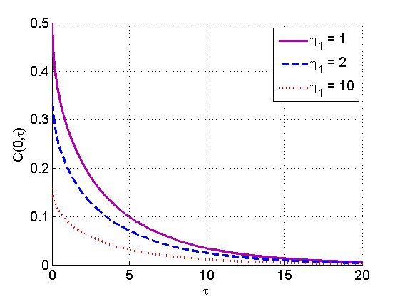
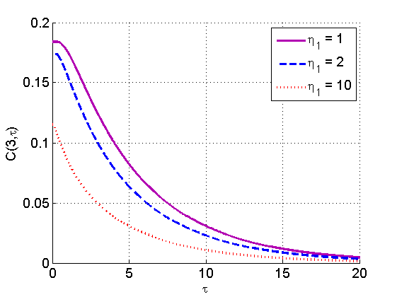
Figure 3: Space-time covariances for $d=1,\eta_{0}=1,\xi=3,\tilde{D}=1$. (a): Covariances for zero space lag and different ${\eta_{1}}$ are shown. (b): Covariances for $r=3$ and different ${\eta_{1}}$.

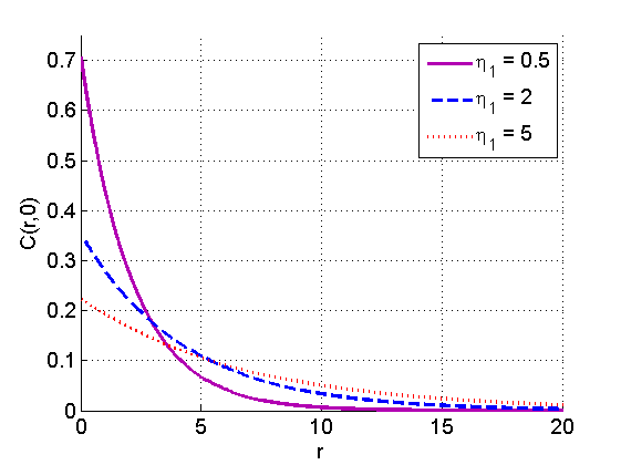
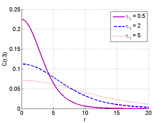
Figure 4: Space-time covariances for $d=1,\eta_{0}=1,\xi=3,\tilde{D}=1$. (a) Spatial dependence at $\tau=0$. (b) Spatial dependence at $\tau=3$.

For $d=1,3$, $\mu=0$ it follows from (31) that the corresponding covariances are given by the equations

$$C({\bf r},\tau)= \frac{\mathrm{e}^{-\tilde{D}\,|\tau|\,}\eta_{0}}{\pi\,{\eta_{1}}\,\xi}\,\int_{0}^{\infty}dk\,\frac{\cos(kr)}{\frac{1}{{\eta_{1}}\,\xi^{2}}+k^{2}}\,\mathrm{e}^{-\tilde{D}\,|\tau|\,\left(\eta_{1}k^{2}\xi^{2}\right)}$$ (62)

and

$$C({\bf r},\tau)= \frac{\mathrm{e}^{-\tilde{D}\,|\tau|\,}\eta_{0}\xi}{2\pi^{2}{\eta_{1}}\,r}\,\int_{0}^{\infty}dk\,\frac{k\,\sin(kr)}{\frac{1}{{\eta_{1}}\,\xi^{2}}+k^{2}}\,\mathrm{e}^{-\tilde{D}\,|\tau|\,\left(\eta_{1}k^{2}\xi^{2}\right)}.$$ (63)

The above integrals can be evaluated analytically for ${\eta_{1}}>0$. Applying the identities [ Eq.(1.4.15), p.15] [41] and [ Eq.(2.4.26) p.74] [41], the following explicit formulas are derived for the one- and three-dimensional covariances

$$C({\bf r};\tau) =\frac{\eta_{0}}{4\sqrt{{\eta_{1}}}}\,\left[\mathrm{e}^{-\frac{r}{\sqrt{{\eta_{1}}}\xi}}\operatorname{Erfc}\left(\sqrt{\tilde{D}\,|\tau|}-\frac{r}{2\sqrt{\tilde{D}{\eta_{1}}\,|\tau|\,}\xi}\right)\right.$$ (64)

$$\left.\quad\quad\quad\quad+\,\mathrm{e}^{\frac{r}{\sqrt{{\eta_{1}}}\xi}}\operatorname{Erfc}\left(\sqrt{\tilde{D}\,|\tau|}+\frac{r}{2\sqrt{\tilde{D}{\eta_{1}}\,|\tau|\,}\xi}\right)\right],$$

and

$$C({\bf r};\tau) =\frac{\eta_{0}\xi}{8\pi{\eta_{1}}\,r}\,\left[\mathrm{e}^{-\frac{r}{\sqrt{{\eta_{1}}}\xi}}\operatorname{Erfc}\left(\sqrt{\tilde{D}\,|\tau|}-\frac{r}{2\sqrt{\tilde{D}{\eta_{1}}\,|\tau|\,}\xi}\right)\right.$$ (65)

$$\left.\quad\quad\quad\quad-\mathrm{e}^{\frac{r}{\sqrt{{\eta_{1}}}\xi}}\,\operatorname{Erfc}\left(\sqrt{\tilde{D}\,|\tau|}+\frac{r}{2\sqrt{\tilde{D}{\eta_{1}}\,|\tau|\,}\xi}\right)\right].$$

The covariance function (64) is equivalent to a model derived by Heine starting from the general form of a second-order stochastic partial differential equation [21, 33]. Our result, however, is expressed in terms of the parameters $\eta_{0},{\eta_{1}},\xi,\tilde{D}$ that can be easily identified with properties of the STRF and include the SSRF parameters of spatial random fields. In particular, $\eta_{0}$ is an overall scale coefficient that determines the amplitude of the fluctuations and has units $[X]^{2}$, ${\eta_{1}}$ is a dimensionless rigidity coefficient that suppresses large gradients, $\xi$ is a characteristic length, and $\tilde{D}$ is a characteristic inverse time. We also derive the covariance function (65) which is valid in three spatial dimensions. Note that the presence of ${\eta_{1}}$ in addition to $\xi$ implies that the correlation length is a function of both parameters [30]. In both $d=1$ and $d=3$ for ${\bf r}\rightarrow 0$ and $\tau\rightarrow 0$, the purely temporal and purely spatial covariance models, respectively (59) and (61), are recovered from (64) and (65). In agreement with the zero-lag analysis, the singularity at $r=0$ and $\tau=0$ is present for $d=3$ in (65). This singularity, which denotes that the STRF has infinite variance, is known in Gaussian field theory as well as in statistical modelling [33]. We discuss a remedy for this problem in the next section.

In Figure 2 we plot the covariance functions (64) and (65) for $d=1$ and $d=3$, respectively. For $d=3$ the minimum lags used are equal to $0.1$ to avoid the zero-lag singularity. Figures 3 and 4 demonstrate the dependence of the covariance function (64) in $d=1$ versus the spatial (time) lag under constant time (space) lag for different values of the rigidity coefficient ${\eta_{1}}$. Note that at the larger lag distances, $r=3$ and $\tau=3$ the covariance function is smooth at the origin, i.e., for $\tau=0$ and $r=0$, respectively, in contrast with the non-differentiable peak at $(r=0,\tau=0)$.

7.2 Small-$\mu$ approximation

In the following we assume that $\mu\ll 1$, so that the curvature term in (47) is present but multiplied with a small coefficient. This small perturbation, however, is sufficient to tame the singularity at the origin (zero lag) of the covariance function, effectively by reducing the impact of large-frequency fluctuations.

We use the spectral representation (47) for the covariance function. The exponential $\mathrm{e}^{-A(\kappa,k)}$ in this case is expressed as follows

$$\mathrm{e}^{-A(\kappa,k)}=\mathrm{e}^{-\kappa\beta_{0}-u^{2}\,k^{2}-\mu\,v\,k^{4}},$$

where the coefficients $v$ and $u^{2}$ are defined by means of the following relations and the constant coefficients given by (54b)

$$v=\xi^{4}\left(\tilde{D}|\tau|+\kappa\beta_{0}\right),\;u^{2}=\eta_{1}\xi^{2}\,\left(\tilde{D}\,|\tau|+\kappa\beta_{0}\right).$$ (66)

The exponential component $\exp(-\mu\,v\,k^{4})$ can be approximated using the Taylor expansion truncated at an even order $2M$ as follows

$$\exp\left(-\mu\,v\,k^{4}\right)\approx\sum_{m=0}^{2M}\frac{(-1)^{m}\,\left(\mu\,v\,k^{4}\right)^{m}}{m!}.$$

The even truncation order ensure that the approximation is non-negative. The divergence of the expansion for large $k$ is controlled by the exponential $\exp(-u\,k^{2})$ for ${\eta_{1}}>0$. Therefore, the truncated spectral density corresponds to a permissible covariance function. The resulting expansion of the covariance function (47) is given by the following series of integrals

$$C({\bf r},\tau)\approx \frac{r^{1-d/2}\,\,\mathrm{e}^{-\tilde{D}\,|\tau|\,}}{(2\pi)^{d/2}}\,\sum_{m=0}^{2M}\frac{(-\mu)^{m}}{m!}\,\int_{0}^{\infty}d\kappa\,v^{m}\,Q_{m}(\kappa),$$ (67)

$$Q_{m}(\kappa) =\mathrm{e}^{-\kappa\beta_{0}}\int_{0}^{\infty}dk\,k^{d/2+4m}\,J_{d/2-1}(kr)\,\mathrm{e}^{-u^{2}\,k^{2}}.$$ (68)

The integral over $k$ in $Q_{m}(\kappa)$ can be evaluated using (51) which leads to

$$Q_{m}(\kappa)=\frac{\mathrm{e}^{-\kappa\beta_{0}}}{u^{4m+d}}\,\left(\frac{r}{2}\right)^{d/2-1}\,\frac{\Gamma(d/2+2m)}{\Gamma(d/2)}\,{}_{1}F_{1}\left(2m+\frac{d}{2},\frac{d}{2};\frac{-r^{2}}{4\,u^{2}}\right).$$ (69)

Based on the two equations above, the space-time covariance function becomes

$$C({\bf r},\tau)\approx \frac{2\,\mathrm{e}^{-\tilde{D}\,|\tau|\,}}{(4\pi)^{d/2}}\,\sum_{m=0}^{2M}\frac{(-\mu)^{m}}{m!}\,\frac{\Gamma(d/2+2m)}{\Gamma(d/2)}\,R_{m}(r,\tau),$$ (70)

$$R_{m}(r,\tau)= \int_{0}^{\infty}d\kappa\,\frac{\mathrm{e}^{-\kappa\beta_{0}}\,v^{m}}{u^{4m+d}}\,{}_{1}F_{1}\left(2m+\frac{d}{2},\frac{d}{2};\frac{-r^{2}}{4\,u^{2}}\right).$$ (71)

In the above, the coefficients $v$ and $u^{2}$ are defined in (66), whereas the coefficients $\beta_{0},\beta_{1},\beta_{2}$ are defined in (54b).

7.3 Numerical solutions for general values of $\mu$ and ${\eta_{1}}$

The presence of the parameter $\mu$ in the general space-time model (31) eliminates the observed singularities at the origin for $\mu=0$ . For $\mu>0$ and negative values of the rigidity coefficient ${\eta_{1}}$, i.e. for $-2<{\eta_{1}}<0$ the covariance function develops oscillations.

Based on (31), the space-time covariances for $\mu\neq 0$ in $d=1,3$ are given by the following one dimensional integrals

$$C({\bf r},\tau)= \frac{\mathrm{e}^{-\tilde{D}\,|\tau|}\eta_{0}\xi}{\pi}\,\int_{0}^{\infty}dk\,\frac{\cos(kr)}{1+{\eta_{1}}\,k^{2}\xi^{2}+\mu\,k^{4}\xi^{4}}\,\mathrm{e}^{-\tilde{D}\,|\tau|\,\left(\eta_{1}k^{2}\xi^{2}+\mu\,k^{4}\xi^{4}\right)},$$ (72)

$$C({\bf r},\tau)= \frac{\mathrm{e}^{-\tilde{D}\,|\tau|}\eta_{0}\xi^{3}}{2\pi^{2}{\eta_{1}}}\,\int_{0}^{\infty}dk\,\frac{k^{2}\,\operatorname{sinc}(kr)}{1+{\eta_{1}}\,k^{2}\xi^{2}+\mu\,k^{4}\xi^{4}}\,\mathrm{e}^{-\tilde{D}\,|\tau|\,\left(\eta_{1}k^{2}\xi^{2}+\mu\,k^{4}\xi^{4}\right)}.$$ (73)

The above integrals were evaluated in Mathematica using the NIntegrate function with high working precision. The spectral integrals were truncated using a finite spectral cutoff, i.e. ${\rm k_{c}}=100$. In Figures 5 and 6 we plot the spatial dependence of the covariance functions (72) and (73) for $d=1$ and $d=3$, respectively. Plots correspond to different values of $\mu$ and two different time lags. In all cases, the correlation length drops with increasing $\mu$. Moreover, it is evident in Fig 6 that in the $d=3$ model has finite values at the origin for $\mu>0$.

Figure 7 displays how the covariance function (64) varies in $d=1$ with $r$ for constant $\tau$ and three negative, values of ${\eta_{1}}$. In all cases, the covariances obtained exhibit oscillations; such functions find applications in hydrology and in wave phenomena [27]. In $d=3$ for negative values of ${\eta_{1}}$ oscillating covariances are obtained by (73); in this case, however, the negative hole of the oscillations is reduced.

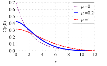
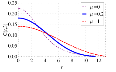
Figure 5: Space-time covariances for $d=1,\eta_{0}=1,{\eta_{1}}=0.5,\xi=3,\tilde{D}=1$. (a) Spatial dependence at $\tau=0$. (b) Spatial dependence at $\tau=3$.

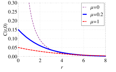
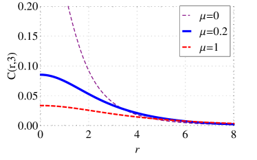
Figure 6: Space-time covariances for $d=3,{\eta_{1}}=0.5,\eta_{0}=1,\xi=3,\tilde{D}=1$. (a) Spatial dependence at $\tau=0$. (b) Spatial dependence at $\tau=3$.

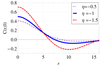
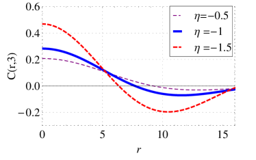
Figure 7: Oscillating space-time covariances for $d=1,\mu=1,\xi=3,\tilde{D}=1$. (a) Spatial dependence at $\tau=0$. (b) Spatial dependence at $\tau=3$.

8 Conclusions

The analysis of spatiotemporal data and statistical mechanics have followed to a large extent separate paths, in spite of the conceptual overlaps between the two fields. The connection between statistical mechanics and geostatistics has been investigated in a series of papers [25, 26, 24, 28, 29, 27]. Herein we demonstrate that space-time covariance functions for the analysis of spatiotemporal data sets can be obtained using ideas from statistical mechanics, such as field theory, maximum entropy, and linear response theory.

We show that a Gaussian field model with an energy functional to which a curvature term is added can be derived from the principle of maximum entropy using suitable data-based constraints. The spatial covariance functions obtained from this energy functional incorporate “interactions” between the sample locations, and they offer increased flexibility due to a richer parametric structure [28, 30]. The “equilibrium” spatial model is herein extended to the space-time domain by means of the covariance equation of motion or the associated Langevin equation for the realizations, both of which are obtained within the framework of the relaxation approximation in linear response theory. The covariance equation of motion provides explicit formulas for the temporal evolution of the spectral density. It is also shown that the associated covariance functions in real space involve integrals that can be analytically computed in different approximation regimes. The obtained solutions provide new types of non-separable, space-time correlation functions without using simplifying but unrealistic assumptions. In contrast with purely statistical models, the STRF model parameters introduced in this paper correspond to distinct properties of the random field.

For future investigations, flexible representations such as the Karhunen-Loève expansion can be used in combination with the Langevin equations to obtain compact expressions for space-time covariance models. The general formulation for construction of space-time covariances based on concepts of statistical mechanics can be extended to incorporate more general models described by non-linear generalized Langevin equations and colored or non-Gaussian driving noises [3, 49].

References

- [1] In E. Porcu, J. Montero, and M. Schlather, editors, Advances and Challenges in Space-time Modelling of Natural Events, Lecture Notes in Statistics. Springer Berlin Heidelberg, 2012.
- [2] M. Abramowitz and I. A. Stegun. Handbook of Mathematical Functions with Formulas, Graphs, and Mathematical Tables. Dover, New York, 9th Dover printing edition, 1964.
- [3] G. A. Athanassoulis, I. C. Tsantili, and Z. G. Kapelonis. Two-time, response-excitation moment equations for a cubic half-oscillator under gaussian and cubic-gaussian colored excitation. Part 1: The monostable case. arXiv preprint arXiv:1304.2195, 2013.
- [4] S. Bochner. Lectures on Fourier Integrals. Princeton University Press, Princeton, NJ, 1959.
- [5] G. Christakos. Random Field Models in Earth Sciences. Academic Press, San Diego, 1992.
- [6] N. Cressie. Spatial Statistics. John Wiley and Sons, New York, 1993.
- [7] N. Cressie and C. L. Wikle. Statistics for Spatio-temporal Data. John Wiley and Sons, New York, 2011.
- [8] S. De Iaco, D. Myers, and D. Posa. Nonseparable space-time covariance models: some parameteric families. Mathematical Geology, 34(1):23–42, 2002.
- [9] S. De Iaco, D. Posa, and D. Myers. Characteristics of some classes of space–time covariance functions. Journal of Statistical Planning and Inference, 143(11):2002 – 2015, 2013.
- [10] S. N. Elogne, D. Hristopulos, and E. Varouchakis. An application of Spartan spatial random fields in environmental mapping: focus on automatic mapping capabilities. Serra, 22(5):633–646, 2008.
- [11] S. N. Elogne and D. T. Hristopulos. Geostatistical applications of Spartan spatial random fields. In A. Soares, M. J. Pereira, and R. Dimitrakopoulos, editors, geoENV VI Geostatistics for Environmental Applications, volume 15 of Quantitative Geology and Geostatistics, pages 477–488. Springer, Berlin, Gemany, 2008.
- [12] C. L. Farmer. Bayesian field theory applied to scattered data interpolation and inverse problems. In A. Iske and J. Levesley, editors, Algorithms for Approximation, pages 147–166. Springer-Verlag, Heidelberg, 2007.
- [13] R. P. Feynman and A. R. Hibbs. Quantum Mechanics and Path Integrals. McGraw-Hill, New York, 1965.
- [14] D. Forster. Hydrodynamic Fluctuations, Broken Symmetry, and Correlation Functions. Addison-Wesley, Redwood City, Calif., 1990.
- [15] M. Fuentes, L. Chen, J. M. Davis, and G. M. Lackmann. Modeling and predicting complex space time structures and patterns of coastal wind fields. Environmetrics, 16(5):449–464, 2005.
- [16] K. Furutsu. On the statistical theory of electromagnetic waves in a fluctuating medium. Journal of Research of the National Institute of Standards and Technology, 67D(3):303–323, 1963.
- [17] I. M. Gel’fand and A. M. Yaglom. Integration in functional spaces and its applications in quantum physics. Journal of Mathematical Physics, 1(1):48–69, 1960.
- [18] N. Goldenfeld. Lectures on Phase Transitions and the Renormalization Group. Frontiers in Physics, 85. Addison-Wesley, 1992.
- [19] I. S. Gradshteyn and I. M. Ryzhik. Tables of Integrals, Series, and Products. Academic Press, New York, 5th edition, 1994.
- [20] P. Guttorp and T. Gneiting. Studies in the history of probability and statistics xlix on the matern correlation family. Biometrika, 93(4):989–995, 2006.
- [21] V. Heine. Models for two-dimensional stationary stochastic processes. Biometrika, 42(1-2):170–178, 1955.
- [22] M. D. Hoffman, D. M. Blei, C. Wang, and J. Paisley. Stochastic variational inference. The Journal of Machine Learning Research, 14(1):1303–1347, 2013.
- [23] P. C. Hohenberg and B. I. Halperin. Theory of dynamic critical phenomena. Review of Modern Physics, 49:435–479, 1977.
- [24] D. Hristopulos and S. Elogne. Analytic properties and covariance functions of a new class of generalized Gibbs random fields. IEEE Transactions on Information Theory, 53(12):4667–4679, 2007.
- [25] D. T. Hristopulos. Spartan Gibbs random field models for geostatistical applications. SIAM Journal of Scientific Computing, 24(6):2125–2162, 2003.
- [26] D. T. Hristopulos. Spatial random field models inspired from statistical physics with applications in the geosciences. Physica A: Statistical Mechanics and its Applications, 365(1):211–216, 2006.
- [27] D. T. Hristopulos. Covariance functions motivated by spatial random field models with local interactions. Stochastic Environmental Research and Risk Assessment, 29:739––754, 2015.
- [28] D. T. Hristopulos and S. N. Elogne. Computationally efficient spatial interpolators based on Spartan spatial random fields. IEEE Transactions on Signal Processing, 57(9):3475–3487, 2009.
- [29] D. T. Hristopulos and E. Porcu. Multivariate spartan spatial random field models. Probabilistic Engineering Mechanics, 37:84–92, 2014.
- [30] D. T. Hristopulos and M. Žukovič. Relationships between correlation lengths and integral scales for covariance models with more than two parameters. Stochastic Environmental Research and Risk Assessment, 25(1):11–19, 2011.
- [31] C. Itzykson and J.-M. Drouffe. Statistical field theory, volume 1. Cambridge University press, New York, 1989.
- [32] E. T. Jaynes. Information theory and statistical mechanics. Physical review, 106(4):620–630, 1957.
- [33] R. H. Jones and Y. Zhang. Models for continuous stationary space-time processes. In Modelling longitudinal and spatially correlated data, pages 289–298. Springer, 1997.
- [34] E. Kalnay. Atmospheric modeling, data assimilation, and predictability. Cambridge, Cambridge, 2003.
- [35] M. Kardar. Statistical Physics of Fields. Cambridge University Press, 2007.
- [36] A. Kolovos, G. Christakos, D. Hristopulos, and M. L. Serre. Methods for generating non-separable spatiotemporal covariance models with potential environmental applications. Advances in Water Resources, 27(8):815–830, 2004.
- [37] J. C. Lemm. Bayesian Field Theory. Johns Hopkins University Press, Baltimore, 2005.
- [38] S. C. Lim and L. P. Teo. Generalized Whittle Matérn random field as a model of correlated fluctuations. Journal of Physics A: Mathematical and Theoretical, 42:105202, 2009.
- [39] C. Ma. Linear combinations of space-time covariance functions and variograms. IEEE Transactions on Signal Processing, 53(3):857–864, 2005.
- [40] C. Ma. Recent developments on the construction of spatio-temporal covariance models. Stochastic Environmental Research and Risk Assessment, 22(1):S39–S47, 2008.
- [41] W. Magnus, H. Bateman, A. Erdélyi, F. Oberhettinger, and F. Tricomi. Tables of integral transforms. McGraw-Hill, 1954.
- [42] U. M. B. Marconi, A. Puglisi, L. Rondonic, and A. Vulpiani. Fluctuation dissipation: Response theory in statistical physics. Physics Reports, 461(4):111–195, 2008.
- [43] G. Mussardo. Statistical field theory. Oxford Univ. Press, 2010.
- [44] E. A. Novikov. Functionals and the random-force method in turbulence theory. Sov. Phys. JETP, 20(5):1290– 1294, 1965.
- [45] C. E. Rasmussen and C. K. I. Williams. Gaussian Processes for Machine Learning. MIT Press, Massachusetts Institute of Technology, 2006.
- [46] M. L. Stein. Space–time covariance functions. Journal of the American Statistical Association, 100(469):310–321, 2005.
- [47] J. Swift and P. C. Hohenberg. Hydrodynamic fluctuations at the convective instability. Physical Review A, 15(1):319, 1977.
- [48] A. Tarantola. Inverse problem theory and methods for model parameter estimation. SIAM, Philadelphia, 2005.
- [49] I. S. C. Tsantili. Two-time response excitation theory for non-linear stochastic dynamical systems. PhD thesis, National Technical University of Athens, 2013.
- [50] M. Žukovič and D. T. Hristopulos. Environmental time series interpolation based on Spartan random processes. Atmospheric Environment, 42(33):7669–7678, 2008.
- [51] M. Žukovič and D. T. Hristopulos. The method of normalized correlations: A fast parameter estimation method for random processes and isotropic random fields that focuses on short-range dependence. Technometrics, 51(2):173–185, 2009.
- [52] H. Wackernagel. Multivariate Geostatistics. Springer Verlag, Berlin, 3rd edition, 2003.
- [53] P. Whittle. On stationary processes in the plane. Biometrika, 41(3/4):434– 449, 1954.
- [54] Q. Xu. Representations of inverse covariances by differential operators. Advances in Atmospheric Sciences, 22(2):181–198, 2005.
- [55] A. M. Yaglom. Correlation Theory of Stationary and Related Random Functions I. Springer Verlag, New York, 1987.
- [56] M. Yaremchuk and A. Sentchev. Multi-scale correlation functions associated with polynomials of the diffusion operator. Quarterly Journal of the Royal Meteorological Society, 138(668):1948–1953, 2012.
- [57] M. Yaremchuk and A. Sentchev. Multi-scale correlation functions associated with polynomials of the diffusion operator. Quarterly Journal of the Royal Meteorological Society, 138(668):1948–1953, 2012.
- [58] M. Yaremchuk and S. Smith. On the correlation functions associated with polynomials of the diffusion operator. Quarterly Journal of the Royal Meteorological Society, 137(660):1927–1932, 2011.
- [59] J. Zinn-Justin. Quantum Field Theory and Critical Phenomena. Oxford Univ. Press, Oxford, 4th edition, 2004.