CEoptim: Cross-Entropy R Package for Optimization

Tim Benham, Qibin Duan, Dirk P. Kroese, Benoît Liquet, CEoptim: Cross-Entropy R Package for Optimization CEoptim: Cross-Entropy R package for Optimization The cross-entropy (CE) method is simple and versatile technique for optimization, based on Kullback-Leibler (or cross-entropy) minimization. The method can be applied to a wide range of optimization tasks, including continuous, discrete, mixed and constrained optimization problems. The new package CEoptim provides the R implementation of the CE method for optimization. We describe the general CE methodology for optimization and well as some useful modifications. The usage and efficacy of CEoptim is demonstrated through a variety of optimization examples, including model fitting, combinatorial optimization, and maximum likelihood estimation. Constrained optimization, continuous optimization, cross-entropy, discrete optimization, Kullback-Leibler divergence, lasso, maximum likelihood, R, regression Cross Entropy, Optimization, R School of Mathemathics and Physics
The University of Queensland
Brisbane, Australia
E-mails:


(corresponding author)

1 Introduction

The cross-entropy (CE) method originates from an adaptive variance minimization algorithm in rubinstein1997 for the estimation rare event probabilities in stochastic networks. It was realized in rubinstein1999 that many optimization problems could be converted into a rare-event estimation problems, providing a rare-event based approach to optimization, where a sequence of probability densities is generated that converges to a degenerate density that concentrates its mass close to the optimizer.

Generally, the CE method involves two iterative phases:

1. Generation of a set of random samples (vectors, trajectories, etc.) according to a specified parameterized model.

2. Updating of the model parameters, based on the best samples generated in the previous step. This is done by Kullback–Leibler (also called cross-entropy) minimization.

Since the appearance of the CE monograph (cebook) and the tutorial (cetutorial2005), the CE method has continued to develop and has been successfully applied to a great variety of difficult optimization problems, including motion planning in robotic systems (kobilarov2012motionplanning), electricity network generation, (kothari09integerprograming), control of infectious diseases (sani2008controlling), buffer allocation (alon2005allocation), Laguerre tessellation (duan2014inverting), and network reliability (kroese2007network). An extensive list of recent work can be found in (ceoptbotev2013). Websites that provide $\mathrm{M}\mathrm{{\scriptstyle ATLAB}}$ code include www.cemethod.org and www.montecarlohandbook.org. Since R has become an essential tool for statistical computation, it is useful to provide an accessible implementation of the CE method for R users, similar to R packages for simulated annealing (xiang2013sa), evolutionary methods (mullendeoptimJss), and particle swarm optimization methods (bendtsenpso).

Some advantages of the CE method are:

• The CE method is a global optimization method which is particularly useful when the objective function has many local optima.

• The CE method can be used to solve continuous, discrete, and mixed optimization problems, which may also include constraints.

• The CE code is extremely compact and is readily written in native R, making further development and modifications easy to implement.

• The CE method is based on rigorous mathematical and statistical principles.

Our aim is not to replace the standard optimization solvers such as optim and nlm but to provide a viable alternative in cases where standard gradient or simplex-based solvers are not applicable (e.g., when the optimization problem contains both discrete and continuous variables) or are expected to do poorly (e.g., when there are many local optima).

The rest of this paper is organized as follows. In Section 2, we sketch the general theory behind the CE method, which leads to the basic CE algorithm. In Section 3, we describe a variety of optimization scenarios, including continuous, discrete and constrained mixed problems, to which CE can be applied effectively. The description and usage of the CEoptim package are given in Section 4. Section 5 demonstrates the capability of the package through a range of numerical examples. In the final section we make concluding remarks for CEoptim.

2 CE method for optimization

Let $\mathscr{X}$ be an arbitrary set of states and let $S$ be a real-valued performance function on $\mathscr{X}$. Suppose the goal is to find the minimum of $S$ over $\mathscr{X}$, and the corresponding minimizer $\mathbf{x}^{*}$ (assuming, for simplicity, that there is only one). Denote the minimum by $\gamma^{*}$, so that

$$S(\mathbf{x}^{*})=\gamma^{*}=\min_{\mathbf{x}\in\mathscr{X}}S(\mathbf{x}).$$ (1)

The CE methodology for optimization is adapted from the CE methodology for rare event estimation in the following way. Associate with the above problem (1) the estimation of the probability $\ell=\mathbb{P}(S(\mathbf{X})\leqslant\gamma)$, where $\mathbf{X}$ has some probability density $f(\mathbf{x};\mathbf{u})$ on $\mathscr{X}$ (for example corresponding to the uniform distribution on $\mathscr{X}$) depending on a parameter $\mathbf{u}$ and a level $\gamma$. Thus, for optimization problems randomness is purposely introduced in order to make the model stochastic. If $\gamma$ is chosen close to the unknown $\gamma^{*}$, then $\ell$ is typically a rare-event probability. One of the most effective ways to estimate rare-event probabilities is to use importance sampling. In particular, to estimate $\ell=\mathbb{P}(S(\mathbf{X})\leqslant\gamma)$ one can use the importance sampling estimator

$$\widehat{\ell}=\frac{1}{N}\sum_{i=1}^{N}\frac{f(\mathbf{X}_{i})}{g(\mathbf{X}_{i})}\mathrm{I}\{S(\mathbf{X}_{i})\leqslant\gamma\},$$

where $\mathbf{X}_{1},\ldots,\mathbf{X}_{N}$ are iid samples from a well-chosen importance sampling density $g$. The optimal importance sampling density is in this case $g^{*}(\mathbf{x})=f(\mathbf{x})\mathrm{I}\{S(\mathbf{x})\leqslant\gamma\}/\ell$, which gives a zero-variance estimator, but depends on the unknown quantity $\ell$. The main idea behind the CE method for estimation is to adaptively determine an importance sampling pdf $f(\mathbf{x};\mathbf{v}^{*})$ — hence within the same family as the original distribution — that is close to $g^{*}$ in Kullback–Leibler sense. Specifically, a parameter $\mathbf{v}^{*}$ is sought that minimizes the cross-entropy distance

$${\mathcal{D}}(g^{*},f(\cdot;\mathbf{v}))=\mathbb{E}_{g^{*}}\left[\ln\frac{g^{*}(\mathbf{X})}{f(\mathbf{X};\mathbf{v})}\right]=\int g^{*}(\mathbf{x})\ln g^{*}(\mathbf{x})\,\mathrm{d}\mathbf{x}-\int g^{*}(\mathbf{x})\ln f(\mathbf{x};\mathbf{v})\,\mathrm{d}\mathbf{x}\;.$$

This is equivalent to maximizing, with respect to $\mathbf{v}$,

$$\int f(\mathbf{x};\mathbf{u})\mathrm{I}\{S(\mathbf{x})\leqslant\gamma\}\ln f(\mathbf{x};\mathbf{v})\,\mathrm{d}\mathbf{x}=\mathbb{E}_{\mathbf{u}}\left[\mathrm{I}\{S(\mathbf{X})\leqslant\gamma\}\ln f(\mathbf{X};\mathbf{v})\right]\;,$$

which in turn can be estimated by maximizing the sample average

$$\frac{1}{N}\sum_{i=1}^{N}\left[\mathrm{I}\{S(\mathbf{X}_{i})\leqslant\gamma\}\ln f(\mathbf{X}_{i};\mathbf{v})\right]\;,$$ (2)

where $\mathbf{X}_{1},\ldots,\mathbf{X}_{N}$ is an iid sample from $f(\mathbf{x};\mathbf{u})$. This is, in essence, maximum likelihood estimation. In particular, (2) gives the maximum likelihood estimator of $\mathbf{v}$ based on only the samples $\mathbf{X}_{1},\ldots,\mathbf{X}_{N}$ that have a function value less than or equal to $\gamma$. These are the so-called elite samples.

The relevance to optimization is that when $\gamma$ is close to the (usually unknown) minimum $\gamma^{*}$, then the importance sampling density $g^{*}$ concentrates most of its mass in the vicinity of the minimizer $\mathbf{x}^{*}$. Sampling from such a distribution thus produces optimal or near-optimal states. The CE method for optimization produces a sequence of levels $({\gamma}_{t})$ and reference parameters $({\mathbf{v}}_{t})$ determined from (2) such that the former tends to the optimal $\gamma^{*}$ and the latter to the optimal reference vector $\mathbf{v}^{*}$, where $f(\mathbf{x};\mathbf{v}^{*})$ corresponds to the point mass at $\mathbf{x}^{*}$; see, e.g., (mcbook, Page 251).

The generic steps for CE optimization are specified in Algorithm 1.

Algorithm 1 Generic CE algorithm

0:  Initial parameter vector $\mathbf{v}_{0}$. Sample size $N$. Rarity parameter $\varrho$.

0:  Sequence of levels $({\gamma}_{t})_{t=1}^{T}$ and parameters $({\mathbf{v}}_{t})_{t=1}^{T}$.

1:  Let $N^{\mathop{\rm e}}=\left\lceil\varrho N\right\rceil$ (number of elite samples) and set $t=1$ (level counter).

2:  while the sampling distribution is not degenerate do

3:     Generate $\mathbf{X}_{1},\ldots,\mathbf{X}_{N}{\>{\sim}_{\mathrm{iid}}\>}f(\cdot;{\mathbf{v}}_{t-1})$. Calculate the performances $S(\mathbf{X}_{i})$ for all $i$, and order them from smallest to largest: $S_{(1)}\leqslant\ldots\leqslant S_{(N)}$. Let ${\gamma}_{t}$ be the sample $\varrho$-quantile of performances; that is, ${\gamma}_{t}=S_{(N^{\mathop{\rm e}})}$.

4:     Use the same sample $\mathbf{X}_{1},\ldots,\mathbf{X}_{N}$ and solve the stochastic program

$$\max_{\mathbf{v}}\sum_{k=1}^{N}\mathrm{I}\{S(\mathbf{X}_{k})\leqslant{\gamma}_{t}\}\,\ln f(\mathbf{X}_{k};\mathbf{v})\;.$$ (3)

Denote the solution by ${\mathbf{v}}_{t}$. Increase $t$ by 1.

5:  end while

To run the algorithm, one needs to provide the class of sampling densities $\{f(\cdot;\mathbf{v})\}$, the initial vector ${\mathbf{v}}_{0}$, the sample size $N$, the rarity parameter $\varrho$, and the stopping criterion. It is prudent to keep track of the overall best function value and corresponding state, and report these at the end of the algorithm as the optimal value and optimizer, respectively. The progression of level parameter ${\gamma}_{t}$ gives an indication how well the algorithm converges.

As (3) is simply a maximum likelihood estimation step involving only the elite samples, it is possible to derive easy parameter updates for standard sampling distributions. The following two special cases are of particular importance.

1. Multivariate normal distribution. Suppose each $\mathbf{X}$ is sampled from an $n$-dimensional multivariate normal distribution with independent components. The parameter vector $\mathbf{v}$ in the CE algorithm can be taken as the $2n$-dimensional vector of means and standard deviations. In each iteration these means and standard deviations are updated according to the sample mean and sample standard deviation of the elite samples.

2. Multivariate Bernoulli distribution. Suppose each $\mathbf{X}$ is sampled from an $n$-dimensional Bernoulli distribution with independent components. The parameter vector $\mathbf{v}$ in the CE algorithm can be taken as the $n$-dimensional vector of success probabilities. In each iteration the $i$th success probability is updated according to the mean number of successes (1s) at the $i$th position of the elite samples.

Remark 1 (Parameter Smoothing)

Various modifications of the basic CE algorithm have been proposed in recent years. One such is modification is parameter smoothing, where at the $t$th iteration the sampling parameter is updated via

$${\mathbf{v}}_{t}=\alpha\,\widetilde{\mathbf{v}}_{t}+(1-\alpha)\,{\mathbf{v}}_{t-1},$$ (4)

where $\widetilde{\mathbf{v}}_{t}$ is the solution to (3) and $0\leqslant\alpha\leqslant 1$ is a fixed smoothing parameter.

Smoothed updating can prevent the sampling distribution from converging too quickly to a sub-optimal degenerate distribution. This is especially relevant for the multivariate Bernoulli case where, once a success probability reaches 0 or 1, it can no longer change.

It is also possible to use different smoothing parameters for different components of the parameter vector (e.g., the means and the variances).

Remark 2 (Choice of sampling densities)

Although sampling distributions with independent components are the most convenient to use in a CE implementation, it is sometimes advantageous consider more complex sampling models, such as mixture models. In this case the updating of parameters (maximum likelihood estimation) may no longer be trivial, but one can instead employ fast methods such as the EM algorithm to determine the parameter updates.

Remark 3 (Choice of the CE parameters)

The CE method is fairly robust with respect to the choice of the parameters. The rarity parameter $\varrho$ is typically chosen between 0.01 and 0.1. The number of elite samples $N^{\mathop{\rm e}}=\left\lceil\varrho N\right\rceil$ should be large enough to obtain a reliable parameter update in (3). For example, if the dimension of $\mathbf{v}$ is $d$, the number of elites should be in the order of $10\,d$ or higher.

3 Optimization scenarios

In this section we consider a number optimization scenarios to which CEoptim could be applied.

3.1 Continuous optimization

Consider a continuous optimization problem with state space $\mathscr{X}=\mathbb{R}^{n}$. The sampling distribution on $\mathbb{R}^{n}$ can be quite arbitrary and does not need to be related to the objective function $S$. Usually, the random vector $\mathbf{X}=(X_{1},\ldots,X_{n})^{\top}\in\mathbb{R}^{n}$ is generated from a Gaussian distribution with independent components, characterized by a vector $\boldsymbol{\mu}$ of means and a vector $\boldsymbol{\sigma}$ of standard deviations. At each iteration of the CE method, these vectors of parameters are updated as the means and standard deviation of the elite samples. During the course of the algorithm a sequence of $(\boldsymbol{\mu}_{t})$ and $(\boldsymbol{\sigma}_{t})$ are generated, such that $\boldsymbol{\mu}_{t}$ tends to the optimizer $\mathbf{x}^{*}$, while the vector of standard deviations tends to the zero vector. At the end of the algorithm one should obtain a degenerated probability density with mean $\boldsymbol{\mu}_{T}$ approximately equal to the optimizer $\mathbf{x}^{*}$ and all standard deviations close to 0. A possible stopping criterion is to stop when all components in $\boldsymbol{\sigma}_{T}$ are smaller than some $\varepsilon$. This scheme is referred to as normal updating.

CEoptim implements the normal updating scheme for continuous optimization.

3.2 Discrete optimization

If the state space $\mathscr{X}$ is finite, the optimization problem is often referred to as a discrete or combinatorial optimization problem, where $\mathscr{X}$ could be the space of combinatorial objects, such as binary vectors, trees, graphs, etc. To apply the CE method to a discrete optimization problem, one needs a convenient parameterized random mechanism to generate samples.

For discrete optimization CEoptim implements sampling from state spaces $\mathscr{X}$ of the form $\{0,1,\ldots,c_{1}-1\}\times\cdots\times\{0,1,\ldots,c_{n}-1\}$, where the $\{c_{i}\}$ are strictly positive integers. The components of the random vector $\mathbf{X}=(X_{1},\ldots,X_{n})\in\mathscr{X}$ are taken to be independent, so that its distribution is determined by a sequence of probability vectors $\mathbf{p}_{1},\ldots,\mathbf{p}_{n}$, with the $j$th component of $\mathbf{p}_{i}$ corresponding to $p_{ij}=\mathbb{P}(X_{i}=j)$. For a given elite sample set $\mathscr{E}$ of size $N^{\mathop{\rm e}}$, the CE updating formulas for these probabilities are

$${p}_{ij}=\frac{\sum_{\mathbf{X}\in\mathscr{E}}\mathrm{I}\{X_{i}=j\}}{N^{\mathop{\rm e}}},\quad i=1,\ldots,n,\quad j=0,\ldots,c_{n}-1,$$ (5)

where $\mathrm{I}$ denotes the indicator function. Hence, at each iteration, probability $p_{ij}$ is updated simply as the average number of times that the $i$th component of the elite vectors is equal to $j$. A possible stopping rule for a discrete optimization problem is to stop when the overall best objective value does not change over a number of iterations. Alternatively, one could stop when the sampling distribution has degenerated sufficiently; for example, when all $\{p_{ij}\}$ are no further than $\varepsilon$ away from either 0 or 1.

3.3 Constrained optimization

The general optimization problem (1) also covers constrained optimization, where the search space $\mathscr{X}$ could, for example, be defined by a system of inequalities:

$$G_{i}(\mathbf{x})\leqslant 0,\quad i=1,\ldots,k.$$ (6)

One way to deal with constraints is to use acceptance-rejection: generate a random vector $\mathbf{X}$ on a simple search space that contains $\mathscr{X}$, and accept or reject it based on whether the sample falls in $\mathscr{X}$ or not. Alternatively, one could try to sample directly from a truncated distribution on $\mathscr{X}$, e.g., using Gibbs sampling.

CEoptim implements linear constraints for continuous optimization of the form $A\mathbf{x}\leqslant\mathbf{b}$, where $A$ is a matrix and $\mathbf{b}$ a vector. The program will use either acceptance–rejection or Gibbs sampling to sample from the multivariate normal distribution truncated to the constraint set.

A second approach to handle constraints is to introduce a penalty function. For example, for the constraints (6), the objective function could be modified to

$$\widetilde{S}(\mathbf{x})=S(\mathbf{x})+\sum_{i=1}^{k}H_{i}\max\{G_{i}(\mathbf{x}),0\},$$ (7)

where $H_{i}<0$ measures the importance of the $i$th penalty. To use the penalty approach with CEoptim the user simply needs to modify the objective function according to (7). The choice of the penalty constants $\{H_{i}\}$ is problem specific and may need to be determined by trial and error.

4 CEoptim description

In this section we describe how to use CEoptim.

The CEoptim function is the main function of the package CEoptim. It can be used to solve continuous and discrete optimization problems as well as mixtures thereof.

4.1 Usage

CEoptim(f, f.arg=NULL, maximize=FALSE, continuous=NULL, discrete=NULL,
        N=100L, rho=0.1, iterThr=1e4L, noImproveThr= 5, verbose=FALSE)

4.2 Arguments

Argument	Description
f	Function to be optimized. Can have continuous and discrete arguments.
f.arg	List of additional fixed arguments passed to function f.
maximize	Logical value determining whether to maximize or minimize the objective function.
continuous	List of arguments for the continuous optimization part, consisting of:
—  mean	Vector of initial means.
—  sd	Vector of initial standard deviations.
—  smoothMean	Smoothing parameter for the vector of means. Default value 1 (no smoothing).
—  smoothSd	Smoothing parameter for the standard deviations. Default value 1 (no smoothing).
—  sdThr	Positive numeric convergence threshold. Check whether the maximum standard deviation is smaller than sdThr. Default value 0.001.
—  conMat	Coefficient matrix of linear constraint conMat $\mathbf{x}\leqslant$ conVec.
—  conVec	Value vector of linear constraint linear constraint conMat $\mathbf{x}\leqslant$ conVec.
discrete	List of arguments for the discrete optimization part, consisting of:
—  categories	Integer vector which defines the allowed values of the categorical variables. The ith categorical variable takes values in the set $\{0,1,\ldots,\text{\code{categories(i)}}-1\}$.
—  probs	List of initial probabilities for the categorical variables. Defaults to equal (uniform) probabilities.
—  smoothProb	Smoothing parameter for the probabilities of the categorical sampling distribution. Default value 1 (no smoothing).
—  probThr	Positive numeric convergence threshold. Check whether all probabilities in the categorical sampling distributions deviate less than probThr from either 0 or 1. Default value 0.001.
N	Integer representing the CE sample size.
rho	Value between 0 and 1 representing the elite proportion.
iterThr	Termination threshold on the largest number of iterations.
noImproveThr	Termination threshold on the largest number of iterations during which no improvement of the best function value is found.
verbose	Logical value set for CE progress output.

4.3 Value

CEoptim returns a list with the following components.

optimum	Optimal value of f.
optimizer	List of the location of optimal value, consisting of:
—  continuous	Continuous part of the optimizer.
—  discrete	Discrete part of the optimizer.
termination	List of termination information consisting of:
—  niter	Total number of iterations upon termination.
—  convergence	One of the following termination statements: • Not converged, if the number of iterations reaches iterThr; • The optimum did not change for noImproveThr iterations, if the best value has not improved for noImproveThr iterations; • Variances converged, otherwise.
states	List of intermediate results computed at each iteration. It consists of the iteration number (iter), the best overall value (optimum) and the worst value of the elite samples, (gammat). The means (mean) and maximum standard deviation (maxSd) of the elite set are also included for continuous cases, and the maximum deviations (maxProbs) of the sampling probabilities to either $0$ or $1$ are included for discrete cases.
states.probs	List of categorical sampling probabilities computed at each iteration. Will only be returned for discrete and mixed cases.

4.4 Note

• Although partial parameter passing is allowed outside lists, it is recommended that parameters names are specified in full. Parameters inside lists have to specified completely.

• Because CEoptim is a random function it is useful to (1) set the seed for the random number generator (for testing purposes), and (2) investigate the quality of the results by repeating the optimization a number of times.

5 Numerical examples

The following examples illustrate the use, flexibility, and efficacy of the CEoptim function from the package CEoptim.

5.1 Maximizing the peaks function

Suppose we wish to maximize $\mathrm{M}\mathrm{{\scriptstyle ATLAB}}$’s well-known peaks function, given by

$$S(\mathbf{x})=3(1-x_{1})^{2}\,\mathrm{e}^{-x_{1}^{2}-(x_{2}+1)^{2}}-10\left(\frac{x_{1}}{5}-x_{1}^{3}-x_{2}^{5}\right)\mathrm{e}^{-x_{1}^{2}-x_{2}^{2}}-\frac{1}{3}\mathrm{e}^{-(x_{1}+1)^{2}-x_{2}^{2}}\;.$$ (8)

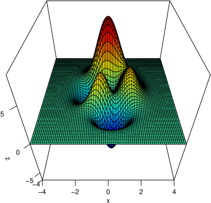
Figure 1: Peaks function

The peaks function has three local maxima and three local minima, with a global maximum at $\mathbf{x}^{*}\approx(-0.0093,1.58)$ of $S(\mathbf{x}^{*})\approx 8.1$, and the other two local maximum are $S(\mathbf{x}_{1})=3.78$ at $(-0.46,-0.63)$ and $S(\mathbf{x}_{2})=3.59$ at $(1.29,-0.0049)$.

To solve the problem with CEoptim, using normal updating, we must specify the vector of initial means $\boldsymbol{\mu}_{0}$ and standard deviations $\boldsymbol{\sigma}_{0}$ of the 2-dimensional Gaussian sampling distribution. The initial sampling distribution should cover, roughly, the region where the maximizer is thought to lie. As an example we take $\boldsymbol{\mu}_{0}=(-3,-3)$ and $\boldsymbol{\sigma}_{0}=(10,10)$. The important point is that the standard deviations are chosen large enough. Since this is a maximization problem, we have to set maximize=T. For the other parameters we take their default values. Note that there are only four parameters to be updated in each iteration, so a sample size of $N=100$ is suitable. R> require(CEoptim) R> fun <- function(x)3*(1-x[1])^2*exp(-x[1]^2 - (x[2]+1)^2)-10*(x[1]/5 + -x[1]^3 - x[2]^5)*exp(-x[1]^2 - x[2]^2) + -1/3*exp(-(x[1]+1)^2 - x[2]^2)

R> set.seed(1234) # for verification purpose only R> mu0 <- c(-3,-3); sigma0 <- c(10,10) R> res <- CEoptim(fun, maximize=T, continuous=list(mean=mu0,sd=sigma0)) R> res

The output of this implementation is as below: Optimizer for continuous part: -0.009390034 1.581405 Optimum: 8.106214 Number of iterations: 7 Convergence: Variance converged

The reader may check that optim applied to the minimization of $-f$ can easily find the wrong optimizer, e.g., when the starting value is $(0,0)$.

5.2 Non-linear regression

We next consider a more complicated optimization task, involving data generated from the well-known FitzHugh–Nagumo differential equations:

$$\begin{split}\frac{\mathrm{d}V_{t}}{\mathrm{d}t}&=c\left(V_{t}-\frac{V_{t}^{3}}{3}+R_{t}\right)\;,\\ \frac{\mathrm{d}R_{t}}{\mathrm{d}t}&=-\frac{1}{c}(V_{t}-a+bR_{t})\;,\end{split}$$ (9)

which model the behavior of certain types of neurons (nagumo62). Ramsay07 consider estimating the parameters $a$, $b$, and $c$ from noisy observations of $(V_{t})$ by using a generalized smoothing approach. The simulated data in Figure 2 (saved as data(FitzHugh)) correspond to the values of $V_{t}$ obtained from (9) at times $0,0.05,\ldots,20.0$, adding Gaussian noise with standard deviation 0.5. That is, we use the non-linear regression model

$$Y_{i}=V_{0.05i}(\mathbf{x})+\varepsilon_{i},\quad i=1,\ldots,400\;,$$ (10)

where the $\{\varepsilon_{i}\}$ are iid with a ${\sf N}(0,\sigma^{2})$ distribution, $V_{0.05i}(\mathbf{x})$ is the solution to (9) for time $t=0.05i$, and $\mathbf{x}=(a,b,c,V_{0},R_{0})$ is the vector of parameters. The true parameter values are here $a=0.2$, $b=0.2$, and $c=3$. The initial conditions are $V_{0}=-1$ and $R_{0}=1$.

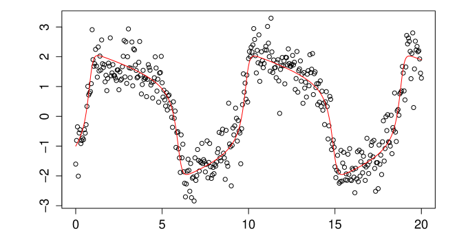
Figure 2: Simulated data (points) and “unknown” true curve (red).

Estimation of the parameters via the CE method can be established by minimizing the least-squares performance

$$S(\mathbf{x})=\sum_{i=0}^{400}\left(y_{i}-V_{0.05i}(\mathbf{x})\right)^{2}\;,$$ (11)

where the $\{y_{i}\}$ are the simulated data from the model (10). Note that we assume that also the initial conditions are unknown.

We use the deSolve package to numerically solve the FitzHugh–Nagumo differential equations (9). Hereto, we first define the function FN.

R> FN <- function(t,state,parameters) with(as.list(c(state,parameters)), dV <- c*(V-V^3/3+R) dR <- -1/c*(V-a+b*R) list(c(dV,dR)) )

The following function ssres now implements the objective function in (11).

R> ssres <- function(x,fundf,times,y) parameters <- c(a=x[1],b=x[2],c=x[3]) state <- c(V=x[4],R=x[5]) out <- ode(y=state,times=times,func=fundf,parms=parameters) return(sum((out[,2]-y)^2)) CEoptim could be used with ${\boldsymbol{\mu}}_{0}=(0,0,5,0,0)$ and ${\boldsymbol{\sigma}}_{0}=(1,1,1,1,1)$. Constant smoothing parameters $\alpha=0.9$ and $\beta=0.5$ were used for the $\{{\boldsymbol{\mu}}_{t}\}$ and the $\{{\boldsymbol{\sigma}}_{t}\}$, respectively. To see the progress of the algorithm we set verbose to TRUE. The other arguments remain default.

R> require(deSolve) R> require(CEoptim) R> set.seed(123405) R> times <- seq(0,20,by=0.05) R> data(FitzHugh)

R> res<- CEoptim(ssres, f.par = list(fundf=FN, times=times, y=ySim), continuous= list(mean=c(0,0,5,0,0), sd=c(1,1,1,1,1), smoothMean=0.9,smoothSd=0.5), verbose=TRUE) The final output is as follows: R> res Optimizer for continuous part: 0.1959748 0.2395983 3.001453 -0.9938222 0.9791585 Optimum: 102.8005 Number of iterations: 41 Convergence: Variance converged The output shows the estimates (notice that the initial condition was assumed to be unknown): ${\widehat{a}}=0.1959748,{\widehat{b}}=0.2395983,{\widehat{c}}=3.0014526,{\widehat{V}}_{0}=-0.9938222$, and ${\widehat{R}}_{0}=0.9791585$, with the maximum likelihood estimate $\widehat{\sigma}=\sqrt{102.8005/400}=0.507$ for the residual standard deviation $\sigma$. The reader may check that fitted curve is practically indistinguishable from the true one in Figure 2.

To illustrate how the sampling distributions change during the CE process, we have plotted in Figure 3 the evolution of the sampling pdf for the first parameter $a$, from the 15th to the final iteration. As can be seen from the figure, the sampling distribution converges to a point distribution around the optimal value for $a$.

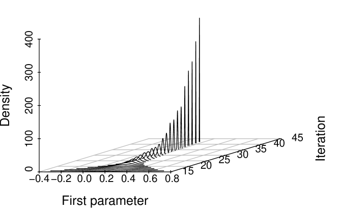
Figure 3: The evolution of the sampling pdf for the first parameter $a$

5.3 Max-cut problem

The max-cut problem in graph theory can be formulated as follows. Given a weighted graph $(V,E)$ with node set $V=\{1,\ldots,n\}$ and edge set $E$, partition the nodes of the graph into two subsets $V_{1}$ and $V_{2}$ such that the sum of the (nonnegative) weights of the edges going from one subset to the other is maximized. Let $C=(C_{ij})$ be the matrix of weights. The objective is to maximize

$$\sum_{(i,j)\in V_{1}\times V_{2}}(C_{ij}+C_{ji})\;$$ (12)

over all cuts $\{V_{1},V_{2}\}$. Such a cut can be conveniently represented by a binary cut vector $\mathbf{x}=(x_{1},x_{2},\ldots,x_{n})$, where $x_{i}=1$ indicates that $i\in V_{1}$. Let $\mathscr{X}$ be the set of cut vectors and let $S(\mathbf{x})$ be the value of the cut represented by $\mathbf{x}$, as given in (12).

To maximize $S$ via the CE method one can generate the random cut vectors by drawing each component (except the first one, which is set to 1) independently from a Bernoulli distribution, that is, $\mathbf{X}=(X_{1},X_{2},\ldots,X_{n})\sim{\sf Ber}(\mathbf{p})$, where $\mathbf{p}=(1,p_{2},\ldots,p_{n})$. In this case the updated success probability for the $i$th component is the mean of the $i$-th components of the vectors in the elite set.

As an example, consider the network from lesmis_knuth describing the coappearances of 77 characters from Victor Hugo’s novel Les Miserables. Each node of the network represents a selected character and edges connect any pair of characters that coappear. The weights of the edges are the number of such coappearances. Using CEoptim, the data can be loaded via the command data(lesmis). The network is displayed in Figure 4, using the graph analysis package sna. R> library(sna) R> library(CEoptim) R> data(lesmis) R> gplot(lesmis,gmode="graph")

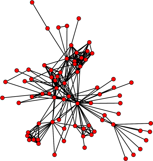
Figure 4: Network of coappearances

For any fixed cost matrix costs and cut vector x, the objective function of the max-cut problem can be written as: R> fmaxcut <- function(x,costs) v1 <- which(x==1) v2 <- which(x==0) return( sum(costs[v1,v2]))

To optimize this function with the CEoptim package, we specify the following arguments: discrete$probs={(0,1); (0.5.0.5);…;(0.5,0.5)}, sample size N=3000 and optimization type: maximize=T. To see the output we set verbose=TRUE. The other arguments are taken as default. Note that users only need to specify either categories or probs, if both of them are specified, then categories will be overridden. R> set.seed(5) R> p0<-list() R> for(i in 1:77)p0<-c(p0,list(rep(0.5,2))) R> p0[[1]] = c(0,1) R> res <- CEoptim(fmaxcut,f.arg=list(costs=lesmis),maximize=T, verbose=TRUE,discrete=list(probs=p0),N=3000L)

R> ind <- res$optimizer$discrete R> group1 <- colnames(lesmis)[which(ind==TRUE)] R> group2 <- colnames(lesmis)[which(ind==FALSE)] The output of CEoptim is as follows: R> res Optimizer for discrete part: 1 0 1 0 0 0 0 0 0 0 1 0 0 1 1 1 0 0 1 1 0 1 0 1 0 1 1 1 1 0 0 1 1 1 1 1 1 0 0 0 0 1 0 1 0 0 1 0 1 1 1 0 1 1 1 0 0 0 0 1 1 0 1 0 0 1 1 1 1 0 0 1 0 1 0 0 0 Optimum: 535 Number of iterations: 20 Convergence: Optimum did not change for 5 iterations Note that character 1 (Myriel) is always in group1. The initial probabilities for the other characters are $0.5$. With states.probs, we can plot the evolution of the probabilities that each character belongs to group1; see Figure LABEL:fig:probsevolution. R> probs <- res$states.probsR>X<-matrix(NA,nrow=length(probs),ncol=77)R>prob0<-cbind(1,t(rep(0.5,76)))R>for(iin1:length(probs))for(jin1:77)X[i,j]<-resstates.probs[[i]][[j]][2]R>X<-rbind(prob0,X)R>par(mfcol=c(5,2),mar=c(1,1.5,1,1.5),oma=c(1,1,1,1))R>for(iin1:5)plot(X[i,],type=\mathrm{"}h\mathrm{"},lwd=4,col=\mathrm{"}blue\mathrm{"},ylim=c(0,1),xaxt=\mathrm{"}n\mathrm{"},yaxt=\mathrm{"}n\mathrm{"},ylab=\mathrm{"}\mathrm{"},main=paste(\mathrm{"}t=\mathrm{"},i-1,sep=\mathrm{"}\mathrm{"}))axis(2,at=0.5,labels=0.5)R>for(iin1:5)plot(X[1+4\ast i,],type=\mathrm{"}h\mathrm{"},lwd=4,col=\mathrm{"}blue\mathrm{"},ylim=c(0,1),xaxt=\mathrm{"}n\mathrm{"},yaxt=\mathrm{"}n\mathrm{"},ylab=\mathrm{"}\mathrm{"},main=paste(\mathrm{"}t=\mathrm{"},1+4\ast i,sep=\mathrm{"}\mathrm{"}))axis(2,at=0.5,labels=0.5)\text{Figure 5Figure 55Figure 55Evolutionofcategoricalsamplingprobabilitie}$