A Study of Multi-frequency Polarization Pulse Profiles of Millisecond Pulsars

Abstract

We present high signal-to-noise ratio, multi-frequency polarization pulse profiles for $24$ millisecond pulsars that are being observed as part of the Parkes Pulsar Timing Array (PPTA) project. The pulsars are observed in three bands, centred close to $730$, $1400$ and $3100$ MHz, using a dual-band 10 cm/50 cm receiver and the central beam of the 20 cm multibeam receiver. Observations spanning approximately six years have been carefully calibrated and summed to produce high S/N profiles. This allows us to study the individual profile components and in particular how they evolve with frequency. We also identify previously undetected profile features. For many pulsars we show that pulsed emission extends across almost the entire pulse profile. The pulse component widths and component separations follow a complex evolution with frequency; in some cases these parameters increase and in other cases they decrease with increasing frequency. The evolution with frequency of the polarization properties of the profile is also non-trivial. We provide evidence that the pre- and post-cursors generally have higher fractional linear polarization than the main pulse. We have obtained the spectral index and rotation measure for each pulsar by fitting across all three observing bands. For the majority of pulsars, the spectra follow a single power-law and the position angles follow a $\lambda^{2}$ relation, as expected. However, clear deviations are seen for some pulsars. We also present phase-resolved measurements of the spectral index, fractional linear polarization and rotation measure. All these properties are shown to vary systematically over the pulse profile.

1 Introduction

Millisecond pulsars (MSPs) are a special subgroup of radio pulsars. Compared with ‘normal’ pulsars, they have shorter spin periods and much smaller spin-down rates, and therefore have larger characteristic ages and weaker implied dipole magnetic fields. The short spin periods and highly stable average pulse shapes of MSPs make them powerful tools to investigate a large variety of astrophysical phenomena. In particular, much recent work has been devoted to a search for a gravitational-wave background using observations of a large sample of MSPs in a “Pulsar Timing Array” (e.g., Foster & Backer, 1990). The Parkes Pulsar Timing Array (PPTA) project (Manchester et al. 2013) regularly observes $24$ MSPs. The PPTA search for gravitational waves has been described in other papers including Shannon et al. (2013), Zhu et al. (2014) and Wang et al. (2015).

We have not yet detected gravitational waves. In order to do so we will need to observe a larger set of pulsars, increase the span of the observations and/or to increase the timing precision achieved for each observation (e.g., Cordes & Shannon, 2012). Determining whether it is possible to improve the timing precision and, if so, by how much relies on our understanding of the stability of pulse profiles (e.g., Shannon et al., 2014) and also on the profile frequency evolution and polarization properties. For our work we study the large number of well calibrated, high signal-to-noise ratio (S/N) multi-frequency polarization pulse profiles that have been obtained as part of the PPTA project.

An earlier analysis of the 20 cm pulse profiles from the PPTA sample was published by Yan et al. (2011a). This earlier work is extended in this paper as: (1) we include four new pulsars that have recently been added to the PPTA sample; (2) we utilise more modern pulsar backend instrumentation than was available to Yan et al. (2011a); (3) we use longer data sets enabling higher S/N profiles; and (4) we provide polarization pulse profiles in three independent bands (at 10, 20 and 50 cm). We note that, even though we have mainly the same sample of pulsars as was described by Yan et al. (2011a), our data sets are independent (i.e., no data is in common between this and the earlier publication).

It has been shown that, compared with normal pulsars, the pulse profiles of MSPs usually cover a much larger fraction of the pulse period and, for measurements with the same S/N, often exhibit a larger number of components (Yan et al., 2011a). However, the spectra of MSPs and normal pulsars are similar (Toscano et al., 1998; Kramer et al., 1998, 1999a). Both MSPs and normal pulsars often have a high degree of linear polarization and orthogonal-mode position angle (PA) jumps (see e.g., Thorsett & Stinebring, 1990; Navarro et al., 1997; Stairs et al., 1999; Manchester & Han, 2004; Ord et al., 2004). For MSPs the PAs often vary significantly with pulse phase and, in most cases, they do not fit the ‘rotating vector model’ (RVM, Radhakrishnan & Cooke, 1969).

Various models exist to explain complex pulse profiles. Multiple emission cones have been proposed and discussed by several authors (Rankin, 1983; Kramer, 1994; Gupta & Gangadhara, 2003). In another model the emission beam contains randomly distributed emission patches (Lyne & Manchester, 1988; Manchester, 1995; Han & Manchester, 2001). It has also been suggested that the emission from at least some young pulsars arises from the outermost open field lines at relatively high altitudes (Johnston & Weisberg, 2006). Similarly, Karastergiou & Johnston (2007) proposed that radio emission is confined to a region close to the last open field lines and arises from a wide range of altitudes above the surface of the star at a particular frequency. Based on investigations of the radio and gamma-ray beaming properties of both normal pulsars and MSPs, Manchester (2005) and Ravi et al. (2010) proposed that the radio emission of young and MSPs originates in wide beams from regions high in the pulsar magnetosphere (up to or even beyond the null-charge surface) and that features in the radio profile represent caustics in the emission beam pattern.

To date, no single model can describe the observations. This paper is an observationally-based publication that we hope will shed new light on the MSP emission mechanism. We present the new profiles in three widely separated observing bands and describe how they were created. We determine various observationally-derived properties of the profiles (such as spectral indices, polarization fractions, etc.) and study how such parameters vary between pulsars and with frequency. Using these high S/N profiles, we also carry out phase-resolved studies of the spectral index (e.g., Lyne & Manchester, 1988; Kramer et al., 1994; Manchester & Han, 2004; Chen et al., 2007), linear polarization fraction, and rotation measures (RMs) (e.g., Ramachandran et al., 2004; Han et al., 2006; Noutsos et al., 2009). The data described here will be used in a subsequent paper to study the stability of the pulse profiles as a function of time, which is relevant for high-precision pulsar timing experiments. In a further paper, we will apply new methods (e.g., Pennucci et al., 2014; Liu et al., 2014) to improve our timing precision using frequency-dependent pulse templates. Our data sets are publically available, enabling anyone to compare the actual observations with their models of the pulse profiles.

Details of the observation, data processing, and data access are given in Section $2$. In Section $3$, we present the multi-frequency polarization pulse profiles. In Section $4$, the pulse widths, flux densities and spectral indices, polarization parameters and rotational measures are discussed. A summary of our results and conclusions are given in Section $5$.

2 Observations and Analysis

2.1 Observations

We selected observations from the PPTA project of $24$ MSPs. The pulsars are observed regularly, with an approximate observing cadence of three weeks, in three bands centred close to $730$ MHz (50 cm), $1400$ MHz (20 cm) and $3100$ MHz (10 cm), using a dual-band 10 cm/50 cm receiver and the central beam of the 20 cm multibeam receiver. The observing bandwidth was $64$, $256$ and $1024$ MHz respectively for the 50 cm, 20 cm and 10 cm bands. We used both digital polyphase filterbank spectrometers (PDFB4 at 10 cm and PDFB3 at 20 cm) and a coherent dedispersion machine (CASPSR at 50 cm). In Table 1, we summarize the observational parameters for the $24$ PPTA MSPs. For each band, we give the number of frequency channels across the band, the number of bins across the pulse period, the total number of observations and the total integration time. In Table 2, we give the basic pulsar parameters from the ATNF Pulsar Catalogue (Manchester et al., 2005). For each observing band, we also give the dispersion smearing and the pulse broadening time caused by scattering (in units of profile bins). The dispersion smearing across each frequency channel is calculated according to

$$\Delta t_{\rm{DM}}\approx 8.30\times 10^{6}\ \rm{DM}\ \Delta\nu\ \nu^{-3}\ \rm{ms},$$ (1)

where $\Delta\nu$ is the channel width in MHz, $\nu$ is the band central frequency in MHz, and DM is the dispersion measure in units of $\rm{cm^{-3}\ pc}$. The pulse broadening time caused by scattering is estimated according to

$$\tau_{\rm{d}}=\frac{1}{2\pi\nu_{0}},$$ (2)

where $\nu_{0}$ is the scintillation bandwidth. We calculate the broadening time in the 20 cm band using scintillation bandwidths measured by Keith et al. (2013), and then scale it to the 10 cm and 50 cm bands according to $\tau_{\rm{d}}\propto\nu^{-4}$. For MSPs not in the sample of Keith et al. (2013), we measure the scintillation bandwidths using the autocorrelation function (ACF) of the dynamic spectrum (e.g., Wang et al., 2005). We note that in Table 2, we only list $\tau_{\rm{d}}$ values that are $\geq 0.0001\ \rm{bin}$ and set others as zero.

Table 1: Observational parameters for the $24$ PPTA MSPs.

PSR	No. of channels			No. of phase bins			No. of observation epochs			Integration time
											(h)
	50 cm	20 cm	10 cm	50 cm	20 cm	10 cm	50 cm	20 cm	10 cm	50 cm	20 cm	10 cm
J0437$-$4715	256	1024	1024	1024	1024	2048	177	669	281	142.9	502.2	248.8
J0613$-$0200	256	1024	1024	1024	512	512	64	160	111	66.0	159.3	113.9
J0711$-$6830	256	1024	1024	1024	1024	1024	72	161	102	65.9	161.1	102.2
J1017$-$7156	256	2048	2048	1024	256	512	85	135	73	86.5	130.4	76.3
J1022$+$1001	256	1024	1024	1024	2048	2048	65	148	117	58.4	138.3	110.5
J1024$-$0719	256	1024	1024	1024	1024	1024	34	112	59	36.1	111.0	61.5
J1045$-$4509	256	2048	1024	1024	512	1024	63	137	103	42.7	138.9	104.5
J1446$-$4701	256	512	1024	1024	512	1024	19	50	9	15.2	39.4	8.8
J1545$-$4550	256	1024	1024	1024	512	1024	15	21	15	13.2	20.6	12.2
J1600$-$3053	256	1024	1024	1024	512	512	53	139	106	56.6	129.9	108.0
J1603$-$7202	256	2048	1024	1024	1024	1024	52	131	49	44.4	127.4	50.6
J1643$-$1224	256	2048	1024	1024	512	1024	53	116	93	53.7	117.0	93.4
J1713$+$0747	256	1024	1024	1024	1024	1024	66	155	110	67.8	132.0	107.9
J1730$-$2304	256	1024	1024	1024	1024	2048	57	104	62	51.0	105.8	62.2
J1744$-$1134	256	512	1024	1024	1024	1024	65	129	96	66.0	126.7	99.5
J1824$-$2452A	256	2048	1024	1024	256	512	33	88	54	33.0	82.9	53.6
J1832$-$0836	256	1024	1024	1024	512	1024	12	19	11	9.0	16.9	10.1
J1857$+$0943	256	1024	1024	1024	1024	1024	54	99	68	27.8	50.9	35.5
J1909$-$3744	256	1024	1024	1024	512	1024	95	218	138	91.3	191.1	129.4
J1939$+$2134	256	1024	1024	512	256	256	58	102	91	26.4	49.4	46.0
J2124$-$3358	256	1024	1024	1024	1024	1024	40	134	78	20.3	68.5	40.5
J2129$-$5721	256	1024	1024	1024	512	512	59	116	17	31.1	112.6	9.0
J2145$-$0750	256	1024	1024	1024	2048	2048	70	134	117	65.1	129.3	111.2
J2241$-$5236	256	1024	1024	1024	512	1024	75	188	93	69.8	152.3	92.9

Table 2: Pulsar parameters for the $24$ PPTA MSPs.

PSR	RAJ	DECJ	P	DM	DM smear			$\tau_{\rm{d}}$
	(hms)	(dms)	(ms)	($\rm{cm^{-3}\ pc}$)	(bin)			(bins)
					50 cm	20 cm	10 cm	50 cm	20 cm	10 cm
J0437$-$4715a,b	04:37:15.9	$-$47:15:09.0	5.757	2.64	7.9	0.4	0.3	0.0004	0.0000	0.0000
J0613$-$0200a,b	06:13:44.0	$-$02:00:47.2	3.062	38.78	218.0	5.2	1.8	0.4058	0.0162	0.0006
J0711$-$6830	07:11:54.2	$-$68:30:47.6	5.491	18.41	57.7	2.8	1.0	0.0103	0.0008	0.0000
J1017$-$7156	10:17:51.3	$-$71:56:41.6	2.339	94.22	693.4	4.2	2.9	0.7923	0.0158	0.0012
J1022$+$1001	10:22:58.0	$+$10:01:52.8	16.453	10.25	10.7	1.0	0.4	0.0019	0.0003	0.0000
J1024$-$0719f	10:24:38.7	$-$07:19:19.2	5.162	6.49	21.6	1.0	0.4	0.0015	0.0001	0.0000
J1045$-$4509	10:45:50.2	$-$45:09:54.1	7.474	58.17	133.9	1.6	2.2	2.9005	0.1160	0.0088
J1446$-$4701d	14:46:35.7	$-$47:01:26.8	2.195	55.83	437.8	21.1	7.3	0.3439	0.0138	0.0010
J1545$-$4550	15:45:55.9	$-$45:50:37.5	3.575	68.39	329.2	7.9	5.5	0.5182	0.0207	0.0016
J1600$-$3053f	16:00:51.9	$-$30:53:49.3	3.598	52.33	250.3	6.0	2.1	6.2935	0.2516	0.0096
J1603$-$7202	16:03:35.7	$-$72:02:32.7	14.842	38.05	44.1	1.1	0.7	0.0275	0.0022	0.0001
J1643$-$1224	16:43:38.2	$-$12:24:58.7	4.622	62.41	232.4	2.8	3.9	20.0424	0.8014	0.0610
J1713$+$0747f	17:13:49.5	$+$07:47:37.5	4.570	15.99	60.2	2.9	1.0	0.0186	0.0015	0.0001
J1730$-$2304	17:30:21.7	$-$23:04:31.3	8.123	9.62	20.4	1.0	0.7	0.0202	0.0016	0.0001
J1744$-$1134a,b	17:44:29.4	$-$11:34:54.7	4.075	3.14	13.3	1.3	0.2	0.0083	0.0007	0.0000
J1824$-$2452Ag,h	18:24:32.0	$-$24:52:10.8	3.054	120.50	675.5	4.1	5.6	26.6882	0.5335	0.0406
J1832$-$0836	18:32:27.6	$-$08:36:55.0	2.719	28.18	178.3	4.3	3.0	0.6245	0.0250	0.0019
J1857$+$0943	18:57:36.4	$+$09:43:17.3	5.362	13.30	42.7	2.1	0.7	0.0691	0.0055	0.0002
J1909$-$3744	19:09:47.4	$-$37:44:14.4	2.947	10.39	60.7	1.5	1.0	0.0187	0.0007	0.0001
J1939$+$2134e	19:39:38.6	$+$21:34:59.1	1.558	71.04	392.3	9.4	3.3	0.5451	0.0218	0.0008
J2124$-$3358a,b	21:24:43.9	$-$33:58:44.7	4.931	4.60	16.0	0.8	0.3	0.0004	0.0000	0.0000
J2129$-$5721	21:29:22.8	$-$57:21:14.2	3.726	31.85	147.1	3.5	1.2	0.0320	0.0013	0.0000
J2145$-$0750	21:45:50.5	$-$07:50:18.4	16.052	9.00	9.7	0.9	0.3	0.0007	0.0001	0.0000
J2241$-$5236c	22:41:42.0	$-$52:36:36.2	2.187	11.41	89.8	2.1	1.5	0.0661	0.0026	0.0002

Gamma-ray loud: ^a Abdo et al. (2009); ^b Abdo et al. (2010); ^c Keith et al. (2011); ^d Keith et al. (2012);

^e Guillemot et al. (2012); ^f Espinoza et al. (2013); ^g Abdo et al. (2013); ^h Barr et al. (2013).

To calibrate the gain and phase of the receiver system, a linearly polarized broad-band and pulsed calibration signal is injected into the two orthogonal channels through a calibration probe at $45^{\circ}$ to the signal probes. The pulsed calibration signal was recorded for $2\sim 3$ min prior to each pulsar observation. Signal amplitudes were placed on a flux density scale using observations of Hydra A, assuming a flux density of 43.1 Jy at 1400 MHz and a spectral index of $-0.91$ over the PPTA frequency range. All data were recorded using the PSRFITS data format (Hotan et al., 2004) with $1$-min subintegrations and the full spectral resolution (for further details see Manchester et al., 2013, and references therein).

2.2 Analysis

The data were processed using the PSRCHIVE software package (Hotan et al., 2004). We removed 5 per cent of the bandpass at each edge and excised data affected by narrow band and impulsive radio-frequency interference for each subintegration. The polarization was then calibrated by correcting for differential gain and phase between the receptors using the associated calibration files. For 20 cm observations with the multibeam receiver, we corrected for cross coupling between the feeds through a model derived from observations of PSR J0437$-$4715 that covered a wide range of parallactic angles (van Straten, 2004).

The Stokes parameters are in accordance with the astronomical conventions described by van Straten et al. (2010). Stokes $V$ is defined as $I_{\rm{LH}}-I_{\rm{RH}}$, using the IEEE definition for sense of circular polarization. The baseline region was determined with the Stokes $I$ profile. The baseline duty cycle used for each MSP are presented in Table 10. Baselines for the Stokes $I$, $Q$, $U$ and $V$ profiles were set to zero mean. The linear polarization $L$ was calculated as $L=(Q^{2}+U^{2})^{1/2}$, and the noise bias in $L$ was corrected according to Equation 11 in Everett & Weisberg (2001). The similar bias in $|V|$ was corrected as described in Yan et al. (2011a). The position angles (PAs) of the linear polarization refer to the band central frequency and were calculated as $\psi=0.5\tan^{-1}(U/Q)$ when the linear polarization exceeds four times of the baseline root mean square (rms) noise. They are absolute and measured from celestial north towards east, i.e. counterclockwise on the sky. Errors on the PA values were estimated according to Equation 12 in Everett & Weisberg (2001).

In order to add the data in time to form a final mean profile, pulse times of arrival were obtained for each observation using an analytic template based on an existing high S/N pulse profile. The TEMPO2 pulsar timing software package (Hobbs et al., 2006) was then used to fit pulsar spin, astrometric, and binary parameters, and also to fit harmonic waves as necessary to give ‘white’ timing residuals for each pulsar. Finally, the separate observations were summed using this timing model to determine relative phases and form the final Stokes-parameter profiles.

To give the best possible S/N in the polarization pulse profiles, the individual observation profiles were weighted by their $(\rm{S/N})^{2}$ when forming the average profile. As many of the pulsars scintillate strongly, this weighting implies that, for a few pulsars, the average profiles are dominated by a few individual observations with a high S/N. As discussed in Section $4$ this can affect measurements of the spectral index, fractional polarizations, and RMs. Also, if the pulse profile varies with flux density (for instance, as seen for PSR J0437$-$4715 by Osłowski et al. 2014) then this weighted profile will be biased towards the profile shape at high flux density. We therefore have also produced average profiles using only the observation time for weighting.

Since the PA of the linear polarization suffers Faraday rotation in the interstellar medium and in the Earth’s ionosphere, this Faraday rotation must be removed to form the mean polarization profiles. According to Yan et al. (2011b), the interstellar RMs of PPTA MSPs are stable, and for our initial analysis we used the best-available interstellar RM values for our sample (Keith et al., 2011; Yan et al., 2011a; Keith et al., 2012; Burgay et al., 2013). To account for the contribution of the Earth’s ionosphere, we used the International Reference Ionosphere (IRI) model .

For each MSP, we aligned the average pulse profile in the 10 and 50 cm bands with respect to that in the 20 cm band. The technique we used is described in detail in Taylor (1992), which was originally developed for the measurement of pulse arrival times. We derived the phase shift between profiles and the profile in the 20 cm band in the frequency domain, rotated the profiles and then transformed them back to the time domain. With these aligned three-band profiles, we calculated the phase-resolved spectral indices, fractional linear polarizations and RMs for each MSP. The spectral index was fitted using a power-law of the form $S=S_{0}\nu^{\alpha}$ and the fractional linear polarization was defined as $\langle L\rangle/S$, where $S=\langle I\rangle$ is the total intensity and $L$ is the linear polarization. The RM was obtained by fitting the PA across bands according to $\psi=\rm{RM}\ \lambda^{2}$, where $\lambda=c/\nu$ is the radio wavelength corresponding to radio frequency $\nu$. As many of the MSP profiles have multiple components which vary significantly with frequency, it is difficult to determine an absolute profile alignment. Our cross-correlation method is a straight-forward and reproducible technique. However, the reader should note that, when studying the phase-resolved parameters, other alignment methods may produce slightly different results.

2.3 Data access

The raw data and calibration files used in this paper are available from the Parkes Observatory Pulsar Data Archive (Hobbs et al., 2011). The scripts used to create the results given in this paper and the resulting averaged (weighted by their $(\rm{S/N})^{2}$ and by the observing time) profiles are available for public access.

3 Multi-frequency Polarization Profiles

Our main results are the polarization pulse profiles for the PPTA pulsars in the three bands. These are shown, for each of the 24 pulsars, in Figures 5 to 28. The left-hand panels show the pulse profile in the 10 cm (top), 20 cm (second panel) and 50 cm (third panel) observing bands. The bottom panel on the left-hand side presents the phase-resolved spectral index. In order to obtain the phase-resolved spectral index, we divided the 10 cm and 20 cm band into four subbands and the 50 cm band into three subbands (details are given in Section 3 for the few cases in which we used a different number of subbands). We rebinned the profile in each subband into $256$ phase bins to gain higher S/N. Only phase bins whose signal exceeds three times the baseline rms noise in all subbands are used and we only plot spectral indices whose uncertainty is smaller than one.

In the right-hand panels we have two panels for each of the 10, 20 and 50 cm bands. The upper panel shows the PA of the linear polarization (in degrees) determined when the linear polarization exceeds four times the baseline rms noise. The lower panels shows a zoom-in around profile baseline to show weaker profile features. The bottom two panels on the right-hand side show the phase-resolved fractional linear polarization for the three observing bands and the phase-resolved apparent RM. In order to obtain the phase-resolved fractional linear polarization, we rebinned the profile in each band into $128$ phase bins to gain higher S/N and only phase bins whose linear polarization exceeds three times the baseline rms noise were used. The phase-resolved RMs were obtained with the frequency-averaged profile in each band without any rebinning. In order to avoid low S/N regions and obtain smaller uncertainties of the PA, only phase bins whose linear polarization exceeds five times the baseline rms noise were used. We only plot RMs whose uncertainty is smaller than $3\ \rm{rad\ m^{-2}}$. Further details on the figures are given in the appendix.

In almost all cases our results are consistent with earlier measurements (such as Ord et al., 2004; Yan et al., 2011a) where these exist. Specific comments for each individual pulsar and on the comparison with previous work are given in the caption of each figure. In particular, we have discovered weak components for PSRs J1603$-$7202, J1713$+$0747, J1730$-$2304, J2145$-$0750 and J2241$-$5236. We also show new details of the PA curves, including new orthogonal transitions for PSRs J0437$-$4715, J1643$-$1224, J2124$-$3358, J2129$-$5721 and J2241$-$5236; and new non-orthogonal transitions for PSRs J1045$-$4509, J1857$+$0943 and J2124$-$3358.

4 Discussion

4.1 Pulse widths

One of the most fundamental properties of the pulse profile is the pulse width. The frequency dependence of the pulse width has been extensively studied for normal pulsars (e.g., Cordes, 1978; Thorsett, 1991). A recent study of 150 normal pulsars (Chen & Wang, 2014) shows that 81 pulsars in their sample exhibit considerable profile narrowing at high frequencies, 29 pulsars exhibit profile broadening at high frequencies, and the remaining 40 pulsars only have a marginal change in pulse width. Studies of the pulse width as a function of frequency for MSPs have also been carried out (e.g., Kramer et al., 1999a).

However, the pulse width is difficult to interpret, particularly for profiles that contain multiple components. Comparing pulse widths across wide frequency bands is even more challenging as the components often differ in spectral index or new components appear in the profile. Traditionally pulse widths are published as the width of the profile at 10 and 50 per cent of the peak flux density ($W_{10}$ and $W_{50}$ respectively). For comparison with previous work, $W_{10}$ and $W_{50}$ are given in Table 3 for the three observing bands of each pulsar (PSRs J1545$-$4550 and J1832$-$0836 have very low S/N profiles in the 50 cm band, therefore we do not present their pulse widths in the 50 cm band). However, these results have limited value. For instance, the $W_{10}$ measurement for PSR J1939$+$2134 in all three bands provides a measure of the width between the two distinct components. The $W_{50}$ measurement does the same for the 20 cm and the 50 cm observing bands, but in the 10 cm band one of the components does not reach the 50 per cent height of the peak component. The meaning of the $W_{50}$ measurement is therefore different in the 10 cm band.

Following Yan et al. (2011a) we also present the “overall pulse width” for the three bands of each pulsar. This is measured to give the pulse width in which the pulse intensity significantly exceeds the baseline noise (3$\sigma$). This value is presented in the first three columns of Table 3. The overall widths have, in most cases, increased from the results published by Yan et al. (2011a) as our higher S/N profiles have allowed us to identify new low-level emission over more of the pulse profile. With the S/N currently achievable (approximately 33,500 for PSR J0437$-$4715 at 20 cm) we find that 18 of the 24 pulsars exhibit emission over more than half of the pulse period. Even though the individual pulse components vary with observing frequency, the overall pulse width is relatively constant for pulsars that have high S/N profiles in all three bands. This suggests that, even though the properties of individual components vary across observing bands, the absolute width of the emission beam is more constant. To understand the wide profiles of MSPs, Ravi et al. (2010) suggested that the MSP radio emission is emitted from the outer magnetosphere and that caustic effects may account for the broad frequency-independent pulse profiles (Dyks & Rudak, 2003; Watters et al., 2009).

In terms of pulsar timing, the “sharpness” of the profile provides a measure of how precisely pulse times-of-arrival can be measured. We measure the sharpness of profiles with the effective pulse width defined as

$$W_{\rm{s}}=\frac{\Delta\phi}{\sum_{i}[I(\phi_{i+1})-I(\phi_{i})]^{2}},$$ (3)

where $\Delta\phi$ is the phase resolution of the pulse profile (measured in units of time), and the profile is normalized to have a maximum intensity of unity (Cordes & Shannon, 2010; Shannon et al., 2014). This parameter for each of the observing bands is presented in the last three columns of Table 3.

For some MSPs in our sample it is possible to identify a well-defined pulse component over multiple observing bands. This allows us to investigate the frequency evolution of the component width and separation. Such components have been identified in Fig. 5 to 28 with component numbers (C1 to C28). The width of each component is shown in Table 4. In order to mitigate the effects of surrounding components and low-level features, for each component we provide a measure of its width at 50 and 80 per cent of its peak flux density ($W_{50}$ and $W_{80}$ respectively) as a function of observing frequency. We estimated the uncertainties on these measurements by determining how the width changes when the 50 and 80 per cent flux density cuts across the profile move up or down by the baseline rms noise level. In most cases the pulse component widths decrease with increasing frequency despite the relatively large uncertainty. For PSRs J1939$+$2134 and J2241$-$5236, we see small increases of the pulse component widths with increasing observing frequency compared with their uncertainties. This is likely because of substructure in the components.

The component separations are shown in Table 5. We estimated the uncertainties of measurements as the variation of component separations when we adjust the peak flux density by the amount of the baseline rms noise. Within the uncertainty, most cases show no significent frequency evolution of component separations, consistent with the caustic interpretation of profile components. For PSR J0711$-$6830, we see an increase of the component separation with decreasing observing frequency, which is likely because of the steep spectrum at the trailing edge of the main pulse.

Under the conventional radius-frequency-mapping scenario (Cordes, 1978), which assumes that the emission is narrowband at a given altitude and the emission frequency increases with decreasing altitude, our results suggest that the radio emission happens over a very narrow height range at least between 730 MHz to 3100 MHz. However, according to a fan beam model developed by Wang et al. (2014), the spectral variation across the emission region is responsible for the frequency dependence of the pulse width.

Table 3: Pulse widths for PPTA MSPs.

PSR	Overall width				$W_{10}$			$W_{50}$			$W_{\rm{s}}$
	50 cm	20 cm	10 cm	50 cm	20 cm	10 cm	50 cm	20 cm	10 cm	50 cm	20 cm	10 cm
	(deg)	(deg)	(deg)	(deg)	(deg)	(deg)	(deg)	(deg)	(deg)	($\rm{\mu s}$)	($\rm{\mu s}$)	($\rm{\mu s}$)
J0437$-$4715	321.3	300.2	350.5	130.5	63.4	18.6	15.4	8.9	5.6	127.5	77.3	45.3
J0613$-$0200	143.0	145.1	126.1	105.9	109.1	105.4	10.5	54.9	30.4	19.7	42.0	49.5
J0711$-$6830	272.7	284.7	238.9	180.9	168.2	167.8	131.4	124.3	108.7	92.8	74.3	93.6
J1017$-$7156	46.6	69.2	46.6	22.2	21.7	34.4	16.1	10.7	11.0	28.0	37.2	43.4
J1022$+$1001	66.9	71.8	61.9	41.9	43.0	35.8	16.5	21.1	8.2	171.3	124.5	171.8
J1024$-$0719	153.4	271.0	124.6	123.6	109.6	113.7	67.3	35.7	32.0	54.3	66.8	62.9
J1045$-$4509	236.0	250.1	229.7	70.3	69.7	66.6	33.5	36.6	35.7	328.7	278.3	297.8
J1446$-$4701	53.5	91.6	23.2	49.3	45.2	37.7	12.4	12.2	11.5	36.7	45.0	39.4
J1545$-$4550		189.5	49.3		56.8	43.9		12.8	9.2		55.4	39.1
J1600$-$3053	55.7	76.8	63.4	48.6	41.3	42.1	11.2	9.3	22.7	70.5	62.5	46.2
J1603$-$7202	76.4	230.1	222.4	48.3	41.8	38.5	32.4	29.4	7.0	203.8	143.4	147.7
J1643$-$1224	164.1	221.9	192.3	83.8	72.6	65.7	32.8	24.9	20.5	245.2	209.1	159.7
J1713$+$0747	98.9	198.5	99.6	42.3	30.3	29.6	16.4	8.8	8.3	120.4	64.6	58.6
J1730$-$2304	188.3	252.3	198.5	68.9	76.0	73.0	34.2	43.2	43.8	164.9	99.1	90.2
J1744$-$1134	167.9	200.6	160.8	24.0	21.9	20.1	13.1	12.3	8.8	65.2	64.8	57.1
J1824$-$2452A	288.0	283.8	190.6	219.1	191.0	170.0	113.4	115.4	7.7	47.2	30.1	40.9
J1832$-$0836		285.3	253.6		244.1	213.7		113.2	6.9		13.5	22.9
J1857$+$0943	223.8	242.5	232.6	219.0	202.4	203.4	42.4	35.2	31.2	101.2	106.7	59.4
J1909$-$3744	178.2	190.2	19.0	13.1	11.0	9.2	6.9	5.3	4.3	27.7	22.8	19.4
J1939$+$2134	306.4	337.4	306.4	207.0	199.3	204.5	195.1	182.1	10.5	16.3	25.0	21.5
J2124$-$3358	320.6	332.2	281.2	255.1	269.7	282.9	168.3	37.5	31.8	96.2	153.4	121.9
J2129$-$5721	72.6	157.8	67.6	37.5	60.0	88.4	22.9	25.5	53.8	74.7	78.8	50.9
J2145$-$0750	256.5	267.4	180.9	94.1	93.6	91.1	9.1	7.6	7.8	206.8	206.6	196.0
J2241$-$5236	74.7	209.9	43.7	18.8	20.3	21.0	10.3	10.6	9.8	26.3	28.7	26.8

Table 4: Widths of pulse components for PPTA MSPs whose mean pulse profiles have multiple, well defined components.

PSR	Component	$W_{50}$			$W_{80}$
		50 cm	20 cm	10 cm	50 cm	20 cm	10 cm
		(deg)	(deg)	(deg)	(deg)	(deg)	(deg)
J0711$-$6830	C1	15 $\pm$ 4	10 $\pm$ 1	8.8 $\pm$ 0.7	5.6 $\pm$ 0.7	5.3 $\pm$ 0.7	4.2 $\pm$ 0.7
J1017$-$7156	C3	16 $\pm$ 1	10 $\pm$ 3	10 $\pm$ 1	9 $\pm$ 3	6 $\pm$ 3	6 $\pm$ 3
J1600$-$3053	C9	11 $\pm$ 1	9.2 $\pm$ 0.7	7 $\pm$ 3	6 $\pm$ 1	5 $\pm$ 1	3 $\pm$ 1
J1603$-$7202	C10	12.7 $\pm$ 0.7	7.4 $\pm$ 0.7	7.0 $\pm$ 0.7	6.7 $\pm$ 0.7	3.9 $\pm$ 0.7	3.9 $\pm$ 0.4
	C11	14.1 $\pm$ 0.7	11.3 $\pm$ 0.7	9.9 $\pm$ 0.7	7.4 $\pm$ 0.4	6.3 $\pm$ 0.7	5 $\pm$ 2
J1643$-$1224	C12	33 $\pm$ 1	25 $\pm$ 1	20 $\pm$ 1	17 $\pm$ 1	11 $\pm$ 1	8 $\pm$ 1
J1713$+$0747	C13	17 $\pm$ 1	8.8 $\pm$ 0.7	8 $\pm$ 2	6.3 $\pm$ 0.7	4.2 $\pm$ 0.7	3.9 $\pm$ 0.7
J1744$-$1134	C16	13.0 $\pm$ 0.7	12.3 $\pm$ 0.7	8.8 $\pm$ 0.7	7 $\pm$ 1	4.9 $\pm$ 0.7	3.9 $\pm$ 0.7
J1824$-$2452A	C18	13 $\pm$ 3	9 $\pm$ 3	9 $\pm$ 3	7 $\pm$ 3	4 $\pm$ 3	6 $\pm$ 2
J1909$-$3744	C21	6 $\pm$ 1	5 $\pm$ 1	4 $\pm$ 1	2 $\pm$ 1	2 $\pm$ 1	2 $\pm$ 1
J1939$+$2134	C22	11 $\pm$ 3	14 $\pm$ 3	11 $\pm$ 3	7 $\pm$ 3	9 $\pm$ 3	7 $\pm$ 3
	C23	13 $\pm$ 3	16 $\pm$ 3	11 $\pm$ 3	7 $\pm$ 3	9 $\pm$ 3	6 $\pm$ 3
J2145$-$0750	C26	8.8 $\pm$ 0.7	7.7 $\pm$ 0.7	8.1 $\pm$ 0.7	4.6 $\pm$ 0.7	3.5 $\pm$ 0.7	3.2 $\pm$ 0.7
J2241$-$5236	C28	11 $\pm$ 1	11 $\pm$ 1	10 $\pm$ 1	4 $\pm$ 1	6 $\pm$ 1	6 $\pm$ 1

Table 5: Component separation for PPTA MSPs whose mean pulse profiles have multiple, well defined components.

PSR	Component		Component separation
		730 MHz	1400 MHz	3100 MHz
		(deg)	(deg)	(deg)
J0711$-$6830	C1, C2	99.6 $\pm$ 0.6	97.1 $\pm$ 0.4	91.1 $\pm$ 0.6
J1022$+$1001	C4, C5	12.0 $\pm$ 0.4	12.0 $\pm$ 0.5	12.0 $\pm$ 0.5
J1024$-$0719	C6, C7	16.2 $\pm$ 0.5	16.5 $\pm$ 0.4	17.6 $\pm$ 0.3
J1600$-$3053	C8, C9	9 $\pm$ 3	12.0 $\pm$ 0.8	14 $\pm$ 1
J1603$-$7202	C10, C11	21.1 $\pm$ 0.7	21.8 $\pm$ 0.5	21.8 $\pm$ 0.9
J1730$-$2304	C14, C15	17.9 $\pm$ 0.4	17.2 $\pm$ 0.5	12.7 $\pm$ 0.5
J1824$-$2452A	C17, C18	106 $\pm$ 2	107 $\pm$ 2	110 $\pm$ 2
J1857$+$0943	C19, C20	165.4$\pm$ 0.6	164.0 $\pm$ 0.4	163.3 $\pm$ 0.7
J1939$+$2134	C22, C23	172 $\pm$ 2	174 $\pm$ 2	172 $\pm$ 2
J2129$-$5721	C24, C25	10.6 $\pm$ 0.8	11 $\pm$ 1	8 $\pm$ 3
J2145$-$0750	C26, C27	78.1 $\pm$ 0.4	79.2 $\pm$ 0.4	79.5 $\pm$ 0.8

4.2 Flux Densities and Spectral indices

Figure 1: Flux density spectra for $24$ MSPs. Red and black dashed lines show the power-law spectra with spectral indices $\alpha_{1}$ and $\alpha_{2}$ respectively.

In Table 6, we present the flux densities and spectral indices for all the MSPs in our sample. As described in Section $2.2$, measuring flux densities is not trivial as each pulsar’s flux density varies because of diffractive and refractive scintillation. Using summed profiles weighted by (S/N)² leads to results that are biased high. For the analysis presented here we therefore make use of the individual profiles.

For each individual observation of each pulsar we calculate the mean flux density by averaging over the entire Stokes I profile. The $S_{730}$, $S_{1400}$ and $S_{3100}$ measurements given in Table 6 are calculated by averaging all the mean flux densities for a given pulsar in an observing band. The variance of the individual measurements in the three bands are tabulated as $S^{\rm{RMS}}_{730}$, $S^{\rm{RMS}}_{1400}$ and $S^{\rm{RMS}}_{3100}$ respectively. The uncertainty of the mean flux density is estimated as, $S^{\rm{RMS}}/(N-1)^{1/2}$, and $N$ is the number of observations. The mean flux densities of several pulsars (e.g., PSRs J0711$-$6830, J1022$+$1001) are significantly different from Yan et al. (2011a). For these pulsars we found that they have relatively large flux variances compared with their mean flux densities, indicating that the flux discrepancies with previous work are caused by interstellar scintillation effects.

The good S/N that we measure in individual observations for most of the pulsars allows us to obtain measurements of the variation in the flux density within each observing band. We therefore divided each band into eight subbands (for PSRs J1545$-$4550 and J1832$-$0836, we only have a few observations in the 50 cm band and the S/N are low, therefore we did not present their flux densities in the 50 cm band). Flux densities are obtained in each subband and are plotted in Fig. 1. In this case, the best fit power-law spectra are indicated with red dashed lines and the corresponding spectral indices, $\alpha_{1}$, are given in Table 6. For several pulsars (e.g., PSRs J0437$-$4715, J1022$+$1001, J2241$-$5236), the flux density fluctuations caused by insterstellar scintillation result in large uncertainties in mean flux densities and affect the fitting for spectral indices, especially when the spectra deviate from a single power-law. Therefore, for comparison, we also calculated flux densities using the summed profiles only weighted by the observing time. The uncertainty of flux density is estimated as the baseline rms noise of the profile. The best fit power-law spectra are indicated with black dashed lines in Fig. 1 and the corresponding spectral indices, $\alpha_{2}$, are given in the last column of Table 6.

As shown in Fig. 1, the spectrum of some MSPs can be generally modelled as a single power-law across a wide range of frequency (e.g., PSRs J0613$-$0200, J0711$-$6830, J1017$-$7156, J1643$-$1224, J1824$-$2452A, J1939$+$2134). For most pulsars whose spectra deviate from a single power-law, their spectra become steeper at high frequencies (e.g., PSRs J0437$-$4715, J1024$+$0719, J1603$-$7202) as also reported in normal pulsars (e.g., Maron et al., 2000). Exceptions are PSRs J1022$+$1001 and J2241$-$5236 whose spectra become flatter at high frequencies. For PSRs J1600$-$3053, J1713$+$0747, J2124$-$3358, J2145$-$0750 and J2241$-$5236, we observed positive spectral indices within the 50 cm band. Such spectral features have been observed in normal pulsars (e.g., Kijak et al., 2011), but not in MSPs. For pulsars whose spectra significantly deviate from a single power-law and have large flux density fluctuations, for instance PSRs J1022$+$1001, J1024$-$0719 and J2241$-$5236, the spectral indices, $\alpha_{1}$ and $\alpha_{2}$, show large differences. We note that in order to produce high S/N polarization profiles, in the data processing we have abandoned observations that are either too weak to see any profile, or have bad calibration files or are affected by radio-frequency interference. Therefore, for MSPs that have relatively steep spectra and have only a few available observations, the flux densities in the 10 cm band are likely to be biased by several bright observations. Two examples are PSRs J1446$-$4701 and J2129$-$5721.

The spectral indices are consistent with the results presented in Toscano et al. (1998), but our measurements have significantly smaller uncertainties. However, compared with  Kramer et al. (1999a), the spectral indices do show discrepancies for some pulsars. For instance, Kramer et al. (1999a) published a spectral index of $-1.17\pm 0.06$ for PSR J0437$-$4715, and we obtained a much steeper spectrum with a spectral index of $-1.69\pm 0.03$. Fig. 1 shows that our fitting is dominated by the shape of the spectra in the 10 cm and 20 cm bands, and the spectrum becomes flatter in the 50 cm band. Therefore the discrepancy is likely because Kramer et al. (1999a) used a very wide frequency range without any information within bands. We derived a mean spectral index of $-1.76\pm 0.01$ for $\alpha_{1}$ and $-1.81\pm 0.01$ for $\alpha_{2}$. This is consistent with previous results of MSPs (Toscano et al., 1998; Kramer et al., 1999a) and close to the observed spectral index of normal pulsars (Lorimer et al., 1995; Maron et al., 2000).

The bottom part of the left-side panels of Fig. 5 to 28 shows the phase-resolved spectral index for each MSP. As the phase-resolved spectral index is derived from the summed profiles weighted by the observing time, we compare them with the mean spectral index, $\alpha_{2}$, which is shown with a red dashed line in each figure and its uncertainty shown as yellow highlighted region. In many cases the spectral indices vary significantly at different profile phases. For instance, in PSR J0437$-$4715 the spectral index varies from approximately $-1$ to $-2$ in different parts of the profile. For PSR J1022$+$1001 one component has a spectral index of approximately $-1.5$ and the other $-2.5$.

In most, but not all cases, the variations in the spectral index as a function of pulse phase follow the components in the total intensity profile. Although we do not find strong correlations between the phase-resolved spectral index and the pulse profile, we clearly see that different pulse profile components usually have different spectral indices and they overlap with each other. In some cases, the peaks of pulse profile components coincide with the local maximum or minimum of the phase-resolved spectral index, which can naturally explain the frequency evolution of the width of pulse component presented in Table 4. For models assuming that the emission from a single subregion of pulsar magnetosphere, e.g., a flux tube of plasma flow, is broadband (e.g., Michel, 1987; Dyks et al., 2010; Wang et al., 2014), such features imply a spatial spectral distribution within each subregion.

The uncertainties placed on the phase-resolved spectral indices are determined from the errors in determining the flux density in the different observing bands and also from the goodness-of-fit for the single power-law model. Regions with high uncertainties but high S/N profiles are therefore regions in which the spectra do not fit a single power-law. Fig. 2 shows the flux density spectra for PSR J1713$+$0747 at several different pulse phases. Close to phase zero, the turnover of the spectrum at around 1400 MHz becomes significant and therefore the uncertainty of the phase-resolved spectral index is much larger than those at other pulse phases. For almost all pulsars in our sample, the uncertainty of the phase-resolved spectral index varies across the profile, indicating that different profile components can have quite different spectral shapes. For some pulsars (e.g., PSRs J0613$-$0200, J1643$-$1224 and J1939$+$2134), even though their mean flux density follows a single power-law very well across bands, the spectrum of individual profile components significantly deviate from a single power-law.

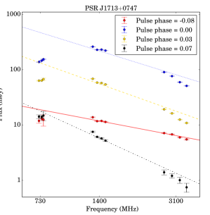
Figure 2: Flux density spectra for PSR J1713$+$0747 at different pulse phases. The best fit power-law spectra are indicated with different types of lines.

Table 6: Flux densities and spectral indices for PPTA MSPs.

PSR	$S_{730}$	$S^{\rm{RMS}}_{730}$	$S_{1400}$	$S^{\rm{RMS}}_{1400}$	$S_{3100}$	$S^{\rm{RMS}}_{3100}$	Spectral index
	(mJy)	(mJy)	(mJy)	(mJy)	(mJy)	(mJy)	$\alpha_{1}$	$\alpha_{2}$
J0437$-$4715	364.3 $\pm$ 19.2	255.2	150.2 $\pm$ 1.6	42.2	35.6 $\pm$ 1.2	20.5	$-$1.69 $\pm$ 0.03	$-$1.65 $\pm$ 0.02
J0613$-$0200	6.7 $\pm$ 0.3	2.3	2.25 $\pm$ 0.03	0.4	0.45 $\pm$ 0.01	0.1	$-$1.90 $\pm$ 0.03	$-$1.83 $\pm$ 0.03
J0711$-$6830	11.4 $\pm$ 1.0	8.5	3.7 $\pm$ 0.4	5.7	0.72 $\pm$ 0.04	0.4	$-$1.94 $\pm$ 0.03	$-$1.83 $\pm$ 0.05
J1017$-$7156	2.5 $\pm$ 0.1	0.8	0.99 $\pm$ 0.04	0.4	0.21 $\pm$ 0.01	0.1	$-$1.67 $\pm$ 0.04	$-$1.64 $\pm$ 0.04
J1022$+$1001	14.2 $\pm$ 2.8	22.9	4.9 $\pm$ 0.4	4.6	1.18 $\pm$ 0.03	0.4	$-$1.66 $\pm$ 0.03	$-$1.91 $\pm$ 0.06
J1024$-$0719	5.6 $\pm$ 0.8	4.9	2.3 $\pm$ 0.2	1.7	0.52 $\pm$ 0.01	0.1	$-$1.80 $\pm$ 0.03	$-$1.62 $\pm$ 0.05
J1045$-$4509	9.2 $\pm$ 0.2	1.8	2.74 $\pm$ 0.04	0.5	0.48 $\pm$ 0.01	0.1	$-$2.06 $\pm$ 0.02	$-$2.04 $\pm$ 0.03
J1446$-$4701	1.8 $\pm$ 0.1	0.5	0.46 $\pm$ 0.02	0.2	0.15 $\pm$ 0.02	0.07	$-$2.05 $\pm$ 0.07	$-$1.93 $\pm$ 0.09
J1545$-$4550			0.87 $\pm$ 0.05	0.2	0.34 $\pm$ 0.04	0.1	$-$1.15 $\pm$ 0.07	$-$1.13 $\pm$ 0.06
J1600$-$3053	2.9 $\pm$ 0.1	0.4	2.44 $\pm$ 0.04	0.4	0.84 $\pm$ 0.02	0.2	$-$0.83 $\pm$ 0.07	$-$1.19 $\pm$ 0.05
J1603$-$7202	10.9 $\pm$ 0.7	4.9	3.5 $\pm$ 0.2	1.7	0.55 $\pm$ 0.06	0.4	$-$2.15 $\pm$ 0.06	$-$2.03 $\pm$ 0.05
J1643$-$1224	12.4 $\pm$ 0.2	1.4	4.68 $\pm$ 0.06	0.7	1.18 $\pm$ 0.02	0.2	$-$1.64 $\pm$ 0.01	$-$1.66 $\pm$ 0.02
J1713$+$0747	10.1 $\pm$ 0.8	6.2	9.1 $\pm$ 0.7	8.4	2.6 $\pm$ 0.2	1.6	$-$1.06 $\pm$ 0.07	$-$1.2 $\pm$ 0.1
J1730$-$2304	11.5 $\pm$ 0.5	3.9	4.0 $\pm$ 0.2	2.0	1.7 $\pm$ 0.2	1.5	$-$1.46 $\pm$ 0.06	$-$1.22 $\pm$ 0.07
J1744$-$1134	8.0 $\pm$ 0.7	5.7	3.2 $\pm$ 0.3	3.2	0.77 $\pm$ 0.05	0.5	$-$1.63 $\pm$ 0.03	$-$1.58 $\pm$ 0.05
J1824$-$2452A	11.4 $\pm$ 0.5	2.9	2.30 $\pm$ 0.05	0.4	0.39 $\pm$ 0.01	0.1	$-$2.28 $\pm$ 0.03	$-$2.35 $\pm$ 0.03
J1832$-$0836			1.18 $\pm$ 0.07	0.3	0.32 $\pm$ 0.03	0.1	$-$1.66 $\pm$ 0.06	$-$1.60 $\pm$ 0.07
J1857$+$0943	10.4 $\pm$ 0.4	3.0	5.1 $\pm$ 0.3	2.9	1.2 $\pm$ 0.1	0.9	$-$1.46 $\pm$ 0.04	$-$1.63 $\pm$ 0.07
J1909$-$3744	4.9 $\pm$ 0.3	3.1	2.5 $\pm$ 0.2	3.2	0.76 $\pm$ 0.04	0.5	$-$1.29 $\pm$ 0.02	$-$1.29 $\pm$ 0.03
J1939$+$2134	67.8 $\pm$ 2.7	20.9	15.2 $\pm$ 0.6	6.2	1.82 $\pm$ 0.09	0.9	$-$2.52 $\pm$ 0.02	$-$2.54 $\pm$ 0.02
J2124$-$3358	19.3 $\pm$ 2.7	17.2	4.5 $\pm$ 0.2	2.2	0.82 $\pm$ 0.01	0.1	$-$2.15 $\pm$ 0.03	$-$2.25 $\pm$ 0.03
J2129$-$5721	5.9 $\pm$ 0.5	3.9	1.28 $\pm$ 0.09	1.0	0.34 $\pm$ 0.05	0.2	$-$2.12 $\pm$ 0.07	$-$2.52 $\pm$ 0.05
J2145$-$0750	27.4 $\pm$ 3.4	28.5	10.3 $\pm$ 1.0	11.2	1.75 $\pm$ 0.07	0.8	$-$1.98 $\pm$ 0.03	$-$1.94 $\pm$ 0.04
J2241$-$5236	11.9 $\pm$ 1.8	16.2	1.95 $\pm$ 0.09	1.2	0.35 $\pm$ 0.01	0.1	$-$2.12 $\pm$ 0.04	$-$2.93 $\pm$ 0.07

4.3 Polarization properties

In Table 7, the fractional linear polarization $\langle L\rangle/S$, the fractional net circular polarization $\langle V\rangle/S$ and the fractional absolute circular polarization $\langle|V|\rangle/S$ at different frequencies are presented. The means are taken across the pulse profile where the total intensity exceeds three times the baseline rms noise. All the polarization parameters are calculated from the average polarization profiles and the uncertainties are estimated using the baseline rms noise (PSRs J1545$-$4550 and J1832$-$0836 have very low S/N profiles in the 50 cm band, therefore we did not present these results in the 50 cm band).

For nine pulsars, we see a clear decrease in the mean fractional linear polarization with increasing frequency. In contrast, for PSRs J1045$-$4509, J1603$-$7202 and J1730$-$2304 and J1824$-$2452A, the mean fractional linear polarization significantly increases with frequency. Different profile components of a pulsar can show different frequency evolution of the fractional linear polarization. For instance, for PSR J1643$-$1224, the fractional linear polarization of the leading edge of the main pulse increases with decreasing frequency while that of the trailing edge decreases with decreasing frequency. There is no evidence that highly polarized sources depolarize rapidly with increasing frequency as reported previously (Kramer et al., 1999a).

Circular polarization also has complicated variations with both frequency and pulse phase, with different components often having different signs of circular polarization and/or opposite frequency dependence in the degree of circular polarization. For example, for PSR J1603$-$7202, the two main components have the same sign of circular polarization, but for the leading component, the circular polarization is much stronger at high frequency, whereas for the trailing component the opposite frequency dependence is seen. For J1017$-$7156, the main peak of the profile has overlapping components, one with negative $V$ and the other with positive $V$. These two components have very different spectral indices, so that at high frequencies the negative $V$ component dominates, whereas at low frequencies, the positive $V$ component, which is slightly narrower, is dominant.

We note that the high fractional linear and circular polarization of pulsars has been suggested as a way to distinguish pulsars from other point radio sources in a continuum survey (e.g., Crawford et al., 2000). However, in continuum surveys the signal is averaged over pulse phases. The Stokes parameters $Q$ and $U$ are initially averaged separately in time and then the average is combined to form the linear polarization. Therefore, the linear polarization of a continuum survey, $L_{\rm{C}}$, is calculated as $\langle L_{\rm{C}}\rangle=\sqrt{\langle Q\rangle^{2}+\langle U\rangle^{2}}$, which is often much less than $\langle L\rangle$ since $Q$ and $U$ can change sign across the profile. In order to aid predictions of the measured linear polarization for MSPs in future continuum surveys we therefore present, in Table 8, the fractional amount of Stokes $Q$ and $U$ and the fractional linear polarization $\langle L_{\rm{C}}\rangle/S$. As expected, these results show that the fractional linear polarization of a pulsar will be reduced in a continuum survey and therefore any predictions for the discovery of pulsars in future continuum surveys should make use of the results in Table 8. We note that the RM and DM for a particular source may not be known at or shortly after the time of a continuum survey, and therefore the fractional linear polarization could be further reduced. However, the circularly polarised flux component should remain unaffected.

The bottom parts of the right-side panels of Fig. 5 to 28 show the phase-resolved fractional linear polarization for each MSP. For most of our MSPs, the phase-resolved fractional linear polarization is remarkably similar at different observing bands (examples include PSR J0437$-$4715 and J1857$+$0943). However, for a few pulsars (such as PSR J1022$+$1001) the fractional linear polarization differs between bands. We find no strong correlation between the phase-resolved spectral index and the fractional linear polarization. In pulsars such as PSRs J1603$-$7202, J1730$-$2304, J1939$+$2134, J2145$-$0750 and J2241$-$5236 we see evidence that the main component has a lower fractional linear polarization than leading or trailing components (e.g., Basu et al., 2015). However, for PSR J1744$-$1134, we do not see high fractional linear polarizations in the precursor pulse.

At phase ranges where a PA transition occurs, the fractional linear polarization is significantly lower than other phase ranges, which can be explained as the overlap of orthogonal modes. However, we do not see significantly lower or higher fractional net circular polarization close to PA transitions. We do not find strong relations between the size of the PA transition and the fractional linear polarization. Orthogonal mode transitions normally correspond to lower fractional linear polarization, but we also see low fractional linear polarizations for non-orthogonal transitions, for instance in PSRs J1045$-$4509 and J1730$-$2304.

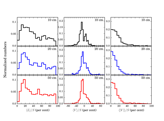
Figure 3: Histograms of the phase-resolved fractional linear, net circular and absolute circular polarization for $24$ MSPs in three bands.

In Fig. 3, the distribution of phase-resolved fractional linear, circular and net circular polarization for 24 MSPs in three bands are shown. To obtain the phase-resolved values, we rebinned the profile in each band into $128$ phase bins and only phase bins whose linear or circular polarization exceeds three times their baseline rms noise were used. While the distributions of the fractional linear polarization are similar across three bands, we see that both the distribution of fractional net circular and absolute circular polarization becomes narrower at lower frequencies. This indicates that the fractional circular and net circular polarization decrease with decreasing frequency.

Table 7: The fractional linear polarization $\langle L\rangle/S$, the fractional net circular polarization $\langle V\rangle/S$ and the fractional absolute circular polarization $\langle|V|\rangle/S$ for 24 PPTA MSPs.

PSR		$\langle L\rangle/S$			$\langle V\rangle/S$			$\langle|V|\rangle/S$
	50 cm	20 cm	10 cm	50 cm	20 cm	10 cm	50 cm	20 cm	10 cm
	(per cent)	(per cent)	(per cent)	(per cent)	(per cent)	(per cent)	(per cent)	(per cent)	(per cent)
J0437$-$4715	26.6 $\pm$ 0.0	25.1 $\pm$ 0.0	20.4 $\pm$ 0.0	$-4.2$ $\pm$ 0.0	$-2.9$ $\pm$ 0.0	$-8.0$ $\pm$ 0.0	15.4 $\pm$ 0.0	11.3 $\pm$ 0.0	12.4 $\pm$ 0.0
J0613$-$0200	28.9 $\pm$ 0.3	21.0 $\pm$ 0.1	14.7 $\pm$ 0.5	$-6.5$ $\pm$ 0.3	$5.2$ $\pm$ 0.1	$10.7$ $\pm$ 0.6	8.9 $\pm$ 0.3	5.6 $\pm$ 0.1	11.2 $\pm$ 0.6
J0711$-$6830	24.6 $\pm$ 0.2	14.1 $\pm$ 0.1	17 $\pm$ 2	$-12.7$ $\pm$ 0.2	$-12.9$ $\pm$ 0.1	$-24$ $\pm$ 2	12.7 $\pm$ 0.2	13.1 $\pm$ 0.1	24 $\pm$ 2
J1017$-$7156	44.5 $\pm$ 0.7	35.4 $\pm$ 0.3	42 $\pm$ 1	$6.9$ $\pm$ 0.8	$-28.9$ $\pm$ 0.2	$-38$ $\pm$ 2	18.5 $\pm$ 0.8	29.5 $\pm$ 0.2	42 $\pm$ 2
J1022$+$1001	67.9 $\pm$ 0.1	56.3 $\pm$ 0.0	23.5 $\pm$ 0.2	$-13.4$ $\pm$ 0.1	$-11.6$ $\pm$ 0.0	$-2.7$ $\pm$ 0.2	13.4 $\pm$ 0.1	12.6 $\pm$ 0.0	5.6 $\pm$ 0.2
J1024$-$0719	69.0 $\pm$ 0.6	67.9 $\pm$ 0.1	61.7 $\pm$ 0.8	$1.1$ $\pm$ 0.6	$5.5$ $\pm$ 0.2	$6.1$ $\pm$ 0.7	3.7 $\pm$ 0.6	6.3 $\pm$ 0.2	6.7 $\pm$ 0.7
J1045$-$4509	18.7 $\pm$ 0.3	22.5 $\pm$ 0.1	30.2 $\pm$ 0.5	$8.2$ $\pm$ 0.3	$14.7$ $\pm$ 0.1	$16.4$ $\pm$ 0.6	10.6 $\pm$ 0.3	16.6 $\pm$ 0.1	16.5 $\pm$ 0.6
J1446$-$4701	60.4 $\pm$ 2.8	38 $\pm$ 1	0.0 $\pm$ 3.5	$-13$ $\pm$ 2	$-9$ $\pm$ 1	$0.0$ $\pm$ 3.1	15 $\pm$ 3	11 $\pm$ 1	0.0 $\pm$ 3.1
J1545$-$4550		58 $\pm$ 1	59 $\pm$ 2		$-13.2$ $\pm$ 0.9	$-10$ $\pm$ 2		17.1 $\pm$ 0.9	11 $\pm$ 2
J1600$-$3053	33 $\pm$ 2	31.3 $\pm$ 0.1	36.8 $\pm$ 0.3	$0.4$ $\pm$ 2	$3.8$ $\pm$ 0.1	$-2.3$ $\pm$ 0.3	3 $\pm$ 2	4.0 $\pm$ 0.1	4.7 $\pm$ 0.3
J1603$-$7202	16.6 $\pm$ 0.2	18.6 $\pm$ 0.1	31.6 $\pm$ 0.7	$33.6$ $\pm$ 0.3	$29.0$ $\pm$ 0.1	$15.3$ $\pm$ 0.8	34.2 $\pm$ 0.3	32.4 $\pm$ 0.1	22.3 $\pm$ 0.8
J1643$-$1224	20.0 $\pm$ 0.3	17.4 $\pm$ 0.1	19.9 $\pm$ 0.2	$6.8$ $\pm$ 0.2	$0.4$ $\pm$ 0.1	$-6.6$ $\pm$ 0.2	13.9 $\pm$ 0.2	13.8 $\pm$ 0.1	10.4 $\pm$ 0.2
J1713$+$0747	33.3 $\pm$ 0.3	31.5 $\pm$ 0.0	27.0 $\pm$ 0.1	$-2.8$ $\pm$ 0.2	$1.1$ $\pm$ 0.0	$-1.1$ $\pm$ 0.1	3.9 $\pm$ 0.2	3.8 $\pm$ 0.0	3.8 $\pm$ 0.1
J1730$-$2304	26.2 $\pm$ 0.3	29.2 $\pm$ 0.1	44.9 $\pm$ 0.2	$-19.1$ $\pm$ 0.3	$-19.4$ $\pm$ 0.1	$-11.9$ $\pm$ 0.2	19.2 $\pm$ 0.3	20.6 $\pm$ 0.1	15.9 $\pm$ 0.2
J1744$-$1134	88.9 $\pm$ 0.4	91.8 $\pm$ 0.1	88.0 $\pm$ 0.4	$0.2$ $\pm$ 0.4	$2.9$ $\pm$ 0.1	$1.5$ $\pm$ 0.3	0.7 $\pm$ 0.4	2.9 $\pm$ 0.1	1.6 $\pm$ 0.3
J1824$-$2452A	70.9 $\pm$ 0.5	77.8 $\pm$ 0.2	84.2 $\pm$ 1.0	$0.1$ $\pm$ 0.3	$3.5$ $\pm$ 0.2	$-0.8$ $\pm$ 0.8	3.8 $\pm$ 0.3	4.4 $\pm$ 0.2	5.5 $\pm$ 0.8
J1832$-$0836		36 $\pm$ 2	43 $\pm$ 11		$3$ $\pm$ 1	$-4$ $\pm$ 10		10 $\pm$ 1	11 $\pm$ 10
J1857$+$0943	20.9 $\pm$ 0.9	14.5 $\pm$ 0.1	14.1 $\pm$ 0.4	$-1.2$ $\pm$ 0.7	$2.5$ $\pm$ 0.1	$0.3$ $\pm$ 0.4	4.7 $\pm$ 0.7	5.8 $\pm$ 0.1	7.3 $\pm$ 0.4
J1909$-$3744	61.2 $\pm$ 0.4	48.7 $\pm$ 0.1	26.3 $\pm$ 0.2	$13.1$ $\pm$ 0.4	$14.9$ $\pm$ 0.1	$5.0$ $\pm$ 0.2	15.4 $\pm$ 0.4	16.1 $\pm$ 0.1	6.6 $\pm$ 0.2
J1939$+$2134	38.1 $\pm$ 0.1	30.0 $\pm$ 0.0	24.3 $\pm$ 0.2	$0.9$ $\pm$ 0.1	$3.3$ $\pm$ 0.0	$-0.2$ $\pm$ 0.2	1.1 $\pm$ 0.1	3.3 $\pm$ 0.0	1.2 $\pm$ 0.2
J2124$-$3358	46.2 $\pm$ 0.2	33.1 $\pm$ 0.1	49 $\pm$ 1	$-2.5$ $\pm$ 0.2	$0.4$ $\pm$ 0.1	$-3.9$ $\pm$ 1.0	3.8 $\pm$ 0.2	5.5 $\pm$ 0.1	7 $\pm$ 1
J2129$-$5721	66.8 $\pm$ 0.6	47.3 $\pm$ 0.2	39 $\pm$ 8	$-27.0$ $\pm$ 0.6	$-24.8$ $\pm$ 0.2	$-16$ $\pm$ 8	35.5 $\pm$ 0.6	26.6 $\pm$ 0.2	17 $\pm$ 8
J2145$-$0750	19.2 $\pm$ 0.1	15.9 $\pm$ 0.0	10.9 $\pm$ 0.1	$5.9$ $\pm$ 0.1	$9.2$ $\pm$ 0.0	$0.9$ $\pm$ 0.1	9.5 $\pm$ 0.1	10.0 $\pm$ 0.0	8.1 $\pm$ 0.1
J2241$-$5236	20.0 $\pm$ 0.2	12.6 $\pm$ 0.1	12.5 $\pm$ 0.7	$-2.9$ $\pm$ 0.2	$-0.7$ $\pm$ 0.1	$-4.2$ $\pm$ 0.7	4.7 $\pm$ 0.2	6.2 $\pm$ 0.1	8.9 $\pm$ 0.7

Table 8: The fractional amount of Stokes $Q$ and $U$ and the fractional linear polarization $\langle L_{\rm{C}}\rangle/S$ for 24 PPTA MSPs.

PSR		$\langle Q\rangle/S$			$\langle U\rangle/S$			$\langle L_{\rm{C}}\rangle/S$
	50 cm	20 cm	10 cm	50 cm	20 cm	10 cm	50 cm	20 cm	10 cm
	(per cent)	(per cent)	(per cent)	(per cent)	(per cent)	(per cent)	(per cent)	(per cent)	(per cent)
J0437$-$4715	$-3.0$ $\pm$ 0.0	$-1.8$ $\pm$ 0.0	$0.2$ $\pm$ 0.0	$0.7$ $\pm$ 0.0	$-4.3$ $\pm$ 0.0	$0.9$ $\pm$ 0.0	3.0 $\pm$ 0.0	4.7 $\pm$ 0.0	0.9 $\pm$ 0.0
J0613$-$0200	$9.9$ $\pm$ 0.3	$8.9$ $\pm$ 0.1	$6.1$ $\pm$ 0.4	$-6.9$ $\pm$ 0.3	$8.3$ $\pm$ 0.1	$-3.1$ $\pm$ 0.4	12.1 $\pm$ 0.3	12.1 $\pm$ 0.1	6.8 $\pm$ 0.4
J0711$-$6830	$-14.1$ $\pm$ 0.2	$-6.2$ $\pm$ 0.1	$-1.0$ $\pm$ 0.3	$7.0$ $\pm$ 0.1	$-1.0$ $\pm$ 0.1	$0.6$ $\pm$ 0.3	15.7 $\pm$ 0.2	6.3 $\pm$ 0.1	1.2 $\pm$ 0.3
J1017$-$7156	$23.6$ $\pm$ 0.7	$-17.9$ $\pm$ 0.2	$-22.2$ $\pm$ 1.2	$-22.2$ $\pm$ 0.7	$22.3$ $\pm$ 0.3	$31.2$ $\pm$ 1.3	32.4 $\pm$ 0.7	28.6 $\pm$ 0.3	38.4 $\pm$ 1.3
J1022$+$1001	$14.6$ $\pm$ 0.1	$28.5$ $\pm$ 0.0	$18.1$ $\pm$ 0.2	$22.7$ $\pm$ 0.1	$8.4$ $\pm$ 0.1	$-0.5$ $\pm$ 0.2	27.0 $\pm$ 0.1	29.7 $\pm$ 0.1	18.1 $\pm$ 0.2
J1024$-$0719	$-20.8$ $\pm$ 0.5	$-49.3$ $\pm$ 0.1	$-30.6$ $\pm$ 0.4	$42.1$ $\pm$ 0.5	$27.4$ $\pm$ 0.1	$14.9$ $\pm$ 0.5	47.0 $\pm$ 0.5	56.4 $\pm$ 0.1	34.1 $\pm$ 0.5
J1045$-$4509	$-6.9$ $\pm$ 0.2	$8.6$ $\pm$ 0.1	$0.2$ $\pm$ 0.4	$-9.6$ $\pm$ 0.3	$-8.7$ $\pm$ 0.1	$-14.6$ $\pm$ 0.4	11.8 $\pm$ 0.3	12.2 $\pm$ 0.1	14.6 $\pm$ 0.4
J1446$-$4701	$34.6$ $\pm$ 2.1	$1.7$ $\pm$ 1.0	$6.6$ $\pm$ 4.2	$-36.2$ $\pm$ 2.2	$28.8$ $\pm$ 0.9	$12.3$ $\pm$ 4.1	50.1 $\pm$ 2.2	28.8 $\pm$ 0.9	14.0 $\pm$ 4.1
J1545$-$4550		$-14.9$ $\pm$ 0.8	$-40.3$ $\pm$ 1.7		$-32.5$ $\pm$ 0.6	$-12.4$ $\pm$ 1.5		35.7 $\pm$ 0.7	42.2 $\pm$ 1.7
J1600$-$3053	$-4.4$ $\pm$ 0.9	$-5.7$ $\pm$ 0.1	$2.1$ $\pm$ 0.3	$-18.0$ $\pm$ 1.0	$-5.3$ $\pm$ 0.1	$-16.0$ $\pm$ 0.3	18.5 $\pm$ 1.0	7.8 $\pm$ 0.1	16.1 $\pm$ 0.3
J1603$-$7202	$-3.5$ $\pm$ 0.2	$-2.5$ $\pm$ 0.1	$-10.0$ $\pm$ 0.5	$-3.1$ $\pm$ 0.3	$0.4$ $\pm$ 0.1	$0.5$ $\pm$ 0.5	4.7 $\pm$ 0.2	2.5 $\pm$ 0.1	10.0 $\pm$ 0.5
J1643$-$1224	$12.9$ $\pm$ 0.2	$2.3$ $\pm$ 0.1	$4.5$ $\pm$ 0.2	$-5.3$ $\pm$ 0.2	$-2.7$ $\pm$ 0.1	$0.6$ $\pm$ 0.2	14.0 $\pm$ 0.2	3.5 $\pm$ 0.1	4.5 $\pm$ 0.2
J1713$+$0747	$-9.4$ $\pm$ 0.3	$-2.9$ $\pm$ 0.0	$-2.0$ $\pm$ 0.1	$11.9$ $\pm$ 0.3	$4.2$ $\pm$ 0.0	$6.0$ $\pm$ 0.1	15.2 $\pm$ 0.3	5.1 $\pm$ 0.0	6.4 $\pm$ 0.1
J1730$-$2304	$9.4$ $\pm$ 0.2	$-11.6$ $\pm$ 0.1	$-19.0$ $\pm$ 0.2	$13.3$ $\pm$ 0.3	$19.3$ $\pm$ 0.1	$18.2$ $\pm$ 0.2	16.3 $\pm$ 0.3	22.5 $\pm$ 0.1	26.3 $\pm$ 0.2
J1744$-$1134	$-70.5$ $\pm$ 0.4	$-48.7$ $\pm$ 0.1	$-28.7$ $\pm$ 0.3	$34.8$ $\pm$ 0.4	$67.7$ $\pm$ 0.1	$69.3$ $\pm$ 0.4	78.6 $\pm$ 0.4	83.4 $\pm$ 0.1	75.0 $\pm$ 0.4
J1824$-$2452A	$-34.7$ $\pm$ 0.5	$-19.0$ $\pm$ 0.2	$-33.9$ $\pm$ 0.9	$26.8$ $\pm$ 0.4	$43.2$ $\pm$ 0.1	$35.3$ $\pm$ 0.6	43.8 $\pm$ 0.5	47.2 $\pm$ 0.1	48.9 $\pm$ 0.8
J1832$-$0836		$-1.2$ $\pm$ 0.9	$-15.4$ $\pm$ 2.1		$2.8$ $\pm$ 0.8	$-8.8$ $\pm$ 2.2		3.1 $\pm$ 0.8	17.7 $\pm$ 2.1
J1857$+$0943	$2.0$ $\pm$ 0.5	$0.3$ $\pm$ 0.1	$0.3$ $\pm$ 0.3	$0.9$ $\pm$ 0.4	$-0.6$ $\pm$ 0.1	$4.8$ $\pm$ 0.3	2.2 $\pm$ 0.5	0.6 $\pm$ 0.1	4.8 $\pm$ 0.3
J1909$-$3744	$-54.0$ $\pm$ 0.4	$-42.9$ $\pm$ 0.1	$-23.5$ $\pm$ 0.3	$-12.9$ $\pm$ 0.4	$-15.1$ $\pm$ 0.1	$-9.9$ $\pm$ 0.2	55.5 $\pm$ 0.4	45.4 $\pm$ 0.1	25.5 $\pm$ 0.3
J1939$+$2134	$-30.5$ $\pm$ 0.1	$2.0$ $\pm$ 0.0	$0.1$ $\pm$ 0.2	$-11.8$ $\pm$ 0.1	$16.2$ $\pm$ 0.0	$-6.9$ $\pm$ 0.2	32.7 $\pm$ 0.1	16.3 $\pm$ 0.0	6.9 $\pm$ 0.2
J2124$-$3358	$19.4$ $\pm$ 0.1	$9.0$ $\pm$ 0.1	$-2.0$ $\pm$ 0.4	$8.2$ $\pm$ 0.2	$10.6$ $\pm$ 0.1	$5.4$ $\pm$ 0.5	21.1 $\pm$ 0.2	13.9 $\pm$ 0.1	5.8 $\pm$ 0.5
J2129$-$5721	$22.2$ $\pm$ 0.5	$-24.4$ $\pm$ 0.2	$-3.1$ $\pm$ 2.1	$45.1$ $\pm$ 0.5	$29.6$ $\pm$ 0.2	$16.4$ $\pm$ 2.2	50.2 $\pm$ 0.5	38.3 $\pm$ 0.2	16.7 $\pm$ 2.2
J2145$-$0750	$-5.9$ $\pm$ 0.1	$-2.0$ $\pm$ 0.0	$2.5$ $\pm$ 0.1	$6.2$ $\pm$ 0.1	$3.2$ $\pm$ 0.0	$2.3$ $\pm$ 0.1	8.6 $\pm$ 0.1	3.8 $\pm$ 0.0	3.3 $\pm$ 0.1
J2241$-$5236	$7.8$ $\pm$ 0.2	$0.4$ $\pm$ 0.1	$8.5$ $\pm$ 0.7	$-14.2$ $\pm$ 0.2	$5.0$ $\pm$ 0.1	$-3.8$ $\pm$ 0.7	16.2 $\pm$ 0.2	5.0 $\pm$ 0.1	9.3 $\pm$ 0.7

4.4 Rotation measures

With the aligned, three-band profiles, we can not only determine new RM values, but also investigate whether the polarization PAs obey the expected $\lambda^{2}$ law. To gain enough S/N, we typically split the 10 cm and 20 cm bands into four subbands and the 50 cm band into three subbands. For pulsars whose linear polarization is weak and has low S/N, we split the bands into fewer subbands or fully average them in frequency (specific comments are given in the footnotes of Table 9). For PSR J1832$-$0836, the S/N of profile is low and the linear polarization is weak in both 10 cm and 50 cm bands, therefore we excluded it from our RM measurements.

As the PAs vary significantly with pulse phase and also with observing frequency, we have selected small regions in pulse phase in which the PAs are generally stable across the three bands. Phase ranges we used for each pulsar are listed in the third column of Table 9. In order to avoid low S/N regions and obtain smaller uncertainties of the PA, only phase bins whose linear polarization exceeds five times the baseline rms noise were used.

Our results are summarised in Table 9. Previously published results, obtained from the 20 cm band alone, are shown in the second column. In columns 3, 4 and 5 we present our results determined across two bands (10-20, 10-50 and 20-50 respectively). In column 6 we present the RM value obtained by fitting across all three bands. In Fig. 4, the mean PAs in the stable regions for each pulsar are plotted a function of $\lambda^{2}$. The best fitted RMs are indicated with red dashed lines.

For some pulsars, our RMs are significantly different from previously published results. These are explained as follows. First, previous measurements were obtained using only the 20 cm band. In Fig. 4 it is clear that for pulsars such as J0437$-$4715, J1022$+$1001 and J1744$-$1134, the PAs in the 20 cm band deviate from the best fitted lines obtained using the wider band. Second, previous measurements used PAs averaged over the pulse longitude while we only averaged PAs within phase ranges that PAs are stable. Therefore, the variation of RM across the pulse longitude would introduce deviations.

Fig. 4 shows that, for some pulsars, the PAs generally obey the $\lambda^{2}$ fit across a wide range of frequency (e.g., PSRs J0613$-$0200, J0711$-$6830, J1045$-$4509, J1643$-$1224, J1824$-$2452A). However, for other pulsars, the PAs can significantly deviate from the $\lambda^{2}$ fit across bands (e.g., PSRs J1017$-$7156, J1713$+$0747) and show different trends within bands (e.g., PSRs J0437$-$4715, J1022$+$1001, J1730$-$2304, J1744$-$1134, J1909$-$3744, J2124$-$3358, J2145$-$0750). For PSRs J2124$-$3358 and J2129$-$5721, the deviation of PA in the 10 cm band from the best fitted result is likely caused by the low S/N of the profile. For PSRs J1603$-$7202 and J2145$-$0750, the PA curves vary dramatically within bands and cause the deviation of PAs from the $\lambda^{2}$ fit.

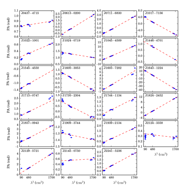
Figure 4: Position angles as a function of $\lambda^{2}$ for $23$ MSPs. The fitted RMs are indicated with red dashed lines. PSR J1832$-$0836 is not included here because of the low S/N in the 10 cm and 50 cm bands for this pulsar.

Table 9: Interstellar RMs for $23$ MSPs in units of $\rm{rad\ m^{-2}}$. Previoulsy published results without footnotes are from Yan et al. (2011a).

PSR	Previously published	Phase ranges	Measured from mean profile
	20 cm		10 cm - 20 cm	10 cm - 50 cm	20 cm - 50 cm	fitting
J0437$-$4715	$0.0$ $\pm$ 0.4	$(0.01,0.03)$	$0.60$$\pm$ 0.01	$0.618$$\pm$ 0.004	$0.624$$\pm$ 0.001	$0.58$$\pm$ 0.09
J0613$-$0200⋆	$9.7$ $\pm$ 1.1	$(0.01,0.03)$	$19.8$$\pm$ 0.7	$17.8$$\pm$ 0.2	$17.20$$\pm$ 0.08	$17.5$$\pm$ 0.3
J0711$-$6830	$21.6$ $\pm$ 3.1	$(-0.28,-0.26)$	$22.1$$\pm$ 0.4	$23.5$$\pm$ 0.1	$23.89$$\pm$ 0.05	$23.9$$\pm$ 0.4
J1017$-$7156	$-78$ $\pm$ $3^{a}$	$(-0.025,0.005)$	$-82.1$$\pm$ 0.2	$-66.59$$\pm$ 0.04	$-61.66$$\pm$ 0.03	$-63$$\pm$ 1
J1022$+$1001	$-0.6$ $\pm$ 0.5	$(-0.01,0.01)$	$4.68$$\pm$ 0.06	$2.95$$\pm$ 0.01	$2.405$$\pm$ 0.004	$2.4$$\pm$ 0.1
J1024$-$0719	$-8.2$ $\pm$ 0.8	$(-0.04,0.03)$	$-1.88$$\pm$ 0.09	$-2.26$$\pm$ 0.03	$-2.38$$\pm$ 0.02	$-2.4$$\pm$ 0.2
J1045$-$4509	$92.0$ $\pm$ 1.0	$(0.05,0.07)$	$91.5$$\pm$ 0.1	$93.34$$\pm$ 0.06	$93.91$$\pm$ 0.07	$94.7$$\pm$ 0.7
J1446$-$4701∗	$-14$ $\pm$ $3^{a}$	$(-0.05,0.0)$			$-8.98$$\pm$ 0.11	$-9.1$$\pm$ 0.2
J1545$-$4550†	$-0.6$ $\pm$ $1.3^{b}$	$(-0.05,0.0)$	$6.3$$\pm$ 0.2			$6.1$$\pm$ 0.5
J1600$-$3053	$-15.5$ $\pm$ 1.0	$(0.01,0.04)$	$-11.6$$\pm$ 0.1	$-11.77$$\pm$ 0.09	$-11.8$$\pm$ 0.1	$-11.8$$\pm$ 0.3
J1603$-$7202	$27.7$ $\pm$ 0.8	$(-0.01,0.0)$	$31.2$$\pm$ 0.4	$28.91$$\pm$ 0.09	$28.20$$\pm$ 0.05	$35$$\pm$ 2
J1643$-$1224	$-308.1$ $\pm$ 1.0	$(-0.1,-0.05)$	$-306.8$$\pm$ 0.2	$-301.70$$\pm$ 0.06	$-300.09$$\pm$ 0.05	$-305.7$$\pm$ 0.2
J1713$+$0747	$8.4$ $\pm$ 0.6	$(0.0,0.01)$	$8.19$$\pm$ 0.02	$10.67$$\pm$ 0.02	$11.45$$\pm$ 0.03	$8.7$$\pm$ 0.5
J1730$-$2304	$-7.2$ $\pm$ 2.2	$(-0.02,0.0)$	$-13.4$$\pm$ 0.2	$-9.22$$\pm$ 0.08	$-7.88$$\pm$ 0.1	$-8.8$$\pm$ 0.6
J1744$-$1134	$-1.6$ $\pm$ 0.7	$(0.0,0.02)$	$3.24$$\pm$ 0.02	$2.34$$\pm$ 0.01	$2.05$$\pm$ 0.01	$2.2$$\pm$ 0.2
J1824$-$2452A	$77.8$ $\pm$ 0.6	$(-0.02,0.04)$	$82.6$$\pm$ 0.3	$82.06$$\pm$ 0.07	$81.91$$\pm$ 0.04	$82.2$$\pm$ 0.2
J1857$+$0943‡	$16.4$ $\pm$ 3.5	$(0.06,0.062)$	$18.4$$\pm$ 0.8	$21.4$$\pm$ 0.3	$22.4$$\pm$ 0.3	$22.2$$\pm$ 0.9
J1909$-$3744	$-6.6$ $\pm$ 0.8	$(-0.01,0.01)$	$-0.38$$\pm$ 0.02	$-0.30$$\pm$ 0.01	$-0.27$$\pm$ 0.01	$-0.6$$\pm$ 0.2
J1939$+$2134	$6.7$ $\pm$ 0.6	$(0.0,0.04)$	$12.3$$\pm$ 0.2	$9.13$$\pm$ 0.05	$8.11$$\pm$ 0.01	$8.3$$\pm$ 0.1
J2124$-$3358	$-5.0$ $\pm$ 0.9	$(-0.4,-0.38)$	$1.6$$\pm$ 0.3	$0.07$$\pm$ 0.08	$-0.41$$\pm$ 0.03	$-0.4$$\pm$ 0.1
J2129$-$5721∐	$23.5$ $\pm$ 0.8	$(-0.02,0.0)$	$0.00$$\pm$ 0.06	$16.61$$\pm$ 0.02	$21.88$$\pm$ 0.03	$22.3$$\pm$ 0.3
J2145$-$0750	$-1.3$ $\pm$ 0.7	$(-0.03,-0.01)$	$1.4$$\pm$ 0.3	$-0.31$$\pm$ 0.09	$-0.85$$\pm$ 0.04	$-0.8$$\pm$ 0.1
J2241$-$5236	$14$ $\pm$ $6^{c}$	$(0.02,0.04)$	$16.1$$\pm$ 0.3	$13.84$$\pm$ 0.08	$13.14$$\pm$ 0.04	$13.3$$\pm$ 0.1

^a Keith et al. (2012); ^b Burgay et al. (2013); ^c Keith et al. (2011).  
^⋆ J0613$-$0200: 50 cm, two subbands; 10 cm, one subband.  
^∗ J1446$-$4701: 50 cm, one subband; 10 cm, not used.  
^† J1545$-$4550: 50 cm, not used.  
^‡ J1857$+$0943: 50 cm, two subband.  
^∐ J2129$-$5721: 10 cm, one subband..

The bottom parts of the right-side panels of Fig. 5 to 28 show measurements of apparent RM measured at specific phases for each MSP. Since only phase bins whose linear polarization exceeds five times the baseline rms noise were used, and we only plot RMs whose uncertainty is smaller than $3\ \rm{rad\ m^{-2}}$, the phase-resolved RMs only cover pulse phases where the linear polarization is strong and PAs generally obey the $\lambda^{2}$ fit. For most pulsars, we can see systematic RM variations across the pulse longitude following the structure of the mean profile. For instance, in PSR J0437$-$4715 the RM shows complex variations from approximately $-8\ \rm{rad\ m^{-2}}$ to $8\ \rm{rad\ m^{-2}}$. For PSR J1643$-$1224, one linear polarization component has a RM of approximately $-306\ \rm{rad\ m^{-2}}$ and the other $-300\ \rm{rad\ m^{-2}}$. We find that in some cases significant RM variations are associated with orthogonal or non-orthogonal mode transitions in PA (e.g., PSRs J1022$+$1001, J1600$-$3053, J1643$-$1224, J1713$+$0747). For PSR J1744$-$1134, whose PA curve is smooth across the main pulse, the RMs show minor variations. This is consistent with previous phase-resolved RM study of normal pulsars, which also shows that the greatest RM fluctuations seem coincident with the steepest gradients of the PA curve, whereas pulsars with flat PA curve show little RM variation (Noutsos et al., 2009).

5 Summary of results and conclusions

Our results indicate that:

• Most MSPs in our sample have very wide profiles with multiple components. This is not a surprise and has been presented in numerous earlier publications. We have shown that 18 of the 24 MSPs exhibit emission over more than half of the pulse period and the overall pulse width is relatively constant for pulsars that have high S/N profiles in all three bands. The MSPs in our sample do not show the frequency evolution of the component separations (Kramer et al., 1999a) that has been observed in normal pulsars (e.g., Cordes, 1978; Thorsett, 1991; Mitra & Rankin, 2002; Mitra & Li, 2004; Chen & Wang, 2014).

• The spectra for some of the pulsars in our sample significantly deviate from a single power-law across the different observing bands. We have observed the spectral steepening at high frequencies and, for some pulsars, we have shown positive spectral indices in the 50 cm band. We have also observed the spectral flattening within bands at high frequencies for PSRs J1022$+$1001 and J2241$-$5236. The spectral steepening and turnover have been identified in normal pulsars (e.g., Maron et al., 2000; Kijak et al., 2011). The flattening or turn-up of the spectrum has been previously observed at extremely high frequencies ($\sim 30$ GHz) (Kramer et al., 1996), and has been explained by refraction effects (Petrova, 2002). However, such spectral features have not been observed in MSPs before, and previous measurements of MSP flux densities over a wide frequency range did not show spectral turnovers or breaks (Kramer et al., 1999a; Kuzmin & Losovsky, 2001).

• For almost all of the MSPs in our sample, the observed three-band PA variations across the profile are extremely complicated and cannot be fitted using the RVM. We show complex details of the PA variation for several MSPs, which were previously thought to have relatively flat or smooth PA profiles (e.g., PSRs J1024$-$0719, J1600$-$3053, J1744$-$1134, J2124$-$3358). Across bands, the PA profiles can evolve significantly (e.g., PSRs J0437$-$4715, J0711$-$6830, J1603$-$7202, J1730$-$2304).

  One exception is PSR J1022$+$1001, whose PA profile is relatively smooth in all three bands except for a discontinuity close to phase zero. At 10 cm, the PA variation fits the RVM very well. The PA variation departs from the RVM progressively with decreasing frequency. One model to explain this would be that at higher frequencies and lower emission heights, the magnetic field is closer to a simple dipolar field. As the frequency decreases, the magnetic field departs from this simple dipolar form. It is worth noting that PSR J1022$+$1001 has the longest pulse period of the pulsars in our sample.

• We have observed systematic variations of apparent RM across the pulse longitude following the structure of the mean profile, indicating that such variations are likely to arise from the pulsar magnetosphere. We have also shown that the PA of some pulsars does not follow the $\lambda^{2}$ relation. As discussed in Noutsos et al. (2009), possible explanations of these phenomena includes Faraday rotation in the pulsar magnetosphere (Kennett & Melrose, 1998; Wang et al., 2011), the superposition and frequency dependence of quasi-orthogonal polarization modes (Ramachandran et al., 2004) and interstellar scattering (Karastergiou, 2009).

• Different pulse components usually have differing spectral indices, apparent RMs and fractional polarizations. Measurements of flux density as a function of frequency for individual components can significantly differ from that obtained by averaging over the entire profile. The spectral shape also often deviates from a single power-law. In some cases, the peaks of pulse components coincide with the local maximum or minimum of the phase-resolved spectral index. The fractional polarization increases with increasing frequency for some components, but decreases for other components. These results suggest that there are multiple emission regions or structures within the pulsar magnetosphere and that pulse components originate in different locations within the magnetosphere (e.g., Dyks et al., 2010).

The main goal of this paper has been to inspire and promote our studies and understanding of the MSP emission mechanism by publishing high quality, multi-frequency polarization profiles. All the raw data and resulting averaged profiles are available for public access online.

Producing a model to describe all these observations will be extremely challenging and made more-so by the gaps in the frequency coverage that we currently have available at the Parkes telescope. In order to mitigate this problem, we are developing a new ultra-wideband receiver system that will provide simultaneous observations from approximately $0.7$ to $4$ GHz. As our telescope sensitivity continues to improve, millisecond pulsar profiles seem to become more and more complicated. However, it is still likely that even more low-level components exist in these pulsars. A full understanding of the pulse profiles will only be possible with the sensitivity provided by future telescopes such as the five-hundred-metre-spherical telescope (FAST) and the Square Kilometre Array (SKA).

Appendix A Multi-frequency Polarization Profiles

Table 10: References, duty cycles and S/N for MSPs in our sample.

PSR	References	Duty cycle	S/N
			50 cm	20 cm	10 cm
J0437$-$4715	Johnston et al. (1993); Manchester & Johnston (1995)	0.05	14285.8	33512.4	5445.6
	Navarro et al. (1997); Yan et al. (2011a)
J0613$-$0200	Xilouris et al. (1998); Stairs et al. (1999)	0.2	812.3	1490.1	396.5
	Ord et al. (2004); Yan et al. (2011a)
J0711$-$6830	Manchester & Han (2004); Ord et al. (2004); Yan et al. (2011a)	0.05	1194.0	3368.4	488.8
J1017$-$7156	Keith et al. (2012)	0.2	634.4	1057.0	233.6
J1022$+$1001	Xilouris et al. (1998); Kramer et al. (1999b)	0.2	4827.2	6979.8	1577.0
	Stairs et al. (1999); Ord et al. (2004); Yan et al. (2011a)
J1024$-$0719	Xilouris et al. (1998); Ord et al. (2004); Yan et al. (2011a)	0.05	613.0	1459.8	273.6
J1045$-$4509	Manchester & Han (2004); Ord et al. (2004); Yan et al. (2011a)	0.2	1097.4	2155.7	456.8
J1446$-$4701	Keith et al. (2012)	0.2	62.2	215.2	31.6
J1545$-$4550	Burgay et al. (2013)	0.2		203.5	157.8
J1600$-$3053	Ord et al. (2004); Yan et al. (2011a)	0.2	213.6	2158.3	1045.2
J1603$-$7202	Manchester & Han (2004); Ord et al. (2004); Yan et al. (2011a)	0.2	1603.6	3215.6	446.8
J1643$-$1224	Xilouris et al. (1998); Stairs et al. (1999)	0.2	1505.3	3097.7	1073.4
	Ord et al. (2004); Yan et al. (2011a)
J1713$+$0747	Xilouris et al. (1998); Stairs et al. (1999)	0.2	1751.4	10294.1	3894.0
	Ord et al. (2004); Yan et al. (2011a)
J1730$-$2304	Xilouris et al. (1998); Kramer et al. (1998)	0.2	1138.4	2645.2	1665.1
	Stairs et al. (1999); Ord et al. (2004); Yan et al. (2011a)
J1744$-$1134	Xilouris et al. (1998); Kramer et al. (1998)	0.2	1808.5	4516.1	1025.0
	Stairs et al. (1999); Ord et al. (2004); Yan et al. (2011a)
J1824$-$2452A	Ord et al. (2004); Yan et al. (2011a); Stairs et al. (1999)	0.05	432.2	620.0	136.3
J1832$-$0836	Burgay et al. (2013)	0.2		100.8	24.2
J1857$+$0943	Thorsett & Stinebring (1990); Xilouris et al. (1998)	0.2	376.7	1563.0	498.9
	Ord et al. (2004); Yan et al. (2011a)
J1909$-$3744	Ord et al. (2004); Yan et al. (2011a)	0.2	1702.4	9413.7	1971.3
J1939$+$2134	Thorsett & Stinebring (1990); Xilouris et al. (1998)	0.2	2066.5	1562.6	565.0
	Stairs et al. (1999); Ord et al. (2004); Yan et al. (2011a)
J2124$-$3358	Manchester & Han (2004); Ord et al. (2004); Yan et al. (2011a)	0.05	332.2	411.0	135.4
J2129$-$5721	Manchester & Han (2004); Ord et al. (2004); Yan et al. (2011a)	0.2	750.6	1829.3	59.5
J2145$-$0750	Xilouris et al. (1998); Stairs et al. (1999)	0.2	4051.6	8680.7	1483.6
	Manchester & Han (2004); Ord et al. (2004); Yan et al. (2011a)
J2241$-$5236	Keith et al. (2011)	0.2	4270.2	3549.0	311.0

In this section, we present the multi-frequency polarization pulse profiles and phase-resolved results for each MSP in Figures 5 to 28. The left-hand panels show the pulse profile in the 10 cm (top), 20 cm (second panel) and 50 cm (third panel) observing bands. The black, blue and red lines in these panels respectively indicate the total intensity, Stokes I, profile in the three bands. The yellow line indicates linear polarization and the grey line shows circular polarization. The bottom panel on the left-hand side presents the phase-resolved spectral index. The red dashed line and yellow highlighted region represent the measured spectral index and its uncertainty as presented in Table 6. In the right-hand panels we have two panels for each of the 10 cm, 20 cm and 50 cm bands. The upper panel shows the position angle of the linear polarization at the band central frequency (in degrees). The lower panels shows a zoom-in around the profile baseline to show weak profile features. The colour scheme is the same as in the left-hand panels. The bottom two panels on the right-hand side show the phase-resolved fractional linear polarization for the three observing bands using the same colour scheme as above, and the phase-resolved RM. The red dashed line and yellow highlighted region represent the measured RM value and its uncertainty. In all panels, vertical dashed lines show the positions of peaks in the 20 cm total intensity profile.

In Table 10, we give the references, baseline duty cycle and S/N for the pulse profile in each band for each pulsar. Specific comments for each individual pulsar and on the comparison with previous work are given in the caption of each figure.

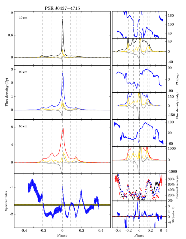
Figure 5: Multi-frequency polarization pulse profiles and phase-resolved results for PSR J0437$-$4715. Multiple overlapping components and complex polarization variations are shown across the pulse profile. The overall pulse width is more than $300^{\circ}$ in all three bands. The main peak has two components with the second component having a steeper spectrum and disappearing at high frequencies. The leading and trailing parts of the main peak have steeper spectral indices. However, the outer edges of the profile have flat spectra. We have tried different baseline duty cycles from 0.1 to 0.05 in our processing and found that the results we present here are not significantly affected. The profile features are consistent with the Murchison Widefield Array (MWA) observation at a frequency of 192 MHz, which shows that at low frequencies the central bright component is flanked by multiple outer components (Bhat et al., 2014). The PA curves vary dramatically across observing bands. While the orthogonal transition close to the main profile peak exists in all three bands, the previously reported non-orthogonal transition at 20 cm around phase $-0.23$ disappears in the other two bands (Yan et al., 2011a). We observed a probable orthogonal transition at 50 cm around phase 0.25, and non-orthogonal transitions at 50 cm around phase 0.3 and $-0.02$ and at 10 cm around phase 0.05. The phase-resolved spectral indices, fractional linear polarizations and apparent RMs vary dramatically across the profile. Close to phase zero, we observed step changes in the phase-resolved spectral index and apparent RM, which coincide with the change in the distribution of phase-resolved electric field magnitude observed by Osłowski et al. (2014).

Figure 6: Multi-frequency polarization pulse profiles and phase-resolved results for PSR J0613$-$0200. Our high S/N profiles provide more details in the PA curve compared to previous observations, and we show that the PA curves are complex and very different in three bands. At 20 cm, the discontinuous PA at the leading edge of the trailing component reported by Yan et al. (2011a) is not observed, and the PA curve seems to be continuous. The main pulse of the profile shows clear frequency evolution, and most significantly, the trailing peak has a very steep spectrum. The trailing peak splits into two peaks at low frequencies as previously observed by Stairs et al. (1999). From the high frequencies to low frequencies, the fractional linear polarization increases, and the trailing component becomes highly linearly polarized. At 50 cm, the circular polarization swaps sign compared to higher frequencies. The three main pulse components of the profile clearly have different apparent RMs.

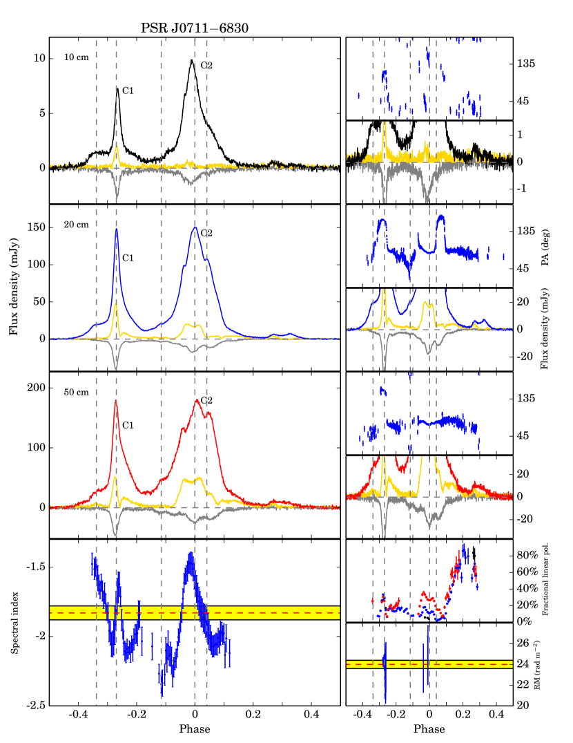
Figure 7: Multi-frequency polarization pulse profiles and phase-resolved results for PSR J0711$-$6830. The double-peaked weak component following the second peak is clear. The orthogonal mode transition after the peak of the leading component seen by Yan et al. (2011a) is confirmed at 20 cm and is seen at 50 cm. However the orthogonal mode transition near the trailing edge of the main peak is not present at 50 cm. The leading component has a slightly steeper spectrum than the main pulse. The fractional linear polarization of the main peak decreases significantly with increasing frequency.

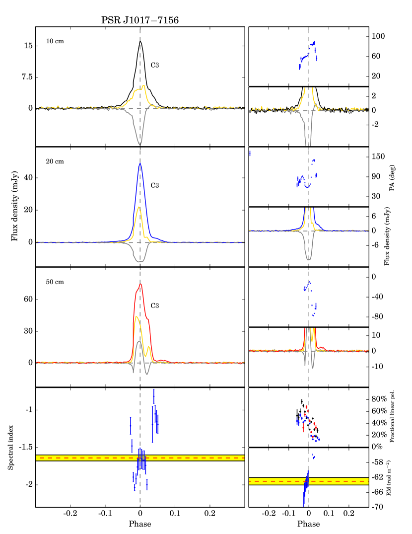
Figure 8: Multi-frequency polarization pulse profiles and phase-resolved results for PSR J1017$-$7156. We show that the PA variations are more complex than was observed in previous work. While the leading and trailing edges of the main pulse have a steeper spectrum compared with the central peak, the trailing component around phase 0.04 has a much flatter spectrum. Both the linear and circular polarization have multiple components and show significant evolution with frequency. Especially, the circular polarization of the main pulse seems to consist of two components of opposite sign with the left-circular component having narrower width and much steeper spectrum.

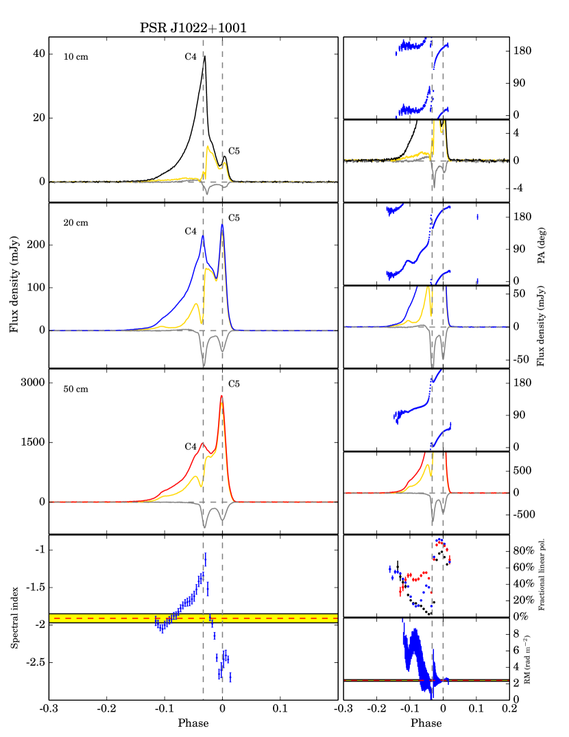
Figure 9: Multi-frequency polarization pulse profiles and phase-resolved results for PSR J1022$+$1001. At 10 cm, except for the discontinuity close to phase zero, the PA variation fits the RVM very well. As the frequency decreases, the PA variation departs from the RVM progressively. The spectral indices of two main peaks are significantly different so that the relative strength of the two main peaks evolves dramatically with frequency. While the second peak remains highly linearly polarized, the first peak depolarizes rapidly with increasing frequency. We also see systematic variation of the phase-resolved apparent RMs.

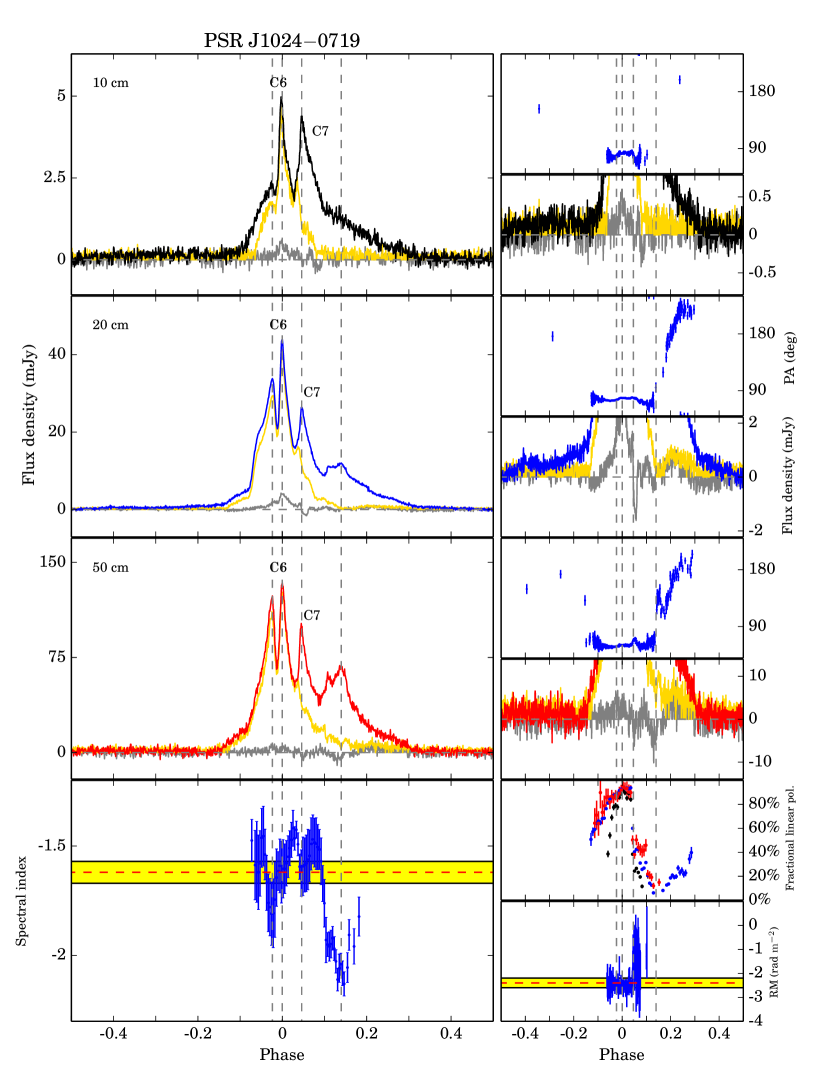
Figure 10: Multi-frequency polarization pulse profiles and phase-resolved results for PSR J1024$-$0719. Besides the flat PA curve across the main part of the profile as previously reported, we also show the PAs of the trailing component which increase with phase at 20 cm and 50 cm. The leading component and the trailing component of the profile have much steeper spectra compared with the central peaks. The leading part of the profile is highly linearly polarized and has stable phase-resolved RMs. As the fractional linear polarization drops down at the trailing part, the RMs show some variations.

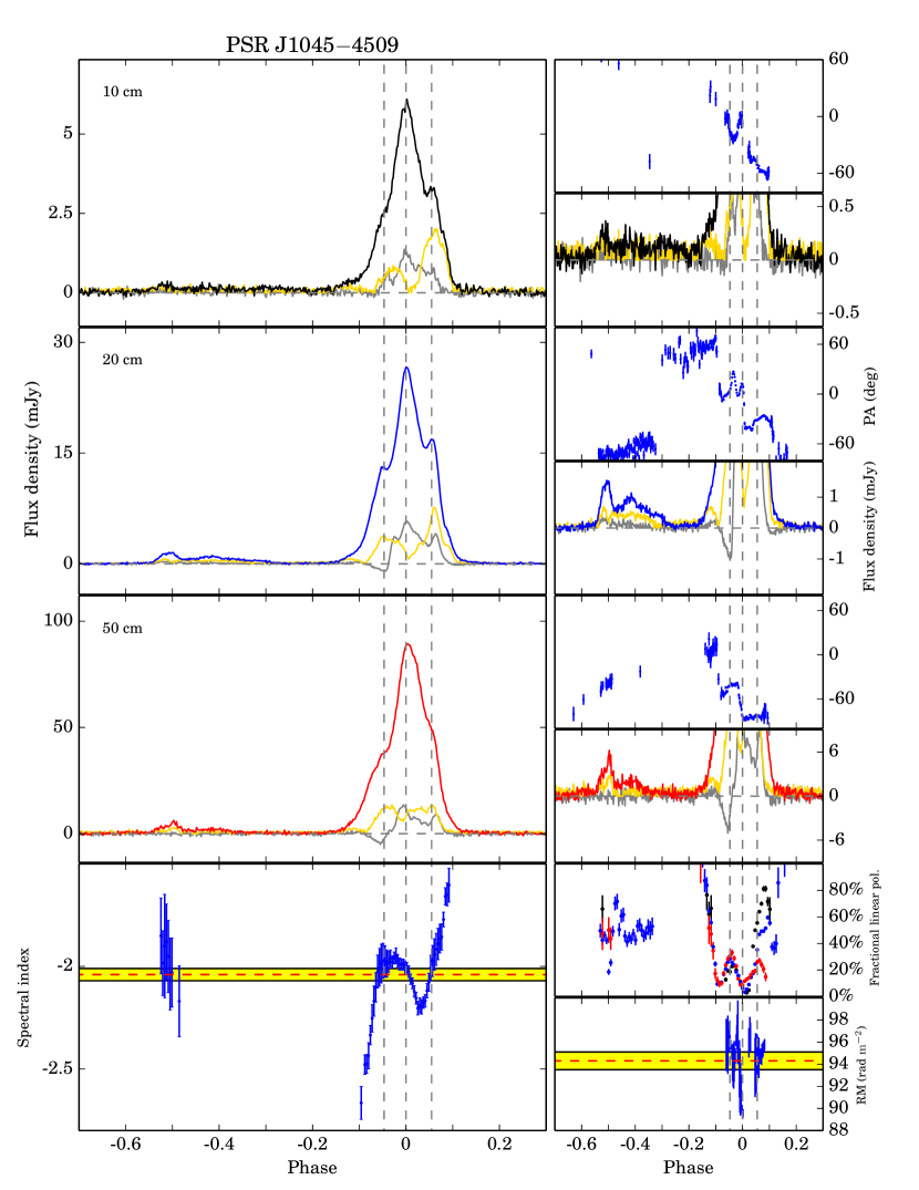
Figure 11: Multi-frequency polarization pulse profiles and phase-resolved results for PSR J1045$-$4509. We confirm that the leading emission is joined to the main pulse by a low-level bridge of emission as seen by Yan et al. (2011a). We show the complex PA curve with more detail, and determine the PA of the low-level bridge connecting the leading emission and the main pulse. At the leading edge of the main pulse, there is a non-orthogonal transition rather than an orthogonal transition as suggested by Yan et al. (2011a). Around phase zero, a non-orthogonal transition can be seen in all three bands. The PA of the low-level bridge emission seems to be discontinuous with the other PA variations and could be an orthogonal mode. To calculate the phase-resolved spectral index of the leading emission, we averaged the profile in frequency in the 10 cm band and only divided the 50 cm band into two subbands. We show that the leading edge of the main pulse has a steeper spectrum than that of the trailing edge. We also see an increase in the linear polarization of the trailing edge of the main pulse at high frequencies.

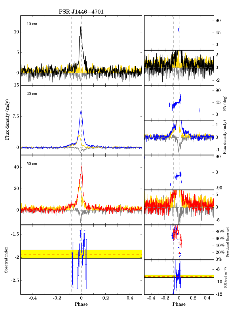
Figure 12: Multi-frequency polarization pulse profiles and phase-resolved results for PSR J1446$-$4701. The PAs are flat over the main pulse, but show variations over the leading and trailing parts. To calculate the phase-resolved spectral index, we averaged the profile in frequency in the 10 cm band and only divided the 50 cm band into two subbands. The linear polarization is much stronger at low frequencies.

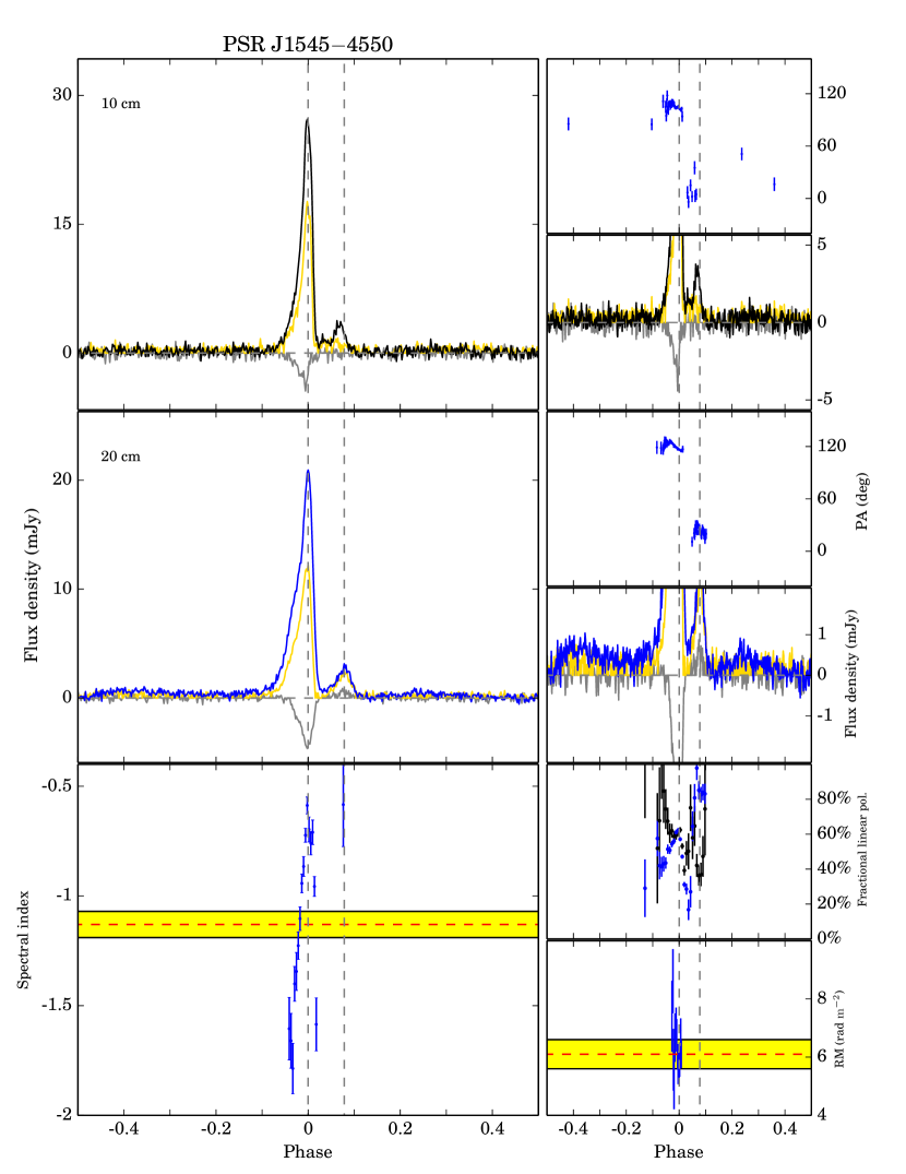
Figure 13: Multi-frequency polarization pulse profiles and phase-resolved results for PSR J1545$-$4550. At 20 cm, Burgay et al. (2013) show a component around phase $0.35$ that we do not see in our analysis. We have confirmed with the High Time Resolution Universe (HTRU) collaboration that this extra component resulted from an error in their analysis. At 10 cm, our results are consistent with those in Burgay et al. (2013). At 50 cm, we only have a few observations and the S/N is low, therefore we do not present the polarization profile here. We also show that low-level emission extends over at least $80$ per cent of the pulse period. There is an orthogonal transition between the main pulse and the trailing component.

Figure 14: Multi-frequency polarization pulse profiles and phase-resolved results for PSR J1600$-$3053. We show orthogonal transitions near the peaks of the two main components, which is consistent with previously published results. The leading component of the main pulse has a flatter spectrum compared with the main component. The central part of the pulse profile depolarizes rapidly with decreasing frequency. We see a sign swap of the circular polarization of the leading component from 20 cm to 10 cm, and at 50 cm, the circular polarization becomes almost zero across the whole profile.

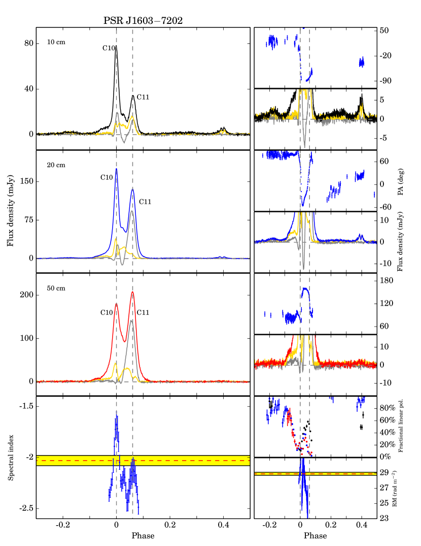
Figure 15: Multi-frequency polarization pulse profiles and phase-resolved results for PSR J1603$-$7202. The broad low-level feature preceding the main pulse and the double-peak trailing pulse can be clearly identified. We discovered new low-level emission connecting the main pulse and the double-peak trailing pulse, and it becomes stronger at 10 cm. The relative strength of the two main peaks evolves significantly with frequency. As frequency goes down, the second main peak becomes highly circularly polarized.

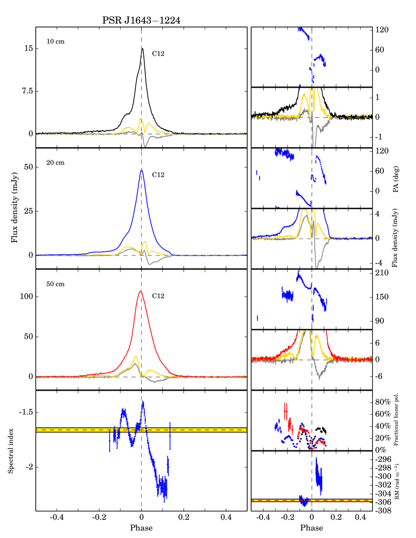
Figure 16: Multi-frequency polarization pulse profiles and phase-resolved results for PSR J1643$-$1224. At 10 cm and 20 cm, the PA of the broad feature preceding the main pulse is determined and found to be discontinuous with the rest of the PA variation, showing a new orthogonal transition. The main pulse clearly has multiple components and the trailing part has much steeper spectrum than other parts. The leading and trailing parts of the pulse have different apparent RMs.

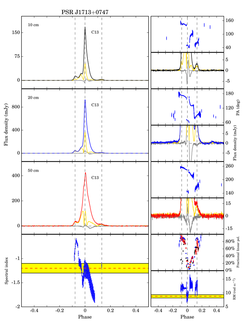
Figure 17: Multi-frequency polarization pulse profiles and phase-resolved results for PSR J1713$+$0747. At 20 cm and 50 cm, we show the almost complete linearly polarized leading and trailing components, which is consistent with previously published results. We detected weak emission around phase $-0.2$ and 0.35 at 20 cm, which increases the overall width from $104^{\circ}$ (as previously thought) to $199^{\circ}$. The non-orthogonal transition preceding the trailing pulse component reported by Yan et al. (2011a) is observed at 10 cm and 50 cm, but at 20 cm the PA transition is continuous. The linear polarization of the leading and trailing components become stronger at low frequencies relative to the rest of the profile. The main peak of the total intensity profile clearly has multiple components, and different components have different apparent RMs.

Figure 18: Multi-frequency polarization pulse profiles and phase-resolved results for PSR J1730$-$2304. We clearly show the weak leading and trailing components already reported, and at 20 cm we detect a weaker leading component not discovered before (around phase $-0.32$). This increases overall width of the pulse from $232^{\circ}$ to $248^{\circ}$. The pulse profile is very complex, with four clear peaks across the main pulse. To calculate the phase-resolved spectral index of the trailing component around phase 0.33, we averaged the profile in frequency in the 10 cm band and only divided the 50 cm band into two subbands. The central peak at 20 cm band has a steeper spectrum compared with other components. As the frequency goes down, the second peak depolarizes rapidly. The PA variations are very complex and are different in the three bands, leading to apparent RM variations across the profile.

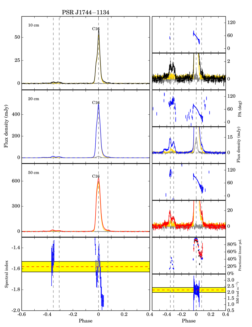
Figure 19: Multi-frequency polarization pulse profiles and phase-resolved results for PSR J1744$-$1134. The multiple-component precursor is clearly identified and no significant post-cursor component is observed. While the PAs of the main pulse show a smooth decrease, those of the precursor have clear structures and do not simply connect with the rest of the PA variations. The shape of the PA curves are similar in the three bands and the phase-resolved RMs are almost constant. The main pulse is highly linearly polarized from 10 cm to 50 cm. The circular polarizaion of main pulse grows stronger from 10 cm to 20 cm, but is weaker at 50 cm. To calculate the phase-resolved spectral index of the leading component around phase $-0.35$, we averaged the profile in frequency in the 10 cm band and only divided the 50 cm band into two subbands.

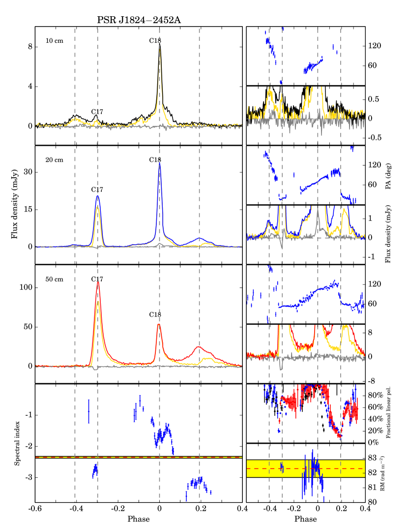
Figure 20: Multi-frequency polarization pulse profiles and phase-resolved results for PSR J1824$-$2452A. The weak component around phase $-0.4$ is clearly shown at 10 cm and 20 cm and is highly linearly polarized with a flat spectrum. We also show that there is low-level bridge emission connecting the two main components of the pulse profile. The PAs of preceding components are continuous themselves, but are discontinuous with the rest of the PA variations. To calculate the phase-resolved spectral index of the trailing component around phase 0.2, we averaged the profile in frequency in the 10 cm band. The frequency evolution of the total intensity is significant and our results are consistent with previous low frequency observations (e.g., Stairs et al., 1999). The phase-resolved spectral indices show huge variations related to the different components.

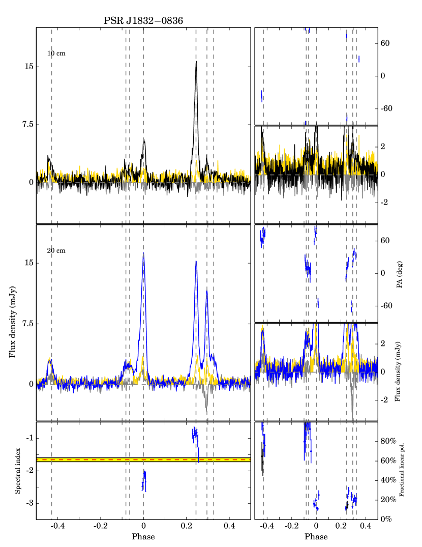
Figure 21: Multi-frequency polarization pulse profiles and phase-resolved results for PSR J1832$-$0836. At 50 cm, we only have a few observations and the S/N are low, therefore we do not present the polarization profile here. The components around phase $-0.45$ and $-0.08$ are highly linearly polarized and have relatively flat spectrum. The PAs around phase $-0.05$ and $0.3$ seem to be discontinuous, but is hard to confirm because of the low S/N.

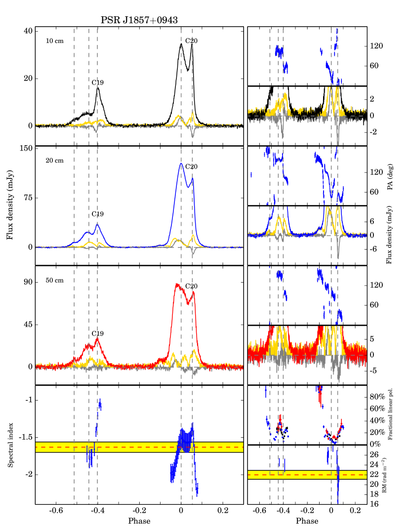
Figure 22: Multi-frequency polarization pulse profiles and phase-resolved results for PSR J1857$+$0943. We show more details of the PA variation, which is very complex and inconsistent with the RVM. At the leading edge of the main pulse, the PA decreases rapidly followed by an orthogonal mode transition. Around phase $0.05$, there is evidence of a non-orthogonal transition. Close to the peak of the interpulse, the PA shows a discontinuity at 20 cm, but becomes continuous at 10 cm. Both the main pulse and the interpulse have multiple components. The main peak of the interpulse has a relatively flat spectrum. The spectrum of the second peak of the main pulse is flatter than that of the first peak. The frequency development we observe is consistent with previous published results (Thorsett & Stinebring, 1990). At 50 cm there is a new linear polarization component appearing close to the center of the main pulse.

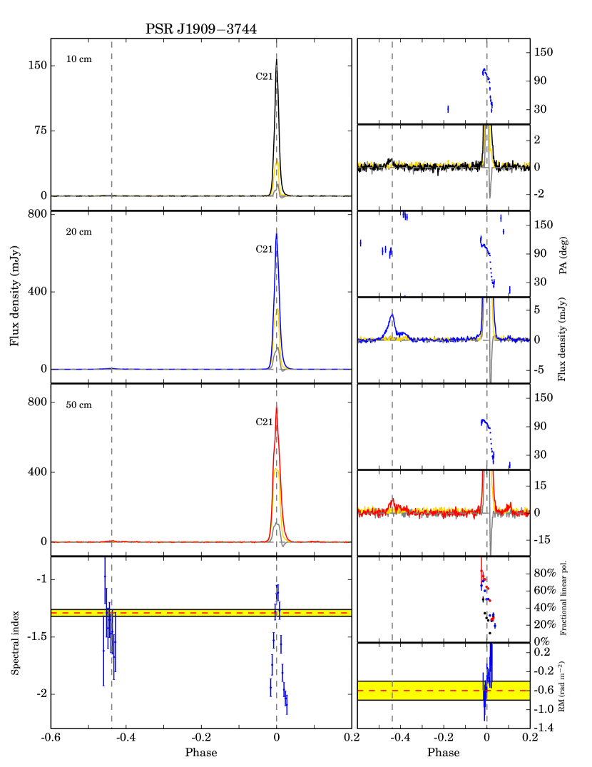
Figure 23: Multi-frequency polarization pulse profiles and phase-resolved results for PSR J1909$-$3744. We show a narrow main pulse and a weak feature preceding the main pulse by approximately $0.45$ in phase. There is little frequency evolution of the pulse profile, however, the fractional linear polarization increases as the frequency decreases. To calculate the phase-resolved spectral index of the leading component around phase $-0.45$, we averaged the profile in frequency in the 10 cm and 50 cm band.

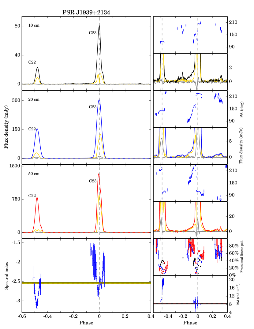
Figure 24: Multi-frequency polarization pulse profiles and phase-resolved results for PSR J1939$+$2134. Because of the high $\rm{DM}/P$, our observations are significantly affected by DM smearing, and we do not see the secondary maxima at the trailing edges of both the main pulses and interpulse  (Thorsett & Stinebring, 1990; Stairs et al., 1999; Ord et al., 2004). We confirm the existence of weak components preceding both the main pulse and interpulse seen by Yan et al. (2011a) and show that they are highly linearly polarized and stronger at 10 cm. Our results show stronger left-circular emission in the main pulse compared to Yan et al. (2011a). The interpulse has a steeper spectrum compared with the main pulse, and has a significantly different RM. The fractional linear polarization of the main pulse increases significantly as frequency decreases while that of the interpulse decreases.

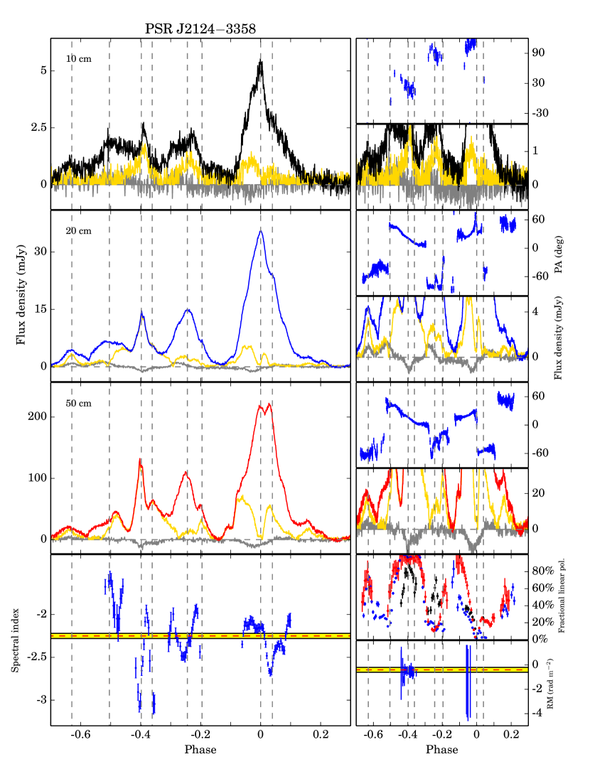
Figure 25: Multi-frequency polarization pulse profiles and phase-resolved results for PSR J2124$-$3358. We are able to provide more details of the PA variation and show that it has complex structures. At 20 cm, around phase $0.03$ and $-0.5$, there is evidence of two orthogonal mode transitions. At 50 cm, around phase $0.1$, there is a non-orthogonal transition of $\sim 110^{\circ}$. Because of the complexity of the profile, profile evolution is hard to describe. There are large variations of spectral index across the pulse longitude and these seem to be related to the different components, but this is complicated by the overlap of different components. We have tested that the phase-resolved spectral indices we present here are not significantly affected by the choice of baseline duty cycle and are generally consistent with those of Manchester & Han (2004). The fractional linear polarization of the main pulse increases at lower frequencies.

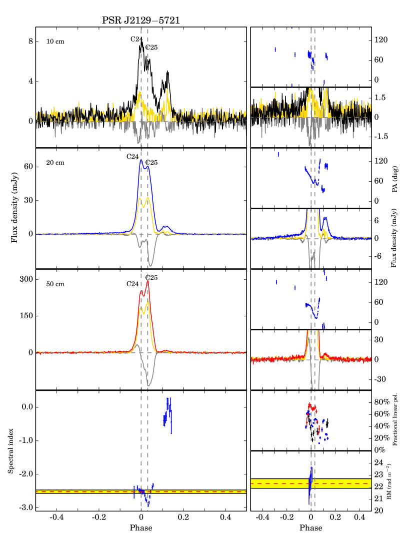
Figure 26: Multi-frequency polarization pulse profiles and phase-resolved results for PSR J2129$-$5721. At 20 cm, the weaker leading shelf of emission seen by Yan et al. (2011a) extends to at least phase of $-0.4$, and the post-cursor clearly has multiple components. We show more details of PA in the trailing edge of the main pulse. The PA decreases across the main pulse, and then increases quickly followed by an orthogonal mode transition at 20 cm. The post-cursor of the main pulse has much flatter spectrum. The fractional linear polarization of the main pulse increases as frequency decreases. To calculate the phase-resolved spectral index of the trailing component around phase 0.1, we averaged the profile in frequency in the 10 cm and 50 cm band. We show that the trailing component has a very flat spectrum.

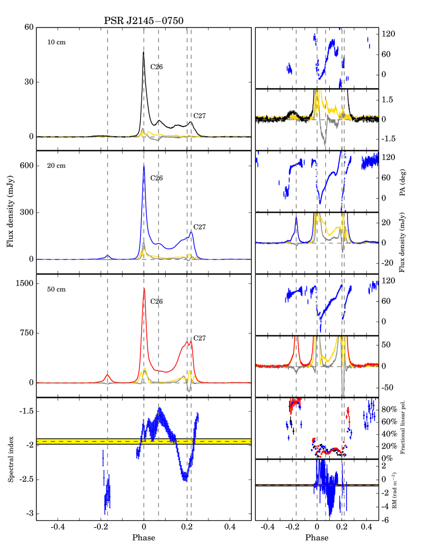
Figure 27: Multi-frequency polarization pulse profiles and phase-resolved results for PSR J2145$-$0750. At 20 cm, around phase $0.4$, there is evidence of new low-level emission which significantly extends the overall width of this MSP from $187^{\circ}$ to $277^{\circ}$. To calculate the phase-resolved spectral index of the leading component around phase $-0.18$, we averaged the profile in frequency in the 10 cm band. The trailing emission and the weak leading component have steeper spectra compared with other components.

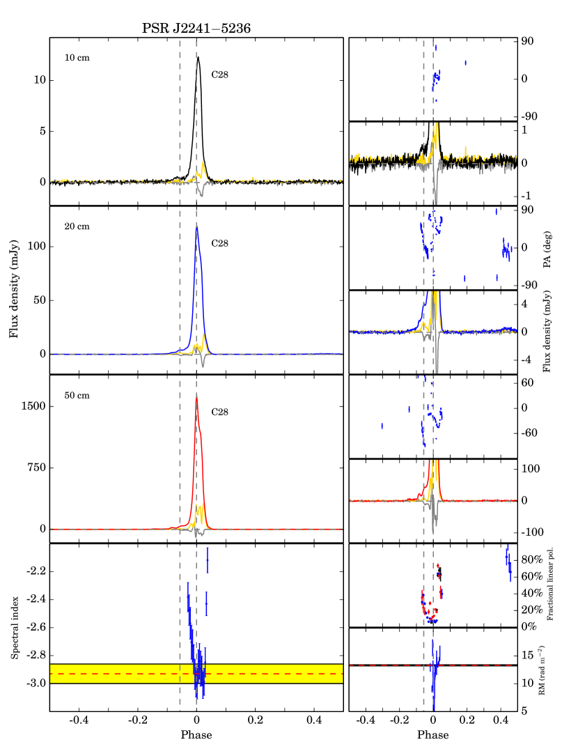
Figure 28: Multi-frequency polarization pulse profiles and phase-resolved results for PSR J2241$-$5236. At 20 cm, we show a new low-level component around phase $0.4$ with a width of approximately 0.2. We also show more details of the complex PA variations and there is evidence for two orthogonal mode transitions close to the peak. The frequency evolution of the pulse profile is hard to see, but the fractional linear polarization increases at lower frequencies.

References

- Abdo et al. (2009) Abdo A. A. et al., 2009, Science, 325, 848
- Abdo et al. (2010) Abdo A. A. et al., 2010, ApJS, 187, 460
- Abdo et al. (2013) Abdo A. A. et al., 2013, ApJS, 208, 17
- Barr et al. (2013) Barr E. D. et al., 2013, MNRAS, 429, 1633
- Basu et al. (2015) Basu R., Mitra D., Rankin J. M., 2015, ApJ, 798, 105
- Bhat et al. (2014) Bhat N. D. R. et al., 2014, ApJL, 791, L32
- Burgay et al. (2013) Burgay M. et al., 2013, MNRAS, 433, 259
- Chen & Wang (2014) Chen J. L., Wang H. G., 2014, ApJS, 215, 11
- Chen et al. (2007) Chen J.-L., Wang H.-G., Chen W.-H., Zhang H., Liu Y., 2007, ChJAA, 7, 789
- Cordes (1978) Cordes J. M., 1978, ApJ, 222, 1006
- Cordes & Shannon (2010) Cordes J. M., Shannon R. M., 2010, preprint (arXiv:1010.3785)
- Cordes & Shannon (2012) Cordes J. M., Shannon R. M., 2012, ApJ, 750, 89
- Crawford et al. (2000) Crawford F., Kaspi V. M., Bell J. F., 2000, Astron. J., 119, 2376
- Dyks & Rudak (2003) Dyks J., Rudak B., 2003, ApJ, 598, 1201
- Dyks et al. (2010) Dyks J., Rudak B., Demorest P., 2010, MNRAS, 401, 1781
- Espinoza et al. (2013) Espinoza C. M. et al., 2013, MNRAS, 430, 571
- Everett & Weisberg (2001) Everett J. E., Weisberg J. M., 2001, ApJ, 553, 341
- Foster & Backer (1990) Foster R. S., Backer D. C., 1990, ApJ, 361, 300
- Guillemot et al. (2012) Guillemot L. et al., 2012, ApJ, 744, 33
- Gupta & Gangadhara (2003) Gupta Y., Gangadhara R. T., 2003, ApJ, 584, 418
- Han & Manchester (2001) Han J. L., Manchester R. N., 2001, MNRAS, 320, L35
- Han et al. (2006) Han J. L., Manchester R. N., Lyne A. G., Qiao G. J., van Straten W., 2006, ApJ, 642, 868
- Hobbs et al. (2011) Hobbs G. et al., 2011, Publications of the Astronomical Society of Australia, 28, 202
- Hobbs et al. (2006) Hobbs G. B., Edwards R. T., Manchester R. N., 2006, MNRAS, 369, 655
- Hotan et al. (2004) Hotan A. W., van Straten W., Manchester R. N., 2004, Publications of the Astronomical Society of Australia, 21, 302
- Johnston et al. (1993) Johnston S. et al., 1993, Nature, 361, 613
- Johnston & Weisberg (2006) Johnston S., Weisberg J. M., 2006, MNRAS, 368, 1856
- Karastergiou (2009) Karastergiou A., 2009, MNRAS, 392, L60
- Karastergiou & Johnston (2007) Karastergiou A., Johnston S., 2007, MNRAS, 380, 1678
- Keith et al. (2013) Keith M. J. et al., 2013, MNRAS, 429, 2161
- Keith et al. (2012) Keith M. J. et al., 2012, MNRAS, 419, 1752
- Keith et al. (2011) Keith M. J. et al., 2011, MNRAS, 414, 1292
- Kennett & Melrose (1998) Kennett M., Melrose D., 1998, Publications of the Astronomical Society of Australia, 15, 211
- Kijak et al. (2011) Kijak J., Lewandowski W., Maron O., Gupta Y., Jessner A., 2011, A&A, 531, A16
- Kramer (1994) Kramer M., 1994, A&AS, 107, 527
- Kramer et al. (1999a) Kramer M., Lange C., Lorimer D. R., Backer D. C., Xilouris K. M., Jessner A., Wielebinski R., 1999a, ApJ, 526, 957
- Kramer et al. (1994) Kramer M., Wielebinski R., Jessner A., Gil J. A., Seiradakis J. H., 1994, A&AS, 107, 515
- Kramer et al. (1999b) Kramer M. et al., 1999b, ApJ, 520, 324
- Kramer et al. (1996) Kramer M., Xilouris K. M., Jessner A., Wielebinski R., Timofeev M., 1996, A&A, 306, 867
- Kramer et al. (1998) Kramer M., Xilouris K. M., Lorimer D. R., Doroshenko O., Jessner A., Wielebinski R., Wolszczan A., Camilo F., 1998, ApJ, 501, 270
- Kuzmin & Losovsky (2001) Kuzmin A. D., Losovsky B. Y., 2001, A&A, 368, 230
- Liu et al. (2014) Liu K. et al., 2014, MNRAS, 443, 3752
- Lorimer et al. (1995) Lorimer D. R., Yates J. A., Lyne A. G., Gould D. M., 1995, MNRAS, 273, 411
- Lyne & Manchester (1988) Lyne A. G., Manchester R. N., 1988, MNRAS, 234, 477
- Manchester (1995) Manchester R. N., 1995, Journal of Astrophysics and Astronomy, 16, 107
- Manchester (2005) Manchester R. N., 2005, Ap&SS, 297, 101
- Manchester & Han (2004) Manchester R. N., Han J. L., 2004, ApJ, 609, 354
- Manchester et al. (2013) Manchester R. N. et al., 2013, Publications of the Astronomical Society of Australia, 30, 17
- Manchester et al. (2005) Manchester R. N., Hobbs G. B., Teoh A., Hobbs M., 2005, Astron. J., 129, 1993
- Manchester & Johnston (1995) Manchester R. N., Johnston S., 1995, ApJL, 441, L65
- Maron et al. (2000) Maron O., Kijak J., Kramer M., Wielebinski R., 2000, A&AS, 147, 195
- Michel (1987) Michel F. C., 1987, ApJ, 322, 822
- Mitra & Li (2004) Mitra D., Li X. H., 2004, A&A, 421, 215
- Mitra & Rankin (2002) Mitra D., Rankin J. M., 2002, ApJ, 577, 322
- Navarro et al. (1997) Navarro J., Manchester R. N., Sandhu J. S., Kulkarni S. R., Bailes M., 1997, ApJ, 486, 1019
- Noutsos et al. (2009) Noutsos A., Karastergiou A., Kramer M., Johnston S., Stappers B. W., 2009, MNRAS, 396, 1559
- Ord et al. (2004) Ord S. M., van Straten W., Hotan A. W., Bailes M., 2004, MNRAS, 352, 804
- Osłowski et al. (2014) Osłowski S., van Straten W., Bailes M., Jameson A., Hobbs G., 2014, MNRAS, 441, 3148
- Pennucci et al. (2014) Pennucci T. T., Demorest P. B., Ransom S. M., 2014, ApJ, 790, 93
- Petrova (2002) Petrova S. A., 2002, A&A, 383, 1067
- Radhakrishnan & Cooke (1969) Radhakrishnan V., Cooke D. J., 1969, Astrophys. Lett., 3, 225
- Ramachandran et al. (2004) Ramachandran R., Backer D. C., Rankin J. M., Weisberg J. M., Devine K. E., 2004, ApJ, 606, 1167
- Rankin (1983) Rankin J. M., 1983, ApJ, 274, 333
- Ravi et al. (2010) Ravi V., Manchester R. N., Hobbs G., 2010, ApJL, 716, L85
- Shannon et al. (2014) Shannon R. M. et al., 2014, MNRAS, 443, 1463
- Shannon et al. (2013) Shannon R. M. et al., 2013, Science, 342, 334
- Stairs et al. (1999) Stairs I. H., Thorsett S. E., Camilo F., 1999, ApJS, 123, 627
- Taylor (1992) Taylor J. H., 1992, Royal Society of London Philosophical Transactions Series A, 341, 117
- Thorsett (1991) Thorsett S. E., 1991, ApJ, 377, 263
- Thorsett & Stinebring (1990) Thorsett S. E., Stinebring D. R., 1990, ApJ, 361, 644
- Toscano et al. (1998) Toscano M., Bailes M., Manchester R. N., Sandhu J. S., 1998, ApJ, 506, 863
- van Straten (2004) van Straten W., 2004, ApJS, 152, 129
- van Straten et al. (2010) van Straten W., Manchester R. N., Johnston S., Reynolds J. E., 2010, Publications of the Astronomical Society of Australia, 27, 104
- Wang et al. (2011) Wang C., Han J. L., Lai D., 2011, MNRAS, 417, 1183
- Wang et al. (2014) Wang H. G. et al., 2014, ApJ, 789, 73
- Wang et al. (2015) Wang J. B. et al., 2015, MNRAS, 446, 1657
- Wang et al. (2005) Wang N., Manchester R. N., Johnston S., Rickett B., Zhang J., Yusup A., Chen M., 2005, MNRAS, 358, 270
- Watters et al. (2009) Watters K. P., Romani R. W., Weltevrede P., Johnston S., 2009, ApJ, 695, 1289
- Xilouris et al. (1998) Xilouris K. M., Kramer M., Jessner A., von Hoensbroech A., Lorimer D., Wielebinski R., Wolszczan A., Camilo F., 1998, ApJ, 501, 286
- Yan et al. (2011a) Yan W. M. et al., 2011a, MNRAS, 414, 2087
- Yan et al. (2011b) Yan W. M. et al., 2011b, Ap&SS, 335, 485
- Zhu et al. (2014) Zhu X.-J. et al., 2014, MNRAS, 444, 3709