A Quantization Approach to the Counterparty Credit Exposure Estimation

Abstract

During recent years the counterparty risk subject has received a growing attention because of the so called Basel Accord. In particular the Basel III Accord asks the banks to fulfill finer conditions concerning counterparty credit exposures arising from banks’ derivatives, securities financing transactions, default and downgrade risks characterizing the Over The Counter (OTC) derivatives market, etc. Consequently the development of effective and more accurate measures of risk have been pushed, particularly focusing on the estimate of the future fair value of derivatives with respect to prescribed time horizon and fixed grid of time buckets . Standard methods used to treat the latter scenario are mainly based on ad hoc implementations of the classic Monte Carlo (MC) approach, which is characterized by a high computational time, strongly dependent on the number of considered assets. This is why many financial players moved to more enhanced Technologies, e.g., grid computing and Graphics Processing Units (GPUs) capabilities. In this paper we show how to implement the quantization technique, in order to accurately estimate both pricing and volatility values. Our approach is tested to produce effective results for the counterparty risk evaluation, with a big improvement concerning required time to run when compared to MC approach.

1 Introduction and scope of the study

The financial crisis in 2007-2008, along with a consequent increasing awareness about the different sources of risk, has suggested to the various financial players to give a greater attention to the counterparty credit risk (CCR). CCR refers to the situation when the counterparty A has a deal, mainly of derivative type, such as an option or a swap, subscribed with the counterparty B. We suppose that, according to a valuation criteria based on market prices, A observes a positive fair value, namely the so called Mark-to-Market (MtM). It follows that A has a credit exposure with B, hence, if B defaults and no future recovery rates or collateral was posted, then A loses exactly MtM, which is the cost for the replacement of the defaulted position. Such type of risk is of particular interest within the Over The Counter (OTC) derivatives markets, namely those markets which are characterized by having transactions settled directly between the two counterparties and outside the stock exchange.

A slightly different perspective of CCR needs to be taken into account when, in the risk management field, A wants to assess ex-ante the risk belonging to the financial position underwritten with B. In such a case, considering the possible default for B as a random event both in time and in its magnitude, it turns out that the current MtM is a rather rough measure of the credit exposure of A. A better approach is given by considering the Exposure At Default (EAD) parameter which can be seen as conservative expected value of the future MtM at the (random) default time. EAD parameter can be seen as conservative expected value of the future MtM at the default time. An official way to estimate the EAD in various contexts is given in the Basel framework, see [1], namely within the set of recommendations on banking laws and regulations issued by the Basel Committee on Banking Supervision. Such an approach is based on the Expected Positive Exposure (EPE) evaluation, namely on a prudent probabilistic time average of the future MtM. EAD follows just as a multiple, i.e. $EAD=\alpha\cdot EPE$.

Moreover, we recall that the international accounting standards require that in the derivatives evaluation a full fair value principle has to be satisfied, see, e.g., [15].

If the the counterparty solvency level falls, we observe a downgrade in its rating and/or an increase in its spread, therefore the related OTC balance sheet evaluation has to embody this effect. This implies that we have to adjust the MtM since it may decrease not only due to the usual market parameters, e.g. underlying price, underlying volatility, free risk rate, etc., but also because of the credit spread volatility.

We refer to such an MtM adjustment as Credit value Adjustment (CVA), and the related adjusted fair value is sometimes called the full fair value. The adjusted MtM will be denoted by $MtM^{A}$ and we have $MtM^{A}=MtM-CVA$.

Even if the derivative has not been closed, the CVA effect can cause a loss in the balance sheet, namely an unrealized loss. The Basel Committee estimates that $2/3$ of the losses in the financial crisis years in the OTC sector were unrealized losses in the evaluation process. The CVA (expected) loss is (or should be) absorbed by the balance sheet, while the CVA volatility must be faced by the regulatory capital. To this end, a new capital charge, the CVA charge, was introduced within the Basel III framework. We refer the reader to [14] for a skillful analysis of the accounting principles and to [2] for a detailed discussion about the capital charge.

The EAD and the CVA computations pose a lot of methodological, financial and numerical issues, as witnessed by a huge amount of literature developed so far, see, e.g., [9], for a detailed review.

The present paper aims at studying the feasibility and the trade off accuracy vs. computational effort of the quantization approach for the EAD-estimation (EPE), not at discussing the usefulness of EAD/CVA measures, nor the related underlying or volatility models, nor even at analyzing data quality and data availability. Therefore, our main goal is the numerical CCR analysis, while we will address the CVA issue in a future work.

In particular, we will consider a simple Black and Scholes model, without taking into consideration collateral parameters in order to focus the attention on the implemented numerical techniques.

The paper is organized as follows: Section 2 is a review of the EPE definition given by the Basel Committee, while in Section 3 we give a description of the quantization approach to the EPE with some theoretical results. Section 4 describes some practical cases and contains the set up of the associated numerical experiments, finally in Section 5 we report the obtained numerical results along with their interpretation.

2 The Basel EPE definition

In what follows we shall give a review about the Basel Committee guidelines concerning the estimation of the Exposure at Default, i.e. the EPE parameter. Let us set the following notations that will be used throughout the paper.

• Given a derivative maturity time $0<T<+\infty$, we consider $K\in\mathbb{N}^{+}$ time steps $0<t_{1}<t_{2}<\cdots<t_{K}$ which constitute the so called buckets array, denoted by ${\bf B}^{T,K}$, where usually, but not mandatory, $t_{K}=T$.

• For every $t_{k}\in{\bf B}^{T,K}$ we denote by $MtM\left(t_{k},S_{k}\right):=MtM\left(t_{k},S_{t_{k}}\right)$ the fair value (Mark-to-Market) of a derivative at time bucket $t_{k},$ with respect to the underlying value $S_{k},$ at time $t_{k}$.

  For the sake of simplicity, we denote by $t_{0}=0$ the starting time of the evaluation problem, by considering the European case.

• For every $t_{k}\in{\bf B}^{T,K}$ we denote by $MtM\left(t_{k},S^{k}\right):=MtM\left(t_{k},S^{t_{k}}\right)$ the fair value (Mark-to-Market) of a derivative at time bucket $t_{k}$, with respect to the whole sample path $S^{k}:=\left\{S_{t}:0\leq t\leq t_{k}\right\}$, with initial time $t_{0}=0$.

• Taking into account previous definitions, we indicate by $\varphi=\varphi\left(T-t_{k},S_{k},\Theta\right)$ the pricing function for the given derivative, where $\Theta$ represents the set of parameters from which such a pricing function may depends, e.g., the free risk rate $r$ or the volatility $\sigma.$

• We will use the notation $\phi^{MtM}$ to denote the Mark-to-Market value pricing function.

Remark 1.

We would like to underline that, in the Black-Scholes framework, the volatility surface has to be flat, which does not occur when real financial time series are considered. It follows that the above-mentioned pricing function $\phi$ most likely depends on more than the two considered parameters $r$ and $\sigma$. In particular, usually $\Theta\in\mathbb{R}^{n}$, with $n>2$, where the extra parameters characterize the specific geometric structure of the volatility surface associated to the considered contingent claim.

As usual in the counterparty credit risk EAD estimation, we stress the role of the underlying, understood as the only stochastic market parameter, while the others are deemed to be given, specifically, we assume that they are deterministic and constant or substituted by their deterministic forward values.

Henceforward, we shall often use the notation $\mathit{k}$ to indicate quantities of interest evaluated at the $k-$th time bucket $\mathrm{t_{k}}.$ Besides, we give an account of the main amounts that will be used in the following for EAD estimation, as they are defined in Basel III, [2].

• We denote the Expected Exposure (EE) of the derivative by

  $$EE_{k}:=\frac{1}{N}\sum_{n=1}^{N}MtM\left(t_{k},S_{k,n}\right)^{+},\;N\,\in\,\mathbb{N}^{+}\;,$$

  which is nothing but the arithmetic mean of $N$ Monte Carlo simulated MtM values, computed at the $k-$th time bucket $t_{k}$, with respect to the underlying $\mathrm{S}.$

  The positive part operator $\left(\cdot\right)^{+}$is effective if we are managing a symmetric derivative, such as an interest rate swap or a portfolio of derivatives. For a single option, it is redundant, as the fair value of the option is always positive from the buy side situation. We want to stress that the sell side does not imply counterparty risk, hence it is out of context.

• We evaluate the Expected Positive Exposure (EPE) by

  $$EPE:=\frac{\sum_{k=1}^{K}EE_{k}\cdot\Delta_{k}}{T},$$

  where $\Delta_{k}=t_{k}-t_{k-1}$ indicates the time space between two consecutive time buckets at $k$-th level. If the time buckets $t_{k}$ are equally spaced, then the formula reduces to $EPE=\frac{1}{K}{\sum_{k=1}^{K}EE_{k}}$. Therefore the EPE value gives the time average of the $EE_{k}.$

• We set

  $$EEE_{1}:=EE_{1}\mbox{ and }EEE_{k}:=Max\left\{EE_{k},EEE_{k-1}\right\}\;,\mbox{ for every }k=1,\ldots,K.$$

  Due to its non decreasing property, $EEE_{k},$ which is called the Effected Expected Exposure, takes into account the fact that, once the time decay effect reduces the MtM as well as the counterparty risk exposure, the bank applies a roll out with some new deals.

• We define the Effected Expected Positive Exposure (EEPE), by

  $$EEPE:=\frac{\sum_{k=1}^{K}EEE_{k}\cdot\Delta_{k}}{T}\;.$$

In order to avoid too many inessential regulatory details, we will work on $EE_{k}$ and EPE, the others being just arithmetic modifications of them.

Remark 2.

Let us point out that the definition of $EE_{k}$ is taken from the Basel regulatory framework. We find it quite strange, since, instead of giving a theoretical principle and suggesting the Monte Carlo technique just as a possible computational tool, the simulation approach is officially embedded in the general definition.

In what follows we shall rewrite previously defined quantities in continuous time, and we add the index $A$ to indicate the adjusted definitions. Moreover we consider the dynamics of the underlying $S_{t}:=\left\{S_{t}\right\}_{t\in[0,T]}$, $T\in\mathbb{R}^{+}$ being some expiration date, as an Itô processes, defined on some filtered probability space $\left(\Omega,\mathcal{F},\mathcal{F}_{t\in[0,T]},\mathbb{P}\right)$. As an example, $S_{t}$ is the solution of the stochastic differential equation defining the geometric Brownian motion, $\mathcal{F}_{t\in[0,T]}$ is the natural filtration generated by a standard Brownian motion $W_{t}=(W_{t})_{t\in[0,T]}$ starting from a complete probability space $\left(\Omega,\mathcal{F},\mathbb{P}\right)$, where $\mathbb{P}$ could be the so called real world probability measure or an equivalent risk neutral measure in a martingale approach to option pricing, see, e.g., [22, Ch.5].

The Adjusted Expected Exposure $EE^{A}$ is given by

$$EE_{k}^{A}:=\mathbb{E}_{\mathbb{P}}\left[MtM\left(t_{k},S_{k}\right)^{+}\right]=\int\varphi\left(t_{k},S_{k},\Theta\right)d\mathbf{\mathbb{P}}\cong\frac{1}{N}\sum_{n=1}^{N}MtM\left(t_{k},S_{k,n}\right)^{+}=\widehat{EE_{k}^{A}}$$ (1)

We define the Adjusted Expected Positive Exposure $EPE^{A}$ as

$$EPE^{A}:=\int EE_{t}^{A}\mathrm{d}t=\int\left[\int\varphi\left(t,S_{k},\Theta\right)\mathrm{d}\mathbb{P}\right]\mathrm{d}t\;.$$ (2)

In this new formulation, the Basel definition is simply one of the many methods to estimate the expected fair value of the derivative in the future.

Remark 3.

We skip any comment about the choice of the most suitable probability measure $\mathbf{\mathbb{P}}$ to be used in the calculation of $EE_{k},$ this being beyond the aim of this paper.

For a detailed discussion on the role played by the risk neutral probability for the drift $S_{t}$ or the historical real world probability, see, e.g., [8].

Remark 4.

Let us observe that the discount factor, or numeraire, is missing in the EPE definition. It was not forgot, but this is one of the several conservative proxies used in the risk regulation.

If we adopt a simulation approach, for the underlying path construction we could generate, for each simulation n, a path with an array of points $\left(x_{n,t_{k}}\right)$. This algorithm is called path-dependent simulation (PDS). Alternatively, for each time bucket and for each simulation, we could jointly generate our $N\cdot K$ points. This approach is referred as direct-jump to simulation date (DJS). We will come back on PDS and DJS approaches in Section 5.

The figures below, taken from [20], well clarify the difference

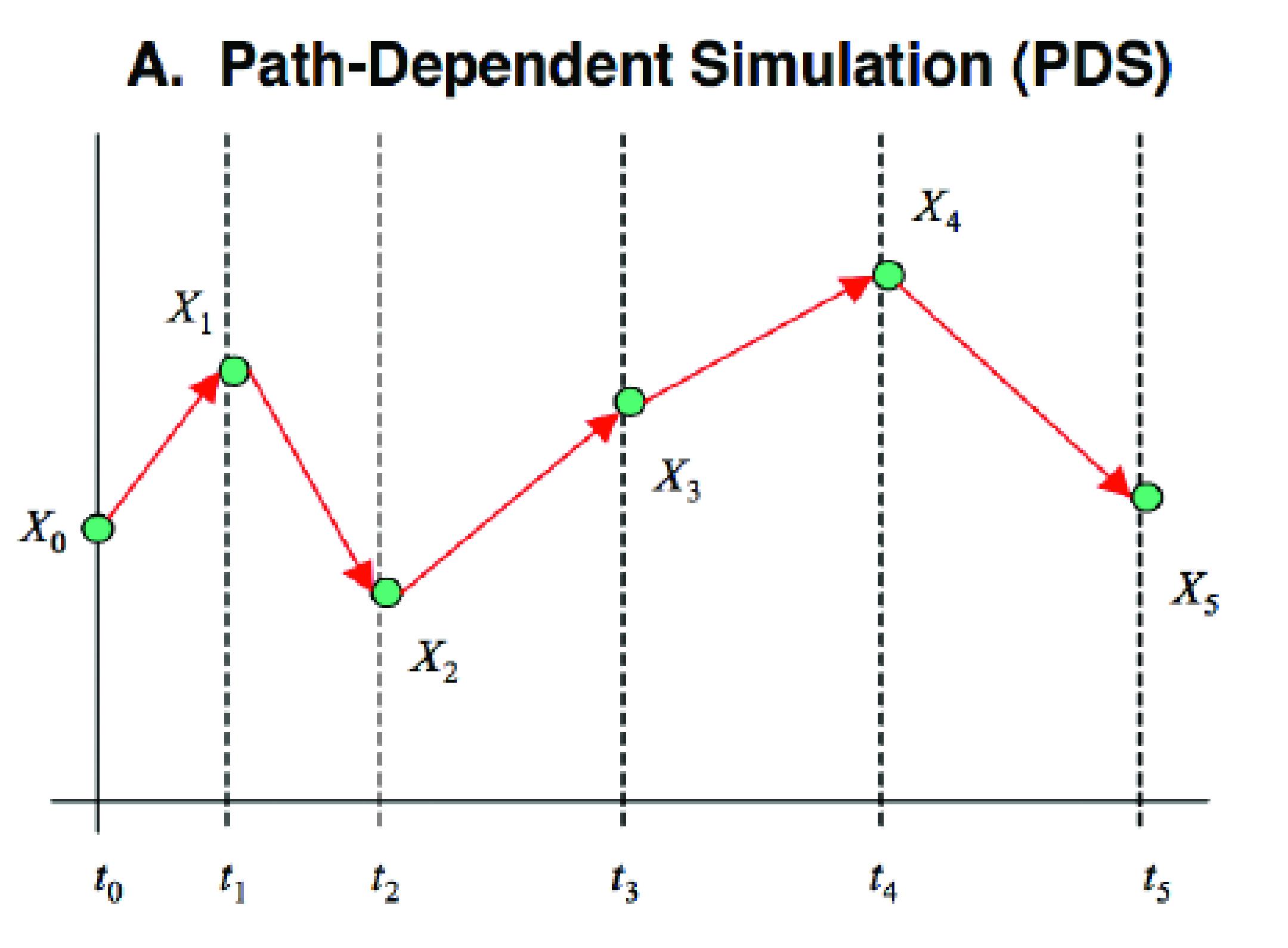
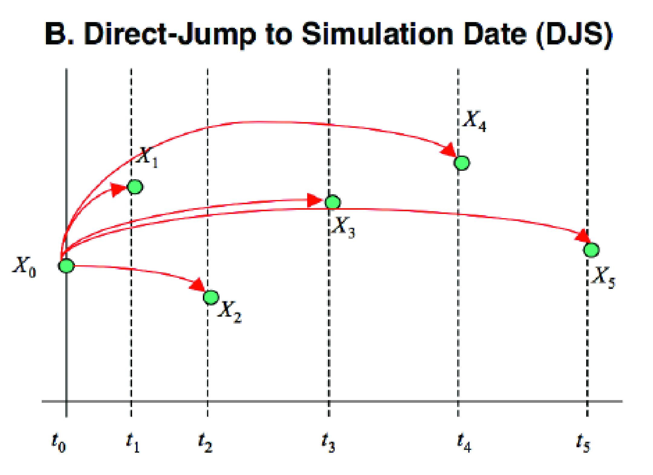
Figure 1: On the left: an example of PDS approach with six time buckets. On the right: an example of DJS approach with six time buckets.

Finally, we recall that, in the risk management application, another widely used quantity is the potential future exposure $PFE_{\alpha},$ a quantile based figure of the extreme risk. In a continuous setting, we define the potential future exposure in the following way

$$PFE\left(\alpha,t_{k}\right):=MtM^{*}\mbox{ such that }P\left\{MtM\left(t_{k},S_{k}\right)^{+}\geq MtM^{*}\right\}=1-\alpha\;.$$ (3)

3 A short quantization review

The quantization technique has been known from several decades and it comes from engineering, when addressing the issue of converting an analogical signal, e.g. images or sounds, into a discretized digital information. Other important areas of application are data compression and statistical multidimensional clustering. For a classical reference concerning the quantization approach, we refer to [11], while [16] gives a survey of the literature concerning fair value pricing problems for plain vanilla options, American and exotic options, basket CDS.

In addition, alternative quantization approaches, such as the so-called dual quantization and the treatment of underlying assets driven by more structured stochastic processes, are taken into consideration in [17] and [18].

In this section, we shall give a sketch of the quantization idea, by emphasizing its practical features, but without giving all the details concerning the mathematical theory behind it.

Let $X\in\mathbb{R}^{d}$, $d\in\mathbb{N}^{+}$, be a $d-$dimensional continuous random variable, defined over the probability space $\left(\Omega,\mathscr{\mathcal{F}},\mathbb{P}\right)$ and let $\mathbb{P}_{X}$ the measure induced by $X$. The quantization approach is based on the approximation of $X$ by a $d$-dimensional discrete random variable $\widehat{X}$, further details of which will be given later, defined by means of a so called quantization function $q$ of $X$, that is to say, $\widehat{X}:=q\left(X\right),$ in such a way that $\widehat{X}$ takes $N\in\mathbb{N}^{+}$ finitely many values in $\mathbb{R}^{d}.$ The finite set of values for $\widehat{X}$ is denoted by $q\left(\mathbb{R}\right):=\left\{x_{1},...,x_{N}\right\}$ and it is called a quantizer of $X,$ while the application $q\left(X\right)$ is the related quantization. To distinguish the one-dimensional case ($d=1$) from the $d-$dimensional one ($d>1$), the terms quantization, resp. vector quantization (VQ), are usually used.

Such a set of points in $\mathbb{R}^{d}$ can be used as generator points of a Voronoi tessellation. Let us recall that, if ${\bf{X}}$ is a metric space with a distance function ${\bf{d}},$ ${\bf{K}}$ is an index and $(P_{k})_{k\in{\bf{K}}}$ is a tuple of ordered collection of nonempty subsets of ${\bf{X}}$, then the Voronoi cell ${\bf{R}_{k}}$ generated by the site $P_{k}$ is defined as the following the set

$${\bf{R}}_{k}:=\left\{x\in X\;|\;{\bf d}(x,P_{k})\leq{\bf d}(x,P_{j})\;\text{for all}\;j\neq k\right\}\;.$$

Therefore, the Voronoi tessellation is the tuple of cells $\left({\bf R}_{k}\right)_{k\in{\bf{K}}}$. In our case such a tessellation reduces to substitute the set of cells $P_{k}$ with a finite number $x_{1},\ldots,x_{N}$ of distinct points in $\mathbb{R}^{d}$, so that the Voronoi cells are convex polytopes.

More precisely, we construct the following Voronoi tessels with respect to the euclidean norm $\|\cdot\|$ in $\mathbb{R}^{d}:$

$$C\left(x_{i}\right)=\left\{y\in\mathscr{\mathcal{\mathfrak{\mathbb{R^{\mathit{d}}}}\mathit{\mathrm{:}\left|y-x_{i}\right|<\|y-x_{j}\|\forall j\neq i}}}\right\}\;,$$

with associated quantization function $q$ defined as follows

$$q\left(X\right)=\sum_{i=1}^{N}x_{i}\cdot 1_{C_{i}\left(x\right)}\left(X\right)\;.$$ (4)

Such a construction allows us to rigorously define a probabilistic setting for the claimed random variable $\widehat{X},$ by exploiting the probability measure induced by the continuous random variable $X.$ In particular, we have a probability space $\left(\Omega,\mathcal{F},\mathbb{P}_{\widehat{X}}\right)$, where the set of elementary events is given by $\Omega:=\left\{x_{1},\ldots,x_{N}\right\}$, and the probability measure $\mathbb{P}_{\widehat{X}}$ is defined by the following set of relations

$$0<\mathbb{P}_{\widehat{X}}\left(x_{i}\right):=P_{X}\left(X\in C\left(x_{i}\right)\right)=:p_{i},\;\mbox{for }i=1,\ldots,N\;.$$

The goal of such an approximation is to deal efficiently with applications that arise when calculating some functionals of the random vector $X$, as in the derivative pricing problem case, in order to evaluate the expectation $\mathbb{E}\left[f\left(X\right)\right]$ of a certain payoff function $f$ of $X$ or when we have to deal with a quantile base indicator, as it happens in the risk management field.

We would like to take into account the former case, in particular we will consider the following approximation

$$\mathbb{E}\left[f\left(X\right)\right]\cong\mathbb{E}\left[f\left(\widehat{X}\right)\right]=\sum_{i}f\left(x_{i}\right)\cdot p_{i}\;,$$

with control on the accuracy of the chosen quantization.

Let us Assume $X\,\in\,L^{p}\left(\Omega,\mathrm{\mathscr{\mathcal{F}}},\mathbb{P}\right),p\,\in\,\left(1,\infty\right)$ and define the $L^{p}$ error as follows

$$E\left[\|X-\widehat{X}\|^{p}\right]:=\int_{\mathbb{R}^{d}}\mathrm{\min_{i=1,\ldots,N}}\|x-x_{i}\|^{p}\mathrm{d}\mathbb{P}_{X}\left(x\right)\;,$$ (5)

where we denote by $d\mathbb{P}_{X}$ the probability density function characterizing the random variable $X.$ The integrand in eq. (5) is always well defined, being a minimum with respect to the finite set of generators $x_{1},\ldots,x_{N}.$

Concerning eq. (5), the task is to find $the$, or, at least, one, optimal quantizer, understood as the set of Voronoi generators minimizing the value of the integral, once both parameters $d,N,p$ and the probability density of $X$ are given. Even if such a problem could be particularly difficult in the general case, also because it may rise to infinitely many solutions, this is not the case in our setting. In fact, we aim at considering a standard Black-Sholes framework, where the only source of randomness is given by a Brownian motion. In particular, we shall deal with the pricing problem related to a European style option, therefore we are interested in the distribution of the driving random perturbation at maturity time $T$, which means that we are dealing with the quest of an optimal quantizer for a $d$-dimensional Gaussian random variable, assumed to be standard, up to suitable transformation of coordinates, namely $X\sim\mathcal{N}\left(0,I_{d}\right)$.

Algorithms to get the optimal quantizer can be found within the aforementioned references. Moreover, when the dimension $d\leq 10,$ there is a well established literature concerning how to find the optimal quantizers when the Gaussian framework is considered, see, e.g., the web site http://www.quantize.maths-fi.com/ and [4, 16, 21].

A particularly important quantity related to the choice of the optimal quantizer is represented by the so called distortion parameter

$$D_{X}^{N}(\widehat{X}):=E\left[\|X-\widehat{X}\|^{2}\right]=\int_{\mathbb{R}^{d}}\mathrm{\min_{i=1,\ldots,N}}\|x-x_{i}\|^{2}\cdot d\mathbb{P}_{X}\left(x\right)\;,$$ (6)

which is defined with respect to the quantizer $\left\{x_{1},\ldots,x_{N}\right\}.$

If the quantization function $\widehat{X}$ takes values in the set of optimal generators, then the distortion parameter admits a minimum, which will be indicated by $\underline{D}_{X}^{N},$ with $lim_{N\rightarrow\infty}\underline{D}_{X}^{N}=0.$

The following theorem, originally due to Zador, see [23, 24], generalized by Bucklew and Wise in [6] and then revisited in [16] in its non asymptotic version as a reformulation of the Pierce lemma, gives a quantitative result about the distortion magnitude.

Theorem 5.

[Zador] Let $X\in L^{p+\varepsilon}\left(\Omega,\mathcal{F},\mathbb{P}\right)$, for $p\in(0,+\infty)$, $\varepsilon>0$, and let $\Gamma$ be the $N-$size tessellation of $\mathbb{R}^{d}$ related to the quantizer $\widehat{X}.$ Then,

$$\mathrm{\underset{\mathit{N}}{lim}}\left(N^{\frac{p}{d}}\mathrm{\underset{|\Gamma|\leq N}{\min}}\|X-\widehat{X}\|_{\mathbb{P}}^{p}\right)=J_{p,d}\left(\underset{\mathbb{R}^{d}}{\int}g^{\frac{d}{d+p}}\left(x\right)\mathrm{d}x\right)^{1+\frac{p}{d}}\;,$$ (7)

where we assume $\mathrm{d}\mathbb{P}=g\mathrm{d}\lambda_{d}+\mathrm{d}\nu,$ for some suitable function $g,$ and $\nu\perp\lambda_{d},$ $\mathrm{d}\lambda_{d}$ being the Lebesgue measure on $\mathbb{R}^{d}$, while the constant $J_{p,d}$ corresponds to the case $X\sim Unif\left([0,1]^{d}\right).$

Let us recall that the optimal quantizer is stationary in the sense that $E\left[X|\widehat{X}\right]=\widehat{X}$, hence $\int_{C\left(x_{i}\right)}\left(x_{i}^{*}-x\right)\mathrm{d}\mathbb{P}_{X}\left(x\right)=0,\>i=1,\ldots,N.$ In what follows, we focus on the case $d=1$ and $p=2,$ hence considering a one-dimensional stochastic process and the quadratic distortion measure, therefore, in terms of Th. (5), we have $J_{p,1}=\frac{1}{2^{p}\cdot\left(p+1\right)}$, hence $J_{2,1}=\frac{1}{12}.$

Remark 6.

For practical applications, and in order to compare numerical results obtained by quantization with those produced by standard Monte Carlo techniques, we are mainly interested in the order of convergence to zero of the distortion parameter. In particular, thanks to Zador Theorem, we have that the quadratic distortion is of order $O\left(N^{-2}\right).$

It is also possible to provide results concerning the accuracy of the approximation $\mathbb{E}\left[f\left(\widehat{X}\right)\right],$ by mean of the distortion’s properties, see [16]. In particular, we can distinguish the following cases:

Lipschitz case

if $f$ is assumed to be a Lipschitz function, then

$$\left|E\left[f\left(X\right)\right]-E\left[f\left(\widehat{X}\right)\right]\right|\leq K_{f}\cdot\left\|X-\widehat{X}\right\|_{1}\leq KL_{f}\cdot\left\|X-\widehat{X}\right\|_{2}\;.$$ (8)

The smoother Lipschitz derivative case

If $f$ is assumed to be continuously differentiable with Lipschitz continuous differential $Df$, then, by performing the quantization using an optical quadratic grid $\Gamma$ and by applying Taylor expansion, we have

$$\left|E\left[f\left(X\right)\right]-E\left[f\left(\widehat{X}\right)\right]\right|\leq KL_{Df}\cdot\left\|X-\widehat{X}\right\|_{1}\;.$$ (9)

The Convex Case

If $f$ is a convex function and $\widehat{X}$ is stationary, then exploiting the Jensen inequality, we have

$$E\left[f\left(\widehat{X}\right)\right]=E\left[f\left(E\left[X|\widehat{X}\right]\right)\right]\leq E\left[f\left(X\right)\right]\;,$$ (10)

hence, the approximation by the quantization is always a lower bound for the true value of $E\left[f\left(X\right)\right].$

Remark 7.

We emphasize that the (optimal) quantization grid for given parameter values of $N,d$ and $p$ is calculated off-line once and for all. Then, in the computational effort comparison vs. a strict sense Monte Carlo approach, we must take into account that with the quantization one only has to plug-in the points in the numerical model, not to calculate or simulate them.

Remark 8.

An increasing literature is devoted to the functional quantization. In this case, the “random variable”, which has to be discretized in an optimal way, belongs to a suited functional space, e.g. one can consider an application $X$ such that $X:\Omega\rightarrow\left(L_{T}^{2},\left\|\cdot\right\|_{2}\right),$ where $L_{T}^{2}=L_{T}^{2}\left(\left[0,T\right],\mathrm{d}t\right).$ We recall that, even if in mathematical finance applications the stochastic calculus in continuous time is a very useful tool, in practice we have to deal with discrete sampling, in fact, Asian options or any other look-back derivatives have to work with a discrete calendar for the fixing instants. Then, depending on the specific application, one can choose if to approximate the discrete time real-world-problem by optimal quantization or if it is better to quantize the continuous time setting and then to apply it to the practical application, see, e.g.,[17] for a survey on such a topic.

4 The Proposal: quantization for the EPE calculation

In the following, we focus our attention on the calculation of EPE for option styles derivatives in the Black-Scholes standard setting, see [5]. Strictly speaking, the underlying evolves according to the following stochastic differential equation

$$\mathrm{d}S_{t}=S_{t}\cdot\mathrm{d}t+\sigma S_{t}\mathrm{d}W_{t}\;,$$ (11)

with related solution

$$S_{t}=S_{0}\cdot\exp\left[\left(r-\frac{\sigma^{2}}{2}\right)t+\sigma W_{t}\right]\;,$$ (12)

where $r,\sigma>0,$ $(W_{t})_{t\geq 0}$ is a Brownian motion, while $S_{0}$ is the initial value of the underlying $S_{t}.$

It is well known that the plain vanilla call and put options have a closed pricing formula. Since we do not want to give here a survey on the several extensions to the model, we content ourselves saying that, in the equity and Forex derivatives markets, the most important model extensions of eq. (11) are the local volatility models, the Heston model and the SABR models, see, e.g., [10], [13], [12], respectively.

As usual in a new methodology proposal, as a first step we prefer to check the techniques in a simple framework, in order to have clear insights about its properties.

We guess that the Monte Carlo approach is just one of the many feasible techniques for EE and EPE calculation. After all, it is computationally quite expensive, as shown by the following example. A medium bank easily has $D=O\left(10^{4}\right)$ derivatives deals. In order to validate the internal models for the EPE calculation, usually the central banks require at least $K=20$ time steps and $N=2000$ simulations. Finally, let us suppose that the relevant underlying (often called risk factors) to be simulated have $O\left(10^{3}\right)$ order. It is the sum of equity underlying, FX significant rates and rate curve points. Let $U$ be such a parameter.

What about the computational effort for an EPE process task on the whole book? If we adopt a pure Monte Carlo strategy, we must distinguish between the two main steps:

1. simulation (and storage) of the underlying paths

2. evaluation of the EE quantities. We omit for simplicity the last EPE layer, since it is just an algebraic recombination of the EEs.

The first step implies a grid of $G=K\cdot N\cdot U=4\cdot 10^{7}$ points, which work as an input for the step 2. This one requires $NT=K\cdot N\cdot D=4\cdot 10^{8}$ different tasks. By recalling definition of $EE_{k},$ each of these tasks is a pricing process, which very often turns to be performed by a Monte Carlo algorithm with several thousands of simulation steps.

Generally speaking, the evaluation of EPE by rough Monte Carlo is $K\cdot N=O\left(10^{4}\right)$ more expensive than the usual daily end-of-day mark to market evaluation of the book.

Hence, we argue that the brutal Monte Carlo approach can not be a satisfactory way for the EPE calculation.

For this reason, some banks are exploiting some innovative technological approaches, such as the use of the graphical processing unit (GPU), instead of CPUs, to set up a parallel calculation system, with some new programming languages such as NVIDIA, while some other banks have been invested a lot buying grid computing platforms.

We believe that an algorithmic based improvement could be more efficient than the hardware innovation, or it can be combined with, and much less expensive. In the derivatives pricing field, such a mixed approach is well explained in [19].

Coming back to our credit exposure estimation, we try to figure how to use the quantization technique. At a first level, we can distinguish between path-dependent derivatives and non path-dependent derivatives, in the following pd and npd for brevity. We point out that this definition is different from the usual plain vs. exotic derivatives. Among the non path-dependent derivatives we include not only the plain European options, but also European and American style options with exotic payoff, e.g. mixed digital continuous, spread options, etc. In the npd class, we will work with the Asian options, probably the most popular one.

For the npd derivatives, the quantization for the EPE simply reduces to set up the problem by selecting the parameters $\left(N_{k}\right)_{k=1,\ldots,K}$ for the quantization size at each time bucket $\left(t_{k}\right)$ and then to compute the EPE quantized approximation. We use the optimal quantizer case, recalling that

$$S_{0}\exp\left[\left(r-\frac{\sigma^{2}}{2}\right)t+\sigma\cdot W_{t}\right]=S_{0}\exp\left[\left(r-\frac{\sigma^{2}}{2}\right)t+\sigma\cdot\sqrt{t}\cdot N\left(0,1\right)\right]\;.$$

More formally, if we indicate by the exponent Q the quantized EPE, one easily gets

$$EE_{k}^{Q} =\sum_{i=1}^{N_{k}}MtM\left(t_{k},S\left(x_{i}^{k}\right)\right)^{+}p_{i}^{k}\;,$$ (13)

$$EPE^{Q} =\frac{\sum EE_{k}^{Q}\cdot\Delta_{k}}{T}=\frac{\underset{k}{\sum}\Delta_{k}\left(\sum_{i=1}^{N_{k}}MtM\left(t_{k},S\left(x_{i}^{k}\right)\right)^{+}\cdot p_{i}^{k}\right)}{T}\;.$$ (14)

Fig. (2), graphically explains the calculation procedure. In particular, the black point on the left is the underlying level at time $t_{0}$. For each time step $t_{k}$ and for each point of the quantizer $x_{i}^{k}$, a MtM is calculated and it is weighted by the probability $p_{i}^{k}.$ Hence $EE^{Q}$ and $EPE^{Q}$ straightly follow.

Figure 2: evolution of $EE^{Q}$ at every time bucket $t_{k}.$

Concerning the theoretical properties of such an approximation, we provide a useful result, which can be easily applied to the case of European style options.

Proposition 9.

Let us consider an option in the Black and Scholes setting, with $d=1$ and suppose that the pricing function $\varphi\left(\cdot\right)$ is Lipschitz continuous or continuously differentiable with a Lipschitz continuous differential.

Moreover, let us define $D_{N}^{EPE}:=\left|EPE^{A}-EPE^{Q}\right|^{2},$ where $EPE^{A}$ is the Adjusted Expected Positive Exposure, defined in eq. (2), and $EPE^{Q}$ is the quantized Expected Positive Exposure, defined in eq. (14). Then, we have

$$D_{N}^{EPE} \propto N^{-2}\cdot K^{-1},\mbox{ if $\varphi$Lipschitz continuous}\;,$$

$$D_{N}^{EPE} \propto N^{-4}\cdot K^{-1},\mbox{ if $\varphi$cont. differentiable with Lipschitz cont. differential}\;.$$

Proof.

By definition, we have

$$\left|EPE^{A}-EPE^{Q}\right|^{2}=\left|\frac{\sum EE_{k}^{A}\Delta_{k}}{T}-\frac{\sum EE_{k}^{Q}\Delta_{k}}{T}\right|^{2}=\frac{1}{T^{2}}\left|\sum\Delta_{k}\cdot\left(EE_{k}^{A}-EE_{k}^{Q}\right)\right|^{2}\;,$$

hence rearranging the terms and recalling that the CCR is effective just for the buy side position, we can skip the positive part obtaining

$$\left|\sum\Delta_{k}\left(EE_{k}^{A}-EE_{k}^{Q}\right)\right|^{2} =\left|\sum\Delta_{k}\cdot\left(\mathbf{E}_{\mathbf{P}}\left[MtM\left(t_{k},S_{k}\right)\right]-\mathbf{E}_{\mathbf{\widehat{P}}}\left[MtM\left(t_{k},S_{k}\right)\right]\right)\right|^{2}$$

$$\leq\sum\Delta_{k}^{2}\left(\mathbf{E}_{\mathbf{P}}\left[MtM\left(t_{k},S_{k}\right)\right]-\mathbf{E}_{\mathbf{\widehat{P}}}\left[MtM\left(t_{k},S_{k}\right)\right]\right)^{2}\;.$$ (15)

Moreover, we have

$$\left|\sum\Delta_{k}\left(EE_{k}^{A}-EE_{k}^{Q}\right)\right|^{2}\leq\left(\sum\Delta_{k}\left|\mathbf{E}_{\mathbf{P}}\left[MtM\left(t_{k},S_{k}\right)\right]-\mathbf{E}_{\mathbf{\widehat{P}}}\left[MtM\left(t_{k},S_{k}\right)\right]\right|\right)^{2}\;.$$

In a more explicit fashion, let us work on the single element $k$ of the summation, i.e. $\left(\mathbf{E}_{\mathbf{P}}\left[MtM\left(t_{k},S_{k}\right)\right]-\mathbf{E}_{\mathbf{\widehat{P}}}\left[MtM\left(t_{k},S_{k}\right)\right]\right).$ If we consider $MtM\left(t_{k},S_{k}\right)=\varphi\left(t_{k},S_{k}\left(X\right)\right)$ as the function appearing in eq. (8) and eq. (9), we get, respectively,

$$\left(\mathbf{E}_{\mathbf{P}}\left[MtM\left(t_{k},S_{k}\right)\right]-\mathbf{E}_{\mathbf{\widehat{P}}}\left[MtM\left(t_{k},S_{k}\right)\right]\right)^{2} \leq KL_{f,k}^{2}\cdot\left\|X_{k}-\widehat{X_{k}}\right\|_{1}^{2}$$ (16)

$$\left|\mathbf{E}_{\mathbf{P}}\left[MtM\left(t_{k},S_{k}\right)\right]-\mathbf{E}_{\mathbf{\widehat{P}}}\left[MtM\left(t_{k},S_{k}\right)\right]\right| \leq KL_{Df,k}^{2}\cdot\left\|X_{k}-\widehat{X_{k}}\right\|_{2}^{2}\;.$$ (17)

By replacing eq. (16) and eq. (17) in eq. (15), we obtain

$$\left|\sum\Delta_{k}\left(EE_{k}^{A}-EE_{k}^{Q}\right)\right|^{2} \leq\sum\Delta_{k}^{2}KL_{f,k}^{2}\cdot\left\|X_{k}-\widehat{X_{k}}\right\|_{1}^{2}\;,$$ (18)

$$\left|\sum\Delta_{k}\left(EE_{k}^{A}-EE_{k}^{Q}\right)\right|^{2} \leq\sum\Delta_{k}^{2}KL_{Df,k}^{2}\cdot\left\|X_{k}-\widehat{X_{k}}\right\|_{2}^{4}\;.$$ (19)

Let us consider eq. (18), the calculation for eq. (19) being the same.

Set $\overline{KL}$ equal to the mean of $\left(KL_{\cdot,k}\right),$ for all $k,$ and suppose that the mesh $t_{k}$ is regular enough, i.e. we require that $\mathrm{lim_{K}}\Delta_{k}=0,\,O\left(\Delta_{k}\right)=K^{-1}\;\forall\,k.$ Thanks to the Zador Theorem and taking $N\rightarrow+\infty$, we have

$$\frac{1}{T^{2}}\cdot\left|\sum\Delta_{k}\left(EE_{k}^{A}-EE_{k}^{Q}\right)\right|^{2} \leq\frac{1}{T^{2}}\sum\Delta_{k}^{2}KL_{f,k}^{2}\left\|X_{k}-\widehat{X_{k}}\right\|_{2}^{2}$$

$$\propto\frac{1}{T^{2}}\cdot K\cdot\overline{KL}\cdot\frac{T^{2}}{K^{2}}\cdot N^{-2}\;.$$

By simplifying, we get the result. Similar calculations provide the result when the pricing function is assumed to be continuously differentiable with Lipschitz continuous differential. For a more abstract setting, see [16, Sec.2.4]. ∎

Remark 10.

Let us discuss the hypothesis under which the result holds. The central role is played by the function $\varphi\left(x,\cdot\right)$ as a function of the Brownian motion $W_{t}$, that is, of the quantity $x\cdot\sqrt{t}$, $x$ sampled from the $N\left(0,1\right).$ We recall in fact that the usefulness of the quantization is to infer the properties of the approximation in the specific problem, starting from the Gaussian optimized discretization. As an example, for a put option the pricing function is bounded, Lipschitz continuous and twice differentiable, since the Black-Scholes formula is $C^{\infty}.$ Then, the above proposition holds.

For a call style option, the convexity properties easily holds, hence the quantization gives us a lower bound to the EPE estimation.

Remark 11.

If we consider the pricing function $\varphi\left(\cdot\right)$ as the elementary unit of our EPE computational work-flow, the computational complexity of the quantized approach is $\underset{k}{\sum N_{k}},$ to be compared with the global number of Monte Carlo scenarios simulations.

For path-dependent derivatives, for each time $t_{k},$ at least in a discrete sampling sense, one needs the whole path of the underlying. Hence, the above approach is not satisfactory, as the pricing function depends not only on the current level $S_{k},$ but also on some functions, e.g. the average, min, max, etc., of the underlying level until $t_{k}$. Latter task can be efficiently studied by an approach like the PDS one, as in figure 1.

Let $N_{k}$ be a positive integer for the quantization, and $q_{k}\left(\mathcal{R}\right)=\left(x_{1},x_{2,}...,x_{N_{k}}\right)$ is the quantizer of size $N_{k},$ namely the random variable $\widehat{X_{k}}=q\left(X_{k}\right)$ that maps the random variable to an optimal discrete version. If we refer to the Black-Scholes model, we want to quantize at each step the Brownian motion $W_{t}$ that generates the log-normal underlying process. We recall that $W_{t}\sim N\left(0,t\right)$ is a normal centered random variable and that $W_{t}-W_{s}\sim N\left(0,t-s\right).$

Again, we define $C\left(x_{i}\right)$ as the $i-$th Voronoi tessel such that

$$C\left(x_{i}\right):=\left\{y\in\mathscr{\mathcal{\mathfrak{\mathbb{R^{\mathit{d}}}}\mathit{\mathrm{:}\left|y-x_{i}\right|<\left|y-x_{j}\right|\forall j\neq i}}}\right\},$$

with the so-called nearest neighborhood principle. A set of probability masses vectors is assigned to the $N_{k}-$tuple, let be $\mathbf{p^{k}}=\left(p_{1}^{k},p_{2}^{k},\ldots,p_{N_{k}}^{k}\right),$ where $p_{i}=\mathbb{P}\left(C\left(x_{i}\right)\right)$ under the original probability $\mathcal{\mathbb{P_{X}}},$ for all $i=1,\ldots,N_{k}.$ The following questions naturally arise: how and where to use the quantizers for the $EE_{k}$ calculation ? The quantization tree is a discrete space, discrete time process, defined by

$$p_{i}^{k} =\mathbf{\mathbb{P}\mathrm{\left(\mathit{\widehat{X}_{k}}=x_{i}^{k}\right)}}=\mathbb{P}\left(X_{k}\in C_{i}\left(x^{k}\right)\right)\;,$$ (20)

$$\pi_{ij}^{k} =P\left(\widehat{X}_{k+1}=x_{j}^{k+1}|\widehat{X}_{k}=x_{i}^{k}\right)=P\left(X_{k+1}\in C_{j}\left(x^{k+1}\right)|X_{k}\in C_{i}\left(x^{k}\right)\right)$$

$$=\frac{P\left(X_{k+1}\in C_{j}\left(x^{k+1}\right),X_{k}\in C_{i}\left(x^{k}\right)\right)}{p_{i}^{k}}$$ (21)

The following theoretical result allows us to explicitly solve the transition probability formula (4), by recalling that $X_{k}$ is the original Brownian motion sampled at a given time $t_{k}.$

Proposition 12.

Let us use denote by $\Delta_{k}:=t_{k+1}-t_{k}$ the time space between two consecutive time buckets and by $\phi$ the density of the $N\left(0,1\right)$ random variable. Furthermore, let us indicate by $U_{k},U_{k+1}$, resp. by $L_{k},L_{k+1}$, the upper, resp. lower, bounds of the $1-$dimensional tessels $C_{i}\left(x^{k}\right)$ and $C_{j}\left(x^{k+1}\right).$

Then, the transition probability $\pi_{ij}^{k}$ assumes the following expression

$$\pi_{ij}^{k}=\int_{C_{j,k+1}}f\left(x_{k+1}|C_{i,k}\right)\mathrm{d}x_{k}=\frac{\intop_{L_{k}}^{U_{k}}\left(\intop_{L_{k+1}}^{U_{k+1}}\phi\left(\frac{\left(x-y\right)}{\sqrt{\Delta_{k}}}\right)\mathrm{d}x\right)\phi\left(\frac{y}{\sqrt{t_{k}}}\right)\cdot dy}{p_{i}^{k}}\;.$$ (22)

Proof.

The result is a straightforward calculation, indeed let us start considering a more specific problem, namely we aim at calculate $P\left(X_{k+1}\in C_{j}\left(x^{k+1}\right)|X_{k}=y,\>y\in C\left(x^{k}\right)\right).$

For given $x\in C_{j}\left(x^{k+1}\right)$, $y\in C_{j}\left(x^{k}\right)$, by recalling the scaling property and the independence of the Brownian motion increments, we easily get $P\left(\mathrm{d}x\right)=\phi\left(\frac{\left(x-y\right)}{\sqrt{\Delta}_{k}}\right)\cdot\mathrm{d}x$, and the result follows by extending such a fact to tessels $C_{i},C_{j}$.∎

The picture below shows the practical features of the formula eq. (22).

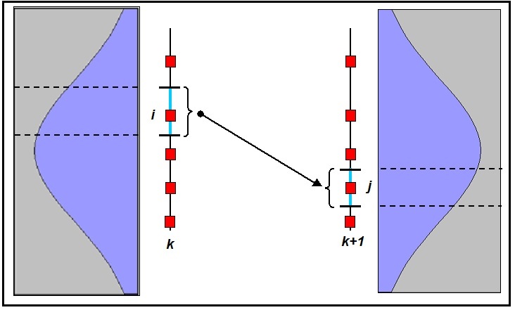
Figure 3: a graphical representation of the transition probability function

Remark 13.

Even if the proposition comes from elementary probability, this result is a useful improvement to the procedure in Pagès et al (2009), where a Monte Carlo approach for the $\pi_{ij}^{k}$ was suggested.

Remark 14.

From a computational complexity point of view, we observe that the above coefficients $\pi_{ij}^{k}$ can be calculated off line, once and for all, given the time discretization parameter $K$ and the chosen granularities $\left\{N_{1},N_{2},...,N_{K}\right\}.$

Despite the reduction in the number of evaluations that the quantization approach guarantees, the possible paths of the quantization tree, say $NP,$ could be too many from a theoretical perspective. In fact, they amount to $NP=\prod_{k}N_{k}$. If we set, as usual, $K=O\left(10^{1}\right)$ and $N_{k}=O\left(10^{2}\right),$ then $NP=O\left(10^{20}\right),$ which seems to be intractable for practical purposes. Fortunately, this does not occur, from a practical point of view. Many paths have a negligible probability, as very often we have $\pi_{ij}^{k}\simeq 0,$ so we can skip a large fraction of the combinatorial cases by some heuristic a priori rule that avoids calculation depending from the distance $\left|\left(\frac{x_{j}^{k+1}-x_{i}^{k}}{\sqrt{\varDelta_{k}}}\right)\right|$.

5 The numerical Application

In this section we will give an application of quantization method in CCR with respect to a portfolio consisting of a bank account and one risky asset which is the underlying of a European type option. We suppose that the dynamics of the underlying $S_{t}:=\left\{S_{t}\right\}_{t\in[0,T]}$, for some maturity time $T\in\mathbb{R}^{+}$, is given accordingly to a geometric Brownian motion, namely

$$\mathrm{d}S_{t}=rS_{t}\mathrm{d}t+\sigma S_{t}\mathrm{d}W_{t}\;,$$ (23)

where $r$ is the risk free interest rate, e.g. associated to a bank account, $\sigma$ is the volatility parameter characterizing the underlying behaviour, while $W_{t}:=\{W_{t}\}_{t\,\in\,[0,T]}$ is a $\mathbb{R}-$ valued Brownian motion on the filtered probability space $\left(\Omega,\mathcal{F},\mathcal{F}_{t},\mathbb{P}\right)$, $\left\{\mathcal{F}_{t}\right\}_{t\in[0,T]}$ being the filtration generated by $W_{t}$. We recall that the stochastic differential equation (23) admits an explicit solution, see, e.g.,[22, Ch.3], given by

$$S_{t}=S_{0}\exp\left\{\sigma W_{t}+\left(r-\frac{\sigma^{2}}{2}\right)t\right\}\;,$$ (24)

$S_{0}$ being the initial value of the underlying $S_{t}$.

If we consider a European call option with strike price $K\in\mathbb{R}^{+}$ snd maturity time $T$, written on $S_{t}$ described as above, then its fair value $C_{eu}=C_{eu}(S_{0},r,K,\sigma,T)$, with respect to the unique martingale equivalent measure, is given by

$$C_{eu}(S_{0},r,K,\sigma,T) :=e^{-rT}\mathbb{E}\left[\left(S_{T}-K\right)^{+}\right]$$

$$=e^{-rT}\mathbb{E}\left[\left(S_{0}\exp\left\{\left(r-\frac{\sigma^{2}}{2}\right)T+\sigma W_{T}\right\}-K\right)^{+}\right]\;,$$ (25)

with explicit solution given by the Black-Scholes formula.

Before enter into details about a numerical application of our proposal, see Sec. (4), to a concrete case, let us underline some points. In practical applications, the computational challenges are very often much harder than one believes from a theoretical perspective. Referring this general principle to the CCR, the portfolio of derivatives of a counterparty A with B may consist of several hundreds of derivatives $j=1...J$, then the Mark-to-Market is given by $MtM^{A}\left(t\right)=\underset{j}{\sum}MtM_{j}^{A}\left(t\right).$ These derivatives could be bought options, sold options, swaps and so on. A collateral of value $V_{t}$ is usually posted. Hence, at the current time, the exposure of the counterparty A to B is given by

$$\left(\underset{j}{\sum}MtM_{j}^{A}\left(t\right)-V_{t}\right)^{+}\;,$$ (26)

an expression which is similar to the one describing a call option written on a derivatives portfolio. In the CCR applications, one wants to check several quantities related to the current exposure, such as EE, EPE, PFE, and so on. In calculating the expected exposure of quantities as in (26), i.e. $EE_{j}\left(\cdot\right),$ because of non linearity, one can not calculate separately the single deal quantities, i.e. the $EE_{j}\left(t_{k}\right)$, to aggregate them by summation in a second moment. A fortiori, in the PFE quantile framework, one can not infer easily the quantile by the specific quantiles.

It follows that all banks, as a general strategy, first calculate a large set of scenarios for the underlyings, coherently with respect to the considered probabilistic structure for it, and then they evaluate and store a large set of MtM, from which to pick any kind of statistics and risk figures. In this field quantization can play a role as a competitive methodology, particularly to what concerns saving computational costs. Nevertheless, since the CCR for a whole book comes from the single deals computations, we aim to test at a low level the quantization, in a plain vanilla context. In further research we will move to Exotic deals as well as effective management of large portfolios, will be the subject of our next studies.

5.1 Set-up and quantization strategy

For the market valuation of financial statements, the generation of potential market scenarios is required. In Sec. (2), we definded two achievable approaches, namely the path-dependent simulations method (PDS) and the direct jump to simulation data (DJS) technique: in first case one simulates a whole path-wise possible trajectory, while in the second each time point is directly computed.

More practically, we could apply the DJS approach by selecting a grid size $N_{k}$ for each time $t_{k}$ and then using $K$ different 1-dimension quantizers $q_{k}\left({\bf{R}}\right)$.

Alternatively, by using the PDS approach, we can work just with one $d$-dimension $q\left({\bf{R}^{d}}\right)$ quantizer of cardinality $N$, hence each dimension works for one time step.

We choose the latter approach for our application. The steps are as follows.

1. Selection of the grid size $N$ and the dimension $d,$ according respectively to the computational effort constraints and to the time buckets cardinality $K,$ i.e. $d=K.$

2. By obvious dilatation, each point of the $(N\times K)$ grid of the vector quantizer is mapped in order to get a proper to a Brownian motion increment realization, i.e.

   $$x_{i,k}\rightarrow x_{i,k}\sqrt{\Delta_{k}}=\Delta\widetilde{W},\;\forall\,i\,\in\,\{1,\ldots,N\},\,k\,\in\,\{1,\ldots,d\}\,.$$

3. The above increments are inserted in the Black-Scholes diffusion to get $N$ “possible” underlying paths $S_{t_{k}}.$

4. Payoff, MtMs and all the related quantities are calculated, by using the probability masses $p_{i}.$

Although we know that it is not possible to get an exhaustive comparison, anyhow we try to make the exercise quite general, by choosing some different parameter combinations, e.g.

• spot price $(S_{0}):$ $90,100,110$

• interest rate $r:$ $3\%$

• volatility $\sigma:$ $15\%,25\%,30\%$

• strike price $R:$ $100$ (we do not use the usual $K$ notation to avoid confusion with the time buckets set $\left\{t_{k}\right\}$)

• time to maturity $T:$ one year

According to the choice of several banks to consider an increasing sampling frequency over time, because of accuracy decreasing over large horizons, we decide to set time buckets in the following range

$$\left\{0,\frac{1}{52},\frac{2}{52},\frac{3}{52},\frac{4}{52},\frac{2}{12},\frac{3}{12},\frac{6}{12},\frac{9}{12},1\right\}\;,$$

namely, we are considering the first, the second, the third and the fourth week and then the second, the third, the sixth and the twelfth month of the year.

5.2 The single option situation

In order to evaluate the Expected Positive Exposure (EPE), we compare the quantization approach with standard Monte Carlo method. We distinguish several cases, depending on the moneyness, i.e. the relative position of $S_{t}$ versus the strike price $K$ of the considered call option, and volatility parameters.

Each case will be analyzed with respect to the Monte Carlo-Sobol approach, see, e.g., [7], with $N=10^{3},$ as well as considering the Monte Carlo simulations (MC) and the quantization grids (Q), with $N=10^{3}.$

Concerning the choice of the benchmark, let us note that, in the Black-Scholes setting, in order to price a European call option, we work in a risk neutral context where the drift of the geometric Brownian motion has to be equal to the risk free rate. Under such an assumption, the Expected Exposure (EE) admits a closed form, i.e.

$$EE_{k}^{A}=\mathbf{E}_{\mathbf{P}}\left[MtM\left(t_{k},S_{k}\right)^{+}\right]=MtM\left(t_{0},S_{0}\right)\cdot\mathrm{exp}\left(t_{k}-t_{0}\right)\;,$$ (27)

which is implied by the martingale property of the discounted fair value, see [22, Ch.5] for further details.

In a more general setting, the simple approach characterized by eq.(27) can not be applied, because of more involved payoffs. Moreover, the Mark-to-Market function does not exist in an analytical form and the drift can assume values different from the risk free rate $r.$ Besides, we are often interested in calculating a measure of the possible worst exposure with a certain level of confidence. Such a measure is expressed in terms of $p-$percentile of the exposure’s distribution, the so-called Potential Future Exposure (PFE), defined in eq. (3).

As already stressed, since we aim at testing the efficiency of quantization techniques, we refer here to a simple problem, while the case of more complex financial models is the subject of our next research.

In what follows we always consider a $(D+1)\times 1$ matrix, $D$ being the number of time buckets taken into account, hence $D=9,$ since we start from $t_{0}=0.$ Each matrix entry represents the value of the Expected Exposure (EE), $EE_{k}:=\frac{1}{N}\sum_{n=1}^{N}MtM\left(t_{k},S_{k,n}\right)^{+}$, obtained by applying eq. (13). Last row gives the value of the Expected Positive Exposure (EPE), $EPE:=\frac{\sum_{k=1}^{K}EE_{k}\cdot\Delta_{k}}{T},$ calculated according to eq. (14).

The efficiency evaluation of exploited procedures requires a comparison between the value obtained by simulations and a benchmark. In the case of quantization approach, such a comparison is given by the evaluation of the (percent) relative error $\varepsilon$ with respect to the Black-Scholes price obtained using formula (27). As regards the Monte Carlo approach, the analyzed quantity is the (percent) relative standard error (RSD). By the Law of large numbers, it is well known that the Monte Carlo approach always converges to the true value, hence its standard deviation is more informative than the single execution error. The numerical calculation in the tables stands for the numerical integration of formula (1), i.e. the expected value of the possibles MtMs over the different underlying prices. The integration has been done considering a simple rectangle scheme, with $10^{3}$ points. Finally, we also tested the Monte Carlo-Sobol technique, based on binary digits that well fill the $[0,1]$ interval. To summarize, all the different techniques were compared with the same number of points and avoiding too sophisticated versions, to keep the comparison as fair as possible.

Tables 1, 2 and 3, contain numerical results in the ITM case with $S_{0}=110,$ while tables 4,5 and 6, refer to the ATM case with $S_{0}=100$, finally tables 7,8, and 9, report the performances in the OTM case, with $S_{0}=90.$

	Analytic	Numerical		Quantization		Monte Carlo		MC-Sobol
t	EE	EE	$\varepsilon$	EE	$\varepsilon$	EE	RSD	EE	$\varepsilon$
1w	14,711	14,710	-0,007%	14,711	0,000%	14,649	0,004%	14,710	-0,010%
2w	14,719	14,717	-0,007%	14,719	0,000%	14,725	0,006%	14,717	-0,014%
3w	14,726	14,726	-0,008%	14,727	0,000%	14,815	0,007%	14,725	-0,012%
1m	14,776	14,734	-0,008%	14,736	0,000%	14,869	0,008%	14,735	-0,002%
2m	14,813	14,774	-0,010%	14,775	0,000%	15,003	0,012%	14,775	-0,005%
3m	14,924	14,811	-0,011%	14,812	0,000%	14,801	0,014%	14,808	-0,030%
6m	15,036	14,921	-0,016%	14,924	0,000%	14,916	0,020%	14,924	-0,001%
9m	15,149	15,033	-0,019%	15,036	0,000%	15,157	0,026%	14,994	-0,282%
1y	15,149	15,145	-0,023%	15,149	-0,001%	14,870	0,031%	15,049	-0,659%
EPE	14,970	14,967	-0,017%	14,970	0,000%	14,951	-0,125%	14,934	-0,241%

Table 1: EPE: $10\%-$ITM European call. $\sigma=15\%$.

	Analytic	Numerical		Quantization		Monte Carlo		MC-Sobol
t	EE	EE	$\varepsilon$	EE	$\varepsilon$	EE	RSD	EE	$\varepsilon$
1w	18,0448	18,0435	-0,007%	18,0447	0,000%	17,9530	0,495%	18,0427	-0,012%
2w	18,0551	18,0538	-0,008%	18,0552	0,000%	18,0637	0,693%	18,0524	-0,015%
3w	18,0656	18,0640	-0,009%	18,0656	0,000%	18,2050	0,880%	18,0628	-0,015%
1m	18,0760	18,0743	-0,009%	18,0760	0,000%	18,2792	0,996%	18,0754	-0,004%
2m	18,1248	18,1225	-0,013%	18,1247	0,000%	18,4457	1,420%	18,1234	-0,007%
3m	18,1701	18,1673	-0,015%	18,1701	0,000%	18,1189	1,764%	18,1627	-0,041%
6m	18,3069	18,3027	-0,023%	18,3069	0,000%	18,2130	2,568%	18,3091	0,012%
9m	18,4447	18,4392	-0,030%	18,4447	0,000%	18,6685	3,359%	18,3983	-0,252%
1y	18,5836	18,5763	-0,036%	18,5836	0,000%	18,2320	3,985%	18,5664	-0,090%
EPE	18,3638	18,3590	-0,025%	18,3638	0,000%	18,33791	-0,140%	18,34755	-0,088%

Table 2: EPE: $10\%-$ITM European call. $\sigma=25\%$.

	Analytic	Numerical		Quantization		Monte Carlo		MC-Sobol
t	EE	EE	$\varepsilon$	EE	$\varepsilon$	EE	RSD	EE	$\varepsilon$
1w	19,884	19,883	-0,007%	19,884	0,000%	19,777	0,525%	19,882	-0,012%
2w	19,896	19,894	-0,008%	19,895	0,000%	19,905	0,735%	19,892	-0,016%
3w	19,907	19,905	-0,009%	19,907	0,000%	20,073	0,935%	19,904	-0,016%
1m	19,918	19,917	-0,010%	19,918	0,000%	20,157	1,058%	19,918	-0,004%
2m	19,972	19,969	-0,014%	19,972	0,000%	20,338	1,510%	19,971	-0,008%
3m	20,022	20,019	-0,017%	20,022	0,000%	19,947	1,881%	20,013	-0,045%
6m	20,173	20,168	-0,026%	20,173	0,000%	20,028	2,758%	20,177	0,018%
9m	20,325	20,318	-0,035%	20,325	0,000%	20,608	3,622%	20,278	-0,230%
1y	20,478	20,468	-0,044%	20,478	0,000%	20,083	4,309%	20,509	0,156%
EPE	20,236	20,229	-0,030%	20,236	0,000%	20,204	-0,155%	20,232	-0,019%

Table 3: EPE: $10\%-$ITM European call. $\sigma=30\%$.

	Analytic	Numerical		Quantization		Monte Carlo		MC-Sobol
t	EE	EE	$\varepsilon$	EE	$\varepsilon$	EE	RSD	EE	$\varepsilon$
1w	7,48940	7,4889	-0,007%	7,4894	0,000%	7,4479	0,539%	7,4885	-0,012%
2w	7,49372	7,4931	-0,008%	7,4937	0,000%	7,4974	0,755%	7,4925	-0,016%
3w	7,49804	7,4974	-0,009%	7,4981	0,000%	7,5623	0,960%	7,4968	-0,016%
1m	7,50237	7,5016	-0,010%	7,5024	0,000%	7,5947	1,086%	7,5021	-0,004%
2m	7,52260	7,5216	-0,013%	7,5226	0,000%	7,6646	1,552%	7,5219	-0,009%
3m	7,54143	7,5402	-0,017%	7,5414	0,000%	7,5128	1,935%	7,5379	-0,046%
6m	7,59820	7,5964	-0,024%	7,5982	0,000%	7,5412	2,842%	7,6011	0,039%
9m	7,65540	7,6530	-0,031%	7,6554	0,000%	7,7662	3,735%	7,6354	-0,262%
1y	7,7130	7,7099	-0,037%	7,7130	0,000%	7,5699	4,473%	7,7345	0,282%
EPE	7,6218	7,61975	-0,026%	7,6218	0,000%	7,61211	-0,127%	7,62250	0,010%

Table 4: EPE: ATM European call. $\sigma=15\%$.

	Analytic	Numerical		Quantization		Monte Carlo		MC-Sobol
t	EE	EE	$\varepsilon$	EE	$\varepsilon$	EE	RSD	EE	$\varepsilon$
1w	11,3550	11,3542	-0,007%	11,3550	0,000%	11,2873	0,583%	11,3536	-0,013%
2w	11,3616	11,3606	-0,009%	11,3616	0,000%	11,3670	0,815%	11,3597	-0,016%
3w	11,3681	11,3670	-0,010%	11,3681	0,000%	11,4762	1,039%	11,3661	-0,018%
1m	11,3747	11,3735	-0,011%	11,3747	0,000%	11,5270	1,176%	11,3742	-0,004%
2m	11,4054	11,4036	-0,016%	11,4054	0,000%	11,6289	1,684%	11,4042	-0,010%
3m	11,4339	11,4317	-0,020%	11,4339	0,000%	11,3723	2,107%	11,4279	-0,053%
6m	11,5200	11,5165	-0,030%	11,5200	0,000%	11,3929	3,132%	11,5262	0,054%
9m	11,6067	11,6020	-0,040%	11,6067	0,000%	11,8133	4,142%	11,5793	-0,236%
1y	11,6941	11,6879	-0,050%	11,6941	0,000%	11,4752	4,978%	11,7172	0,201%
EPE	11,5558	11,5518	-0,034%	11,5558	0,000%	11,53970	-0,139%	11,55554	-0,001%

Table 5: EPE: ATM European call. $\sigma=25\%$.

	Analytic	Numerical		Quantization		Monte Carlo		MC-Sobol
t	EE	EE	$\varepsilon$	EE	$\varepsilon$	EE	RSD	EE	$\varepsilon$
1w	13,291	13,290	-0,008%	13,291	0,000%	13,209	0,600%	13,289	-0,013%
2w	13,298	13,297	-0,009%	13,298	0,000%	13,305	0,839%	13,296	-0,016%
3w	13,306	13,305	-0,010%	13,306	0,000%	13,438	1,070%	13,303	-0,019%
1m	13,314	13,312	-0,011%	13,314	0,000%	13,498	1,211%	13,313	-0,005%
2m	13,349	13,347	-0,016%	13,349	0,000%	13,614	1,736%	13,348	-0,010%
3m	13,383	13,380	-0,021%	13,383	0,000%	13,301	2,176%	13,375	-0,056%
6m	13,484	13,479	-0,034%	13,484	0,000%	13,314	3,251%	13,491	0,057%
9m	13,585	13,579	-0,045%	13,585	0,000%	13,846	4,312%	13,555	-0,220%
1y	13,687	13,679	-0,057%	13,687	0,000%	13,422	5,193%	13,711	0,172%
EPE	13,526	13,520	-0,038%	13,526	0,000%	13,504	-0,161%	13,525	-0,004%

Table 6: EPE: ATM European call. $\sigma=30\%$.

	Analytic	Numerical		Quantization		Monte Carlo		MC-Sobol
t	EE	EE	$\varepsilon$	EE	$\varepsilon$	EE	RSD	EE	$\varepsilon$
1w	2,7600	2,7598	-0,008%	2,7600	0,000%	2,7396	0,731%	2,7597	-0,012%
2w	2,7616	2,76135	-0,010%	2,7616	0,000%	2,7628	1,023%	2,7612	-0,016%
3w	2,7632	2,7629	-0,012%	2,7632	0,000%	2,7987	1,310%	2,7626	-0,016%
1m	2,7649	2,7644	-0,014%	2,7649	0,000%	2,8121	1,483%	2,7647	-0,004%
2m	2,7723	2,7716	-0,023%	2,7723	0,000%	2,8325	2,145%	2,7720	-0,009%
3m	2,7792	2,7784	-0,030%	2,7792	0,000%	2,7476	2,725%	2,7772	-0,046%
6m	2,8001	2,7988	-0,049%	2,8001	0,000%	2,7319	4,239%	2,8055	0,039%
9m	2,8212	2,8194	-0,065%	2,8212	0,000%	2,9162	5,719%	2,8119	-0,262%
1y	2,8424	2,8401	-0,080%	2,8424	0,000%	2,8243	7,036%	2,8258	0,282%
EPE	2,8088	2,80730	-0,054%	2,8088	0,000%	2,81496	0,218%	2,80347	-0,191%

Table 7: EPE: $10\%-$OTM European call. $\sigma=15\%$.

	Analytic	Numerical		Quantization		Monte Carlo		MC-Sobol
t	EE	EE	$\varepsilon$	EE	$\varepsilon$	EE	RSD	EE	$\varepsilon$
1w	6,2016	6,2011	-0,008%	6,2016	0,000%	6,1579	0,695%	6,2008	-0,013%
2w	6,2052	6,2046	-0,010%	6,2052	0,000%	6,2080	0,973%	6,2042	-0,016%
3w	6,2088	6,2081	-0,012%	6,2088	0,000%	6,2835	1,245%	6,2074	-0,018%
1m	6,2124	6,2116	-0,013%	6,2124	0,000%	6,3131	1,409%	6,2121	-0,004%
2m	6,2291	6,2278	-0,021%	6,2291	0,000%	6,3616	2,033%	6,2285	-0,010%
3m	6,2447	6,2430	-0,027%	6,2447	0,000%	6,1831	2,573%	6,2405	-0,053%
6m	6,2917	6,2889	-0,045%	6,2917	0,000%	6,1594	3,956%	6,3005	0,054%
9m	6,3391	6,3352	-0,062%	6,3391	0,000%	6,5221	5,314%	6,3217	-0,236%
1y	6,3868	6,3817	-0,077%	6,3868	0,000%	6,3051	6,501%	6,3418	0,201%
EPE	6,3113	6,3080	-0,051%	6,3113	0,000%	6,31287	0,026%	6,29739	-0,220%

Table 8: EPE: $10\%-$OTM European call. $\sigma=25\%$.

	Analytic	Numerical		Quantization		Monte Carlo		MC-Sobol
t	EE	EE	$\varepsilon$	EE	$\varepsilon$	EE	RSD	EE	$\varepsilon$
1w	7,9807	7,9800	-0,008%	7,9807	0,000%	7,9245	0,693%	7,9795	-0,013%
2w	7,9853	7,9845	-0,010%	7,9853	0,000%	7,9889	0,970%	7,9839	-0,016%
3w	7,9899	7,9889	-0,011%	7,9899	0,000%	8,0857	1,241%	7,9881	-0,019%
1m	7,9945	7,9934	-0,013%	7,9945	0,000%	8,1237	1,405%	7,9941	-0,005%
2m	8,0160	8,0144	-0,021%	8,0160	0,000%	8,1858	2,027%	8,0153	-0,010%
3m	8,0361	8,0339	-0,028%	8,0361	0,000%	7,9568	2,564%	8,0306	-0,056%
6m	8,0966	8,0928	-0,046%	8,0966	0,000%	7,9268	3,942%	8,1067	0,057%
9m	8,1575	8,1523	-0,064%	8,1575	0,000%	8,3893	5,295%	8,1376	-0,220%
1y	8,2189	8,2120	-0,082%	8,2189	0,000%	8,0964	6,475%	8,1760	0,172%
EPE	8,1218	8,11738	-0,053%	8,1218	0,000%	8,11858	-0,038%	8,10792	-0,170%

Table 9: EPE: $10\%-$OTM European call. $\sigma=30\%$.

Comparing EPE values reported in tables, we deduce that the quantization approach provides highly satisfactory results for ATM, ITM, OTM European call options.

We also note that the Monte Carlo relative errors increase for the out of the money cases. This is due to the fact that in the considered framework, the true value of EE becomes very small. It is worth to note that the VQ also works better than the numerical integration.

For the sake of completeness and in order to stress how the quantization technique perform better than Monte Carlo method, we report two figures showing the error $\varepsilon$ for Monte Carlo and quantization performances. The plots were obtained for a more granular combination of the couple (Spot,Volatility) values.

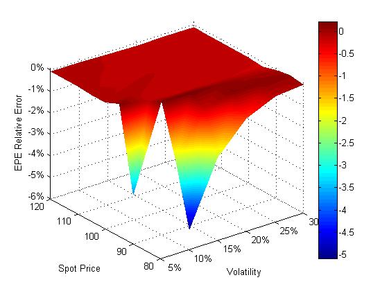
Figure 4: MC: EPE error $\varepsilon$ for European Call.

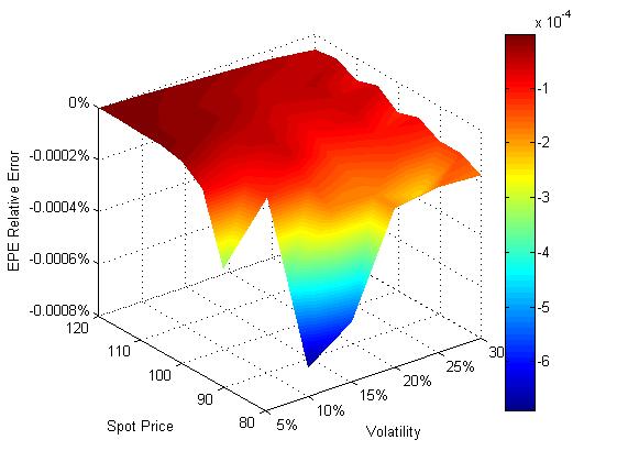
Figure 5: VQ: error $\varepsilon$ for European Call.

5.3 A portfolio of European options

In order to generalize techniques and results shown in the previous subsection, we are going to consider now a set of $n$ European options, i.e. a derivative portfolio, for which we will evaluate the Expected Exposure (EE) and the Expected Positive Exposure (EPE).

The portfolio may consist of call options and put options, related to a group of transactions with a single counterparty, which are subject to a legally enforceable bilateral netting arrangement. Such a set of derivatives is called netting set. From a mathematical point of view, such a choice means that the expected exposure is given by

$$EE=\left(\sum_{j=1}^{n}MtM(t)-V_{t}\right)^{+}\;,$$

unlike the case of no-netting portfolio setting, where the sum of the fair prices of European options represents the Mark-to-Market of the portfolio. The term $V_{t}$ represent the collateral value posted by the debtor, i.e. the counterparty with the negative Mark-to-Market portfolio at time t. In what follows we set $V_{t}=0$, therefore we deal with the netting agreement situation, supposing no collateral. Even if the set up can appear simple, this is not true, and the problem turns out to be rather challenging. That is because, generally speaking, one can not perform the analytical calculation of $EE_{k}$. In fact, also if the martingale property holds for each derivative in the portfolio, in the present case the positive part operator is effective, hence the future value is not simply the compounded current MtM.

For computational purposes, we consider $n=10$ European options, that is $5$ call options, the first, the third and the last one are of buy type, while the second and the fourth one are of sell type, and $5$ put options, namely, the first, the second and the last one of sell type and the remaining of buy type. To summarize, we have constructed a table with the features of the different options, see Table 10.

The software code is quite general to deal with any change in quantities, buy/sell, market and instrument parameters.

For the application we consider the following values:

• spot price $(S_{0}):$ $90,100,110$

• interest rate $(r):$ $3\%$

• volatility $(\sigma):$ $15\%,25\%,30\%$

• maturity $(T):$ one year

• time buckets: $\left\{0,\frac{1}{52},\frac{2}{52},\frac{3}{52},\frac{4}{52},\frac{2}{12},\frac{3}{12},\frac{6}{12},\frac{9}{12},1\right\}.$

	type	position	strike	maturity
Option 1	call	buy	$125$	1 year
Option 2	call	sell	$100$	1 year
Option 3	call	buy	$80$	1 year
Option 4	call	sell	$95$	1 year
Option 5	call	buy	$105$	1 year
Option 6	put	sell	$80$	1 year
Option 7	put	sell	$100$	1 year
Option 8	put	buy	$110$	1 year
Option 9	put	buy	$90$	1 year
Option 10	put	sell	$120$	1 year

Table 10: Description of the portfolio. The table summarizes the characteristics of the netting set

To better understand the characteristics of the portfolio, let us consider the following two figures, which show the portfolio profile for the different volatilities. It is a long style portfolio, with different levels of delta sensitivities.

Figure 6: MtM of the portfolio depending on volatility.

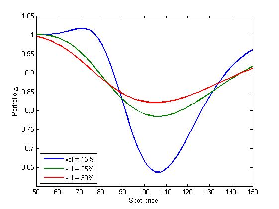
Figure 7: Delta of the portfolio depending on volatility.

The benchmark value for this application can not be a closed Black-Scholes approach. Hence we use a Monte Carlo-Sobol sequence with a large enough number of points as an acceptable pivot value. We use $10^{6}$ points. The vector quantization and the Monte Carlo techniques are tested with $10^{3}$ points.

As it was done in Subsection 5.2, in relation to the case of only one option, the comparison among the different procedures consists in analyzing the percent relative standard error (RSD) for the Monte Carlo approach and the percent relative error ($\varepsilon$) for the quantization technique.

	MC-Sobol $10^{6}$	Quantization		Monte Carlo		MC-Sobol $10^{3}$
t	EE	EE	$\varepsilon$	EE	RSD	EE	RSD
1w	0,0000	0,0000	NaN	0,0000	NaN	0,0000	NaN
2w	0,0000	0,0000	4,184%	0,0000	NaN	0,0002	99,950%
3w	0,0006	0,0006	-0,585%	0,0007	99,950%	0,0004	99,950%
1m	0,0030	0,0030	-0,021%	0,0022	70,933%	0,0060	58,952%
2m	0,0537	0,0537	0,033%	0,0425	22,046%	0,0586	20,217%
3m	0,1462	0,1463	0,048%	0,1254	15,505%	0,1552	15,306%
6m	0,5045	0,5045	0,010%	0,4539	10,512%	0,5054	10,581%
9m	0,8529	0,8529	-0,005%	0,8965	8,428%	0,8926	8,581%
1y	1,3863	1,3874	0,078%	1,2717	7,466%	1,4630	7,294%
EPE	0,7030	0,7033	0,040%	0,6698	-4,719%	0,7336	4,348%

Table 11: EPE: $S_{0}=90;\sigma=15\%.$

	MC-Sobol $10^{6}$	Quantization		Monte Carlo		MC-Sobol $10^{3}$
t	EE	EE	$\varepsilon$	EE	RSD	EE	RSD
1w	0,0001	0,0001	0,701%	0,0001	99,950%	0,0000	NaN
2w	0,0075	0,0075	0,032%	0,0074	54,701%	0,0093	64,637%
3w	0,0348	0,0348	-0,046%	0,0523	24,373%	0,0427	27,104%
1m	0,0817	0,0817	0,014%	0,0939	18,901%	0,0899	23,586%
2m	0,4319	0,4319	0,001%	0,4329	11,475%	0,4489	12,248%
3m	0,8119	0,8121	0,028%	0,7440	10,323%	0,8226	10,542%
6m	1,8836	1,8837	0,005%	1,7520	8,568%	1,9046	8,687%
9m	2,7611	2,7612	0,005%	2,9002	7,896%	2,8727	8,103%
1y	3,5191	3,5217	0,075%	3,4064	7,868%	3,5674	8,452%
EPE	2,1497	2,1505	0,034%	2,1185	-1,454%	2,1977	2,232%

Table 12: EPE: $S_{0}=90,\sigma=25\%.$

	MC-Sobol $10^{6}$	Quantization		Monte Carlo		MC-Sobol $10^{3}$
t	EE	EE	$\varepsilon$	EE	RSD	EE	RSD
1w	0,0013	0,0013	0,145%	0,0040	68,879%	0,0005	99,950%
2w	0,0291	0,0291	0,004%	0,0325	30,112%	0,0312	37,205%
3w	0,0981	0,0981	-0,013%	0,1321	18,842%	0,1157	19,728%
1m	0,1954	0,1954	-0,012%	0,2277	14,700%	0,2049	17,692%
2m	0,7796	0,7796	0,004%	0,7821	10,110%	0,7997	10,680%
3m	1,3415	1,3418	0,021%	1,2408	9,292%	1,3594	9,441%
6m	2,8256	2,8257	0,005%	2,6487	8,089%	2,8590	8,221%
9m	4,0074	4,0077	0,008%	4,2019	7,686%	4,1538	7,896%
1y	4,9419	4,9447	0,058%	4,8168	7,829%	5,0104	8,410%
EPE	3,1317	3,1325	0,027%	3,0981	-1,074%	3,1976	2,106%

Table 13: EPE: $S_{0}=90,\sigma=30\%.$

	MC-Sobol $10^{6}$	Quantization		Monte Carlo		MC sobol $10^{3}$
t	EE	EE	$\varepsilon$	EE	RSD	EE	RSD
1w	0,3565	0,3565	0,000%	0,3325	6,223%	0,3562	5,746%
2w	0,5758	0,5758	0,000%	0,5681	5,447%	0,5757	5,433%
3w	0,7463	0,7463	0,000%	0,7992	5,182%	0,7482	5,275%
1m	0,8904	0,8904	-0,003%	0,9439	5,022%	0,8889	5,266%
2m	1,3966	1,3966	0,000%	1,4407	4,793%	1,4016	5,007%
3m	1,7463	1,7463	0,004%	1,6845	4,950%	1,7351	5,051%
6m	2,5014	2,5014	0,003%	2,4279	4,960%	2,5149	5,097%
9m	3,0139	3,0138	-0,002%	3,0990	5,225%	3,0437	5,377%
1y	3,5845	3,5852	0,018%	3,5369	5,253%	3,6740	5,459%
EPE	2,5952	2,5954	0,007%	2,5865	-0,337%	2,6279	1,261%

Table 14: EPE: $S_{0}=100,\sigma=15\%.$

	MC-Sobol $10^{6}$	Quantization		Monte Carlo		MC-Sobol $10^{3}$
t	EE	EE	$\varepsilon$	EE	RSD	EE	RSD
1w	0,5510	0,5510	0,000%	0,5113	7,316%	0,5500	6,632%
2w	0,9683	0,9683	0,000%	0,9532	6,113%	0,9677	6,094%
3w	1,2999	1,2999	0,000%	1,4062	5,717%	1,2986	5,884%
1m	1,5831	1,5831	0,001%	1,6824	5,537%	1,5901	5,777%
2m	2,5909	2,5909	0,001%	2,6600	5,273%	2,5990	5,501%
3m	3,2975	3,2977	0,004%	3,1569	5,466%	3,2792	5,561%
6m	4,8611	4,8614	0,006%	4,6669	5,563%	4,8787	5,676%
9m	5,9723	5,9725	0,002%	6,1526	5,816%	6,0292	6,002%
1y	6,8363	6,8377	0,020%	6,6731	6,139%	6,9781	6,320%
EPE	5,0094	5,0099	0,009%	4,9625	-0,936%	5,0627	1,065%

Table 15: EPE: $S_{0}=100,\sigma=25\%.$

	MC-Sobol $10^{6}$	Quantization		Monte Carlo		MC-Sobol $10^{3}$
t	EE	EE	$\varepsilon$	EE	RSD	EE	RSD
1w	0,7348	0,7348	0,000%	0,6826	7,124%	0,7335	6,474%
2w	1,2651	1,2651	0,000%	1,2462	6,034%	1,2643	6,021%
3w	1,6844	1,6844	-0,001%	1,8210	5,684%	1,6836	5,844%
1m	2,0418	2,0418	0,001%	2,1698	5,522%	2,0507	5,765%
2m	3,3126	3,3126	0,001%	3,3997	5,308%	3,3231	5,541%
3m	4,2047	4,2049	0,004%	4,0221	5,531%	4,1822	5,630%
6m	6,1892	6,1895	0,005%	5,9304	5,685%	6,2124	5,795%
9m	7,6209	7,6210	0,002%	7,8537	5,953%	7,7022	6,134%
1y	8,6815	8,6828	0,015%	8,4780	6,330%	8,8203	6,549%
EPE	6,3807	6,3811	0,007%	6,3196	-0,957%	6,4407	0,941%

Table 16: EPE: $S_{0}=100,\sigma=30\%.$

	MC-Sobol $10^{6}$	Quantization		Monte Carlo		MC-Sobol $10^{3}$
t	EE	EE	$\varepsilon$	EE	RSD	EE	RSD
1w	5,9931	5,9931	0,000%	5,9450	0,786%	5,9939	0,777%
2w	5,9972	5,9972	0,000%	6,0020	1,095%	5,9974	1,105%
3w	6,0053	6,0053	0,000%	6,0699	1,372%	6,0046	1,350%
1m	6,0194	6,0194	0,000%	6,1167	1,537%	6,0213	1,546%
2m	6,1483	6,1482	-0,001%	6,3028	2,048%	6,1578	2,136%
3m	6,3084	6,3083	-0,001%	6,2873	2,407%	6,3192	2,483%
6m	6,7919	6,7918	-0,002%	6,7474	3,050%	6,7916	3,188%
9m	7,1835	7,1835	0,000%	7,2932	3,677%	7,2228	3,721%
1y	7,5898	7,5915	0,022%	7,4585	4,085%	7,5753	4,210%
EPE	6,9306	6,9310	0,005%	6,9284	-0,031%	6,9385	0,114%

Table 17: EPE: $S_{0}=110,\sigma=15\%.$

	MC-Sobol $10^{6}$	Quantization		Monte Carlo		MC-Sobol $10^{3}$
t	EE	EE	$\varepsilon$	EE	RSD	EE	RSD
1w	6,5122	6,5122	0,000%	6,4141	1,465%	6,5134	1,439%
2w	6,5989	6,5989	0,000%	6,6139	1,926%	6,6015	1,950%
3w	6,7315	6,7315	0,000%	6,8607	2,310%	6,7373	2,273%
1m	6,8813	6,8813	0,000%	7,0735	2,479%	6,8863	2,514%
2m	7,5927	7,5927	0,000%	7,8513	2,975%	7,5995	3,131%
3m	8,1894	8,1895	0,001%	8,1085	3,360%	8,2180	3,442%
6m	9,6447	9,6446	-0,001%	9,4633	3,984%	9,6789	4,093%
9m	10,7365	10,7363	-0,002%	10,9562	4,531%	10,7812	4,626%
1y	11,5732	11,5745	0,012%	11,4042	4,941%	11,5706	5,132%
EPE	9,8664	9,8666	0,003%	9,8547	-0,118%	9,8887	0,226%

Table 18: EPE: $S_{0}=110,\sigma=25\%.$

	MC-Sobol $10^{6}$	Quantization		Monte Carlo		MC-Sobol $10^{3}$
t	EE	EE	$\varepsilon$	EE	RSD	EE	RSD
1w	6,7056	6,7056	0,000%	6,5844	1,762%	6,7063	1,727%
2w	6,8948	6,8948	0,000%	6,9154	2,237%	6,8984	2,270%
3w	7,1282	7,1282	0,000%	7,3020	2,627%	7,1311	2,602%
1m	7,3679	7,3680	0,000%	7,6149	2,783%	7,3787	2,836%
2m	8,3987	8,3987	0,000%	8,6959	3,263%	8,4147	3,434%
3m	9,2137	9,2140	0,003%	9,0911	3,657%	9,2276	3,754%
6m	11,1493	11,1492	-0,001%	10,8929	4,279%	11,1882	4,389%
9m	12,5989	12,5984	-0,003%	12,8948	4,798%	12,6484	4,921%
1y	13,6675	13,6689	0,010%	13,4530	5,231%	13,7136	5,432%
EPE	11,4158	11,4160	0,002%	11,3947	-0,185%	11,4523	0,320%

Table 19: EPE: $S_{0}=110,\sigma=30\%.$

Below we present a couple of figures which clearly show how the VQ technique performs with an excellent accuracy over the different situations. It is worth to observe that, for some very deep out of the money situation, the Monte Carlo simulations shows a huge relative standard error. This occurs when the value of EE is next to zero. We remember that when the EE is very small, no effective counterparty risk has to be faced by the bank, hence, the magnitude of the error is not as dramatic as it seems from a numerical perspective.

Eventually, we plotted the percent relative error $\varepsilon$ and the percent relative standard error RSD, in order to compare, once again, the quantization technique and the Monte Carlo method, showing the excellent accuracy of the former approach, when compared with the latter.

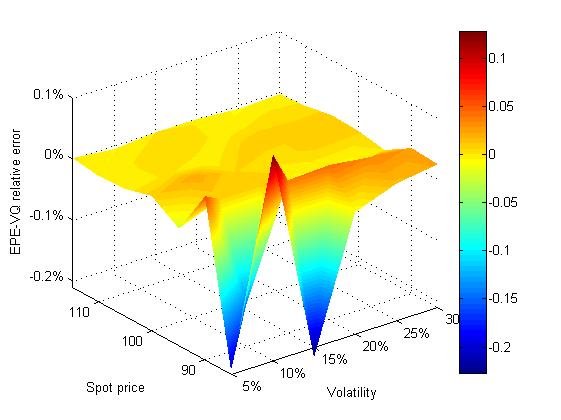
Figure 8: VQ: EPE error $\varepsilon$ for portfolio

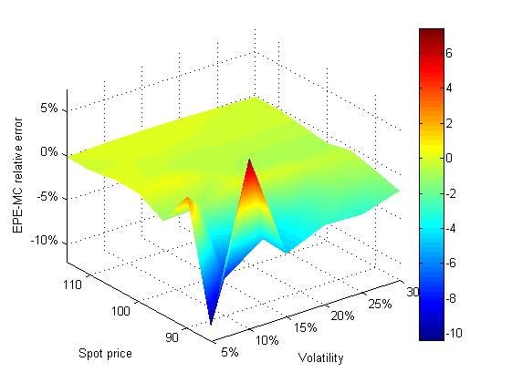
Figure 9: MC: EPE relative error $RSD$ for portfolio

6 Conclusions and Further Research

In the present work we show how the quantization approach outperforms the classical Monte Carlo methods in the CCR field. The counterparty risk field poses a lot of theoretical and practical challenges. A whole portfolio of derivatives must be evaluated in the future, for several time steps and many scenarios, in order to get some useful risk figures. This large amount of computations can be solved by improving the technologies or the algorithmic strategies.

At the best of our knowledge, this is the first work which exploits the quantization approach in this area. The quantization has been intensively tested in the last decade in some pricing problems for different complex situations: American style options, multidimensional assets, credit derivatives. Despite this first study covers some simple derivatives and small dimension portfolios, the quantization seems to be very promising. Given an equivalent computational effort, it is undoubtedly better than the standard Monte Carlo simulation and some of its refinements such as the Sobol sequences.

Nevertheless, further research is needed. As the next step, we aiming at treating more involved portfolios and payoffs, as in the case of path dependent options, where the quantization tree could be a competitor of binomial and trinomial trees. Moreover, concerning portfolios depending on many underlyings, there are issues related to the choice of a coherent set of quantized paths that has to be fixed.

Finally, numerical extensions as to be taken into account in order to pass from the accuracy comparison, given the same computational effort, to the search of the quantization tradeoff, namely an estimate of its relative effort saving, given the same accuracy.

References

- [1] BCBS (2006) “International Convergence of Capital Measurement and Capital Standards”, Basel Committee Paper 128.
- [2] BCBS (2011) “Basel III: A global regulatory framework for more resilient banks and banking systems”, Basel Committee Paper, 189
- [3] BCBS (2014) “The standardized approach for measuring counterparty credit risk exposures”, Basel Committee Paper 279
- [4] Bally V., Pagès G., Printemps J. (2010) “A quantization tree method for pricing and hedging multi-dimensional American options”, Working Paper
- [5] Black F., Scholes M. (1973) “The Pricing of Options and Corporate Liabilities”, Journal of Political Economy 81(3), 637–654.
- [6] Bucklew J.A., Wise G.L. (1982) “Multidimensional asymptotic quantization theory with power distortion”, IEEE Trans. Inform. Theory, 28(2), 239–247.
- [7] Caflisch R.E., Morokoff, W.J. (1995) “Quasi-Monte Carlo integration”, J. Comput. Phys. 122(2), 218–230.
- [8] Castagna A. (2012) “Fast computing in the CCR and CVA measurement”, IASON ALGO, Working Paper.
- [9] Cesari G. (2009) Modeling, Pricing and Hedging Counterparty Credit Exposure, Springer Finance Editor.
- [10] Dupire B. (1994), “Pricing with a smile”, Risk, January, 18–20.
- [11] Gersho A., Gray R. (1982) “IEEE on Information Theory, Special Issue on Quantization”, 28.
- [12] Hagan P. et al (2002), “Managing Smile Risk”, Wilmott Magazine.
- [13] Heston S. (1993), “A Closed-Form Solution for Options with Stochastic Volatility with Applications to Bond and Currency Options”, The Review of Financial Studies 6(2), 327–343.
- [14] IFRS (2013), “IFRS 13 Fair Value Measurement”, IFRS Technical Paper
- [15] A.Mikes, (2013), “The Appeal of the Appropriate: Accounting, Risk Management, and the Competition for the Supply of Control Systems”, Harward Business School - working papers, 115(12).
- [16] Pagès G., Printemps J., Pham H. (2004), “Optimal quantization methods and applications to numerical problems in finance”, Handbook on Numerical Methods in Finance, Birkh auser, 253–298.
- [17] Pagès G., Luschgy H. (2006), “Functional quantization of a class of Brownian diffusions: A constructive approach”, Stochastic processes and their Applications, Elsevier, 116, 310–336.
- [18] Pagès G., Wilbertz B. (2012), “Intrinsic stationarity for vector quantization: Foundation of dual quantization”, SIAM Journal on Numerical Analysis, 747–780.
- [19] Pagès G., Wilbertz B. (2011), “GPGPUs in computational finance: Massive parallel computing for American style options”, Working paper.
- [20] Pykhtin M., Zhu S. (2007), “A Guide to Modelling Counterparty Credit Risk”, GARP publication.
- [21] Sellami, A. (2005) “Mèthodes de quantification optimale pour le filtrage et applications á la finance”, Applied mathematics: Universitè Paris Dauphine.
- [22] Shreve, S., (2004) Stochastic Calculus for Finance II. Continuous time models, Springer Finance series
- [23] Zador, P.L. (1963), Development and evaluation of procedures for quantizing multivariate distributions, Ph.D. dissertation, Stanford Univ. (USA).
- [24] Zador, P.L. (1982), “Asymptotic quantization error of continuous signals and the quantization dimension”, IEEE Trans. Inform. Theory, 28(2).