The VIMOS Ultra Deep Survey: Ly$\alpha$ Emission and Stellar Populations of Star-Forming Galaxies at 2 $<$ $z$ $<$ 2.5 

The aim of this paper is to investigate spectral and photometric properties of 854 faint ($i_{AB}$ $\lesssim$ 25 mag) star-forming galaxies (SFGs) at 2 $<$ $z$ $<$ 2.5 using the VIMOS Ultra-Deep Survey (VUDS) spectroscopic data and deep multi-wavelength photometric data in three extensively studied extragalactic fields (ECDFS, VVDS, COSMOS). These SFGs were targeted for spectroscopy based on their photometric redshifts. The VUDS spectra are used to measure the UV spectral slopes ($\beta$) as well as Ly$\alpha$ equivalent widths (EW). On average, the spectroscopically measured $\beta$ (–1.36$\pm$0.02), is comparable to the photometrically measured $\beta$ (–1.32$\pm$0.02), and has smaller measurement uncertainties. The positive correlation of $\beta$ with the Spectral Energy Distribution (SED)-based measurement of dust extinction E_s(B–V) emphasizes the importance of $\beta$ as an alternative dust indicator at high redshifts. To make a proper comparison, we divide these SFGs into three subgroups based on their rest-frame Ly$\alpha$ EW: SFGs with no Ly$\alpha$ emission (SFG_N; EW $\leq$ 0Å), SFGs with Ly$\alpha$ emission (SFG_L; EW $>$ 0Å), and Ly$\alpha$ emitters (LAEs; EW $\geq$ 20Å). The fraction of LAEs at these redshifts is $\sim$10%, which is consistent with previous observations. We compared best-fit SED-estimated stellar parameters of the SFG_N, SFG_L and LAE samples. For the luminosities probed here ($\sim$L^∗), we find that galaxies with and without Ly$\alpha$ in emission have small but significant differences in their SED-based properties. We find that LAEs have less dust, and lower star-formation rates (SFR) compared to non-LAEs. We also find that LAEs are less massive compared to non-LAEs, though the difference is smaller and less significant compared to the SFR and E_s(B–V). When we divide the LAEs based on their Spitzer/IRAC 3.6$\mu$m fluxes, we find that the fraction of IRAC-detected (m_3.6 $\lesssim$ 25 mag) LAEs is much higher than the fraction of IRAC-detected narrow band (NB)-selected LAEs at $z$ $\simeq$ 2–3. This could imply that UV-selected LAEs host a more evolved stellar population, which represents a later stage of galaxy evolution compared to NB-selected LAEs.

1 Introduction

In the last decade, large numbers of star-forming galaxies (SFGs) — selected using the Lyman break color technique and/or the photometric redshift technique — were identified and studied at $z$ $\gtrsim$ 3 using deep photometric surveys (e.g., Bouwens et al., 2007; Hathi et al., 2008a; Ouchi et al., 2009; McLure et al., 2010; Yan et al., 2010; Finkelstein et al., 2010; Hathi et al., 2012; Tilvi et al., 2013; Ellis et al., 2013; Finkelstein et al., 2013). This large reservoir of SFGs spanning a very large redshift range ($z$ $\simeq$ 3–8), and brightnesses (24–29 mag), has tremendous impact on our understanding of the process of galaxy formation and evolution (e.g., Maioline et al., 2008; Ilbert et al., 2013; Speagle et al., 2014; Finkelstein et al., 2015). However, the spectroscopic and photometric studies for most of these galaxies are very challenging because of their faint magnitudes and lack of high resolution multi-wavelength data. Therefore, detailed studies of SFGs at lower redshifts ($z$ $<$ 3) using ground-based spectroscopy and multi-wavelength photometry are vital for understanding physical processes at the peak epoch of star formation as well as to better understand high redshift galaxy formation.

The study of SFGs at $z$ $\sim$ 2 has a significant impact on our understanding of galaxy properties. First, these SFGs are at redshifts corresponding to the peak epoch ($z$ $\sim$ 1–3) of the global star formation rate (SFR) density (e.g., Madau et al., 1998; Cucciati et al., 2012; Madau & Dickinson, 2014), where $>$50% of the stars in the present-day Universe formed, and is a perfect epoch to study star formation processes. Second, this cosmologically interesting redshift is also where we have access to a wealth of multi-wavelength data, and rest-frame optical spectroscopy, to study galaxy properties that we cannot investigate at higher redshifts with current technology. The major advantage of identifying and studying various physical properties — including star formation properties — of these SFGs is that they can be investigated in rest-frame UV as well as rest-frame optical filters. Third, these galaxies are likely lower redshift analogs of the high redshift SFGs, and putting in a context such analysis will help to shed light on the process of reionization in the early Universe (e.g., Labbé et al., 2010; Stark et al., 2010) and how the first galaxies formed. Finally, the redshift $z$ $\sim$ 2 is the lowest redshift where we can identify and study Ly$\alpha$ in emission from ground-based spectroscopy and these galaxies are bright enough for extensive spectroscopic studies on 8-10m class telescopes.

Spectroscopy is an essential and powerful tool to fully understand galaxy properties but the underlying photometric selection of galaxies can bias the spectroscopic sample properties. The primary techniques to select SFGs by color at $z$ $\simeq$ 2 are: (1) sBzK (using the $B$, $z$, $K$ bands, Daddi et al., 2004, 2007), (2) BX/BM (using the $U$, $G$, $R$ bands, Steidel et al., 2004; Adelberger et al., 2004), and (3) LBG (using the bands which bracket the redshifted Lyman limit, Hathi et al., 2010; Oesch et al., 2010). The other main approach is based on the magnitude/flux limit and/or photometric redshift selection, as used by many spectroscopic surveys such as, VVDS, GMASS, zCOSMOS (e.g., Le Fèvre et al., 2005; Lilly et al., 2007; Kurk et al., 2009; Le Fèvre et al., 2013). On the other hand, SFGs are also selected based on the emission-line/Narrow-band (NB) techniques (e.g., Guaita et al., 2010; Berry et al., 2012; Vargas et al., 2014) which bracket strong emission lines at $z$ $\simeq$ 2. All these approaches select star-forming galaxies, and yield insight into the star-forming properties of these galaxies, but they have differing selection biases, and therefore, these samples do not completely overlap (see Ly et al., 2011; Haberzettl et al., 2012, for details). Therefore, it is essential to apply a well defined selection leading to the identification of a population with a broad range of galaxy properties, which can then be compared to similar galaxies at higher redshifts.

The comparison of stellar populations of (strong) Ly$\alpha$ emitting galaxies (LAEs), primarily selected based on the NB imaging technique, and non-LAEs (with weak or no Ly$\alpha$-emission), primarily selected based on photometric colors that mimic a break (i.e., Lyman break galaxies, LBGs), has yielded diverse and inconclusive results. Gawiser et al. (2006) found that NB-selected LAEs at $z$ $\simeq$ 3.1 are less massive and less dusty compared to continuum selected LBGs suggesting that LAEs represent an early stage of an evolutionary sequence where galaxies gradually become more massive and dusty due to mergers and star formation (Gawiser et al., 2007). This conclusion is consistent with high specific star formation rates (SSFR, SFR per unit mass) of NB-selected LAEs found by Lai et al. (2008) relative to LBGs at the same redshift. On the other hand, Finkelstein et al. (2009) found a range of dust extinctions in a sample of 14 NB-selected LAEs at $z$ $\simeq$ 4.5, which is not consistent with LAEs being the first galaxies in the evolutionary sequence. Similarly, Nilsson et al. (2011) used 171 NB-selected LAEs at $z$ $\simeq$ 2.25 and concluded that the stellar properties of LAEs are different from those at higher redshift and that they are diverse. They also believe that Ly$\alpha$ selection could be tracing different galaxies at different redshifts, which is consistent with the findings of Acquaviva et al. (2012). Lai et al. (2008) found that IRAC-detected LAEs are significantly older (age $\gtrsim$ 1 Gyr) and more massive (mass $\sim$ 10¹⁰ M_⊙) compared to IRAC-undetected LAEs at $z$ $\simeq$ 3.1, which lead them to suggest that the IRAC-detected LAEs may be a lower-mass extension of the LBG population. These studies show heterogeneity of NB-selected LAEs, and comparison between these objects and continuum selected LBGs continues to be the subject of many new studies.

Various authors have compared stellar population properties of LAEs and non-LAEs in UV flux-limited samples (e.g., Shapley et al., 2001; Erb et al., 2006; Pentericci et al., 2007; Reddy et al., 2008; Kornei et al., 2010). Shapley et al. (2001) generated rest-frame UV composite spectra of LBGs at $z$ $\simeq$ 3 dividing subsamples in ‘young’ ($t\leq$ 35 Myr) and ‘old’ ($t\geq$ 1 Gyr) galaxies. They found that younger galaxies have weaker Ly$\alpha$ emission, are more dusty, and less massive compared to older galaxies. On the other hand, the analysis of Erb et al. (2006) of the composite UV spectra for $\sim$60 SFGs at $z$ $\simeq$ 2 concluded that, on average, objects with lower stellar mass had stronger Ly$\alpha$ emission line than more massive objects. Using a sample of 14 UV-selected galaxies at $z$ $\simeq$ 2–3 with Ly$\alpha$ equivalent width (EW) $\geq$ 20Å, Reddy et al. (2008) found no significant difference in the stellar populations of strong Ly$\alpha$-emitters compared to the rest of the sample. At higher redshifts, Pentericci et al. (2007) found that, in general, younger galaxies at $z$ $\simeq$ 4 showed Ly$\alpha$ in emission while older galaxies showed Ly$\alpha$ in absorption. More recently, Kornei et al. (2010) used 321 LBGs at $z$ $\simeq$ 3 to study the relationship between Ly$\alpha$-emission and stellar populations. Based on their analysis, they concluded that objects with strong Ly$\alpha$-emission are older, lower in SFR, and less dusty compared to objects with weak or no (Ly$\alpha$ in absorption) Ly$\alpha$-emission. The results of these studies emphasize that the exact relation between stellar populations and Ly$\alpha$-emission is still not yet fully understood.

In this paper we use spectroscopic data from the VIMOS Ultra-Deep Survey (VUDS), to study the spectral & photometric properties of a large sample of faint SFGs at 2 $<$ $z$ $<$ 2.5 ($z_{median}$ $\simeq$ 2.3). VUDS recently obtained data for $\sim$10000 galaxies over an area of $\sim$1 deg² using the 8.2m Very Large Telescope (VLT). The VUDS observations were performed in the well-studied COSMOS (Scoville et al., 2007; Koekemoer et al., 2007) and ECDFS (Giavalisco et al., 2004; Rix et al., 2004) fields now partly covered with HST/WFC3 by CANDELS (Grogin et al., 2011; Koekemoer et al., 2011), and in the VVDS-02h field (Le Fèvre et al., 2004; McCracken et al., 2003). These fields have extensive multi-wavelength data. We extract a sample of 854 galaxies with confirmed spectroscopic redshifts at 2 $<$ $z$ $<$ 2.5, uniformly selected from their continuum properties with $i_{AB}$ $\lesssim$ 25 mag. The goal of this paper is to study the physical properties of these SFGs which include galaxies with and without Ly$\alpha$ emission.

This paper is organized as follows: In §2, we summarize the VUDS observations, and discuss 2 $<$ $z$ $<$ 2.5 sample selection as well as its basic properties. In §3, we fit observed rest-frame UV VUDS spectra at 2 $<$ $z$ $<$ 2.5 to measure the UV spectral slope, and discuss its correlation with the E_s(B–V), stellar mass, and UV absolute magnitude. In §4, we discuss differences in stellar population properties between galaxies with and without Ly$\alpha$ in emission. In §5, we investigate correlations between derived physical parameters (UV absolute magnitude, SFRs, E_s(B–V), stellar mass, and UV spectral slope) as a function of rest-frame Ly$\alpha$ EW for SFGs and their implications on our understanding of these galaxies. Results are discussed in §6, and we conclude with a summary in §7.

Throughout this paper, we assume the standard cosmology with $\Omega_{m}$=0.3, $\Omega_{\Lambda}$=0.7 and $H_{\rm 0}$=70 km s^-1 Mpc^-1. This corresponds to a look-back time of $\sim$10.4 Gyr at $z$ $\simeq$ 2. Magnitudes are given in the AB system (Oke & Gunn, 1983).

2 Data and Sample Selection

The VUDS observations (Le Fèvre et al., 2015) were done using the low-resolution multi-slit mode of VIMOS on the VLT. A total of 15 VIMOS pointings ($\sim$224 arcmin² each, $\sim$1 deg² total) were observed with both the LRBLUE and LRRED grisms covering the full wavelength range from 3650Å to 9350Å in three fields (ECDFS, VVDS-02h, COSMOS). The total exposure time per pointing was 14h in each grism. This paper is based on $\sim$80% of the data, which is the amount processed at the time of writing this paper. Details of these observations and the reduction process are described in Le Fèvre et al. (2015).

2.1 Photometry

VUDS targeted three well-studied extragalactic fields with extensive multi-wavelength photometry. Details are given in Le Fèvre et al. (2015). Here, we briefly summarize the most relevant imaging observations for these three fields.

The COSMOS field was observed with HST/ACS in the F814W filter (Scoville et al., 2007; Koekemoer et al., 2007). Deep ground based imaging includes observations in $u^{*},B,V,g^{+},r^{+},i^{+},z^{+}$ bands from Subaru and CFHT. Details about these and other publicly available multi-wavelength observations are available at COSMOS websites. The UltraVista survey is acquiring very deep near-infrared imaging in the $YJHK$ bands using the VIRCAM camera on the VISTA telescope (McCracken et al., 2012), while deep Spitzer/IRAC observations are available through the SCOSMOS (Sanders et al., 2007) program. The CANDELS survey (Grogin et al., 2011; Koekemoer et al., 2011) also provided WFC3 NIR photometry in the smaller, central part of the COSMOS field.

The ECDFS field has been the target of many multi-wavelength surveys in the last decade. The central part of the field, covering $\sim$ 160 arcmin², has HST/ACS observations (Giavalisco et al., 2004) combined with the recent CANDELS HST/WFC3 observations in the near-infrared bands (Koekemoer et al., 2011). The ECDFS field is covered by deep $UBVRIzJHK$ imaging as part of MUSYC and other surveys in this field (Cardamone et al., 2010, and references therein). The SERVS program obtained medium-deep observations in 3.6$\mu$m and 4.5$\mu$m (Mauduit et al., 2012), which complement those obtained by the GOODS team (PI: M. Dickinson) at 3.6, 4.5, 5.6, and 8.0$\mu$m.

The VVDS-02h field has deep optical imaging from CFHT in the $u^{*},g^{\prime},r^{\prime},i^{\prime},z^{\prime}$ bands (e.g., Cuillandre et al., 2012) as part of the CFHT Legacy Survey. Deep near-infrared imaging in the $JHK_{s}$ bands has been obtained with WIRCam on CFHT as part of the WIRCam Deep Survey (WIRDS; Bielby et al., 2012). The deep near-infrared imaging data (3.6$\mu$m and 4.5$\mu$m) has been obtained with Spitzer/IRAC as part of the SERVS program (e.g., Mauduit et al., 2012). We refer the reader to Lemaux et al. (2014a) for a detailed description of multi-wavelength imaging data in VVDS-02h field.

2.2 VUDS Target Selection

The primary selection criterion for galaxies in the VUDS program was photometric redshifts ($z_{phot}$ + 1$\sigma$ $\geq$ 2.4), which are accurate to within 5% errors for these well-studied fields (e.g., Ilbert et al., 2009; Coupon et al., 2009; Dahlen et al., 2010). For high redshift ($z$ $\gtrsim$ 2.5) targets, this photometric redshift selection was supplemented by color criteria (e.g., LBG/$ugr$, LBG/$gri$, LBG/$riz$), if the objects satisfied these color criteria but were not selected from the primary photometric redshift criterion. The fraction of targets selected for each criterion at different redshifts is shown in Table 2 of Le Fèvre et al. (2015). At 2 $<$ $z$ $<$ 2.5, all spectroscopic targets were selected solely based on the photometric redshift criterion. Therefore, the targets for the VUDS program include a representative sample of all star-forming galaxies at a particular redshift within a given magnitude limit ($i_{AB}$ $\lesssim$ 25 mag, with some galaxies as faint as $i_{AB}$ $\sim$ 27 mag). It is important to note that the target selection is not based on any particular emission line of a galaxy but on continuum magnitude. A detailed discussion about the target selection, reliability of the redshift measurements and corresponding quality flags is presented in Le Fèvre et al. (2015).

2.3 Sample Selection

For this paper, the primary selection criterion for the sample of SFGs from the VUDS spectroscopic data is the redshift. All objects between $z$ = 2 and $z$ = 2.5 are selected in the final sample, keeping only the best reliability flags (2,3,4,9) — which gives very high probability (75-85%, 95-100%, 100%, 80%, respectively; see Le Fèvre et al. 2015 for details) for these redshifts to be correct. The total number of galaxies selected at 2 $<$ $z$ $<$ 2.5 for the current work is 854. Based on a simple nearest-neighbor matching to the most recent catalogs in each field (e.g., Chiappetti et al., 2005; Elvis et al., 2009; Xue et al., 2011), we find that our sample contains minimal contamination from X-ray AGN ($\lesssim$1%), which suggests that our sample is comprised almost exclusively of galaxies without powerful X-ray AGN activity. We also checked for obscured AGN using Donley et al. (2012) Spitzer/IRAC criteria, and found that $\sim$3% of galaxies in our sample could host AGN based on this criteria. Some of these IRAC-selected AGN are also X-ray AGN, so after removing these overlapping AGN we end up with $\sim$2% of additional AGN candidates using the Donley et al. IRAC criteria. This confirms that our SFGs sample has minimum contamination ($\lesssim$3%) from AGN identified based on their X-ray emission and IRAC colors. This does not rule out the presence of other types of AGN or AGN-like activity in our sample (e.g., Cimatti et al., 2013; Lemaux et al., 2010), but such phenomena do not, typically, dominate the UV/optical/NIR light of their host galaxies, which is the important point for our analysis.

The Le PHARE software package (Arnouts et al., 1999; Ilbert et al., 2006) was used to fit the broad-band observed Spectral Energy Distributions (SEDs) with synthetic stellar population models. We use BC03 (Bruzual & Charlot, 2003) templates to generate a set of stellar population models assuming a Chabrier initial mass function (IMF; Chabrier, 2003), and fixed the spectroscopic redshift, while varying metallicity ($Z$ = 0.4 and 1 $Z_{\odot}$), age (0.05 Gyr $\leq$ $t$ $\leq$ $t_{H}$), dust extinction (0 $\leq$ E_s(B–V) $\leq$ 0.7 mag) — using a Calzetti et al. (2000) attenuation law or, in some cases, Calzetti law + 2175Å bump — and $e$-folding timescale ($\tau$ = 0.1–30 Gyr, i.e., from instantaneous burst to continuous star formation) for a star-formation history (SFH) $\propto$ exp(-t/$\tau$). We also included two delayed SFH models with peaks at 1 and 3 Gyr. The Le PHARE code assumes the Madau (1995) prescription to estimate inter-galactic medium (IGM) opacity. From the best-fit model, we estimate stellar mass, dust extinction E_s(B–V), SFRs, and SSFR for each galaxy. The UV absolute magnitudes are measured using the prescription of Ilbert et al. (2005) and are not corrected for the internal dust extinction.

We emphasize that SFRs and E_s(B–V)/dust inferred from fitting BC03 models to the SED of galaxies give only a rough estimate of these physical parameters. To understand the effect of medium-band filters as well as other input quantities on the best-fit SED parameters, we compared our SFR and E_s(B–V) measurements with two different surveys that use medium band photometry: (1) NEWFIRM Medium Band Survey (NMBS) in the COSMOS field (Whitaker et al., 2012a) and (2) COSMOS SED measurements using 30 photometric bands (Ilbert et al., 2009), which includes broad-band as well as intermediate and narrow bands in the optical and NIR. For NMBS data, we have a small number ($\sim$20) of galaxies matching both catalogs. For these galaxies, we find that, on average, SFRs differ by $\sim$0.5 dex (factor of $\sim$3), and A_v (E_s(B–V)) differ by $\lesssim$ 0.2 ($\lesssim$ 0.07). For COSMOS 30-band data which has larger sample ($\sim$300) of galaxies, we find that, on average, SFRs differ by $\sim$0.2 dex (factor of $\sim$2), and A_v (E_s(B–V)) differ by $\lesssim$ 0.15 ($\lesssim$ 0.05). It is crucial to note that NMBS uses slightly different input set-up for SED-fitting e.g., slightly different SFHs, different choice of extinction laws, different metallicity range, use of photometric redshifts, compared to what we use, so these choices of input parameters will also affect SFRs and dust measurements. Therefore, the larger difference between NMBS and our SED measurements is not only due to photometric bands. As for COSMOS 30-band, we kept all the input parameters same as in the broad-band photometry SED fitting but changed only the input photometric bands, so other effects do not play any role, and we see much smaller differences. These comparisons show that the uncertainties in SFRs and dust measurements due to the choice of photometric bands and other input SED parameters could be as high as factor of $\sim$3 for SFRs and $\sim$0.2 mag for A_v (or $\sim$0.07 for E_s(B–V)), which is typically expected for the SED-fitting process (e.g., Muzzin et al., 2010; Mostek et al., 2012). It is important to mention that these uncertainties are inherent in the SED fitting process and are not unique to this study. Moreover, this study is based on the relative measurements of three different galaxy populations and as long as there are no drastic differences in the IMF or SFHs of these populations, these systematic uncertainties does not play a significant role in the conclusions of this paper.

The contribution of major emission lines in different filters has been included in the models of the Le PHARE code. We use these templates with emission lines to carry out SED fitting. Neglecting emission lines during the SED fitting process can overestimate the best-fit stellar ages and stellar masses by up to $\sim$ 0.3 dex (e.g., Schaerer & de Barros, 2009; Finkelstein et al., 2011; Atek et al., 2011). The Le PHARE code accounts for the contribution of emission lines with a simple recipe based on the Kennicutt (1998) relations between the SFR and UV luminosity, H$\alpha$ and [OII] lines. The code includes the Ly$\alpha$, H$\alpha$, H$\beta$, [OII], OIII[4959] and OIII[5007] lines with different line ratios with respect to the [OII] line, as described in Ilbert et al. (2009).

2.4 Sample Properties

Figure 1 shows distributions of spectroscopic redshifts and far-UV (1500Å) absolute magnitudes (M₁₅₀₀) for the full SFG sample at 2 $<$ $z$ $<$ 2.5. The median M₁₅₀₀ of the sample is –20.22 mag, while the median redshift is 2.320. The figure also shows the evolving characteristic magnitude M^∗ as a function of the redshift, as derived from the compilation of Hathi et al. (2010). The M${}^{*}\pm$1 mag range covers most of our data which implies that we are probing luminosities around L^∗ at these redshifts. The shape of the redshift distribution is dictated, in part, by the selection function used to select target galaxies for VUDS. The main selection criteria under which primary targets are selected, is $z_{phot}$ + 1$\sigma$ $\geq$ 2.4. Therefore, at lower redshifts (2 $<$ $z$ $<$ 2.4) we are on the tail of the probability distribution of photometric redshifts, and this explains the decreasing number of galaxies at $z$ $<$ 2.4. This bias equally affects all galaxies — galaxies with and without Ly$\alpha$ in emission — so the general results in this paper, making relative comparisons of the two populations, are not affected by this selection bias. The second reason for the small number of galaxies close to the lower limit of our redshift range could be the sensitivity of the VIMOS instrument which starts to decrease dramatically below 3800Å. This means that we might not be able to properly identify continuum breaks, important features to secure the redshift, below redshift $z$ $\lesssim$ 2.15. In this redshift range, we might be biased in favor of strong Ly$\alpha$ emitters as we could still identify those even at $z$ $\lesssim$ 2.15. To check this sample selection effect, we cut our sample at redshift $z$ = 2.15. By doing so, we remove $\sim$10% of galaxies from the full sample, which is very small compared to the large sample size of VUDS galaxies. This small change in number of galaxies does not change our final results. Therefore, the results presented in this paper are not affected by this selection bias.

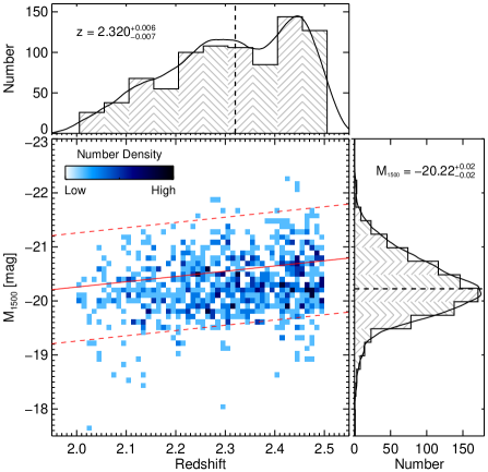
Figure 1: Redshift versus UV absolute magnitude (M₁₅₀₀) for spectroscopically confirmed SFGs at 2 $<$ $z$ $<$ 2.5 from VUDS. The median M₁₅₀₀ of the sample is –20.22 mag, the median redshift is 2.320. The quoted uncertainties are the errors on the median ($1.253\,\times\,\sigma/\sqrt{\rm N_{\rm gal}}$) estimated from the 1$\sigma$ dispersion of the distribution and the total number of galaxies, where $\pm$ 1$\sigma$ corresponds to the range between the 16th and the 84th percentile values of the distribution. The red solid line indicates the evolving M^∗ (characteristic magnitude) as a function of redshift as derived from the compilation of Hathi et al. (2010). The dashed red lines indicate M${}^{*}\pm$1 mag. The black solid curve on the histogram is the kernel density estimation (KDE) of the distribution, which is a smoother non-parametric density estimator compared to the histogram and is not affected by the bin-size or the end points of the bins. The density of points is color-coded as shown in the color-bar.

Figure 2 shows distributions of stellar mass and SFR for the full SFG sample at 2 $<$ $z$ $<$ 2.5. The median stellar mass of the sample is $\sim$4$\times$10⁹ M_⊙ and the median SFR is $\sim$20 M_⊙ per year. We show the ‘main sequence’ of SFGs as defined by Daddi et al. (2007) at $z\simeq 2$, and the best-fit relation for our sample with the corresponding scatter ($\sim$0.4 dex). We keep the logarithmic slope fixed to the value from Daddi et al. relation because the redshift probed is very similar for both studies. If we fit the observed SFR-stellar mass relation without keeping the slope fixed, then we get the logarithmic slope of $\sim$0.66 which is flatter than the slope of 0.90 obtained by Daddi et al. at similar redshifts. Figure 2 shows that our sample has a large scatter in the stellar mass-SFR plane covering a large range in SFR and over two orders of magnitude in stellar mass. It is important to note that our best-fit relation (keeping the logarithmic slope fixed at 0.90) between SFR and stellar mass is $\sim$0.2 dex off from the Daddi’s SF main sequence. The Daddi et al. sample is at slightly lower redshift compared to our sample, so we also show in Figure 2 the best-fit main sequence relation from Whitaker et al. (2014) and Schreiber et al. (2015). The redshift probed by these studies is very similar to ours. We still find a similar offset ($\sim$0.2 dex) between our main sequence relation and the relation from these studies, which predicts slightly lower normalization i.e., lower SFR at a given stellar mass. This difference could be due to the fact that we estimate SFRs based on the SED fitting process which has wide variety of SFHs and it gives slightly different SFR compared to SFR(UV) or SFR(UV+IR). When we estimate SFR using UV luminosity (corrected for dust using the UV slope), we estimate average SFR to be $\sim$0.2 dex lower compared to SFR(SED). Therefore, this could be a reason for $\sim$0.2 dex offset we see in the main sequence relation compared to other studies, as they use SFR(UV) or SFR(UV+IR) in their relations. By selection, and confirmed by $NUV-r-J$ plot, our galaxies are not very dusty and hence, not many galaxies have IR/FIR detections. In future papers, we will investigate IR SFRs for these galaxies based on their 24$\mu$m and Herschel observations.

The scatter (total scatter obtained from the fitting process) in the SFR-stellar mass correlation is $\sim$0.4 dex, which is higher than that of Daddi et al. (2007) by $\sim$0.2 dex. We believe that this large scatter is caused by the choice of wide range of SFHs in the SED fitting process. Various studies (e.g., McLure et al., 2011; Schaerer et al., 2013) have shown that a broader range in SFHs in the SED fitting process could have strong implications on the scatter of the main sequence relation. Considering that our sample has similar redshift ($z$ $\simeq$ 2) as Daddi et al. and other studies, these differences in the main sequence relation emphasize that the sample properties as well as measurement techniques play a significant role in the determination of the correlation between SFR and stellar masses of galaxies (see, e.g., Pforr et al., 2012, for uncertainties in SED fitting process). To underscore the importances of these differences, we point out few subtleties between the Daddi et al. relation and ours. Our sample was selected based on the photometric redshift technique, while the Daddi et al. (2007) sample was selected based on a single $BzK$ color technique, highlighting that sample selection likely plays a significant role in determining the parameters of the stellar mass-SFR relation. We use different star-formation histories in our SED-fitting technique that estimates SFR and stellar masses, while Daddi et al. (2007) obtain SFRs directly from UV luminosity and their stellar masses are based on a single color technique (Daddi et al., 2004). This difference in method also likely influences the measurements of these stellar parameters and thus the shape & normalization of the stellar mass-SFR relation. The detailed discussion about various aspects of this relation is beyond the scope of this paper, therefore, for in-depth study on this relation and its evolution with redshift, we refer the reader to Tasca et al. (2015), and for more details on the effect of different SFHs on the SFR-stellar mass correlation, we refer the reader to Cassarà et al. (in prep). Both these investigations are based on the same VUDS dataset, but over a larger redshift range.

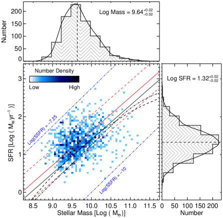
Figure 2: SFR versus stellar mass for SFGs at 2 $<$ $z$ $<$ 2.5 in VUDS. The full sample has median stellar mass of 10^9.64 $\sim$ 4$\times$10⁹ M_⊙ and median SFR of 10^1.32 $\sim$ 20 M_⊙ per year. The quoted uncertainties are the errors on the median ($1.253\,\times\,\sigma/\sqrt{\rm N_{\rm gal}}$) estimated from the 1$\sigma$ dispersion of the distribution and the total number of galaxies, where $\pm$1$\sigma$ corresponds to the range between the 16th and the 84th percentile values of the distribution. The black solid curve is the KDE of the distribution. The black solid line shows the main sequence of SFGs as defined by Daddi et al. (2007) at $z$ $\sim$ 2, and the solid red line is the best-fit relation (with the slope fixed to the value from Daddi et al.) for our sample with the total scatter ($\sim$0.4 dex) shown by red dashed lines. The black dashed line is the main sequence relation from Whitaker et al. (2014), while the black dot-dashed line is the relation from Schreiber et al. (2015). The blue dot-dashed lines show limits on SSFR for these galaxies. The density of points is color-coded as shown in the color-bar.

3 UV Spectral Slope ($\beta$)

The UV spectral slope ($\beta$) is determined from a power-law fit to the UV continuum spectrum (Calzetti et al., 1994), $f_{\lambda}$ $\varpropto$ $\lambda^{\beta}$, where $f_{\lambda}$ is the flux density per unit wavelength (ergs s^-1 cm^-2 Å^-1). We use the VUDS spectra of SFGs at 2 $<$ $z$ $<$ 2.5 to estimate their UV slope by fitting a linear relation to the full wavelength range between rest-frame 1400 and 2400Å in the observed (Log($\lambda$) versus Log( $f_{\lambda}$)) spectrum. The rest-frame wavelength range (1400–2400Å) includes 7 out of 10 spectral fitting windows identified by Calzetti et al. (1994) to estimate the UV spectral slope for local starburst galaxies, and takes full advantage of the spectral coverage of the VUDS spectra at these redshifts. Figure 3 shows four examples of UV spectral slope fitting on the VUDS spectra. Before fitting, the spectra were cleaned by masking out known lines and removing any spurious noise spikes. The fitting was done using the IDL routine LINFIT, which fits the data to the linear model by minimizing the $\chi^{2}$ statistic. The running dispersion values measured on the clean spectra are used as measured errors, and the routine uses these errors to compute the covariance matrix. In Figure 3, the solid red line is the best-fit spectroscopic slope while dashed red lines show 1$\sigma$ uncertainties associated with the best-fit relation. The formal statistical uncertainty in the best-fit $\beta_{\rm spec}$, which is measured over a large number of points, is smaller than the uncertainty in photometric $\beta$ measured using few photometric points. For comparison, we also measure the UV spectral slope directly from the broad-band photometry which encompasses a similar rest-frame wavelength range. We used $BVRI$ bands for the ECDFS field, $g^{+}Vr^{+}i^{+}$ for the COSMOS field, and $g^{\prime}r^{\prime}i^{\prime}z^{\prime}$ bands for the VVDS field. These photometric bands cover a rest-frame wavelength range from $\sim$1200Å to $\sim$3000Å, depending on the redshift. Figure 3 also shows the photometric magnitudes of the broad-band filters which are used to measure the photometric UV slope, and the corresponding best-fit photometric UV slope. Figure 4 shows the UV spectral slope ($\beta$) distribution as measured from the VUDS spectra ($\beta_{\rm spec}$) and the broad-band photometry ($\beta_{\rm phot}$). The median $\beta_{\rm spec}$ is –1.36 $\pm$ 0.02, and the median $\beta_{\rm phot}$ is –1.32 $\pm$ 0.02. The quoted uncertainties are the errors on the median ($1.253\,\times\,\sigma/\sqrt{\rm N_{\rm gal}}$). It is worth noting that even if we use two or three photometric bands, covering the similar wavelength range as four bands, we get similar median values for the photometric UV slope of the whole sample, which is in the range of –1.40$\pm$0.10. We also measured UV slopes by convolving the spectra with the photometric filter curves, and found that the median value is –1.31 $\pm$ 0.03, which is very similar to the median photometric and spectroscopic UV slopes.

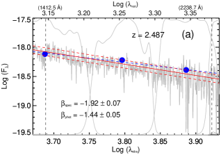
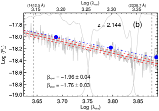
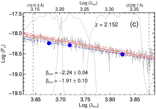
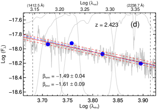
Figure 3: Examples of UV spectral slope ($\beta$) fitting on the VUDS spectra (shown in grey). The spectra between rest-frame 1400Å to 2400Å (between dashed vertical lines) are fitted with a linear relation (solid red lines) between Log($\lambda$) vs Log(F_λ) after masking out known lines and removing spurious noise spikes. The dashed red lines are 1$\sigma$ deviations in the best-fit relation. The blue filled circles are the photometric magnitudes from the broad-band filters (grey curves) used to measure the photometric $\beta$, while the blue dashed line is a linear fit between these photometric data points to estimate the photometric UV slope.

In Figure 4 , and in subsequent figures of this paper, we will calculate statistical significance for the distributions and correlations in the following two ways: (a) for histograms, we use KS-statistics on the distributions. The probability of KS-statistics (P_KS) measures whether two sets of data are drawn from the same parent distribution or not. Small values (close to zero) of P_KS show that the cumulative distribution functions of the two sets of data are significantly different. This is measured using the IDL routine KSTWO, and (b) for correlations, we use the Spearman correlation test. Values of the Spearman correlation coefficient ($\rho$) close to $\pm$1 imply strong monotonic correlation, while values close to 0 imply no significant correlation between two variables. The significance level is denoted by P_SC, where small values of P_SC imply significant correlation. It is important to note that for a large sample size, very small differences (or small $\rho$ values) in two sets of data will be detected as highly significant. When a statistic is significant, it simply means that the difference is real. It does not mean the difference is large or important. The Spearman correlation coefficient is measured using the IDL routine R_CORRELATE, and is measured from all galaxies as well as from the median-binned values.This routine can also give the value of the sum-squared difference of ranks, and the number of standard deviations ($\sigma$) by which it deviates from its null-hypothesis expected value.

In Figure 4 (left panel), the median values of $\beta_{\rm spec}$ and $\beta_{\rm phot}$ are very similar and differ by only $\sim$0.04. This difference is not significant considering that the errors on the median values is $\pm$0.02. However, the full distributions of $\beta_{\rm spec}$ and $\beta_{\rm phot}$ are marginally different as confirmed by P_KS $\sim$ 0.00057, which implies that a null hypothesis (similar distributions) is rejected at $\sim$3$\sigma$ level. To investigate the difference between individual $\beta_{\rm spec}$ and $\beta_{\rm phot}$, we look at four examples shown in Figure 3. Figure 3(a) shows an extreme example in which the difference between two $\beta$s is $\sim$0.5, though $\beta_{\rm phot}$ is within the 1$\sigma$ uncertainties of $\beta_{\rm spec}$. Figure 3(b) and Figure 3(c) show examples where $\beta_{\rm phot}$ is just outside the 1$\sigma$ uncertainties in $\beta_{\rm spec}$ and we find that both these $\beta$ values differ by $\sim$0.2-0.3. Figure 3(d) shows an example where the difference between the two $\beta$s is very small ($\sim$0.1) and well within the measurement uncertainties.

The middle panel of Figure 4 shows the direct comparison between individual $\beta_{\rm spec}$ and $\beta_{\rm phot}$, while the bottom plot in the middle panel shows the difference between $\beta_{\rm spec}$ and $\beta_{\rm phot}$ as a function of $\beta_{\rm spec}$. The best orthogonal fit relation between $\beta_{\rm spec}$ and $\beta_{\rm phot}$ is flatter than 1-to-1 relation, and is given by $\beta_{\rm phot}=-0.43+0.63\times\beta_{\rm spec}$. The total scatter in the $\beta_{\rm spec}$ vs $\beta_{\rm phot}$ relation could be as high as $\sim$0.5. The uncertainties in both $\beta$ measurements could be the main cause of the flatter slope ($<$ 1) and the large scatter. The average measurement error in $\beta_{\rm spec}$ is $\sim$0.08, while it is $\sim$0.15 for $\beta_{\rm phot}$. Depending on the object and its redshift, it is possible to have additional factors affecting $\beta$ measurements of individual galaxies, as discussed below.

For $\beta_{\rm spec}$, there are two potential sources of uncertainties. First, the bluest part of the spectra is sensitive to various atmospheric and galactic corrections made to the spectra (see Le Fèvre et al., 2015; Thomas et al., 2014, for details), and even though these corrections are carefully applied to minimize the flux loss, there are uncertainties in the bluest part of the spectra. The UV slope measurement is sensitive to the changes in the anchor blue region of the spectra and hence, this could affect the UV slope measurements for some objects. Second, as seen in Figure 3(a), the spectroscopic $\beta$ is fitted in such a way that it avoids the more noisy red part of the spectrum to minimize its effect on the best-fit slope, which could make $\beta_{\rm spec}$ steeper or bluer compared to $\beta_{\rm phot}$. While this fitting effect is kept at the minimum level, any small difference in the fitting of the red part of the spectrum could lead to slightly bluer $\beta_{\rm spec}$ compared to $\beta_{\rm phot}$. These uncertainties in $\beta_{\rm spec}$ are estimated to be small ($\lesssim$0.1) but could vary from object to object.

For $\beta_{\rm phot}$, the wavelength range over which $\beta$ is measured has a great influence on the resulting $\beta$ values. Calzetti et al. (1994) defined a wavelength baseline (1250Å to 2600Å) to measure $\beta$ for galaxies at lower redshifts and this range is widely used for all measurements. But as discussed in Calzetti (2001), the UV slopes fitted with the longer wavelength baseline are always bluer (more negative) compared to the UV slopes from shorter baseline (see also Meurer et al., 1999; Talia et al., 2015). The main reason is that the slopes fitted with the longer wavelength baseline cover the 2300-2800Å range which has a large decrement due to a large number of closely spaced FeII absorption lines and this low continuum gives them steeper/bluer slopes. Our $\beta_{\rm phot}$ is measured using broad photometric bands, and depending on the exact redshift of a galaxy the wavelength range covered by these bands could be as large as $\sim$1200Å to $\sim$3000Å. This range includes the wavelength range (1400Å to 2400Å) used to measure $\beta_{\rm spec}$, but $\beta_{\rm phot}$ has a longer wavelength baseline for many galaxies which could lead to bluer $\beta_{\rm phot}$ for these galaxies. The other factor affecting the $\beta_{\rm phot}$ measurement is the contribution of strong Ly$\alpha$ emission to the flux of the bluest band used for measuring $\beta_{\rm phot}$. For a small number of strong Ly$\alpha$ emitters, it is likely that the bluest band used in the $\beta_{\rm phot}$ measurement is affected by the strong Ly$\alpha$ emission line. To check this effect, we measured $\beta$s for galaxies with no Ly$\alpha$ emission and for galaxies with strong Ly$\alpha$ emission. We find that the difference between the median values of $\beta_{\rm phot}$ and $\beta_{\rm spec}$ is smaller ($\beta_{\rm spec}$ bluer by $\sim$0.05) for galaxies with no Ly$\alpha$ emission compared to galaxies with strong Ly$\alpha$ emission, where on average $\beta_{\rm phot}$ is bluer compared to $\beta_{\rm spec}$ by $\sim$0.13. Hence, strong Ly$\alpha$ line in the bluest photometric band could lead to higher flux in that band which in turn could give steeper/bluer $\beta_{\rm phot}$. This is confirmed by our estimation of Ly$\alpha$ contamination to the bluest photometric band by comparing flux densities with and without Ly$\alpha$ line in the broadband. We found that the contamination in the broadband for the strongest Ly$\alpha$ emission lines could be $\sim$0.05–0.1 mag. This difference in the magnitude of bluest band could cause $\sim$0.1–0.2 difference in the photometrically measured UV slope. These uncertainties in $\beta_{\rm phot}$ are estimated to be $\lesssim$0.2, but could vary from object to object.

In summary, the average $\beta_{\rm spec}$ and $\beta_{\rm phot}$ are very similar for the VUDS SFG sample, and the uncertainties discussed above could affect individual measurements, as shown in the middle panel of Figure 4. The detailed comparison between individual $\beta$s, and quantifying various sources of uncertainties for such a large sample, requires an in-depth study, which is beyond the scope of this paper.

The median $\beta_{\rm spec}$ value of the whole SFG sample, –1.36$\pm$0.02 with 1$\sigma$ scatter of $\sim$0.5, is consistent with the UV slope estimates obtained at similar redshifts using ground-based spectra. Talia et al. (2012) obtained $\beta_{\rm spec}$ of –1.11$\pm$0.44 (rms) for 74 SFGs at $z$ $\simeq$ 2 using VLT/FORS2 spectra, while Noll & Pierini (2005) used FORS spectroscopic data of 34 UV-luminous galaxies at 2 $<$ $z$ $<$ 2.5 and found $\beta_{\rm spec}$ for the sub-sample of galaxies to be –1.01$\pm$0.11. Both these $\beta$ values are roughly consistent with our median $\beta_{\rm spec}$ when considering the additional uncertainty introduced by the fact that both studies used slightly different wavelength range ($\sim$1200-2600Å, and $\sim$1200-1800Å, respectively), from each other & our own, to fit the UV slope. In addition, the median photometric UV slope obtained here, –1.32$\pm$0.02 with 1$\sigma$ scatter of $\sim$0.5, is very similar to the average UV slopes measured at these redshifts (2 $<$ $z$ $<$ 2.5) from HST photometry (e.g., –1.58$\pm$0.27 (1$\sigma$) from Bouwens et al. 2009 and –1.71$\pm$0.34 (1$\sigma$) from Hathi et al. 2013). These $\beta$ values — spectroscopic and photometric — are also in good agreement with the evolution of $\beta$ with redshift which shows that the average $\beta$ at 2 $<$ $z$ $<$ 2.5 is redder compared to $\beta$ at higher redshifts (e.g., Hathi et al., 2008b; Bouwens et al., 2009; Finkelstein et al., 2012).

3.1 $\beta$ versus E_s(B–V)

The UV radiation is absorbed by dust and heated dust particles re-emit absorbed energy in the mid- and far-infrared. The ratio of L_IR-to-L_UV is the direct measure of dust attenuation in a galaxy. A higher L_IR/L_UV ratio implies a larger dust content. There is an excellent correlation between L_IR/L_UV and the UV spectral slope at $z$ $\sim$ 2 (e.g., Seibert et al., 2002; Reddy et al., 2012), which is in good agreement with the local measurements (e.g., Meurer et al., 1997, 1999), in that, an increase in L_IR/L_UV corresponds to redder UV slopes. For SFGs at 2 $<$ $z$ $<$ 2.5 in the VUDS sample, the correlation between the UV slope and SED derived E_s(B–V) is shown in Figure 4 (right panel). A positive correlation is observed between $\beta$ and E_s(B–V) implying redder UV slope for dustier (higher E_s(B–V)) galaxies. We show the correlation of E_s(B–V) with both, photometric and spectroscopic, $\beta$s. The statistical significance of this correlation is measured by the Spearman correlation test. The Spearman correlation coefficient ($\rho$) is 0.25 (0.95) for all (binned) $\beta_{\rm spec}$ values and 0.65 (1.00) for all (binned) $\beta_{\rm phot}$ values, which implies high significance (P_SC $\sim$ 0) for a strong positive correlation. The significance of $\rho$ as measured by the number of standard deviations by which the sum-squared difference of ranks deviates from its null-hypothesis expected value is $\sim$7$\sigma$ for all $\beta_{\rm spec}$ values and $\sim$18$\sigma$ for all $\beta_{\rm phot}$ values. The correlation between $\beta_{\rm phot}$ and E_s(B–V) is stronger, in part, because they are both estimated from the same photometry. The $\beta_{\rm spec}$ correlation is flatter compared to the $\beta_{\rm phot}$ correlation, which means that galaxies with bluer $\beta$ have lower E_s(B–V) for $\beta_{\rm phot}$, and galaxies with redder $\beta$ have higher E_s(B–V) for $\beta_{\rm phot}$, compared to $\beta_{\rm spec}$. Also, it should be noted that within the large 1$\sigma$ scatter in the E_s(B–V) values, the difference between these two $\beta$s is not large in all UV slope bins. The corresponding A₁₆₀₀ (the dust absorption at 1600Å) in Figure 4 (right panel) is estimated from E_s(B–V) using the Calzetti law (A₁₆₀₀ $\sim$ 10$\times$E_s(B–V); Calzetti et al., 2000). We have added best-fit relations from three different studies (Talia et al., 2015; Oteo et al., 2014; Buat et al., 2012). The Oteo et al. (2014) relation is for galaxies at $z$ $\sim$ 2, while the Buat et al. (2012) relation is for galaxies at 1 $\lesssim$ $z$ $\lesssim$ 2. The Talia et al. (2015) relation covers a larger redshift range, 1 $<$ $z$ $<$ 3. We do not see any trend (with redshift) between these relations and ours. Our relation is flatter compared to their relations and the difference is largest at redder UV slopes. This difference between our relation and theirs could be due to the sample of SFGs used in these studies. All these studies use UV+FIR selected galaxies which are primarily dusty galaxies with FIR detection in 24$\mu$m and/or Herschel observations, while we do only UV selection and do not require FIR detection for our sample. This means that our sample does not include most of the dusty galaxies at these redshifts, which would make this relation much steeper with larger E(B–V) values and redder UV slopes. Talia et al. (2015) finds that the differences in various samples could also lead to a large dispersion ($\sim$0.7) in the dust-UV slope relation. Our future studies will specifically look at IR/FIR detections for these galaxies to investigate their dust properties.

In the remaining sections of this paper we use the spectroscopic UV slope and refer to $\beta_{\rm spec}$ as $\beta$, unless stated otherwise. We are using $\beta_{\rm spec}$ in this paper because they have smaller measurement uncertainties, and the trends/relations explored in this paper are very similar for both spectroscopic and photometric UV slopes.

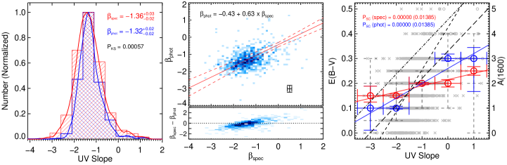
Figure 4: (Left) UV spectral slope ($\beta$) distribution as measured from the VUDS spectra (red histogram) and the broad-band photometry (blue histogram). The solid curve is the KDE of the distribution. The median $\beta$ values as well as KS-test probability (P_KS) show very small difference in these $\beta$s. (Middle) $\beta_{\rm spec}$ versus $\beta_{\rm phot}$. The solid red line is the best orthogonal fit relation between these two $\beta$s, while the dashed lines show the uncertainties in the best-fit relation. This figure also shows the difference ($\beta_{\rm spec}$-$\beta_{\rm phot}$) as a function of $\beta_{\rm spec}$. The dotted line is for $\beta_{\rm spec}$-$\beta_{\rm phot}$ = 0. The density of points is color-coded as in previous figures. Average uncertainties in these measurements are plotted in the bottom-right corner. (Right) The correlation between the UV slope and the SED derived E_s(B–V) is such that the redder UV slope implies dustier [higher E_s(B–V)] galaxies. The error bars in x illustrate the sizes of the bins, while the errors in y are $\pm$1$\sigma$ scatter (dashed error bars) corresponding to the range between the 16th and the 84th percentile values within each bin, while the smaller solid error bars are the errors on the median values ($1.253\,\times\,\sigma/\sqrt{\rm N_{\rm gal}}$). The red circles are for the spectroscopic $\beta$, while the blue circles are for the photometric $\beta$. The black small-dashed line is the dust-UV slope relation at 1 $\lesssim$ $z$ $\lesssim$ 2 from Buat et al. (2012), the black dot-dashed line is the dust-UV slope relation at $z$ $\sim$ 2 from Oteo et al. (2014), and the black long-dashed line is the dust-UV slope relation at 1 $<$ $z$ $<$ 3 from Talia et al. (2015). The background grey points are the values for all galaxies (crosses are $\beta_{\rm spec}$ and open circles are $\beta_{\rm phot}$). The statistical significance from the Spearman correlation coefficient is shown to confirm the correlation. The corresponding A₁₆₀₀ (shown on the right y-axis) is estimated from E_s(B–V) using the Calzetti law (A₁₆₀₀ $\sim$ 10$\times$E_s(B–V); Calzetti et al., 2000).

3.2 $\beta$ versus M₁₅₀₀

A color-magnitude relation has previously been observed at various redshifts. The interpretation of this relation depends on which color is used. If the color is between the rest-frame UV and the rest-frame optical (e.g., Papovich et al., 2004) and spans the 4000Å/Balmer break, then it is strongly dependent on the stellar population age, while if the color is blue-ward of the 4000Å break (e.g., Finkelstein et al., 2012) then it is more sensitive to the dust extinction than age. Here we use rest-frame UV colors (i.e., UV spectral slope, $\beta$) to infer the color-magnitude relation for SFGs at 2 $<$ $z$ $<$ 2.5. Figure 5 shows the spectroscopic UV slope versus UV absolute magnitude (M₁₅₀₀). We estimate the slope, $d\beta/dM_{\rm 1500}$, by fitting a linear model to the median-binned values, $\beta=a+d\beta/dM_{\rm 1500}\times\ M_{\rm 1500}$. We find the best-fitting solution to be $d\beta/dM_{\rm 1500}$ = 0.00$\pm$0.04. Essentially no correlation of $\beta$ with absolute magnitude is observed, which could imply that $\beta$ does not change with UV luminosity for $\sim$L^∗ galaxies. The Spearman correlation coefficient ($\rho$) is 0.18 (-0.4) for all (binned) M₁₅₀₀–$\beta$ values, which implies no correlation at a high significance (P_SC = 0.60). The $\rho$ for all galaxies shows high significance (P_SC ¡ 10^-3) for a strong correlation but it is misleading as it is strongly affected by a small number of galaxies with significant redder UV slope.

Various studies have investigated the color-magnitude relation at high redshifts ($z$ $\gtrsim$ 2), and the results are inconclusive. Reddy et al. (2008) found weak-to-no correlation between dust or UV color (related as shown in Figure 4) and $R$ mag for UV-selected galaxies at 1.5 $\lesssim$ $z$ $\lesssim$ 2.6. Similarly, Heinis et al. (2013) through their investigation of far-infrared/dust properties of UV selected galaxies at $z$ $\sim$ 1.5 found that the average UV slope is mostly independent of the UV luminosity. On the other hand, Bouwens et al. (2009) studied the relation between the UV slope and $M_{UV}$ for a sample of $U$-band dropout galaxies at $z$ $\simeq$ 2.5 and found a positive color-magnitude correlation. At higher redshifts ($z$ $>$ 3), similar disagreements have been observed for samples based on the Lyman break color selection, in the sense that, some studies find no (or very weak) trends between $\beta$ and UV magnitude (e.g., Ono et al., 2010; Finkelstein et al., 2012; Dunlop et al., 2012; Castellano et al., 2012), while other studies find a strong color-magnitude relation (e.g., Wilkins et al., 2011; Bouwens et al., 2012; Rogers et al., 2014; Bouwens et al., 2014). Bouwens et al. (2014) also argue that this relation could be described by a double power-law with a different slope for fainter magnitudes. The differences in these various studies could be due to many systematic and/or physical reasons, such as selection of galaxy samples (especially at lower redshifts), UV magnitude and/or $\beta$ measurements, intrinsic scatter in $\beta$, dynamic range in UV luminosity. Our study relies on a UV selected sample with spectroscopic redshifts but it lacks a significant dynamic range in UV luminosity as seen in Figure 5. A detailed study of a uniformly selected spectroscopic sample covering a large range in UV luminosity is needed to understand the true nature of the color-magnitude relation at high redshifts. At least for $\sim$L^∗ ($\sim$0.5L^∗ – 3.0L^∗) galaxies in a uniformly selected VUDS sample at 2 $<$ $z$ $<$ 2.5 there appears to be no correlation between $\beta$ and M₁₅₀₀.

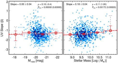
Figure 5: Spectroscopic UV slope versus the UV absolute magnitude (left) and the stellar mass (right). The density of points is color-coded as in previous figures, while the red open circles are the median-binned values for these parameters. The error bars in x illustrate the sizes of the bins, while the errors in y are $\pm$1$\sigma$ scatter (dashed error bars) corresponding to the range between the 16th and the 84th percentile values within each bin, while smaller solid error bars are the errors on the median values ($1.253\,\times\,\sigma/\sqrt{\rm N_{\rm gal}}$). The dashed red lines show the best-fit linear relations. We find no correlation (slope = 0.00$\pm$0.04) of $\beta$ with the UV absolute magnitude, while we see a positive correlation (slope = 0.18$\pm$0.04) of $\beta$ with the stellar mass (redder UV slope for higher mass galaxies). The statistical significance from the Spearman correlation coefficient is shown to confirm these results.

3.3 $\beta$ versus Stellar Mass

The relation between $\beta$ and M₁₅₀₀ could be affected by the biases and/or differences in the way different authors measure and define M₁₅₀₀ (e.g., Finkelstein et al., 2012). On the other hand, there is a well known correlation between M₁₅₀₀ and the stellar mass such that, stellar mass increases as brightness increases (e.g., Stark et al., 2009; Sawicki, 2012; Hathi et al., 2013), which we can exploit to better understand the dependence of $\beta$ on M₁₅₀₀. Therefore, we can compare $\beta$ to the stellar mass as an alternate way to explore the dependence of $\beta$ on M₁₅₀₀. Figure 5 shows the correlation between the spectroscopic UV slope and the stellar mass (M_∗). We estimate the slope, $d\beta/dLog(M_{*})$, by fitting a linear model to the median-binned values, $\beta=a+d\beta/dLog(M_{*})\times\ Log(M_{*})$. We find the best-fitting solution to be $d\beta/dLog(M_{*})$ = 0.18$\pm$0.04. A stronger correlation of $\beta$ with stellar mass is observed compared to the $\beta$–M₁₅₀₀ correlation, which suggests a redder UV slope (more dust) for massive star-forming galaxies. This is not necessarily surprising as star-formation generally increases with stellar mass in star-forming samples and in turn, the dust content generally increases with increasing star-formation (e.g., Lemaux et al., 2014b). The Spearman correlation coefficient ($\rho$) is 0.11 (1.0) for all (binned) M_∗-$\beta$ values, which implies high significance (P_SC $\sim$ 10^-3) for a strong positive correlation. A similar trend between $\beta$ and stellar mass is also observed at $z$ $\gtrsim$ 4.0 (e.g., Finkelstein et al., 2012).

The VUDS survey targets star-forming galaxies brighter than $i_{AB}$ $\sim$ 25 mag, so there are survey limitation/incompleteness given the limited area of the survey, in the sense that, we do not target many high mass galaxies (Log(M_∗) $\gtrsim$ 10.5), and we miss many fainter star-forming galaxies with lower stellar masses (Log(M_∗) $\lesssim$ 9.0) because of the magnitude limit. These survey limitations affect the range in stellar mass range probed in our study, and hence, could impact the exact nature of our $\beta$-stellar mass correlation. An extensive study covering a large mass range is required to fully understand this M_∗–$\beta$ correlation.

The M₁₅₀₀–$\beta$ and M_∗–$\beta$ correlations are similar if we use $\beta_{\rm phot}$ instead of $\beta_{\rm spec}$. For $\beta_{\rm phot}$, the linear slope values for the M₁₅₀₀–$\beta$ and M_∗–$\beta$ relations are 0.01$\pm$0.05 and 0.32$\pm$0.05, respectively.

4 SFGs with and without Ly$\alpha$ Emission

The galaxies selected by their (strong) Ly$\alpha$-emission, are becoming an important probe of galaxy formation, cosmic reionization, and cosmology. Ly$\alpha$ emission is an important diagnostic of physical processes in star forming galaxies, in particular at cosmological distances, since Ly$\alpha$ becomes the strongest emission line in the UV-optical window at redshifts $z$ $>$ 2.0. These galaxies — because of their observed physical properties at higher redshifts — are thought to be the progenitors of present-day Milky Way type galaxies (e.g., Gawiser et al., 2007), though dissimilar results from various Ly$\alpha$ studies at different redshifts amplify the importance to better understand these galaxies. The SFG population in our sample is divided into Ly$\alpha$ emitters and non-emitters based on their rest-frame Ly$\alpha$ EW.

The Ly$\alpha$ EWs for VUDS SFGs were measured as described in Cassata et al. (2015). To summarize, we measured EWs of the Ly$\alpha$ line manually using the IRAF splot tool, while the uncertainties in EW were estimated using the formalism from Tresse et al. (1999). The median EW uncertainty varies as a function of the EW from $\pm$5Å (for weak absorbers and emitters) to $\pm$25Å (for strong absorbers and emitters). We first put each galaxy spectrum in its rest-frame based on the spectroscopic redshift. Then, two continuum points bracketing Ly$\alpha$ are manually marked and the rest-frame EW is measured for emission as well as the absorption lines. The line is not fitted with a Gaussian, but the flux in the line is determined by simply summing the pixels in the area covered by the line and the continuum. This method allows the measurement of lines with asymmetric shapes (i.e., with deviations from Gaussian profiles), which is the shape observed for most Ly$\alpha$ lines. The interactive method also allows us to control the level of the continuum, taking into account defects that may be present around the line. This approach produces more reliable and accurate measurements compared to an automated ‘impartial’ measurement because the visual inspection is capable of accounting for the complex nature of the Ly$\alpha$ emission/absorption line.

Figure 6 shows the rest-frame EW distribution for the Ly$\alpha$ line. Here, positive EWs are emission lines, while negative EWs are for absorption lines. We divide the SFG population into three sub-groups based on their Ly$\alpha$ EW. The galaxies that show no Ly$\alpha$ in emission (EW $\leq$ 0Å) are defined as SFG_N, while the galaxies with Ly$\alpha$ in emission, irrespective of its strength (EW $>$ 0Å), are defined as SFG_L. The third group is for strong Ly$\alpha$ emitters (EW $\geq$ 20Å) called LAEs. The number of galaxies with Ly$\alpha$ EW $\geq$ 20Å is 87 and this number drops to 27 for galaxies with EW $\geq$ 50Å. Such a distribution is partially due to the fact that our sample does not select most of the galaxies with very high EW (EW $\gtrsim$ 50Å), whose continuum is usually very faint ($\sim$27 mag) and which are usually detected in NB imaging/emission-line selected surveys. This selection effect means that we are probing Ly$\alpha$ emitting galaxies with brighter continuum compared to galaxies selected based on NB/emission-line surveys. We also show the distribution of Ly$\alpha$ luminosities, L(Ly$\alpha$), for SFG_L and LAEs in the middle panel of Figure 6. The median L(Ly$\alpha$) of the SFG_L sample is $\sim$10⁴⁰ ergs/s, while the median L(Ly$\alpha$) of the LAE sample is $\sim$10⁴¹ ergs/s. The LAEs discovered in the VUDS survey are significantly less luminous than the Ly$\alpha$ emitters found by most NB/emission-line surveys ($\sim$10⁴² ergs/s) at similar redshifts (e.g., Guaita et al., 2010; Hagen et al., 2014). The fraction of LAEs as a function of redshift is shown in the right panel of Figure 6. Approximately 10% of SFGs at these redshifts are strong Ly$\alpha$ emitters, consistent with previous Ly$\alpha$ studies at $z$ $\simeq$ 2 (e.g., Reddy et al., 2008), and in agreement with the general scenario that the number of LAEs increases as redshift increases reaching $\sim$30-40% at $z$ $\simeq$ 6 (e.g., Stark et al., 2010; Curtis-Lake et al., 2012; Cassata et al., 2015).

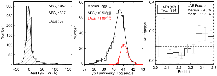
Figure 6: (Left) Rest-frame EW distribution for SFGs with Ly$\alpha$ in emission (positive EWs) and Ly$\alpha$ in absorption (negative EWs). The vertical dashed line indicates EW = 20Å, the adopted lower limit in Ly$\alpha$ EW for LAEs (or strong Ly$\alpha$ emitters). The solid curve is the KDE of the distribution. (Middle) Distribution of Ly$\alpha$ luminosities for the SFG_L (black) and the LAE (red) samples. The KDE of the distribution is shown by a solid curve. (Right) Fraction of LAEs as a function of redshift for our sample. Approximately 10% of SFGs at these redshifts are strong Ly$\alpha$ emitters, consistent with previous Ly$\alpha$ studies (e.g., Reddy et al., 2008; Cassata et al., 2015) at similar redshifts.

The composite spectra of the SFG_N, SFG_L, and LAE samples are shown in Figure 7. They are generated by stacking the rest-frame shifted individual spectra which are rebinned to dispersion of 2Å per pixel (2Å $\sim$ 5Å/(1+$z$), where $\sim$5Å is the native pixel scale of the LR Blue grism in the observed frame), and then the entire spectrum is normalized to the mean flux in the wavelength range of 1350–1450Å before taking the median value of all galaxies in the composite at each wavelength. Figure 7 shows the most prominent emission and absorption lines, whose detailed analysis will be conducted in a future paper. Here, it is worth pointing out that the median UV spectral slope (between 1400-2400Å) does not show any appreciable difference among these three sub-samples as shown in the bottom panel of Figure 7.

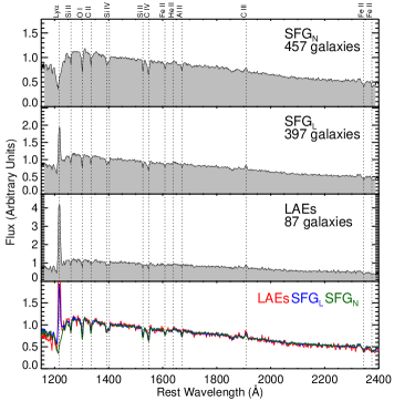
Figure 7: Stacked (median-combined) rest-frame UV spectra for SFG_N, SFG_L, and LAEs. The strong absorption and emission features are marked by the vertical dotted lines. The SFG_N spectrum shows strong absorption lines (Si, C, O, Fe, Al), but these absorption lines get weaker with increasing strength of Ly$\alpha$-emission. The bottom panel shows similarity in the spectroscopic UV slope for these samples.

The galaxies with strong Ly$\alpha$ in emission, usually selected using NB imaging or serendipitous spectroscopy, show different physical properties compared to galaxies with no Ly$\alpha$ in emission or LBGs (e.g., Gawiser et al., 2006, 2007; Lai et al., 2008; Cassata et al., 2011). These two galaxy populations (LAEs and LBGs) are selected differently so the differences seen when comparing the two populations are mainly due to selection effects. Here, we use a UV-selected sample (selected based on UV continuum/magnitude) to investigate stellar population differences between Ly$\alpha$ emitting galaxies and non-Ly$\alpha$ emitting galaxies. A common selection for Ly$\alpha$ emitters as well as non-emitters could reveal real intrinsic differences between these two classes of objects. Figure 8 shows the comparison between SFG_N, SFG_Land LAEs. The total number of galaxies identified as SFG_L and SFG_N is large enough (457 SFG_N, 397 SFG_L, 87 LAEs) to get robust statistics. On average, SFG_L (and LAEs) are less dusty, and have lower SFR compared to SFG_N. These differences are small, but they are significant because of the large sample used in this study. To understand the significance of these differences we use KS-statistics on these distributions. The P_KS $\sim$ 10^-4 value for E_s(B–V) and SFR distributions implies that the null hypothesis (similar distributions) is rejected at $>$99.9% or $>$3$\sigma$ level. The differences in stellar mass, SSFR, M₁₅₀₀, and $\beta_{\rm spec}$ for SFG_N and SFG_L/LAEs are not statistically significant (i.e., the null hypothesis is rejected only at $\lesssim$2.5$\sigma$ level). It is important to note that the KS-test does not consider errors/uncertainties in two quantities while comparing their distributions. We tested the robustness of these results by constructing 100 bootstrap samples by randomly extracting values from the confidence intervals of the best-fit stellar parameters. We re-ran the KS test on each of these 100 artificial samples with a goal to compare the stellar population parameters of the LAE and non-LAE populations. For E_s(B–V) and SFR, a null hypothesis was consistently ruled out at $\sim$3$\sigma$ level, while for other parameters, the null hypothesis rejection is at much lower significance ($\lesssim$2$\sigma$). We also compare the median values of the best-fit stellar parameters for LAEs and non-LAEs, and we find similar significance for the median values of E_s(B–V), SFR, and other parameters in these bootstrap samples. These artificial samples show that even when accounting for the uncertainty in best-fit parameters, a significant difference exists for E_s(B–V) and SFR, such that galaxies with Ly$\alpha$ emission tend to be less dusty, and lower in SFR than galaxies with weak or no Ly$\alpha$ emission.

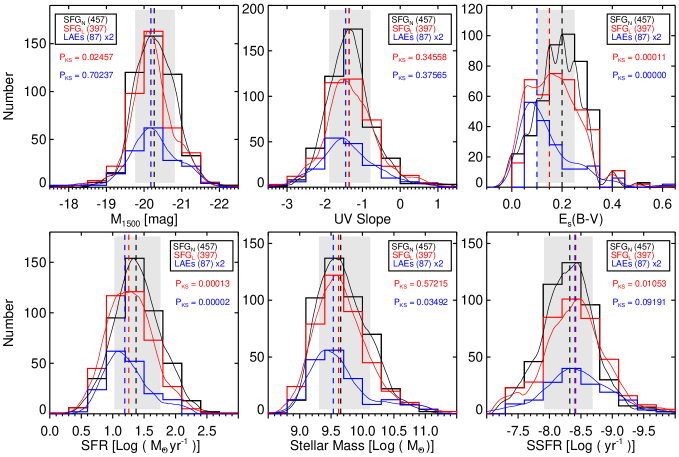
Figure 8: Comparison between SFG_N (black histograms), SFG_L (red histograms), and LAEs (blue histograms) as a function of stellar parameters. The total number of galaxies identified as SFG_N, SFG_L, and LAEs are shown in the legend. The median value of the distribution is indicated by a vertical dashed line. The solid curves are KDE of the distribution. The grey shaded regions cover $\pm$1$\sigma$ dispersion/scatter, which corresponds to the range between the 16th and the 84th percentile values, of the SFG_N distribution. The statistical significance based on the KS test (red for SFG_L, and blue for LAEs with respect to SFG_N) is shown to confirm any correlation.

Table 1 summarizes average spectral and photometric properties of our SFG_N, SFG_L, and LAE samples. Our results show that SFG_L (and LAEs) have — on average — lower dust content than SFG_N. The differences in these two samples is statistically significant based on the K-S test results (P_KS $\sim$ 10^-4), which says that distributions of E_s(B–V) are different for SFG_N and SFG_L. Though the difference in the distributions of these populations is statistically significant, the difference between their median values is small as shown in Table 1. The median E_s(B–V) values for SFG_L or LAEs and SFG_N differ only by $\sim$0.05 or $\sim$0.1 (i.e., by a factor of $\sim$1.3 or 2) which is smaller than or similar to the 1$\sigma$ scatter in these distributions ($\sim$0.1). This small difference in the dust content of SFG_N and SFG_L or LAE galaxies is consistent, within the large scatter, with the small difference in the median values of $\beta_{\rm spec}$, and a small difference in $\beta_{\rm phot}$ values ($\sim$0.1-0.2) between these populations. Such a small difference between the E_s(B–V) values for SFG_L or LAEs and SFG_N is also consistent with the observations at higher redshifts. Pentericci et al. (2010) found small differences between E_s(B–V) values for their samples of LBG_N and LBG_L at $z$ $\sim$ 3. A similar study at $z$ $\sim$ 4 by Pentericci et al. (2007) agrees with this E_s(B–V) trend for galaxies with and without Ly$\alpha$ in emission.

Table 1: Average properties of SFG_N, SFG_L, and LAEs derived from the SED-fitting

Parametersa	SFGNb	SFGLc	LAEsd
Ngal	457	397	87
M1500 (mag)	–20.27${}^{+0.03\;(0.50)}_{-0.03\;(0.55)}$	–20.18${}^{+0.03\;(0.43)}_{-0.04\;(0.57)}$	–20.18${}^{+0.07\;(0.54)}_{-0.10\;(0.78)}$
M2300 (mag)	–20.56${}^{+0.03\;(0.45)}_{-0.03\;(0.55)}$	–20.45${}^{+0.03\;(0.36)}_{-0.04\;(0.55)}$	–20.46${}^{+0.05\;(0.38)}_{-0.09\;(0.66)}$
Ly$\alpha$ Luminosity (Log [erg/s])	—	40.53${}^{+0.03\;(0.52)}_{-0.05\;(0.75)}$	41.09${}^{+0.06\;(0.41)}_{-0.04\;(0.31)}$
UV slope (spectroscopic)	–1.35${}^{+0.03\;(0.56)}_{-0.03\;(0.53)}$	–1.36${}^{+0.04\;(0.66)}_{-0.03\;(0.52)}$	–1.45${}^{+0.10\;(0.80)}_{-0.07\;(0.58)}$
UV slope (photometric)	–1.30${}^{+0.03\;(0.45)}_{-0.02\;(0.35)}$	–1.35${}^{+0.04\;(0.59)}_{-0.03\;(0.41)}$	–1.58${}^{+0.11\;(0.85)}_{-0.04\;(0.30)}$
Es(B–V) (mag)	0.20${}^{+0.00\;(0.05)}_{-0.01\;(0.10)}$	0.15${}^{+0.01\;(0.10)}_{-0.01\;(0.10)}$	0.10${}^{+0.02\;(0.15)}_{-0.01\;(0.05)}$
SFRSED (Log [$M_{\odot}\cdot yr^{-1}$])	1.37${}^{+0.02\;(0.39)}_{-0.02\;(0.34)}$	1.26${}^{+0.02\;(0.36)}_{-0.02\;(0.34)}$	1.19${}^{+0.05\;(0.40)}_{-0.04\;(0.28)}$
SFRUV (Log [$M_{\odot}\cdot yr^{-1}$])	1.23${}^{+0.03\;(0.56)}_{-0.03\;(0.57)}$	1.19${}^{+0.04\;(0.59)}_{-0.04\;(0.60)}$	0.99${}^{+0.12\;(0.91)}_{-0.09\;(0.65)}$
Mass (Log [$M_{\odot}$])	9.65${}^{+0.03\;(0.47)}_{-0.02\;(0.34)}$	9.62${}^{+0.03\;(0.46)}_{-0.02\;(0.36)}$	9.54${}^{+0.08\;(0.62)}_{-0.04\;(0.33)}$
SSFR (Log [$yr^{-1}$])	–8.32${}^{+0.02\;(0.41)}_{-0.02\;(0.36)}$	–8.42${}^{+0.03\;(0.46)}_{-0.03\;(0.44)}$	–8.41${}^{+0.06\;(0.43)}_{-0.08\;(0.59)}$

Figure 8 also shows that SFG_L (and LAEs) have — on average — lower SED-based SFRs than SFG_N. The KS test results show that distributions of the SFG_L and SFG_N samples are significantly different i.e., P_KS $\sim$ 10^-4, which is as significant as the E_s(B–V) comparison. The median SFR for the SFG_L or LAE sample from the SED-fitting technique is 10^1.26 $\sim$ 18 M_⊙ yr^-1 or 10^1.19 $\sim$ 15 M_⊙ yr^-1, while the median SFR for the SFG_N sample is 10^1.37 $\sim$ 23 M_⊙ yr^-1. Therefore, the median SFR values for SFG_L or LAEs and SFG_N differ only by a factor of $\sim$1.3 or 1.5, which is much smaller in comparison to the 1$\sigma$ scatter of these distributions ($\sim$0.4 dex or a factor of $\sim$2). To assess the effect of SED-fitting parameters on the SFRs (e.g., Kusakabe et al., 2015), we also compute SFR using the UV luminosity (M₁₅₀₀) corrected for the dust using the $\beta$–A₁₆₀₀ relation from Meurer et al. (1999). The median values for the UV-based SFRs (SFR_UV) are shown in Table 1 and they are very similar to the SED-based SFRs. The median SFR_UV for the SFG_L or LAE sample is 10^1.19 $\sim$ 15 M_⊙ yr^-1 or 10^0.99 $\sim$ 10 M_⊙ yr^-1, and for the SFG_N sample is 10^1.23 $\sim$ 17 M_⊙ yr^-1. Therefore, the difference between SFR_UV values of these two populations is very small and agrees very well with the difference quoted for the SED-based SFRs. This is consistent with the fact that the UV absolute magnitudes (M₁₅₀₀) of galaxies with and without Ly$\alpha$ in emission are very similar as shown in the Table 1. This result is consistent with similar studies at $z$ $\sim$ 3–4 (e.g., Pentericci et al., 2007, 2010).

Figure 8 does not show any significant difference between the median values of stellar mass ($\sim$0.1 dex or a factor of $\sim$1.2). This result is in contrast to higher redshift studies at $z$ $\sim$ 3–4 (e.g., Pentericci et al., 2007, 2010), where they find that galaxies without Ly$\alpha$ in emission are more massive (by a factor of $\sim$2–5) compared to galaxies with Ly$\alpha$ in emission. The difference between these studies could be due to the sample selection, in that the stellar mass probed in those studies by the galaxies at $z$ $\sim$ 3–4 are much lower (down to $\sim$10⁸ M_⊙) compared to the VUDS sample (down to $\sim$10⁹ M_⊙). The lowest mass regime at $z$ $\sim$ 3–4 is mostly populated by galaxies with Ly$\alpha$ in emission which results in this large difference in stellar masses for Ly$\alpha$ emitters and non-emitters at these redshifts. We do not probe this low mass regime between 10⁸ and 10⁹ M_⊙ at 2 $<$ $z$ $<$ 2.5 because of our continuum magnitude limit of $i_{AB}$ $\lesssim$ 25 mag. Therefore, we conclude that, within the luminosities probed by VUDS, we do not see any significant difference between the stellar mass of galaxies with and without Ly$\alpha$ in emission. We will investigate any redshift evolution in these correlation in our future VUDS studies, which will extend these measurements to higher redshifts ($z$ $\gtrsim$ 3).

5 Ly$\alpha$ EW and Stellar Population Properties

To further investigate properties of SFG_N and SFG_L, we explore the correlation between the rest-frame Ly$\alpha$ EW and stellar population parameters, such as M₁₅₀₀, UV slope, E_s(B–V), SFR, stellar mass, and SSFR. Figure 9 shows the correlation between Ly$\alpha$ EW and best-fit SED/spectral parameters. It should be noted that the Spearman correlation is measured from all galaxies as well as from the median-binned values. The E_s(B–V) and SFR show moderate-to-weak monotonic correlation ($\rho$ $\sim$ –0.2 and P_SC ¡ 10^-4) with Ly$\alpha$ EW. The significance of $\rho$ as measured by the number of standard deviations by which the sum-squared difference of ranks deviates from its null-hypothesis expected value is $\sim$5$\sigma$ for all E_s(B–V) values and $\sim$6$\sigma$ for all SFR values. The stellar mass, M₁₅₀₀, and $\beta$ show much weaker correlation with EW ($\rho$ $\lesssim$ 0.1). The significance of $\rho$ as defined above is $\lesssim$3$\sigma$ for all values of these parameters. The trends observed between the best-fit stellar parameters and EWs are in general agreement with the median values of the stellar parameters obtained from the distributions of SFG_N and SFG_L in Figure 8.

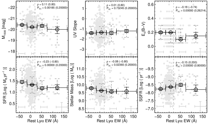
Figure 9: Correlation between rest-frame Ly$\alpha$ EW and best-fit stellar population parameters. The vertical dashed line indicates EW = 20Å, the adopted lower limit in Ly$\alpha$ equivalent width for LAEs. The size of the last bin is increased with respect to that of the other bins to increase the number of galaxies in that bin. The light grey points are individual measurements while the black circles are binned medians. The error bars in x illustrate the sizes of the bins, while the errors in y are $\pm$1$\sigma$ scatter (dashed error bars) corresponding to the range between 16th and the 84th percentile values within each bin, while smaller solid error bars are the errors on the median values ($1.253\,\times\,\sigma/\sqrt{\rm N_{\rm gal}}$). The statistical significance from the Spearman correlation coefficient for all galaxies (median-binned values) is shown to confirm these correlations. Average uncertainties in these measurements are plotted in the bottom-right corner. The median uncertainties in the EW measurement varies as a function of EW as shown by different x error bars.

With increasing rest-frame Ly$\alpha$ EW, we see a weak but significant trend in that, galaxies are less dusty, and less star-forming, as indicated by a decrease in SFR by about $\sim$0.2 dex from non-LAEs to LAEs. While the average EW varies from –38.0Å to 120Å, the median E_s(B–V) decreases from 0.20 to 0.15, the median SFR_SED decreases from 28 M_⊙ yr^-1 to 16 M_⊙ yr^-1, the median stellar mass decreases from 6.2$\times$10⁹ M_⊙ to 3.9$\times$10⁹ M_⊙, and the median SSFR decreases from 5.9$\times$10^-9 yr^-1 to 6.3$\times$10^-9 yr^-1. All these differences in stellar parameters as a function of Ly$\alpha$ EW are small compared to the scatter observed in each EW bin, as measured by 1$\sigma$ dispersion (see Figure 9).

These results demonstrate that there is a statistically significant correlation between Ly$\alpha$ EW and stellar parameters, such as SFR and E_s(B–V), while no significant correlations are found for stellar mass, M₁₅₀₀, and $\beta$. The differences we observe are small compared to the large scatter in their distributions. This outcome is true whether or not we focus on all galaxies with Ly$\alpha$ in emission or only strong Ly$\alpha$ emitters (LAEs). This is in contrast with results from NB or emission-line selected LAE studies (e.g., Gawiser et al., 2006, 2007; Lai et al., 2008; Guaita et al., 2011; Hagen et al., 2014). These studies find lower dust, lower stellar mass and higher SSFR for galaxies with strong Ly$\alpha$ in emission. The LAE samples used in these emission-line/NB-selected surveys have Ly$\alpha$ luminosities in the range of $\sim$10⁴² ergs/s, which is an order of magnitude more luminous than VUDS LAEs, as shown in Figure 6. It is also worth emphasizing that VUDS is a UV continuum selected survey and galaxies are targeted based on their photometric redshifts and not on the strength of the Ly$\alpha$ line. We have 27 galaxies beyond rest-frame Ly$\alpha$ EW = 50Å, so by selection, our sample does not include extremely low mass ($\sim$10⁸ M_⊙) galaxies usually selected from emission-line/NB techniques. Moreover, among the emission-line/NB-selected LAEs, those that have lower Ly$\alpha$ luminosities, have similar SFR as normal star-forming galaxies but lie on the lower mass end of the star-forming main sequence (e.g., Kusakabe et al., 2015). Hence, the difference in the sample selection could play a significant role in such a comparison as we could be comparing two intrinsically different populations of galaxies.

The comparison of stellar population properties of galaxies with and without Ly$\alpha$ emission has also been done on UV-selected galaxies at $z$ $\simeq$ 2 and higher, and our results are broadly consistent with the literature. Pentericci et al. (2010) found weak/no correlation between SFRs of galaxies with and without Ly$\alpha$ emission at $z$ $\simeq$ 3 but we find a correlation (with a small difference in SFR) possibly because of the large statistics in the VUDS sample. With a smaller number of galaxies (130) in the Pentericci et al. sample such a detection was difficult to observe. Our finding of a very small decrease in the SED-based dust content (i.e., E_s(B–V)) of these two populations agrees well with the Pentericci et al. (2010) study. At $z$ $\simeq$ 3, Kornei et al. (2010) find that LAEs have lower E_s(B–V) and SFRs compared to non-LAEs. The difference in these two stellar population parameters for LAEs and non-LAEs, as found by Kornei et al., is much larger than what we observe, but show similar decreasing trends in these two quantities. This trend of lower dust and SFR for strong Ly$\alpha$ emitters has also been observed at $z$ $\simeq$ 2 by Reddy et al. (2006). The study of Kornei et al. (2010) agrees well with our result that there is no significant difference between stellar masses of LAEs and non-LAEs. Therefore, based on the comparison between SFG_L/LAEs and SFG_N, as well as Ly$\alpha$ EW correlations with stellar parameters, we suggest that our LAE sample shows a small decrease in E_s(B–V) and SFR but otherwise their stellar populations are not very different from the galaxies that do not show Ly$\alpha$ in emission.

Lai et al. (2008) studied NB-selected LAEs at $z$ $\simeq$ 3 by dividing them into Spitzer/IRAC-detected (brighter than m_3.6 = 25.2 mag) and IRAC-undetected (fainter than m_3.6 = 25.2 AB mag) samples. They found that IRAC-undetected LAEs were less massive and younger compared to IRAC-detected LAEs, concluding that IRAC-detected LAEs are a more evolved population similar to brighter/massive UV-selected LAEs (e.g., Shapley et al., 2001, 2003). To investigate this trend for VUDS LAEs, we examined our LAEs as a function of magnitude in the Spitzer/IRAC 3.6$\mu$m band. We find that 74% of SFG_N, 66% of SFG_L, and 53% of LAEs have detections in the Spitzer/IRAC 3.6$\mu$m band down to $\sim$25 mag. The LAE fraction with IRAC detection in our sample is much larger than the $\sim$30% found in Lai et al. (2008), which is a direct consequence of the difference in the sample selection between the two studies. The NB-selected LAEs typically have very faint continuum in all optical and NIR bands as they are mostly lower mass/younger galaxies compared to normal star-forming galaxies. IRAC-detection is only possible in NB-LAEs if they host more evolved population which makes continuum brighter in the red bands. We do not expect many NB-selected LAEs to be more evolved/massive and brighter in IRAC bands, therefore their IRAC-detected fractions are more likely to be small compared to other star-forming galaxies. A similar study at $z$ $\simeq$ 2 (Guaita et al., 2011), also found that $\sim$25% of NB-selected LAEs had IRAC detection down to m_3.6 $\sim$ 24.5 AB mag. We find a higher detection rate (51%) of IRAC-detected LAEs in our sample using the same limiting magnitude of 24.5 mag as Guaita et al. Figure 10 shows the comparison of IRAC-detected and IRAC-undetected galaxies in all three samples as a function of stellar mass, and SFR. The stellar mass correlations show that, in all three samples, IRAC-detected galaxies are more massive than IRAC-undetected galaxies. These correlations are statistically significant based on their P_KS values $<$ 10^-2. We do not see any significant correlation for SFR in all three samples, both in terms of P_KS and their median values.

These comparisons show that the VUDS LAE sample has a larger fraction of galaxies with IRAC detection compared to NB-selected LAEs at $z$ $\simeq$ 2–3, and that IRAC-detected LAEs are more likely to host evolved populations compared to IRAC-undetected LAEs. A large fraction of UV-selected LAEs have similar masses as SFG_N galaxies but with lower SFRs suggesting that these LAEs host more evolved populations. The low fraction of IRAC detection in NB-selected LAEs implies that these galaxies are less evolved compared to UV-selected LAEs.

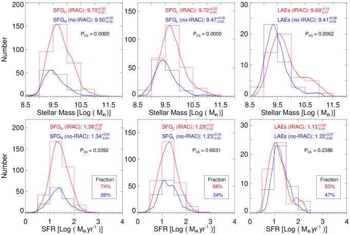
Figure 10: Comparison between Spitzer/IRAC 3.6$\mu$m-detected (red; brighter than m_3.6 $\sim$ 25 mag) and IRAC-undetected (blue; fainter than m_3.6 $\sim$ 25 mag) galaxies as function of stellar mass and SFR for SFG_N, SFG_L, and LAEs. The fraction of galaxies detected/un-detected in IRAC are shown in the legend. The solid curve is the KDE of the distribution. The statistical significance based on the KS test is shown to confirm the observed correlation.

6 Results and Discussion

We use a large spectroscopic sample of 854 SFGs at 2 $<$ $z$ $<$ 2.5 from VUDS to investigate their spectral and photometric properties. The VUDS spectra were used to measure the UV spectral slope and Ly$\alpha$ EW. The SED fitting on multi-wavelength photometric data using Le PHARE provided best-fitting stellar parameters, such as stellar mass, M₁₅₀₀, E_s(B–V), SFR, and SSFR. The VUDS observations extend to a fairly large area of $\sim$1 deg², which implies that our sample spans a large range in SFR ($\sim$3-150 M_⊙ yr^-1) and stellar mass ($\sim$5$\times$10⁸ to 10¹¹ M_⊙). The VUDS 2 $<$ $z$ $<$ 2.5 sample covers a substantial range in UV absolute magnitude around M^∗ ($\pm$1 mag), the characteristic magnitude at these redshifts. We divide SFGs into three sub-groups, SFG_N, SFG_L and LAEs, based on their rest-frame Ly$\alpha$ EW. We find that the fraction of LAEs is $\sim$10% at these redshifts, which is consistent with previous studies (e.g., Reddy et al., 2008), and is in accordance with the general picture where the Ly$\alpha$ fraction increases with redshift (e.g., Stark et al., 2010; Curtis-Lake et al., 2012; Cassata et al., 2015). The Ly$\alpha$ fraction apparently starts to decrease at higher redshift ($z$ $\gtrsim$ 6.5; e.g., Pentericci et al., 2011), where large amounts of neutral hydrogen start to affect the visibility of Ly$\alpha$ line indicating the onset of the reionization epoch.

The UV spectral slope $\beta$ can be used to derive the dust attenuation for local starburst galaxies (e.g., Calzetti et al., 1994; Leitherer et al., 1999) and has been adopted as a dust indicator for high redshifts galaxies (e.g., Noll et al., 2004; Hathi et al., 2008b; Finkelstein et al., 2012; Bouwens et al., 2014). The main reason is that the intrinsic UV slope depends only weakly on metallicity and stellar populations for star-forming galaxies (e.g., Heckman et al., 1998; Leitherer et al., 1999). In addition, $\beta$ shows a strong correlation with the L_IR-to-L_UV ratio, a standard dust indicator (e.g., Meurer et al., 1999; Reddy et al., 2010). On average, the spectroscopic UV slope for SFGs at 2 $<$ $z$ $<$ 2.5, measured using VUDS spectra, is comparable to the photometric $\beta$ measured using multiple photometric bands, and have smaller measurement uncertainties. The measured UV slope — spectroscopic and photometric — is in accordance with the evolutionary trend of $\beta$ with redshift, which shows that lower redshift galaxies have, on average, redder UV slope compared to higher redshift galaxies (e.g., Bouwens et al., 2012; Hathi et al., 2013). With dust being the major factor influencing the UV slope, this implies that lower redshift galaxies have more dust compared to higher redshift galaxies. We use the spectroscopic $\beta$ measurements to explore its correlation with M₁₅₀₀ and stellar mass. Comparing $\beta$ to the stellar mass we find a significant correlation, in the sense that massive galaxies are redder, which is in general agreement with the higher redshift measurements of Finkelstein et al. (2012). We find no correlation between M₁₅₀₀ and $\beta$. This result is at variance with what found by some authors at higher redshifts (e.g., Bouwens et al., 2012; Rogers et al., 2014), but it is similar to other studies which do not find any significant correlation between $\beta$ and M₁₅₀₀ (e.g., Finkelstein et al., 2012; Castellano et al., 2012; Heinis et al., 2013). It is vital to note that this correlation could be affected by the biases and/or differences in the way different authors measure M₁₅₀₀ and/or $\beta$ but most importantly the dynamic range in M₁₅₀₀ plays a crucial role. Extensive studies exploring a larger range in M₁₅₀₀ and stellar masses and investigating different biases in these correlations will shed more light on the true nature of these relations and provide a better physical understanding.

There are several studies investigating the stellar population of UV-selected LAEs at $z$ $\simeq$ 2–3 (e.g., Shapley et al., 2001, 2003; Erb et al., 2006; Reddy et al., 2008; Kornei et al., 2010). We find that LAEs in our sample have lower dust content, lower SFR and lower SSFR compared to non-emitters. These differences are very small compared to the large scatter in these SED-based parameters but they are significant because of the large sample size. Shapley et al. (2001) and Kornei et al. (2010) found that LAEs at $z$ $\simeq$ 3 have lower SFRs, lower dust and lower SSFR compared to LBGs, which is consistent with our observed trends, but we find much smaller differences in these stellar parameters for our galaxies. We find only weak or no correlation of stellar mass with Ly$\alpha$ EW for a sample with median Log(M_∗) = 9.64 and median Log(SFR) = 1.32. Kornei et al. (2010) studied a large ($\sim$300) sample of UV-selected galaxies, with and without Ly$\alpha$ emission, with a median stellar mass of Log(M_∗) = 9.92 and a median SFR of Log(SFR) = 1.57, both slightly higher than for our sample. They found that there is no significant difference in the stellar mass between these two populations in accordance with our weak-to-no correlation of stellar mass with the Ly$\alpha$ EW. The results obtained here show no strong correlation or large differences between stellar parameters as a function of the Ly$\alpha$ EW, which is consistent with the small sample study of Reddy et al. (2008) using UV-selected galaxies at $z$ $\simeq$ 2–3. It is clear that the properties of galaxies with and without Ly$\alpha$ in emission are pretty similar suggesting that the two populations, at least for typical ($\sim$L^∗) galaxies and to the level of detail we are able to probe, are roughly comprised of similar galaxies. Erb et al. (2006) used composite spectra of UV-selected LAEs and non-LAEs at $z$ $\simeq$ 2 and found that galaxies with strong Ly$\alpha$ EW had lower stellar masses. Our results on SFR and dust are broadly consistent with previous studies, but the lack of a strong correlation between stellar mass and EW needs to be explored with a sample that spans a larger dynamic range in stellar mass as lower mass galaxies could strongly impact the stellar mass correlation between Ly$\alpha$ emitters and non-emitters.

In comparison to UV-selected LAEs, LAEs selected based on the emission-line/NB technique at $z$ $\simeq$ 2 and beyond have very low masses $\sim$10⁸ M_⊙ compared to $\sim$10¹⁰ M_⊙ for non-LAEs (e.g., Gawiser et al., 2007; Finkelstein et al., 2007; Lai et al., 2008; Guaita et al., 2011; Vargas et al., 2014). Also, these LAEs are much more luminous in Ly$\alpha$ ($\sim$10⁴² ergs/s) than VUDS LAEs, which are on average an order of magnitude less luminous ($\sim$10⁴¹ ergs/s). We do not find such low mass, high Ly$\alpha$ luminosity LAEs in our sample mainly because these strong emitters have low continuum luminosities and are not selected by the VUDS magnitude selection. In fact, such galaxies would be missed in almost all UV continuum selected samples (e.g., Shapley et al., 2001; Reddy et al., 2008; Kornei et al., 2010), as emission-line/NB LAEs probe a different luminosity range compared to magnitude-limited samples. However, Kornei et al. (2010) have argued that when NB-selected LAEs are restricted to luminosities probed by continuum selected samples, both samples are statistically very similar, which is consistent with the result put forward by the study of Verhamme et al. (2008), where bright NB-selected LAEs represent the same population as continuum selected LAEs. Therefore, UV-selected LAEs and NB-selected LAEs need to probe similar luminosities for proper comparison between these two populations.

In the literature there are two possible scenarios under which galaxies emit Ly$\alpha$ during the evolution process. Studies of faint NB-selected LAEs (e.g., Gawiser et al., 2006, 2007; Lai et al., 2008) have argued that LAEs represent the beginning of an evolutionary sequence of galaxy formation. According to these studies, the main reason behind this argument is that LAEs have lower dust content, lower stellar mass, younger stellar ages, and higher SSFRs compared to non-LAEs which means that LAEs are building up their stellar mass at a faster rate than non-LAEs through mergers and/or star-formation episodes. On the other hand, studies of brighter continuum selected LAEs (e.g., Shapley et al., 2001, 2003; Kornei et al., 2010) have suggested that LAEs represent a later stage in the evolutionary sequence. These studies argue that LAEs have lower dust content, lower SFR, older stellar ages, and lower SSFRs compared to non-LAEs which means that LAEs are more quiescent than non-LAEs. This could be the result of strong outflows from supernovae and massive star winds, which expel both gas and dust from a young, dusty non-LAE. These arguments raise a question: are these two scenarios two different phases of the evolution process or do these two possibilities describe a single phase? Lai et al. (2008) investigated the stellar populations of 162 NB-selected LAEs at $z$ $\simeq$ 3.1 by dividing them in two groups based on their Spitzer/IRAC flux. They find that $\sim$70% of the LAEs are undetected in 3.6$\mu$m down to 25.2 mag. Based on their stacking analysis, they find a clear difference between these two divided samples. The average stellar population of the IRAC-undetected sample had an age of $\sim$200 Myr and a mass of $\sim$3$\times$10⁸ M_⊙, consistent with the scenario that LAEs are mostly young and low-mass galaxies. On the other hand, the IRAC-detected LAEs were on average significantly older and more massive, with an average age of $\sim$1 Gyr and mass of $\sim$10¹⁰ M_⊙. The stellar populations of the IRAC-detected sample of Lai et al. (2008) are very similar to those of continuum selected brighter LAEs (e.g., Shapley et al., 2001, 2003; Kornei et al., 2010). Similar results are also found in the study of Guaita et al. (2011) at $z$ $\simeq$ 2.1, in that, the fraction of IRAC-detected LAEs is $\sim$25% down to 24.5 mag and these galaxies are more massive/evolved than those that are faint in IRAC. We find larger fraction of IRAC-detected LAEs ($\sim$50%) compared to NB-selected LAEs ($\sim$30%) at $z$ $\simeq$ 2–3, which could imply that UV-selected LAEs are more evolved compared to NB/emission-line selected LAEs. Also, the IRAC-detected LAEs have higher stellar mass, similar to IRAC-detected non-LAEs, but with lower SFR which is consistent with the more evolved nature of these galaxies. The scenario in which LAEs are more evolved than non-LAEs is plausible if strong outflows in non-LAEs destroy or remove dust and gas from the galaxies, allowing Ly$\alpha$ photons to escape. Our results from direct comparison of galaxies with and without Ly$\alpha$ emission show small differences in stellar populations, such that galaxies with Ly$\alpha$ emission have lower SFR and dust content than non-Ly$\alpha$ emitting galaxies. This result broadly agrees with previous studies involving UV-selected galaxies at $z$ $\simeq$ 3 (e.g., Shapley et al., 2003; Kornei et al., 2010), though we observe small difference between physical parameters of Ly$\alpha$ emitters and non-emitters. Past studies of LAEs (e.g., Verhamme et al., 2008; Nilsson et al., 2011; Acquaviva et al., 2012), suggest that LAEs have a large range in stellar population properties implying that a strong LAE phase either is a long duration phase ($\sim$1 Gyr; Lai et al., 2008) or is recurring in SFGs.

Studies focusing on comparing stellar populations of galaxies with and without Ly$\alpha$ emission have shown that various effects, including the sample selection, continuum and Ly$\alpha$ luminosities, measurements of stellar parameters, and SED fitting assumptions play an important role in how we compare Ly$\alpha$ emitters and non-emitters. It is also essential to understand that these comparisons and correlations are not universal and could change with redshift. Extending these studies to higher redshifts, where the fraction of Ly$\alpha$ emitters increases, is essential to generate a self-consistent picture of how LAEs and non-LAEs form and evolve. In future studies, we will extend such an analysis to $z$ $\simeq$ 3–6 using the VUDS data, to better understand how these LAE properties/trends evolve with redshift from $z$ $\sim$ 6 to $z$ $\sim$ 2.

7 Summary

In this paper, we have investigated the spectro-photometric properties of a large sample of SFGs at 2 $<$ $z$ $<$ 2.5 that were selected from the VIMOS Ultra-Deep Survey in the ECDFS, COSMOS, and VVDS fields. These galaxies were targeted because of their photometric redshifts, and are therefore UV continuum-selected galaxies. The VUDS spectra were used to measure the UV spectral slope ($\beta$) and Ly$\alpha$ EWs, while we used deep multi-wavelength observations in these extensively observed fields to derive physical parameters (stellar mass, SFR, E_s(B–V), M₁₅₀₀, SSFR) from the SED fitting process. We compared Ly$\alpha$ emitters and non-emitters using these parameters and also explored correlations of these parameters with Ly$\alpha$ EW. Our results can be summarized as follows:

$\bullet$ We obtain reliable measurements of spectroscopic UV slopes, which are — on average — similar to the photometric measurements of $\beta$, and have smaller measurement uncertainties. The median values of $\beta_{\rm spec}$ and $\beta_{\rm phot}$ are consistent with each other and with the general picture in which UV slopes get redder with decreasing redshift, implying higher dust content at lower redshifts. We find a significant correlation between $\beta$ and SED-based dust indicator E_s(B–V). We observe no correlation between $\beta$ and M₁₅₀₀, while a strong correlation between $\beta$ and stellar mass is observed. These results are consistent with higher redshift observations.

$\bullet$ For a proper comparison, we divide these SFGs into three subgroups based on their EWs: SFG_N (EW $\leq$ 0Å), SFG_L (EW $>$ 0Å), and LAEs (EW $\geq$ 20Å). The LAEs make up $\sim$10% of the total SFG sample at 2 $<$ $z$ $<$ 2.5, which is consistent with previous observations.

$\bullet$ We find that at 2 $<$ $z$ $<$ 2.5, within the luminosities probed, the SFG_L (and LAE) sample has slightly lower E_s(B–V) and SFRs compared to the SFG_N sample. These differences are small but statistically significant. It is important to note that we are able to probe these small differences in physical parameters because of our large SFG sample. We do not find any or find weaker significant differences in stellar mass, M₁₅₀₀, and $\beta$ for these two samples. We find similar results when we compare Ly$\alpha$ EW and physical parameters. These results indicate that the properties of galaxies with and without Ly$\alpha$ in emission are remarkably similar suggesting that the two populations, at least for typical ($\sim$L^∗) galaxies and to the level of detail we are able to probe, are roughly comprised of similar galaxies.

$\bullet$ When we divide the LAEs based on their Spitzer/IRAC 3.6$\mu$m magnitudes, the fraction of IRAC-detected LAEs ($\sim$50%) is much greater than the fraction of IRAC-detected NB-selected LAEs ($\sim$30%) at $z$ $\simeq$ 2–3. This could imply that UV-selected LAEs host a more evolved stellar population compared to NB/emission-line selected LAEs. Based on differing stellar population results for LAEs at various redshifts, we cannot rule out multiple or recurring Ly$\alpha$ emitting phases for SFGs.

Future studies of higher redshift ($z$ $\simeq$ 3–6) galaxies from VUDS, where the fraction of Ly$\alpha$-emitting galaxies increases substantially, will help us to better understand the LAE population at these redshifts, as well as to see how these correlation evolve with redshift.