Origin of structure: Statistical characterization of the primordial density fluctuations and the collapse of the wave function

Abstract

The statistical properties of the primordial density perturbations has been considered in the past decade as a powerful probe of the physical processes taking place in the early universe. Within the inflationary paradigm, the properties of the bispectrum are one of the keys that serves to discriminate among competing scenarios concerning the details of the origin of cosmological perturbations. However, all of the scenarios, based on the conventional approach to the so-called “quantum-to-classical transition” during inflation, lack the ability to point out the precise physical mechanism responsible for generating the inhomogeneity and anisotropy of our universe starting from and exactly homogeneous and isotropic vacuum state associated with the early inflationary regime. In past works, we have shown that the proposals involving a spontaneous dynamical reduction of the quantum state provide plausible explanations for the birth of said primordial inhomogeneities and anisotropies. In the present manuscript we show that, when considering within the context of such proposals, the characterization of the spectrum and bispectrum turn out to be quite different from those found in the traditional approach, and in particular, some of the statistical features, must be treated in a different way leading to some rather different conclusions.

I Introduction

Recent advances in observational cosmology are allowing a detailed testing of our understanding of the early universe. In particular, the inflationary paradigm, considered as a one of the most important cornerstones of modern cosmology, is regarded as providing an explanation for the origin of cosmological structure mukhanov1990 ; hawking1982 ; starobinsky1982 ; guth1982 ; halliwell1985 ; mukhanov1992 . Indeed, recent observational data (e.g. WMAP wmap9 , SDSS sdss9 , Planck planck ), is in very good agreement with the theoretical predictions offered by the inflationary paradigm. According to this theory, the generation of the primordial inhomogeneities, constituting “the seeds of galaxies,” is also rather image-evoking: The perturbations start as quantum fluctuations of the inflaton field, and as the universe goes trough an era of accelerated expansion, the physical wavelength associated with the perturbations is stretched out reaching cosmological scales.

At this point one is led to treat the quantum fluctuations as classical density perturbations; there are several kinds of arguments for such consideration. However, in most of the original works mentioned above, the issue is only dealt implicitly; meanwhile, in more recent works, such as Albrecht ; Polarski , specific arguments have been put forward based on the highly squeezed nature of the field’s quantum state, or on detailed decoherence arguments. Finally, the traditional picture states that these classical perturbations continue evolving into the cosmic structure responsible for galaxy formation, stars, planets and eventually life and human beings.

However, as has been discussed at length in previous works, the complete theory must not only allow one to find expressions that are in agreement with observations, but also, be able to provide an explanation of the precise physical mechanism behind its predictions. As originally discussed in sudarsky2006 , there is a conceptual difficulty in the standard explanation for the birth of cosmic structure provided by inflation: The issue is that according to this account, and starting from a highly homogeneous and isotropic state that characterizes the background inflaton and space-time, as well as the quantum state of the perturbations, the universe must end in a state with “actual” inhomogeneities and anisotropies. Let us be a bit more explicit and recall that, when considering quantum mechanics as a fundamental theory applicable, in particular, to the universe as a whole, then one must regard any classical description of the state of any system as a sort of imprecise characterization of a complicated quantum mechanical state. The universe that we observe today is clearly well described by an inhomogeneous and anisotropic classical state; therefore, such description must be considered as an imperfect description of an equally inhomogeneous and anisotropic quantum state. Consequently, if we want to consider the inflationary account as providing the physical mechanism for the generation of the seeds of structure, such account must contain an explanation for why the quantum state that describes our actual universe does not possess the same symmetries as the early quantum state of the universe, which happened to be perfectly symmetric (the symmetry being the homogeneity and isotropy). As there is nothing in the dynamical evolution (as given by the standard inflationary approach) of the quantum state that can break those symmetries, then we are left with an incomplete theory. In fact, this shortcoming has been recognized by others in the literature Padmanabhan ; Mukhanov ; Weinberg ; Lyth .

The detailed discussion of the conceptual problems associated with the inflationary paradigm, and the proposed paths for resolution of the issue within schemes following standard Quantum Mechanics (e.g., the decoherence program, many-worlds interpretation and the consistent histories approach), have been discussed in detail by some of us and by others in susana2013 ; pearle2007 ; sudarsky2006 ; sudarsky2009 . We will not reproduce those arguments here and invite the interested reader to consult those references; the above paragraph is meant only to provide the reader with a brief indication of the kinds of issues that a detailed analysis of such questions involves.

The idea that has been presented in previous works sudarsky2006 ; sudarsky2006b ; sudarsky2007 ; sudarsky2009 ; sudarsky2011 , as a possibility to deal with the aforementioned problem, relies on supplementing the standard inflationary model with an hypothesis involving the modification of quantum theory so as to include a spontaneous dynamical reduction of the quantum state (sometimes referred as the self-induced collapse of the wave function) and to consider such reduction as an actual physical process; taking place independently of observers or measuring devices. Regarding the situation at hand, the basic scheme is the following: A few $e$-folds after inflation has started, the universe finds itself in an homogeneous and isotropic quantum state, then during the inflationary regime a quantum collapse of the wave function is triggered (by novel physics that could possibly be related to quantum gravitational effects), breaking in the process the unitary evolution of quantum mechanics and also, in general, the symmetries of the original state. In our situation the post-collapse state will not in general be isotropic nor homogeneous. This state is moreover assumed to be sufficiently peaked in the relevant variables so as to be susceptible to an approximate classical characterization describing a universe that includes the inhomogeneities and anisotropies. That classical description will continue to evolve following the standard physical processes of post-inflationary cosmology, into the universe we have today.

The idea of modifying quantum mechanics by incorporating a self-induced collapse is not a new idea First Collapse and there has been a considerably amount of research along this lines: The continuous spontaneous localization (CSL) model pearle1989 , representing a continuous version of the Ghirardi-Rimini-Weber (GRW) model ghirardi1985 , and the ideas of Penrose penrose and Diósi diosi regarding gravity as the main agent responsible for the collapse, are among the main programs proposed to describe the physical mechanism of a self-induced collapse of the wave function. For more recent examples see Refs. weinberg2011 ; bassi2003 . In fact, the implications of applying the CSL model to the inflationary scenario have been studied in Refs. pedro ; jmartin and tpsingh leading to interesting results constraining the parameters of the model in terms of the parameters characterizing the inflationary model.

On the other hand, the statistical analyses in Refs. adolfo ; susana2012 show how the predictions of the simple collapse schemes, used in previous works, can be confronted with recent data from the Cosmic Microwave Background (CMB), including the 7-yr release of WMAP wmap7 and the matter power spectrum measured using LRGs by the Sloan Digital Sky Survey sdssb . In fact, results from those analyses indicate that while several schemes or “recipes” for the collapse are compatible with the observational data, others are not, allowing to establish constraints on the free parameters of the schemes. Those works serve to underscore the point that, in addressing the conceptual issues confronting the inflationary paradigm, one is not only dealing with “philosophical issues,” but that these have impact in the theoretical predictions. While, at the same time, the conclusions drawn can lead to important insights, as well as a better understanding of the nature of those predictions and novel ways to consider the relation between such predictions and the observations.

In this work, we will be primarily concerned with the characteristics of the “primordial bispectrum” although we will also make some interesting observations regarding the primordial spectrum itself. In the inflationary paradigm, the primordial bispectrum has been regarded as one of the indicators characterizing possible primordial “non-Gaussianities.” By non-Gaussianity, one generically refers to any deviations in the observed fluctuations from the random field of linear, Gaussian, curvature perturbations. It is commonly believed that the study of non-Gaussianities will play a leading role in furthering our understanding of the physics of the very early universe that created the primordial seeds for large-scale structures komatsu2009 . As a matter of fact, the shape and amplitude of the bispectrum is currently being used in order to discriminate among various inflationary models. The amplitude of non-Gaussianities is characterized in terms of a dimensionless parameter $f_{\textrm{NL}}$ (defined in Sec. IV). Distinct models of inflation predict different values for $f_{\textrm{NL}}$. The amount of non-Gaussianity from simple inflationary models, which are based on a single scalar filed with slow-roll inflationary regime, is expected to be very small salopek1990 ; salopek1991 ; falk1992 ; gangui1993 ; acquaviva2002 ; maldacena2002 ; however, a very large class of more general models, such as those with multiple scalar fields, special features in the inflaton potential, non-canonical kinetic terms, deviations from Bunch-Davies vacuum, and others (see Ref. bartolo2004 and references therein for a review ), are thought to be able to generate substantially higher levels of non-Gaussianity.

In this article, we will consider the simplest slow-roll inflation model, within the approach involving the hypothesis of “the collapse of the wave function.” We will focus on the simplest collapse scheme involving a single instantaneous collapse per mode proposal, although several of the results will be valid in more general schemes. We will also use some previous results alberto ; sigma , which indicate that certain intrinsic non-linearities associated with the collapse of the wave function in a gravitational context, generically induce correlations between the random variables characterizing the collapse of the wave function in the different modes. In other words, the collapse of the wave function, cannot operate in an exactly mode independent manner, and that whenever the collapse takes place, it leads to correlations in the state of the different modes alberto . In fact, the basic aspects of the collapse-induced correlation between the modes and its particular signature in the CMB angular power spectrum has been analyzed in Ref. sigma . In the present letter, we will be primarily interested in analyze the imprint in the CMB primordial bispectrum, by taking into account the correlation between the modes generated by the self-induced collapse. This analysis is made possible because, in our approach, we must use explicit variables characterizing the random aspects that determine the primordial bispectrum.

Therefore, although we agree with the prevailing view, that the primordial bispectrum offers us a valuable observational tool to examine some physical processes that were relevant in the early universe, the statistical aspects that are involved in the comparison of theory and observations, must, in our view, be addressed in a different manner.

At this point, and in order to avoid any misconceptions, we must warn the reader familiar with the subject that we will not be discussing here anything related to the quantum three-point function, but that we are focusing on the quantity that the observers actually measure, and which, in our view, differs in essential ways from the former. In particular, we will assume a highly Gaussian primordial perturbation, and after including the self-induced collapse of the inflaton’s wave function, we will obtain an expression for the observed bispectrum that will be derived from the 6th. momentum of distribution associated to the coefficients $a_{lm}$ (corresponding to the harmonic decomposition of the temperature anisotropies on the CMB). We note that, in the standard approach, the assumption of an initial Gaussian perturbation would lead to a zero value for the bispectrum, up to its cosmic variance. Therefore, for all practical purposes, followers of the traditional inflationary paradigm may reinterpret our result as a new estimate for the bispectrum variance that is different in shape from the traditional one. In particular, some of the differences arises as a result of having included the collapse of the wave function. However from the conceptual point of view, our approach and the standard one, differ significantly, hence, what is identified at the theoretical level as the bispectrum within our approach is not the same as what is called by that name in the traditional approach. The differences are subtle but very important, and we encourage the reader to consult Ref. susana2013 , in order to avoid the misunderstandings that result from considering our statistical analysis without appropriately considering the difference in the whole approach.

The reminder of the paper is organized as follows: In Section II, we start by reviewing the ideas and technical aspects of our proposal, in particular we focus on how to implement the collapse of the wave function during the inflationary universe. Then, in Section III, we derive an analytic estimate of the expected value of the observed primordial bispectrum within our approach. Afterwards, in Section IV, we discuss the main differences between the collapse proposal and the standard approach regarding the estimates of the primordial bispectrum and its statiscal aspects. Finally, in Section V, we end with a discussion of our conclusions.

Regarding conventions and notation, we will be using a $(-,+,+,+)$ signature for the space-time metric. The prime over the functions $f^{\prime}$ denotes derivatives with respect to the conformal time $\eta$. We will use units where $c=\hbar=1$ but will keep the gravitational constant $G$.

II Brief review of the collapse proposal within the inflationary universe

In this section we will present a brief review of the collapse proposal which has been exposed in great detail in previous works sudarsky2006 ; alberto ; sigma ; adolfo ; adolfo2010 ; alberto2012 . The main purpose is to present the central ideas behind the proposal in order to make the presentation as self- contained as possible. First, we will still describe the formalism in a concise manner; although we will not be applying all its details due to its intrinsic complexity, it serves to explain the general idea and show explicitly how the collapse generates correlations between different modes. On the other hand, we believe that the analysis we will preform, would have analogous counterparts in other much more developed approaches involving dynamical collapse theories, such as the GRW ghirardi1985 or CSL pearle1989 proposals, and even in approaches that rely on applying Bohmian Mechanics to the cosmological problem valentini ; pintoneto . For examples using CSL in this context see jmartin ; tpsingh ; pedro .

II.1 Semiclassical self-consistent configuration

Before proceeding with the technical aspects, we wish to discuss the way the gravitational sector and the matter fields are treated in our approach. As we have not yet at our disposal a fully workable and satisfactory theory of quantum gravity, we will rely on the “semiclassical gravity” approach, which naturally we take only as an effective setting rather than something that can be considered as a fundamental theory. The inflationary period is assumed to start at energy scales smaller than the Planck mass ($\sim 10^{-2}-10^{-3}M_{P}$), thus, one can expect that the semiclassical approach is a suitable approximation for something that, in principle, ought to be treated in a precise fashion within a quantum theory of gravity. The semiclassical framework is characterized by Einstein semiclassical equations $G_{ab}=8\pi G\langle\hat{T}_{ab}\rangle$, which allow to relate the quantum treatment of the degrees of freedom associated with the matter fields to the classical description of gravity in terms of the metric. The use of such semiclassical picture has two main conceptual advantages:

First, the description and treatment of the metric is always “classical.” As a consequence there is no issue with the “quantum-to-classical transition” in the characterization of space-time. Thus we will not need to justify going from “metric operators” (e.g. $\hat{\Psi}$) to classical metric variables (such as $\Psi$). The fact that the space-time remains classical is particularly important in the context of models involving dynamical reduction of the wave function, as such “collapse or reduction” is regarded as a physical process taking place in time and, therefore, it is clear that a setting allowing consideration of full space-time notions is preferred over, say, the “timeless” settings usually encountered in canonical approaches to quantum gravity (for some basic references on “the problem of time on quantum gravity” see Ref. TIME ).

Second, it allows to present a transparent picture of how the inhomogeneities and anisotropies are born from the quantum collapse: the initial state of the universe (i.e. the one characterized by a few $e$-folds after inflation has started) is described by the homogeneous and isotropic Bunch-Davies vacuum, and the equally homogeneous and isotropic classical Friedmann-Robertson-Walker space-time. Then, at a later stage, the quantum state of the matter fields reaches a regime whereby (following the general ideas advocated by R .Penrose) the corresponding state for the gravitational degrees of freedom are forbidden, and a quantum collapse of the matter field wave function is triggered by some unknown physical mechanism. In this manner, the state resulting from the collapse needs not to share the same symmetries as the initial state. After the collapse, the gravitational degrees of freedom are assumed to be, once more, accurately described by Einstein semiclassical equation. However, as $\langle\hat{T}_{ab}\rangle$ for the new state needs not to have the symmetries of the pre-collapse state, we are led to a geometry that generically will no longer be homogeneous and isotropic.

Another advantage of the semiclassical framework is that the universe can be described by what we have named “the semiclassical self-consistent configuration” (SSC), which was originally presented in Ref. alberto . In the following, we provide a brief description of such proposal.

The SSC considers a space-time geometry characterized by a classical space-time metric and a standard quantum field theory constructed on that fixed space-time background, together with a particular quantum state in that construction, such that the semiclassical Einstein’s equations hold. More precisely, we will say that the set

$$\left\{g_{\mu\nu}(x),\hat{\varphi}(x),\hat{\pi}(x),\mathscr{H},|\xi\rangle\in\mathscr{H}\right\}$$ (1)

corresponds to a SSC if and only if $\hat{\varphi}(x)$, $\hat{\pi}(x)$ and $\mathscr{H}$ correspond to a quantum field theory constructed over a space-time with metric $g_{\mu\nu}(x)$, and the state $|\xi\rangle$ in the Hilbert space $\mathscr{H}$ is such that

$$G_{\mu\nu}[g(x)]=8\pi G\langle\xi|\hat{T}_{\mu\nu}[g(x),\hat{\varphi}(x),\hat{\pi}(x)]|\xi\rangle,$$ (2)

for all the points in the space-time manifold.

The former description is thought to be appropriate in the regime of interests except at those specific times when a collapse takes place (because of the reasons mentioned in footnote 4). If we view the SSC as the reasonable characterization of situations suitable to be treated within the semi-classical approximation, and consider the various post-Planckian cosmological epochs as susceptible to such description, we must consider collapses as taking the universe from one such regime say SSC-i to another say SSC-ii.

The relation between the SSC and the collapse process can be described heuristically in the following way: first, within the Hilbert space associated to the given SSC-i, one can consider that a sudden jump $|\xi^{\textrm{(i)}}\rangle\to|\zeta^{\textrm{(i)}}\rangle_{\textrm{target}}$ “is about to occur,” with both $|\xi^{\textrm{(i)}}\rangle$ and $|\zeta^{\textrm{(i)}}\rangle_{\textrm{target}}$ in $\mathscr{H}^{\textrm{(i)}}$. However, in general, the set $\{g^{\textrm{(i)}},\hat{\varphi}^{\textrm{(i)}},\hat{\pi}^{\textrm{(i)}},\mathscr{H}^{\textrm{(i)}},|\zeta^{\textrm{(i)}}\rangle_{\textrm{target}}\}$ will not represent a new SSC. In order to describe a reasonable picture, as presented in Ref. alberto , one needs to relate the state $|\zeta^{\textrm{(i)}}\rangle_{\textrm{target}}$ with another one $|\zeta^{\textrm{(ii)}}\rangle$ “living” in a new Hilbert space $\mathscr{H}^{\textrm{(ii)}}$ for which $\{g^{\textrm{(ii)}},\hat{\varphi}^{\textrm{(ii)}},\hat{\pi}^{\textrm{(ii)}},\mathscr{H}^{\textrm{(ii)}},|\zeta^{\textrm{(ii)}}\rangle\}$ is a valid SSC; the one denoted by SSC-ii. Consequently, one needs to determine first the “target” (non-physical) state in $\mathscr{H}^{\textrm{(i)}}$ to which the initial state is “tempted” to jump, sort of speak, and after that, one can relate such target state with a corresponding state in the Hilbert space of the SSC-ii. One then considers that the target state is chosen stochastically, guided by the quantum uncertainties of designated field operators, evaluated on the initial state $|\xi^{\textrm{(i)}}\rangle$ and at the time of collapse.

In Ref. alberto a prescription for identifying two different SSC’s, during the collapse has been introduced; the idea is the following: Assume that the collapse takes place along a Cauchy hypersurface $\Sigma$. A transition from the physical state $|\xi^{\textrm{(i)}}\rangle$ in $\mathscr{H}^{\textrm{(i)}}$ to the physical state $|\zeta^{\textrm{(ii)}}\rangle$ in $\mathscr{H}^{\textrm{(ii)}}$ (associated to a certain target non-physical state $|\zeta^{\textrm{(i)}}\rangle_{\textrm{target}}$ in $\mathscr{H}^{\textrm{(i)}}$) will occur in a way that

$$_{\textrm{target}}\langle\zeta^{\textrm{(i)}}|\hat{T}^{\textrm{(i)}}_{\mu\nu}[g^{\textrm{(i)}},\hat{\varphi}^{\textrm{(i)}},\hat{\pi}^{\textrm{(i)}}]|\zeta^{\textrm{(i)}}\rangle_{\textrm{target}}\big{|}_{\Sigma}=\langle\zeta^{\textrm{(ii)}}|\hat{T}^{\textrm{(ii)}}_{\mu\nu}[g^{\textrm{(ii)}},\hat{\varphi}^{\textrm{(ii)}},\hat{\pi}^{\textrm{(ii)}}]|\zeta^{\textrm{(ii)}}\rangle\big{|}_{\Sigma},$$ (3)

this is, in such a way that the expectation value of the energy momentum tensor, associated to the states $|\zeta^{\textrm{(i)}}\rangle_{\textrm{target}}$ and $|\zeta^{\textrm{(ii)}}\rangle$ evaluated on the Cauchy hypersurface $\Sigma$, coincides. Note that the left hand side in the expression above is meant to be constructed from the elements of the SSC-i (although $|\zeta^{\textrm{(i)}}\rangle_{\textrm{target}}$ is not really the state of the SSC-i), while the right hand side correspond to quantities evaluated using the SSC-ii.

For the case analyzed in alberto , the SSC-i corresponded to the homogeneous and isotropic space-time, i.e. $\Psi_{\vec{k}}=0$ and the state of the quantum field corresponding to the Bunch-Davies vacuum, while the SSC-ii corresponded to an excitation of a single mode $\vec{k_{0}}$, characterized by $\Psi=F(\eta)\cos(\vec{k_{0}}\cdot\vec{x})$, with a particular quantum state for the inflaton field. The energy momentum tensor associated to that state is compatible with this space-time metric according to the SSC recipe. As shown in alberto , the main point is that, when the SSC-ii corresponds to a curvature perturbation $\Psi$ including spatial dependences with wavenumber $\vec{k_{0}}$, the normal modes of the corresponding Hilbert space $\mathscr{H}^{\textrm{(ii)}}$, which would otherwise be characterized by the typical spatial dependence $e^{i\vec{k}.\vec{x}}$, and would be called the $\vec{k}$ modes, would now contain also corrective contributions of the form $e^{i(\vec{k}\pm\vec{k_{0}}).\vec{x}}$ simply because the space-time is not exactly homogeneous and isotropic.

Conversely, this implies that if the energy momentum tensor does not lead to the excitation of other modes besides the $\pm\vec{k_{0}}$ in the Newtonian potential $\Psi$ (as required for equation 2 to hold), then, the state of the quantum field needs to be excited not just in the modes $\pm\vec{k_{0}}$, but also in the modes $\pm n\vec{k_{0}}$, with $n$ integer (with the degree of excitation decreasing with increasing $n$). In other words, the post-collapse state is characterized by

$$|\zeta^{\textrm{(ii)}}\rangle=\ldots|\zeta^{\textrm{(ii)}}_{-2\vec{k}_{0}}\rangle\otimes|\zeta^{\textrm{(ii)}}_{-\vec{k}_{0}}\rangle\otimes|\zeta^{\textrm{(ii)}}_{\vec{k}_{0}}\rangle\otimes|\zeta^{\textrm{(ii)}}_{2\vec{k}_{0}}\rangle\ldots$$ (4)

This situation can be understood as arising from the intrinsic non-linearity of the SSC construction, which corresponds in a sense to a relativistic version of the Newton-Schrödinger system Newt Sch .

The details of self-consistent formalism can be consulted in Ref. alberto . We will not use such full fledged formal treatment here, in part because the analysis becomes extremely cumbersome even in the treatment of a single mode of the inflationary field. Thus, when studying the CMB bispectrum, the task would quickly become a practical impossibility. Instead, we will focus on the simpler pragmatical approach first proposed in sudarsky2006 but keep in mind the lessons learned from the SSC formalism. In the next subsection, we will describe how to implement the basic results of the SSC proposal in a practical way.

II.2 The primordial curvature perturbation and the self-induced collapse

We proceed now to introduce the details of the simplest collapse proposal. The starting point will be the same as the one underlying the standard slow-roll inflationary model; this is one considers the action of a scalar field (the inflaton) minimally coupled to gravity,

$$S[\phi,g_{ab}]=\int d^{4}x\sqrt{-g}\bigg{(}\frac{1}{16\pi G}R[g]-\frac{1}{2}\nabla_{a}\phi\nabla_{b}\phi g^{ab}-V[\phi]\bigg{)}.$$ (5)

This leads to the Einstein’s field equations $G_{ab}=8\pi GT_{ab}$ with $T^{a}_{b}$ given by:

$$T^{a}_{b}=g^{ac}\partial_{c}\phi\partial_{b}\phi+\delta^{a}_{b}\left(-\frac{1}{2}g^{cd}\partial_{c}\phi\partial_{d}\phi-V[\phi]\right).$$ (6)

and the field equations for the scalar field:

$$\nabla^{a}\nabla_{a}\phi+\frac{\partial V[\phi]}{\partial\phi}=0$$ (7)

The next step is to split the metric and the scalar field into a background plus perturbations $g_{ab}=g_{ab}^{(0)}+\delta g_{ab}$, $\phi=\phi_{0}+\delta\phi$. The background is represented by a spatially flat FRW space-time with line element $ds^{2}=a(\eta)[-d\eta^{2}+\delta_{ij}dx^{i}dx^{j}]$ and the homogeneous part of the scalar field $\phi_{0}(\eta)$.

The scale factor corresponding to the inflationary era is $a(\eta)\simeq-1/(H\eta)$ with $H$ the Hubble factor defined as $H\equiv\partial_{t}a/a$, thus $H\simeq$ const. During inflation $H$ is related to the inflaton potential as $H^{2}\simeq(8\pi G/3)V$. The scalar field $\phi_{0}(\eta)$ is in the slow-roll regime, which means that $\phi_{0}^{\prime}\simeq-(a^{3}/3a^{\prime})\partial_{\phi}V$. The slow-roll parameter defined by $\epsilon\equiv\frac{1}{2}M_{P}^{2}(\partial_{\phi}V/V)^{2}$ is considered to be $\epsilon\ll 1$; $M_{P}$ is the reduced Planck mass defined as $M_{P}^{2}\equiv 1/(8\pi G)$. We will set $a=1$ at the present cosmological time; while we assume that the inflationary period ends at a conformal time $\eta_{\star}\simeq-10^{-22}$ Mpc.

Next, we focus on the perturbations. Ignoring the vector and tensorial perturbations, and working in the conformal Newtonian gauge, the perturbed space-time is represented by

$$ds^{2}=a(\eta)^{2}[-(1+2\Phi)d\eta^{2}+(1-2\Psi)\delta_{ij}dx^{i}dx^{j}],$$ (8)

with $\Phi$ and $\Psi$ functions of the space-time coordinates $\eta,x^{i}$. If we assume that there is no anisotropic stress, Einstein’s equations to first order in the perturbations lead to $\Phi=\Psi$; thus, combining Einstein’s equations yield:

$$\nabla^{2}\Psi=4\pi G\phi_{0}^{\prime}\delta\phi^{\prime}=-\sqrt{\frac{\epsilon}{2}}\frac{aH}{M_{P}}\delta\phi^{\prime},$$ (9)

where in the second equality we used Friedmann’s equations and the definition of the slow-roll parameter.

Next, we consider the quantization of the theory. As mentioned above, we will work within the collapse-modified semiclassical gravity setting. In particular, we will quantize the fluctuation of the inflaton field $\delta\phi(\vec{x},\eta)$, but not the metric perturbations. For simplicity, we will work with the rescaled field variable $y=a\delta\phi$. One then proceeds to expand the action (5) up to second order in the rescaled variable (i.e. up to second order in the scalar field fluctuations)

$$\delta S^{(2)}=\int d^{4}x\delta\mathcal{L}^{(2)}=\int d^{4}x\frac{1}{2}\left[y^{\prime 2}-(\nabla y)^{2}+\left(\frac{a^{\prime}}{a}\right)^{2}y^{2}-2\left(\frac{a^{\prime}}{a}\right)yy^{\prime}\right].$$ (10)

The canonical momentum conjugated to $y$ is $\pi\equiv\partial\delta\mathcal{L}^{(2)}/\partial y^{\prime}=y^{\prime}-(a^{\prime}/a)y=a\delta\phi^{\prime}$.

In order to avoid distracting infrared divergences, we set the problem in a finite box of side $L$. At the end of the calculations we can take the continuum limit by taking $L\to\infty$. The field and momentum operators are decomposed in plane waves

$$\hat{y}(\eta,\vec{x})=\frac{1}{L^{3}}\sum_{\vec{k}}\hat{y}_{\vec{k}}(\eta)e^{i\vec{k}\cdot\vec{x}}\qquad\hat{\pi}(\eta,\vec{x})=\frac{1}{L^{3}}\sum_{\vec{k}}\hat{\pi}_{\vec{k}}(\eta)e^{i\vec{k}\cdot\vec{x}},$$ (11)

where the sum is over the wave vectors $\vec{k}$ satisfying $k_{i}L=2\pi n_{i}$ for $i=1,2,3$ with $n_{i}$ integer and $\hat{y}_{\vec{k}}(\eta)\equiv y_{k}(\eta)\hat{a}_{\vec{k}}+y_{k}^{*}(\eta)\hat{a}^{\dagger}_{-\vec{k}}$ and $\hat{\pi}_{\vec{k}}(\eta)\equiv g_{k}(\eta)\hat{a}_{\vec{k}}+g_{k}^{*}(\eta)\hat{a}^{\dagger}_{-\vec{k}}$. The function $y_{k}(\eta)$ satisfies the equation:

$$y^{\prime\prime}_{k}(\eta)+\left(k^{2}-\frac{a^{\prime\prime}}{a}\right)y_{k}(\eta)=0.$$ (12)

To complete the quantization, we have to specify the mode solutions of (12). The canonical commutation relations between $\hat{y}$ and $\hat{\pi}$, will give $[\hat{a}_{\vec{k}},\hat{a}^{\dagger}_{\vec{k}^{\prime}}]=L^{3}\delta_{\vec{k},\vec{k}^{\prime}}$, when $y_{k}(\eta)$ is chosen to satisfy $y_{k}g_{k}^{*}-y_{k}^{*}g_{k}=i$ for all $k$ at some time $\eta$.

The remainder of the choice of $y_{k}(\eta)$ corresponds to the so-called Bunch-Davies (BD) vacuum, which is characterized by

$$y_{k}(\eta)=\frac{1}{\sqrt{2k}}\left(1-\frac{i}{\eta k}\right)e^{-ik\eta},\qquad g_{k}(\eta)=-i\sqrt{\frac{k}{2}}e^{-ik\eta}.$$ (13)

There is certainly some arbitrariness in selection of a natural vacuum state, but it seems clear that any such natural choice would be spatially a homogeneous and isotropic state. The BD vacuum certainly is a homogeneous and isotropic state as can be seen by evaluating directly the action of a translation or rotation operator on the state.

From $G_{ab}=8\pi G\langle\hat{T}_{ab}\rangle$ and (9) it follows that

$$\Psi_{\vec{k}}(\eta)=\sqrt{\frac{\epsilon}{2}}\frac{H}{M_{P}k^{2}}\langle\hat{\pi}_{\vec{k}}(\eta)\rangle.$$ (14)

It is clear from Eq. (14) that if the state of the field is the vacuum state, the metric perturbations vanish, and, thus the space-time is homogeneous and isotropic.

The self-induced collapse model is based on considering that the collapse operates very similar to a kind of self-induced “measurement” (evidently, there is no external observer or detector involved). In considering the operators used to characterize the post-collapse states, it seems natural therefore to focus on Hermitian operators, which in ordinary quantum mechanics are the ones susceptible of direct measurement. We thus separate $\hat{y}_{\vec{k}}(\eta)$ and $\hat{\pi}_{\vec{k}}(\eta)$ into their “real and imaginary parts” $\hat{y}_{\vec{k}}(\eta)=\hat{y}_{\vec{k}}{}^{R}(\eta)+i\hat{y}_{\vec{k}}{}^{I}(\eta)$ and $\hat{\pi}_{\vec{k}}(\eta)=\hat{\pi}_{\vec{k}}{}^{R}(\eta)+i\hat{\pi}_{\vec{k}}{}^{I}(\eta)$ . The point is that the operators $\hat{y}_{\vec{k}}^{R,I}(\eta)$ and $\hat{\pi}_{\vec{k}}^{R,I}(\eta)$ are hermitian. Thus, $\hat{y}_{\vec{k}}^{R,I}(\eta)=\sqrt{2}\mathcal{R}[y_{k}(\eta)\hat{a}_{\vec{k}}^{R,I}]$, $\hat{\pi}_{\vec{k}}^{R,I}(\eta)=\sqrt{2}\mathcal{R}[g_{k}(\eta)\hat{a}_{\vec{k}}^{R,I}]$, where $\hat{a}_{\vec{k}}^{R}\equiv(\hat{a}_{\vec{k}}+\hat{a}_{-\vec{k}})/\sqrt{2}$, $\hat{a}_{\vec{k}}^{I}\equiv-i(\hat{a}_{\vec{k}}-\hat{a}_{-\vec{k}})/\sqrt{2}$. The commutation relations for the $\hat{a}_{\vec{k}}^{R,I}$ are non-standard

$$[\hat{a}_{\vec{k}}^{R},\hat{a}_{\vec{k}^{\prime}}^{R{\dagger}}]=L^{3}(\delta_{\vec{k},\vec{k}^{\prime}}+\delta_{\vec{k},-\vec{k}^{\prime}}),\quad[\hat{a}_{\vec{k}}^{I},\hat{a}_{\vec{k}^{\prime}}^{I{\dagger}}]=L^{3}(\delta_{\vec{k},\vec{k}^{\prime}}-\delta_{\vec{k},-\vec{k}^{\prime}}),$$ (15)

with all other commutators vanishing.

Following the a line of thought described above, we assume that the collapse is somehow analogous to an imprecise measurement of the operators $\hat{y}_{\vec{k}}^{R,I}(\eta)$ and $\hat{\pi}_{\vec{k}}^{R,I}(\eta)$. The rules according to which the collapse is assumed to happen are guided by simplicity and naturalness.

In particular, as we are taking the view that a collapse effect on a state is analogous to some sort of approximate measurement, we will postulate that after the collapse, the expectation values of the field and momentum operators in each mode will be related to the uncertainties of the initial state. For the purpose of this work we will work with a particular collapse scheme called the Newtonian collapse scheme which is given by

$$\langle{\hat{y}_{\vec{k}}^{R,I}(\eta^{c}_{k})}\rangle_{\Theta}=0,$$ (16)

$$\langle{\hat{\pi}_{\vec{k}}{}^{R,I}(\eta^{c}_{k})}\rangle_{\Theta}=x^{R,I}_{\vec{k}}\sqrt{(\Delta\hat{\pi}^{R,I}_{\vec{k}})^{2}_{0}},=x^{R,I}_{\vec{k}}|g_{k}(\eta^{c}_{k})|\sqrt{L^{3}/2},$$ (17)

where $\eta_{\vec{k}}^{c}$ represents the time of collapse for each mode. In the vacuum state, $\hat{\pi}_{\vec{k}}$ is distributed according to a Gaussian wave function centered at $0$ with spread $(\Delta\hat{\pi}_{\vec{k}})^{2}_{0}$. The motivation for choosing such scheme is two-folded. First, the calculations performed for this scheme are relatively easier to handle than other schemes that have been considered, and second, in Eq. (14) the variable that is directly related with the Newtonian Potential $\Psi$ is the expectation value of $\hat{\pi}$; therefore, it seems natural to consider that the variable affected at the time of collapse is $\langle\hat{\pi}_{\vec{k}}(\eta_{\vec{k}}^{c})\rangle$ while there is no change in the mean value of the conjugate variable, thus $\langle\hat{y}_{\vec{k}}(\eta_{\vec{k}}^{c})\rangle=0$.

The random variables $x_{\vec{k}}^{R,I}$ represent values selected randomly from a distribution that in principle might possess “small non-Gaussian” features, in the sense that, as discussed in Sec. II.1, the collapse induces correlations between the modes. In other words, there seems to be a clear justification to presume that the value of the random parameter $x_{n\vec{k}}^{R,I}$ (with $n\neq 1$) would not be completely independent from the value taken by the random parameters $x_{\vec{k}}^{R,I}$. Heuristically, the point is that once the mode $\vec{k}$ has collapsed, the modes corresponding to the higher harmonics $n\vec{k}$ become excited as explained above (with the largest effect for $n=2$), and just as it occurs in the situations involving the “stimulated emission of photons” (such as the one underlying the functioning of lasers), a mode that is already excited in certain way, has a higher propensity to becoming excited in that manner than it would be otherwise. Thus, focusing for simplicity on the modes, which in view of the preceding discussion one expects to be more closely correlated, we limit hereafter consideration to the case $n=2$, and characterize the level of correlation by an unknown quantity we label $\lambda<1$. Specifically, we will assume that the average over possible outcomes of the product of two random variables $x_{\vec{k}}^{R,I}$ are characterized by

$$\overline{x_{\vec{k}}^{R}x_{\vec{k}^{\prime}}^{R}}=\delta_{\vec{k},\vec{k}^{\prime}}+\delta_{\vec{k},-\vec{k}^{\prime}}+\lambda(\delta_{\vec{k},2\vec{k}^{\prime}}+\delta_{\vec{k},-2\vec{k}^{\prime}}+\delta_{2\vec{k},\vec{k}^{\prime}}+\delta_{-2\vec{k},\vec{k}^{\prime}}),$$ (18a)

$$\overline{x_{\vec{k}}^{I}x_{\vec{k}^{\prime}}^{I}}=\delta_{\vec{k},\vec{k}^{\prime}}-\delta_{\vec{k},-\vec{k}^{\prime}}+\lambda(\delta_{\vec{k},2\vec{k}^{\prime}}-\delta_{\vec{k},-2\vec{k}^{\prime}}+\delta_{2\vec{k},\vec{k}^{\prime}}-\delta_{-2\vec{k},\vec{k}^{\prime}}).$$ (18b)

On the other hand, we must emphasize that our universe corresponds to a single realization of these random variables, and thus each of these quantities $x^{R}_{\vec{k}}$, $x^{I}_{\vec{k}}$ has a single specific value. It is clear that even though we will not do that here, one could also investigate how the statistics of $x_{\vec{k}}^{R},x_{\vec{k}}^{I}$ might be affected in detail by the physical process of the collapse. The statistical aspects characterizing these quantities can be studied using as a tool an imaginary ensemble of “possible universes,” but as explained in susana2013 we should, in principle, distinguish those from the statistical characterization of such quantities for the particular universe we inhabit; we will discuss these and other aspects in more detail the next sections.

The next step is to find an expression for the evolution of the expectation values of the field operators at all times. This can be done in various ways but the simplest invokes using Ehrenfest’s theorem to obtain the expectation values of the field operators at any later time in terms of the expectation values at the time of collapse. The result is:

$$\langle\hat{y}_{\vec{k}}^{R,I}(\eta)\rangle_{\Theta}=\bigg{[}\frac{\cos(k\eta-z_{k})}{k}\bigg{(}\frac{1}{k\eta}-\frac{1}{z_{k}}\bigg{)}+\frac{\sin(k\eta-z_{k})}{k}\bigg{(}\frac{1}{k\eta z_{k}}+1\bigg{)}\bigg{]}\langle\hat{\pi}_{\vec{k}}^{R,I}(\eta_{\vec{k}}^{c})\rangle_{\Theta},$$ (19)

$$\langle\hat{\pi}_{\vec{k}}^{R,I}(\eta)\rangle_{\Theta}=\bigg{(}\cos(k\eta-z_{k})+\frac{\sin(k\eta-z_{k})}{z_{k}}\bigg{)}\langle\hat{\pi}_{\vec{k}}^{R,I}(\eta_{\vec{k}}^{c})\rangle_{\Theta},$$ (20)

with $z_{k}\equiv k\eta_{\vec{k}}^{c}$. This calculation is explicitly done in Refs. sudarsky2006 ; adolfo2010 .

Finally, using (14), (17) and (20) we find and expression for the Newtonian potential in terms of the random variables and the time of collapse

$$\Psi_{\vec{k}}(\eta)=\frac{\sqrt{\epsilon}H}{M_{P}}\left(\frac{L}{2k}\right)^{3/2}\left(\cos(k\eta-z_{k})+\frac{\sin(k\eta-z_{k})}{z_{k}}\right)X_{\vec{k}},$$ (21)

where $X_{\vec{k}}\equiv x_{\vec{k}}^{R}+ix_{\vec{k}}^{I}$, and taking into account Eqs (18), it is clear that

$$\overline{X_{\vec{k}}X_{\vec{k}^{\prime}}^{*}}=2[\delta_{\vec{k},\vec{k}^{\prime}}+\lambda(\delta_{\vec{k},2\vec{k}^{\prime}}+\delta_{2\vec{k},\vec{k}^{\prime}})],$$ (22a)

$$\overline{X_{\vec{k}}X_{\vec{k}^{\prime}}}=\overline{X_{\vec{k}}^{*}X_{\vec{k}^{\prime}}^{*}}=2[\delta_{\vec{k},-\vec{k}^{\prime}}+\lambda(\delta_{\vec{k},-2\vec{k}^{\prime}}+\delta_{2\vec{k},-\vec{k}^{\prime}})].$$ (22b)

Expression (21) is the main result of the present section. It relates the Newtonian potential during inflation to the parameters describing the collapse (i.e. the random variables and the time of collapse). It is worth noting that all the quantities occurring in (21) are all complex valued quantities and no quantum operators appear in the expression. This is an important difference between what one must confront in our approach and in the standard treatment of perturbations during inflation. That is, in the latter approach, the Newtonian potential is strictly a quantum operator and then one needs to invoke various kinds of arguments that are often quite vague, and do not lead to clearly defined connections with the quantities found in the observations; in particular, one often finds in the discussions presented in the standard approaches to the subject, an appeal to quantum randomness that is, however, left completely unspecified. Thus, the standard approach suffers from the lack of opportunity for completely clarify the characterization regarding the stochastic aspects of the situation (as well as from other conceptual deficiencies that have been have discussed in sudarsky2009 ). In our approach, we will not rely on arguments involving horizon-crossing of the modes, decoherence or many worlds interpretation of quantum mechanics, to justify the transition from a quantum object $\hat{\Psi}$ to a classical stochastic field $\Psi$, which as we said often leads to rather vague notions about the connection of the mathematical expressions used and the objects that emerge from observations. One of the advantages of the approach we favor is that, as a result of the collapse postulate, such connection become transparent and specific: it is fully encoded in the variables $X_{\vec{k}}$ characterizing, in a unequivocal manner, all and every stochasticity we will need to deal with.

As is well known, the Newtonian potential is closely related with the the temperature anisotropies whose origins can be traced back (in the specific gauge) with the extra red/blue shift photons suffered when emerging from the local potential wells/hills. As the values of the two random variables associated to each mode, $x_{\vec{k}}^{R}$ and $x_{\vec{k}}^{I}$, are fixed for our universe, it follows from expression (21) that these values determine the value of the Newtonian potential Fourier components corresponding to our universe, which in turn fix the value of the observed temperature anisotropies. The statistic nature of the prescribed distribution of the random variable $X_{\vec{k}}\equiv x_{\vec{k}}^{R}+ix_{\vec{k}}^{I}$ gets transfered to the Newtonian potential $\Psi_{\vec{k}}$. It is clear that we cannot give a definite prediction for the values that these random variables take in our universe, given the intrinsic randomness of the collapse. However, as we will show next, the fact that we have a large number of modes $\vec{k}$ contributing to each of the observed quantities, is the feature that allows a statistical analysis and the making of a priori theoretical estimates for the observational quantities.

II.3 Observational quantities

In this subsection we will present a brief review of the main results obtained in Ref. sigma which show how the correlations between different modes, produced by the self-induced collapse, affect the observational quantities, in particular, the CMB angular spectrum. In said work we explored a correlation between the random variables of any mode with those of their higher harmonics (which is in a sense reminiscent of the so-called parametric resonances found in quantum optics in materials with nonlinear response functions Parametric-resonance , and just like those has its origins in the intrinsic non-linearity of the problem at hand ). As mentioned in sigma , we found that this effect leads to a departure from the standard prediction afflicting mainly the first multipoles of the angular power spectrum.

The observational quantity of interest corresponds to the temperature fluctuations of the CMB observed today on the celestial two-sphere. The temperature anisotropies are expanded using the spherical harmonics $\frac{\delta T}{T_{0}}(\theta,\varphi)=\sum_{l,m}a_{lm}Y_{lm}(\theta,\varphi)$, which means that the coefficients $a_{lm}$ can be expressed as

$$a_{lm}=\int\frac{\delta T}{T_{0}}(\theta,\varphi)Y_{lm}^{\star}(\theta,\varphi)d\Omega,$$ (23)

here $\theta$ and $\varphi$ are the coordinates on the celestial two-sphere, with $Y_{lm}(\theta,\varphi)$ the spherical harmonics ($l=0,1,2...$ and $-l\leq m\leq l$), and $T_{0}\simeq 2.725$ K the temperature average.

The different multipole numbers $l$ correspond to different angular scales; low $l$ to large scales and high $l$ to small scales. At large angular scales ($l\leq 20$), the Sachs-Wolfe effect is essentially the single aspect determining the temperature fluctuations in the CMB. That effect relates the anisotropies in the temperature observed today on the celestial two-sphere to the inhomogeneities in the last scattering surface,

$$\frac{\delta T}{T_{0}}(\theta,\varphi)\simeq\frac{1}{3}\Psi^{\text{matt}}(\eta_{D},\vec{x}_{D}),$$ (24)

where $\vec{x}_{D}=R_{D}(\sin\theta\sin\varphi,\sin\theta\cos\varphi,\cos\theta)$, with $R_{D}$ the radius of the last scattering surface and $\eta_{D}$ is the conformal time of decoupling ($R_{D}\simeq 4000$ Mpc, $\eta_{D}\simeq 100$ Mpc). The Newtonian potential can be expanded in Fourier modes, $\Psi^{\text{matt}}(\eta_{D},\vec{x}_{D})=\sum_{\vec{k}}\Psi_{\vec{k}}^{\text{matt}}(\eta_{D})e^{i\vec{k}\cdot\vec{x}_{D}}/L^{3}$ . Furthermore, using that $e^{i\vec{k}\cdot\vec{x}_{D}}=4\pi\sum_{lm}i^{l}j_{l}(kR_{D})Y_{lm}(\theta,\varphi)Y_{lm}^{\star}(\hat{k})$, expression (23) can be rewritten as

$$a_{lm}=\frac{4\pi i^{l}}{3L^{3}}\sum_{\vec{k}}j_{l}(kR_{D})Y_{lm}^{\star}(\hat{k})\Psi_{\vec{k}}^{\text{matt}}(\eta_{D}),$$ (25)

with $j_{l}(kR_{D})$ the spherical Bessel function of order $l$.

The Newtonian potential $\Psi^{\text{matt}}$ appearing in (25) is evaluated at the time of decoupling which corresponds to the matter dominated cosmological epoch. Traditionally, the relation between $\Psi^{\text{matt}}$ and the Newtonian potential at the end of inflation is made by making use of the so-called transfer functions $T(k)$; the transfer functions contain all relevant physics from the end of inflation to the latter matter dominated epoch, which includes among others the acoustic oscillations of the plasma, and are the source of the main modifications of the simple scale invariant H-Z spectra. Thus, $\Psi_{\vec{k}}^{\text{matt}}(\eta_{D})=T(k)\Psi_{\vec{k}}$, where $\Psi_{k}$ corresponds to the Newtonian potential during inflation and, since one is interested in the modes with scales of observational interest, the modes $\Psi_{\vec{k}}(\eta)$ must satisfy $-k\eta\ll 1$ (or, as commonly referred, its scale should be “well outside the horizon” during inflation). This is, the coefficients $a_{lm}$ must be rewritten as

$$a_{lm}=\frac{4\pi i^{l}}{3L^{3}}\sum_{\vec{k}}j_{l}(kR_{D})Y_{lm}^{\star}(\hat{k})T(k)\Psi_{\vec{k}}.$$ (26)

At this point the traditional approach would proceed to calculate averages and higher-correlation functions of the coefficients $a_{lm}$. Nevertheless, within our model we can make a further step, by substituting Eq. (21) (and taking the limit $-\eta\to 0$), which gives an explicit expression for $\Psi_{\vec{k}}$ in terms of the parameters of the collapse, in Eq. (26), one obtains

$$a_{lm}=\frac{i^{l}}{L^{3/2}}\sum_{\vec{k}}g(z_{k})F_{lm}(\vec{k})X_{\vec{k}},$$ (27)

with

$$F_{lm}(\vec{k})\equiv\frac{j_{l}(kR_{D})Y_{lm}^{\star}(\hat{k})}{k^{3/2}}T(k),$$ (28)

and

$$g(z_{k})\equiv\frac{\pi H}{5M_{P}}\sqrt{\frac{2}{\epsilon}}\bigg{(}\cos z_{k}-\frac{\sin z_{k}}{z_{k}}\bigg{)}.$$ (29)

Equation (27) allow us to appreciate one of the advantages of the collapse proposal: the coefficient $a_{lm}$, which is directly associated with the observational quantities (i.e. the temperature fluctuations), is in turn related to the random variables characterizing the collapse. In other words, the statistical features of the coefficients $a_{lm}$ can be discussed in terms of the statistics of the random variables $X_{\vec{k}}$. We note that there is no analog expression of Eq. (27) in the standard approach. As a matter of fact, if we follow the conventional way of identifying quantum expectation values with classical quantities, the prediction given by the standard inflationary paradigm would be $\langle 0|\hat{\Psi}_{k}|0\rangle=0=\Psi_{k}$; thus, we would be lead, by Eq. (26), to conclude that $a_{lm}=0$; this is, the theoretical prediction for the temperature fluctuations would be exactly zero in an evident contradiction with the observations (see Ref. susana2013 ).

Furthermore, from Eq. (27), we can calculate the average over possible outcomes of the random variables of the product of two $a_{lm}$ coefficients, this is,

$$\overline{a_{lm}a_{l^{\prime}m^{\prime}}}=\frac{i^{l+l^{\prime}}}{L^{3}}\sum_{\vec{k},\vec{k}^{\prime}}g(z_{k})g(z_{k^{\prime}})F_{lm}(\vec{k})F_{lm}(\vec{k}^{\prime})\overline{X_{\vec{k}}X_{\vec{k}^{\prime}}},$$ (30)

then using Eqs. (22)

$$\overline{a_{lm}a_{l^{\prime}m^{\prime}}} = \frac{2i^{l+l^{\prime}}}{L^{3}}\sum_{\vec{k},\vec{k}^{\prime}}g(z_{k})g(z_{k^{\prime}})F_{lm}(\vec{k})F_{lm}(\vec{k}^{\prime})[\delta_{\vec{k},-\vec{k}^{\prime}}+\lambda(\delta_{\vec{k},-2\vec{k}^{\prime}}+\delta_{2\vec{k},-\vec{k}^{\prime}})]$$ (31)

$$= \frac{2i^{l+l^{\prime}}}{L^{3}}\sum_{\vec{k}}g(z_{k})^{2}\left\{F_{lm}(\vec{k})F_{l^{\prime}m^{\prime}}(-\vec{k})+\lambda[F_{lm}(\vec{k})F_{l^{\prime}m^{\prime}}(-2\vec{k})+F_{lm}(\vec{k})F_{l^{\prime}m^{\prime}}(-\vec{k}/2)]\right\}$$

$$= \frac{2i^{l+l^{\prime}}(-1)^{l^{\prime}}}{(2\pi)^{3}}\int d^{3}k\enskip g(z_{k})^{2}\left\{F_{lm}(\vec{k})F_{l^{\prime}m^{\prime}}(\vec{k})+\lambda[F_{lm}(\vec{k})F_{l^{\prime}m^{\prime}}(2\vec{k})+F_{lm}(\vec{k})F_{l^{\prime}m^{\prime}}(\vec{k}/2)]\right\},$$

where in the last line we used parity of the spherical harmonics, which implies that $F_{lm}(-\vec{k})=(-1)^{l}F_{lm}(\vec{k})$ and took the limit $L\to\infty$ and $\vec{k}$ continuous. As we have found in previous works, the data indicates that, to a good degree of accuracy adolfo ; susana2012 , the assumption that $z_{k}\equiv k\eta_{\vec{k}}^{c}$ is independent of $k$, i.e. the time of collapse goes as $\eta_{\vec{k}}^{c}\propto k^{-1}$. Therefore, assuming $z_{k}=z=$ const. and taking $T(k)=1$, which as previously indicated is a very good approximation for $l\leq 20$, one can compute the integrals in Eq. (31), this is,

$$\overline{a_{lm}a_{l^{\prime}m^{\prime}}}=(-1)^{m}\delta_{ll^{\prime}}\delta_{m-m^{\prime}}D_{l},$$ (32)

with

$$D_{l}\equiv\frac{g(z)^{2}}{(2\pi)^{3}}\frac{1}{l(l+1)}\left[1+\lambda G(l)\right];$$ (33)

we have also defined $G(l)$ as

$$G(l)\equiv\frac{9l(l+1)\sqrt{\pi}\Gamma(l)}{2^{l+5/2}\Gamma(l+3/2)}\quad{}_{2}F_{1}(l,-1/2;l+3/2,1/4),$$ (34)

where $\Gamma(l)$ is the Gamma function and ${}_{2}F_{1}(\alpha,\beta;\gamma,z)$ is the Hypergeometric function.

As we said, a key aspect that in our treatment differs, from those followed in the standard approaches, is the manner in which the results from the formalism are connected to observations. This is most clearly exhibited by our result regarding the quantity $a_{lm}$ in Eq. (27). Despite the fact that we have in principle a close expression for the quantity of interest, we cannot use Eq. (27) to make a definite prediction because the expression involves the numbers $X_{\vec{k}}$ that correspond, as we indicated before, to a random choice “made by nature” in the context of the collapse process. The way one make predictions is by noting that the sum appearing in Eq. (27) represents a kind of “two-dimensional random walk,” i.e. the sum of complex numbers depending on random choices (characterized by the $X_{\vec{k}}$). As is well known, for a random walk, one cannot predict the final displacement (which would correspond to the complex quantity $a_{lm}$), but one might estimate the most likely value of the magnitude of such displacement. Thus, we focus precisely on the most likely value of $|a_{lm}|$, which we denote by $|a_{lm}|_{\text{M.L.}}$. In order to compute that quantity, we make use of a fiducial (imaginary) ensemble of realizations of the random walk and compute the average over the ensemble of the value of the total displacement ($\overline{|a_{lm}|}$). Finally we identify:

$$|a_{lm}|_{\text{M.L.}}\simeq\overline{|a_{lm}|}.$$ (35)

Thus, using the previous result, Eq. (32) (with $l=l^{\prime}$ and $m=m^{\prime}$), we find

$$|a_{lm}|_{\text{M.L.}}\simeq\overline{|a_{lm}|^{2}}=\overline{a_{lm}a_{lm}^{*}}=D_{l}.$$ (36)

At this point, one could focus on the quantity that is most often studied in this context, namely

$$C_{l}\equiv\frac{1}{2l+1}\sum_{m}|a_{lm}|^{2},$$ (37)

for which we would have the estimate

$${C_{l}}^{\text{M.L.}}\equiv\frac{1}{2l+1}\sum_{m}|a_{lm}|_{\text{M.L.}}^{2}\simeq D_{l}.$$ (38)

This is, the angular power spectrum is given by $l(l+1)C_{l}^{\text{M.L.}}=l(l+1)D_{l}$, explicitly:

$$l(l+1)C_{l}^{\text{M.L.}}=\frac{g(z)^{2}}{(2\pi)^{3}}\left[1+\lambda G(l)\right].$$ (39)

It is clear that if $\lambda=0$, then the probability distribution functions for the variables $X_{\vec{k}},X_{\vec{k}^{\prime}}$ are uncorrelated, random, and Gaussian (see (18a) and (18b). Furhtermore, for $\lambda=0$ we recover standard flat spectrum (recall that we are assuming that $z=k\eta_{\vec{k}}^{c}$ is independent of $k$), i.e. $l(l+1)C_{l}$ is independent of $l$ [see Eq. (39)]. The departure of the flat spectrum has a very specific signature that, in principle, can be searched for observationally. The behavior of $G(l)$ for $2\leq l\leq 20$ is shown in Fig. 1.

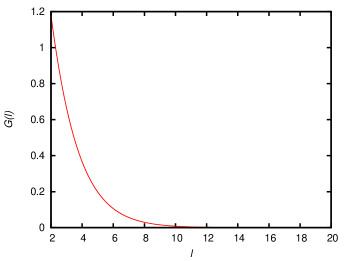
Figure 1: Plot of the function $G(l)$ [defined in (34)] in the range $2\leq l\leq 20$. The function $G(l)$, which encodes the correlation between the modes induced by the collapse, affects only the lowest multipoles

Clearly, by ignoring the transfer function, the traditional prediction of the angular power spectrum is a constant; on the other hand, in our approach, the mode correlation induced by the self-induced collapse, altered the standard prediction by adding the term $\lambda G(l)$. In Fig. (2a), we show a graphic of our predicted value for $l(l+1)C_{l}$ [normalized see Eq. (39)] with three different values of the $\lambda$ parameter and also a best-fit constant (799.25) to the data from Planck collaboration. In Fig. (2b) we show a plot for our predicted angular spectrum with the best-fit value $\lambda=-0.3039$ to Planck data. We see that our prediction is, in principle, able to improve the theoretical estimate to the observational data.

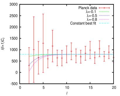
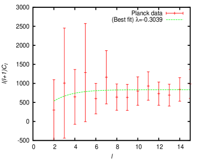
Figure 2: Fig. (2a) shows our predicted value for $l(l+1)C_{l}$ [Eq. (39) normalized] in the range $2\leq l\leq 20$ considering three values of $\lambda$ and the best-fit constant to the observational data from Planck collaboration. In Fig. (2b) we show our prediction for $l(l+1)C_{l}$ [Eq. (39) normalized] in the range $2\leq l\leq 15$ with the best-fit value $\lambda=-0.3039$ to Planck data.

As we can see, the effect is stronger for low $l$ and it decreases in a nearly exponential fashion for large $l$. For a more complete analysis, we should take into account the transfer functions $T(k)$ that are associated with the acoustic oscillations originated after the end of the inflationary era, this would lead to the full angular power spectrum. We want to emphasize that the result in Eq. (39) is different from the standard approach; first, it contains the function $g(z)$, which is a function of the time of collapse, and second, the correlation between different modes provided by the collapse is encoded in the function $G(l)$. Evidently, a more detailed analysis should be performed before reaching any conclusions, but this modest analysis shows the promising potential of our approach.

Expression (39) is the theoretical estimate to be compared with the observational data, and as should be clear from the discussion, the fact that we have to rely on most likely values, for what are in effect the mathematical equivalent of random walks, leads us to expect that there should be a general and rough agreement between our estimates and observations (assuming the theory is correct). However, we do not really expect a detailed and precise match simply due to the intrinsic randomness involved and characterized here in full in terms of the random numbers $X$. In the standard approach, similar considerations involving the randomness of the fluctuations and the uncertainties tied to stochasticity, mixed together with arguments involving the limited nature of the region of the universe one is observing, also lead to people in the community to expect small differences in predictions and observations. Nevertheless, in general, such discussions are based on heuristic arguments; therefore, are limited both in scope and precision. The essential difficulty is that, in the standard analysis, the precise stochastic elements are not identified and have no mathematical representation in the formalism. We believe that, the fact that in our approach, the stochastic elements are clearly identifiable (i.e. the $X_{\vec{k}}$), represents a great advantage. For instance, the formalism here provides us with an explicit expression for the quantity $a_{lm}$, such as in Eq. (27), and, thus, allowing us to study in great detail and in a transparent manner, the precise nature of higher order statistical estimates as we will do in the following.

III Characterizing the primordial CMB bispectrum

In this section, we will study the connection between the Newtonian potential at the end of inflation and the observational quantities obtained from the temperature anisotropies in the CMB; in particular, we will provide the connection between the parameters characterizing the collapse and the primordial bispectrum.

The usual path to look for non-trivial statistical features (e.g. possible non-Gaussianities) in the CMB is to study the bispectrum, which is considered to be directly related with the three-point function of the temperature anisotropies in harmonic space. The theoretical CMB angular bispectrum is defined as

$$B^{l_{1}l_{2}l_{3}}_{m_{1}m_{2}m_{3}}\equiv\overline{a_{1_{1}m_{1}}a_{1_{2}m_{2}}a_{1_{3}m_{3}}}.$$ (40)

The bar appearing in (40) denotes average over an ensemble of universes, but in practice such averaging is not viable and is usually “replaced,” in a sense, by averaging over orientations in our own universe; the relation between the two types of averages is not clear or direct (this fact has been discussed in great detail in Ref. susana2013 ). In the following, we will show how our approach helps to clarify certain issues that emerge when dealing with the statistical aspects of the spectrum and when comparing theoretical estimates and observations.

Given the definition of the CMB bispectrum and by using considerations involving the assumption of an (in average) rotational invariant sky, one finds in the literature komatsu2003 ; komatsu2009 another object called the “angle-averaged bispectrum” defined by

$$B_{l_{1}l_{2}l_{3}}\equiv\sum_{m_{i}}\left(\begin{array}[]{lcr}l_{1}&l_{2}&l_{3}\\ m_{1}&m_{2}&m_{3}\end{array}\right)B^{l_{1}l_{2}l_{3}}_{m_{1}m_{2}m_{3}}=\sum_{m_{i}}\left(\begin{array}[]{lcr}l_{1}&l_{2}&l_{3}\\ m_{1}&m_{2}&m_{3}\end{array}\right)\overline{a_{1_{1}m_{1}}a_{1_{2}m_{2}}a_{1_{3}m_{3}}}.$$ (41)

The object $\left(\begin{array}[]{lcr}l_{1}&l_{2}&l_{3}\\ m_{1}&m_{2}&m_{3}\end{array}\right)$ is called the Wigner 3-$j$ symbol (see Ref. Komatsu2001 for more details and properties for these functions); the bispectrum $B_{l_{1}l_{2}l_{3}}$ is non-vanishing for the values of $l,m$ satisfying the following conditions:

1. $m_{1}+m_{2}+m_{3}=0$.

2. $l_{1}+l_{2}+l_{3}$ is even.

3. $|l_{i}-l_{j}|\leq l_{k}\leq l_{i}+l_{j}$ for all permutations of indices.

Here it is important to mention that the 2nd. selection rule, comes not from the selection rules corresponding to the Wigner 3-j symbols, but from the additional assumption that the 3-point correlation function of the temperature anisotropies must be invariant under spatial rotations and translations Luo1994 ; Gangui1999 ; Gangui2000 . This is a crucial difference with our approach as we will see in the following. Also, the previous three selection rules are called “the triangle conditions” as $l_{1},l_{2},l_{3}$ must correspond to the sides of a triangle. As a matter of fact, in the standard approach, one intents to estimate $B_{l_{1}l_{2}l_{3}}$ from the observational data (e.g. see Sec. 3.1 of Ref. planckng ) by testing different configurations for such “triangles.”

Motivated by the fact that, when following our approach, we can obtain a direct relation between the coefficients $a_{lm}$ and the random variables characterizing the collapse [Eq. (27)] we will be focussing on the expression for the “observational” bispectrum:

$$\mathcal{B}^{\text{obs}}_{l_{1}l_{2}l_{3}}\equiv\sum_{m_{i}}\left(\begin{array}[]{lcr}l_{1}&l_{2}&l_{3}\\ m_{1}&m_{2}&m_{3}\end{array}\right)a_{1_{1}m_{1}}a_{1_{2}m_{2}}a_{1_{3}m_{3}}.$$ (42)

Note that this object also contains the Wigner 3-$j$ symbol, therefore, $l_{1},l_{2},l_{3}$ must satisfy the first and the third selection rule, meanwhile the 2nd. rule needs not to be satisfied, since the observed bispectrum is certainly not rotational nor translational invariant; the symmetry associated to the 2nd. selection rule applies to the average not to the observed bispectrum which is just one element (realization) of the “ensemble.” As a matter of fact, the more general rule, which encompass the 2nd. selection rule, for the Wigner 3-$j$ symbol is $l_{1}+l_{2}+l_{3}=$ integer (or even if $m_{1}=m_{2}=m_{3}=0$).

The difference between $B_{l_{1}l_{2}l_{3}}$ and $\mathcal{B}^{\text{obs}}_{l_{1}l_{2}l_{3}}$ is a subtle but important one. While in the definition of $B_{l_{1}l_{2}l_{3}}$ one should perform an average over an ensemble of universes [as is explicitly stated in the definition (41)], the object $\mathcal{B}^{\text{obs}}_{l_{1}l_{2}l_{3}}$ involves no averages over idealized ensembles whatsoever. The only average that is being performed in $\mathcal{B}^{\text{obs}}_{l_{1}l_{2}l_{3}}$, is an average over orientations (i.e. a sum over $m_{i}$ with a weight given by the Wigner 3-$j$ symbols).

In our approach, the prediction for $\mathcal{B}^{\text{obs}}_{l_{1}l_{2}l_{3}}$ is given explicitly by substituting (27) in (42) which yields

$$\mathcal{B}^{\text{obs}}_{l_{1}l_{2}l_{3}}=\sum_{m_{i}}\left(\begin{array}[]{lcr}l_{1}&l_{2}&l_{3}\\ m_{1}&m_{2}&m_{3}\end{array}\right)\frac{i^{l_{1}+l_{2}+l_{3}}}{L^{9/2}}\sum_{\vec{k}_{1},\vec{k}_{2},\vec{k}_{3}}g(z_{k_{1}})g(z_{k_{2}})g(z_{k_{3}})F_{l_{1}m_{1}}(\vec{k}_{1})F_{l_{2}m_{2}}(\vec{k}_{2})F_{l_{3}m_{3}}(\vec{k}_{3})X_{\vec{k}_{1}}X_{\vec{k}_{2}}X_{\vec{k}_{3}}.$$ (43)

As is clear from Eq. (43), the collapse bispectrum is in effect a sum of random complex numbers (i.e. a sum where each term is characterized by the product $X_{\vec{k}_{1}}X_{\vec{k}_{2}}X_{\vec{k}_{3}}$, which is itself, a complex random number), leading to what can be considered effectively as a two-dimensional (i.e. a complex plane) random walk, in complete analogy with what we found in dealing with our estimates of $a_{lm}$ in (27). Once more, one cannot give a perfect estimate for the final displacement resulting from the random walk. Nevertheless, one might give an estimate of its magnitude.

Similarly as $\mathcal{B}^{\text{obs}}_{l_{1}l_{2}l_{3}}$ is characterized by the sum of random variables we cannot give a specific value for its outcome. However, as we will see, and in complete analogy of our analysis of the quantities $a_{lm}$, by focusing on the most likely value of the magnitude $|\mathcal{B}^{\text{obs}}_{l_{1}l_{2}l_{3}}|^{2}$ we will obtain a reasonable prediction.

To recapitulate, the original situation corresponds to the homogeneous and isotropic vacuum state. When a sudden change of the initial state takes place due to the collapse (one for each mode), the mode becomes characterized by a fixed value of the corresponding random variables; the collection of all the values of such random variables associated to all the modes characterizes, therefore, our single and unique universe (so such numbers in consequence completely determine $|\mathcal{B}^{\text{obs}}_{l_{1}l_{2}l_{3}}|^{2}$); let us denote this set by

$$U=\{X_{\vec{k}},X_{\vec{k}^{\prime}},\ldots\}.$$ (44)

Nevertheless, given the stochastic nature of the collapse, we can consider that the universe could have corresponded to different set of values for the random variables characterizing the universe in a different manner $\tilde{U}=\{\tilde{X}_{\vec{k}},\tilde{X}_{\vec{k}^{\prime}},\ldots\}$. The collection of different sets $\{U,\tilde{U},\ldots\}$ thus describe an hypothetical ensemble of universes. We will denote the bispectrum associated to the hypothetical ensemble of universes as

$$\mathcal{B}_{l_{1}l_{2}l_{3}}(\xi)=\sum_{m_{i}}\left(\begin{array}[]{lcr}l_{1}&l_{2}&l_{3}\\ m_{1}&m_{2}&m_{3}\end{array}\right)\frac{i^{l_{1}+l_{2}+l_{3}}}{L^{9/2}}\sum_{\vec{k}_{1},\vec{k}_{2},\vec{k}_{3}}g(z_{k_{1}})g(z_{k_{2}})g(z_{k_{3}})F_{l_{1}m_{1}}(\vec{k}_{1})F_{l_{2}m_{2}}(\vec{k}_{2})F_{l_{3}m_{3}}(\vec{k}_{3})X_{\vec{k}_{1}}(\xi)X_{\vec{k}_{2}}(\xi)X_{\vec{k}_{3}}(\xi),$$ (45)

with the letter $\xi$ labeling the possible set of outcomes corresponding to the random variables that characterizes a particular Universe, thus, for example $\xi=\text{obs}$, corresponds to the bispectrum observed in our universe, this is Eq. (43), which we regard as typical member of this hypothetical ensemble.

Furthermore, we will (just as when dealing with $a_{lm}$), make the assumption that the most likely (M.L.) value of the magnitude $|\mathcal{B}_{l_{1}l_{2}l_{3}}(\xi)|^{2}$ in such ensemble is a good estimate of the corresponding one for our own universe, that is

$$|\mathcal{B}^{\text{obs}}_{l_{1}l_{2}l_{3}}|^{2}\simeq|\mathcal{B}_{l_{1}l_{2}l_{3}}(\xi)|^{2}_{\textrm{M.L.}}$$ (46)

Moreover, we can simplify the estimate by taking the ensemble average $\overline{|\mathcal{B}_{l_{1}l_{2}l_{3}}(\xi)|^{2}}$, i.e. the average over all possible outcomes of the bispectrum labeled by $\xi$ [Eq. (45)] and identify it with the most likely $|\mathcal{B}_{l_{1}l_{2}l_{3}}(\xi)|^{2}_{\textrm{M.L.}}$. It is needless to say that these two notions are not exactly the same for arbitrary kinds of ensembles; as a matter of fact, the relation between the two concepts depends on the probability distribution function (PDF) of the random variables. In principle, we do not know the exact PDF, as we have only access to a single realization–our own universe–, but as can bee seen from Eqs. (22), a very good approximation can be made by assuming that the PDF is highly Gaussian, this is, the parameter $\lambda$ which encodes the correlation between the modes caused by the collapse, is small enough that a Gaussian PDF for the random variables is justified. Therefore, we can approximate

$$|\mathcal{B}_{l_{1}l_{2}l_{3}}(\xi)|^{2}_{\textrm{M. L.}}\simeq\overline{|\mathcal{B}_{l_{1}l_{2}l_{3}}(\xi)|^{2}},$$ (47)

which implies that

$$|\mathcal{B}^{\text{obs}}_{l_{1}l_{2}l_{3}}|^{2}\simeq|\mathcal{B}_{l_{1}l_{2}l_{3}}(\xi)|^{2}_{\textrm{M. L.}}\simeq\overline{|\mathcal{B}_{l_{1}l_{2}l_{3}}(\xi)|^{2}}.$$ (48)

In the reminder of this section, we will focus on computing $\overline{|\mathcal{B}_{l_{1}l_{2}l_{3}}(\xi)|^{2}}$ and will omit the label $\xi$ with the understanding that it represents the ensemble over possible outcomes of $\xi$. Therefore, the ensemble average is

$$\overline{|\mathcal{B}_{l_{1}l_{2}l_{3}}|^{2}}=\sum_{m_{1},\ldots,m_{6}}\left(\begin{array}[]{lcr}l_{1}&l_{2}&l_{3}\\ m_{1}&m_{2}&m_{3}\end{array}\right)\left(\begin{array}[]{lcr}l_{1}&l_{2}&l_{3}\\ m_{4}&m_{5}&m_{6}\end{array}\right)\overline{a_{l_{1}m_{1}}a_{l_{2}m_{2}}a_{l_{3}m_{3}}a_{l_{1}m_{4}}^{\star}a_{l_{2}m_{5}}^{\star}a_{l_{3}m_{6}}^{\star}}.$$ (49)

Let us focus on the quantity $\overline{a_{l_{1}m_{1}}a_{l_{2}m_{2}}a_{l_{3}m_{3}}a_{l_{1}m_{4}}^{\star}a_{l_{2}m_{5}}^{\star}a_{l_{3}m_{6}}^{\star}}$, thus using Eq. (27) gives

$$\overline{a_{l_{1}m_{1}}a_{l_{2}m_{2}}a_{l_{3}m_{3}}a_{l_{1}m_{4}}^{\star}a_{l_{2}m_{5}}^{\star}a_{l_{3}m_{6}}^{\star}} = \frac{1}{L^{6}}\sum_{\vec{k}_{1},\ldots,\vec{k}_{6}}g(z_{k_{1}})g(z_{k_{2}})g(z_{k_{3}})g(z_{k_{4}})g(z_{k_{5}})g(z_{k_{6}})$$ (50)

$$\times F_{l_{1}m_{1}}(\vec{k}_{1})F_{l_{2}m_{2}}(\vec{k}_{2})F_{l_{3}m_{3}}(\vec{k}_{3})F_{l_{1}m_{4}}^{*}(\vec{k}_{4})F_{l_{2}m_{5}}^{*}(\vec{k}_{5})F_{l_{3}m_{6}}^{*}(\vec{k}_{6})$$

$$\times \overline{X_{\vec{k}_{1}}X_{\vec{k}_{2}}X_{\vec{k}_{3}}X_{\vec{k}_{4}}^{*}X_{\vec{k}_{5}}^{*}X_{\vec{k}_{6}}^{*}}.$$

As we are assuming that the $X_{\vec{k}}$ follow a highly Gaussian PDF, then we can approximate the 6th momentum distribution by:

$$\overline{X_{\vec{k}_{1}}X_{\vec{k}_{2}}X_{\vec{k}_{3}}X^{\star}_{\vec{k}_{4}}X^{\star}_{\vec{k}_{5}}X^{\star}_{\vec{k}_{6}}} =$$

$$\overline{X_{\vec{k}_{1}}X_{\vec{k}_{2}}}\cdot\overline{X_{\vec{k}_{3}}X_{\vec{k}_{4}}^{\star}}\cdot\overline{X_{\vec{k}_{5}}^{\star}X_{\vec{k}_{6}}^{\star}} + \overline{X_{\vec{k}_{1}}X_{\vec{k}_{2}}}\cdot\overline{X_{\vec{k}_{3}}X_{\vec{k}_{5}}^{\star}}\cdot\overline{X_{\vec{k}_{4}}^{\star}X_{\vec{k}_{6}}^{\star}}+\overline{X_{\vec{k}_{1}}X_{\vec{k}_{2}}}\cdot\overline{X_{\vec{k}_{3}}X_{\vec{k}_{6}}^{\star}}\cdot\overline{X_{\vec{k}_{4}}^{\star}X_{\vec{k}_{5}}^{\star}}$$

$$+\overline{X_{\vec{k}_{1}}X_{\vec{k}_{3}}}\cdot\overline{X_{\vec{k}_{2}}X_{\vec{k}_{4}}^{\star}}\cdot\overline{X_{\vec{k}_{5}}^{\star}X_{\vec{k}_{6}}^{\star}} + \overline{X_{\vec{k}_{1}}X_{\vec{k}_{3}}}\cdot\overline{X_{\vec{k}_{2}}X_{\vec{k}_{5}}^{\star}}\cdot\overline{X_{\vec{k}_{4}}^{\star}X_{\vec{k}_{6}}^{\star}}+\overline{X_{\vec{k}_{1}}X_{\vec{k}_{3}}}\cdot\overline{X_{\vec{k}_{2}}X_{\vec{k}_{6}}^{\star}}\cdot\overline{X_{\vec{k}_{4}}^{\star}X_{\vec{k}_{5}}^{\star}}$$

$$+\overline{X_{\vec{k}_{1}}X_{\vec{k}_{4}}^{\star}}\cdot\overline{X_{\vec{k}_{2}}X_{\vec{k}_{3}}}\cdot\overline{X_{\vec{k}_{5}}^{\star}X_{\vec{k}_{6}}^{\star}} + \overline{X_{\vec{k}_{1}}X_{\vec{k}_{4}}^{\star}}\cdot\overline{X_{\vec{k}_{2}}X_{\vec{k}_{5}}^{\star}}\cdot\overline{X_{\vec{k}_{3}}X_{\vec{k}_{6}}^{\star}}+\overline{X_{\vec{k}_{1}}X_{\vec{k}_{4}}^{\star}}\cdot\overline{X_{\vec{k}_{2}}X_{\vec{k}_{6}}^{\star}}\cdot\overline{X_{\vec{k}_{3}}X_{\vec{k}_{5}}^{\star}}$$

$$+\overline{X_{\vec{k}_{1}}X_{\vec{k}_{5}}^{\star}}\cdot\overline{X_{\vec{k}_{2}}X_{\vec{k}_{3}}}\cdot\overline{X_{\vec{k}_{4}}^{\star}X_{\vec{k}_{6}}^{\star}} + \overline{X_{\vec{k}_{1}}X_{\vec{k}_{5}}^{\star}}\cdot\overline{X_{\vec{k}_{2}}X_{\vec{k}_{4}}^{\star}}\cdot\overline{X_{\vec{k}_{3}}X_{\vec{k}_{6}}^{\star}}+\overline{X_{\vec{k}_{1}}X_{\vec{k}_{5}}^{\star}}\cdot\overline{X_{\vec{k}_{2}}X_{\vec{k}_{6}}^{\star}}\cdot\overline{X_{\vec{k}_{3}}X_{\vec{k}_{4}}^{\star}}$$

$$+\overline{X_{\vec{k}_{1}}X_{\vec{k}_{6}}^{\star}}\cdot\overline{X_{\vec{k}_{2}}X_{\vec{k}_{3}}}\cdot\overline{X_{\vec{k}_{4}}^{\star}X_{\vec{k}_{5}}^{\star}} + \overline{X_{\vec{k}_{1}}X_{\vec{k}_{6}}^{\star}}\cdot\overline{X_{\vec{k}_{2}}X_{\vec{k}_{4}}^{\star}}\cdot\overline{X_{\vec{k}_{3}}X_{\vec{k}_{5}}^{\star}}+\overline{X_{\vec{k}_{1}}X_{\vec{k}_{6}}^{\star}}\cdot\overline{X_{\vec{k}_{2}}X_{\vec{k}_{5}}^{\star}}\cdot\overline{X_{\vec{k}_{3}}X_{\vec{k}_{4}}^{\star}}.$$

Therefore, substituting Eq. (III) into Eq. (50) yields

$$\overline{a_{l_{1}m_{1}}a_{l_{2}m_{2}}a_{l_{3}m_{3}}a_{l_{1}m_{4}}^{\star}a_{l_{2}m_{5}}^{\star}a_{l_{3}m_{6}}^{\star}}=$$ (52)

$$\frac{1}{L^{6}}\sum_{\vec{k}_{1},\ldots,\vec{k}_{6}}g(z_{k_{1}})g(z_{k_{2}})g(z_{k_{3}})g(z_{k_{4}})g(z_{k_{5}})g(z_{k_{6}})F_{l_{1}m_{1}}(\vec{k}_{1})F_{l_{2}m_{2}}(\vec{k}_{2})F_{l_{3}m_{3}}(\vec{k}_{3})F_{l_{1}m_{4}}^{*}(\vec{k}_{4})F_{l_{2}m_{5}}^{*}(\vec{k}_{5})F_{l_{3}m_{6}}^{*}(\vec{k}_{6})$$

$$\times \left(\overline{X_{\vec{k}_{1}}X_{\vec{k}_{2}}}\cdot\overline{X_{\vec{k}_{3}}X_{\vec{k}_{4}}^{*}}\cdot\overline{X_{\vec{k}_{5}}^{*}X_{\vec{k}_{6}}^{*}}+14\text{ permutations}\right)$$

$$= \frac{1}{L^{6}}\left(\sum_{\vec{k}_{1},\vec{k}_{2}}g(z_{k_{1}})g(z_{k_{2}})F_{l_{1}m_{1}}(\vec{k}_{1})F_{l_{2}m_{2}}(\vec{k}_{2})\overline{X_{\vec{k}_{1}}X_{\vec{k}_{2}}}\right)\left(\sum_{\vec{k}_{3},\vec{k}_{4}}g(z_{k_{3}})g(z_{k_{4}})F_{l_{3}m_{3}}(\vec{k}_{3})F_{l_{1}m_{4}}^{*}(\vec{k}_{4})\overline{X_{\vec{k}_{3}}X_{\vec{k}_{4}}^{*}}\right)$$

$$\times \left(\sum_{\vec{k}_{5},\vec{k}_{6}}g(z_{k_{5}})g(z_{k_{6}})F_{l_{1}m_{1}}^{*}(\vec{k}_{5})F_{l_{2}m_{2}}^{*}(\vec{k}_{6})\overline{X_{\vec{k}_{5}}^{*}X_{\vec{k}_{6}}^{*}}\right)+14\textrm{ permutations}$$

$$= \overline{a_{l_{1}m_{1}}a_{l_{2}m_{2}}}\cdot\overline{a_{l_{3}m_{3}}a_{l_{1}m_{4}}^{*}}\cdot\overline{a_{l_{2}m_{5}}^{*}a_{l_{3}m_{6}}^{*}}+14\textrm{ permutations,}$$

where the last step uses Eq. (30). This is an expected result from the beginning because the $a_{lm}$ and the $X_{\vec{k}}$ are linearly related, hence, the $a_{lm}$ must have the same statistics as the $X_{\vec{k}}$, which we have assumed to be highly Gaussian. Thus, all higher order correlators must either be zero (odd) or products of the two-point correlator (even). Of the 15 permutations, there are 6 of the form $\overline{aa^{*}}\cdot\overline{aa^{*}}\cdot\overline{aa^{*}}$ and 9 of the form $\overline{aa}\cdot\overline{aa^{*}}\cdot\overline{a^{*}a^{*}}$. Let us consider the second case first and its relation with $\overline{|\mathcal{B}_{l_{1}l_{2}l_{3}}|^{2}}$; e.g. let us analyze the term

$$\sum_{m_{1},\ldots,m_{6}} \left(\begin{array}[]{lcr}l_{1}&l_{2}&l_{3}\\ m_{1}&m_{2}&m_{3}\end{array}\right)\left(\begin{array}[]{lcr}l_{1}&l_{2}&l_{3}\\ m_{4}&m_{5}&m_{6}\end{array}\right)\overline{a_{l_{1}m_{1}}a_{l_{2}m_{2}}}\cdot\overline{a_{l_{3}m_{3}}a_{l_{1}m_{4}}^{*}}\cdot\overline{a_{l_{2}m_{5}}^{*}a_{l_{3}m_{6}}^{*}}$$ (57)

$$= \sum_{m_{1},\ldots,m_{6}}\left(\begin{array}[]{lcr}l_{1}&l_{2}&l_{3}\\ m_{1}&m_{2}&m_{3}\end{array}\right)\left(\begin{array}[]{lcr}l_{1}&l_{2}&l_{3}\\ m_{4}&m_{5}&m_{6}\end{array}\right)(-1)^{m_{1}}D_{l_{1}}\delta_{l_{1},l_{2}}\delta_{m_{1},-m_{2}}D_{l_{3}}\delta_{l_{3},l_{1}}\delta_{m_{3},m_{4}}(-1)^{m_{5}}D_{l_{2}}\delta_{l_{2},l_{3}}\delta_{m_{5},-m_{6}}$$ (62)

$$= D_{l_{1}}D_{l_{2}}D_{l_{3}}\delta_{l_{1},l_{2}}\delta_{l_{2},l_{3}}\sum_{m_{1},m_{3},m_{5}}\left(\begin{array}[]{lcr}l_{1}&l_{1}&l_{3}\\ m_{1}&-m_{1}&m_{3}\end{array}\right)\left(\begin{array}[]{lcr}l_{3}&l_{1}&l_{1}\\ m_{3}&m_{5}&-m_{5}\end{array}\right)(-1)^{m_{1}+m_{5}}$$ (67)

$$= D_{l_{1}}D_{l_{2}}D_{l_{3}}\delta_{l_{1},l_{2}}\delta_{l_{2},l_{3}}\left(\sum_{m_{1}}\left(\begin{array}[]{lcr}l_{1}&l_{1}&l_{3}\\ m_{1}&-m_{1}&0\end{array}\right)(-1)^{m_{1}}\right)\left(\sum_{m_{5}}\left(\begin{array}[]{lcr}l_{1}&l_{1}&l_{3}\\ m_{5}&-m_{5}&0\end{array}\right)(-1)^{m_{5}}\right)$$ (72)

$$= D_{l_{1}}D_{l_{2}}D_{l_{3}}\delta_{l_{1},l_{2}}\delta_{l_{2},l_{3}}(2l_{1}+1)\delta_{l_{3},0},$$ (73)

where in the second line we used the relations given in Eq. (32); in the fourth line we used the selection rule for Wigner 3-$j$ symbols, and in the last line we used an identity for the sum of the Wigner 3-$j$ symbols. Consequently, since this term is proportional to the monopole ($l=0$), which is unobservable, then it vanishes. The same occurs in all 9 terms. Henceforth, all that remains are the 6 terms that we will consider now. Once again, focusing a typical term, e.g.

$$\sum_{m_{1},\ldots,m_{6}} \left(\begin{array}[]{lcr}l_{1}&l_{2}&l_{3}\\ m_{1}&m_{2}&m_{3}\end{array}\right)\left(\begin{array}[]{lcr}l_{1}&l_{2}&l_{3}\\ m_{4}&m_{5}&m_{6}\end{array}\right)\overline{a_{l_{1}m_{1}}a_{l_{1}m_{4}}^{*}}\cdot\overline{a_{l_{2}m_{2}}a_{l_{2}m_{5}}^{*}}\cdot\overline{a_{l_{3}m_{3}}a_{l_{3}m_{6}}^{*}}$$ (78)

$$= \sum_{m_{1},\ldots,m_{6}}\left(\begin{array}[]{lcr}l_{1}&l_{2}&l_{3}\\ m_{1}&m_{2}&m_{3}\end{array}\right)\left(\begin{array}[]{lcr}l_{1}&l_{2}&l_{3}\\ m_{4}&m_{5}&m_{6}\end{array}\right)D_{l_{1}}\delta_{m_{1},m_{4}}D_{l_{2}}\delta_{m_{2},m_{5}}D_{l_{3}}\delta_{m_{3},m_{6}}$$ (83)

$$= D_{l_{1}}D_{l_{2}}D_{l_{3}}\left[\sum_{m_{1},m_{2},m_{3}}\left(\begin{array}[]{lcr}l_{1}&l_{2}&l_{3}\\ m_{1}&m_{2}&m_{3}\end{array}\right)\right]^{2}$$ (86)

$$= D_{l_{1}}D_{l_{2}}D_{l_{3}},$$ (87)

where in the second line we used Eq. (32) and in the last line we used an identity of the Wigner 3-$j$ symbols. The remaining 5 terms are computed in a similar way. The final result is thus

$$\overline{|\mathcal{B}_{l_{1}l_{2}l_{3}}|^{2}}=D_{l_{1}}D_{l_{2}}D_{l_{3}}\left[1+\delta_{l_{1},l_{2}}(-1)^{l_{3}+2l_{1}}+\delta_{l_{2},l_{3}}(-1)^{l_{1}+2l_{2}}+\delta_{l_{3},l_{1}}(-1)^{l_{2}+2l_{3}}+2\delta_{l_{1},l_{2}}\delta_{l_{2},l_{3}}\right],$$ (88)

with $l=1,2,\ldots$. Consequently, the most likely value for the magnitude of the collapse bispectrum is $|\mathcal{B}_{l_{1}l_{2}l_{3}}|_{\textrm{M.L.}}=\left(\overline{|\mathcal{B}_{l_{1}l_{2}l_{3}}|^{2}}\right)^{1/2}$, i.e.

$$|\mathcal{B}_{l_{1}l_{2}l_{3}}|_{\textrm{M.L.}} = \frac{1}{\pi^{3/2}}\left(\frac{H}{10M_{P}\epsilon^{1/2}}\right)^{3}\left|\cos z-\frac{\sin z}{z}\right|^{3}\left\{\frac{[1+\lambda G(l_{1})][1+\lambda G(l_{2})][1+\lambda G(l_{3})]}{l_{1}(l_{1}+1)l_{2}(l_{2}+1)l_{3}(l_{3}+1)}\right\}^{1/2}$$ (89)

$$\times \left[1+\delta_{l_{1},l_{2}}(-1)^{l_{3}+2l_{1}}+\delta_{l_{2},l_{3}}(-1)^{l_{1}+2l_{2}}+\delta_{l_{3},l_{1}}(-1)^{l_{2}+2l_{3}}+2\delta_{l_{1},l_{2}}\delta_{l_{2},l_{3}}\right]^{1/2},$$

where we used the definition of $D_{l}$ and $g(z)$ given in Eqs. (33) and (29) respectively.

Equation (89) is the main result of this section. Given the definition of Eq. (42), $l_{1},l_{2},l_{3}$ must correspond to the sides of a triangle, otherwise $|\mathcal{B}_{l_{1}l_{2}l_{3}}|_{\textrm{M.L.}}=0$ just as in standard treatments.

However we must emphasize that $|\mathcal{B}_{l_{1}l_{2}l_{3}}|$ is not exactly the same as the magnitude of the traditional theoretical angle-averaged-bispectrum $|B_{l_{1}l_{2}l_{3}}|$, as the latter would correspond to the ensemble average as defined in Eq. (41). In fact, in the conventional approach, one would relate an average over an ensemble of universes to a certain quantum three-point function, which would of course vanish in the absence of “non-Gaussianities.” In the standard approach argument then proceeds, by identifying the average over the ensemble of possible universes with the angle-averaged-bispectrum $B_{l_{1}l_{2}l_{3}}$, which is just a orientation average in the only universe we have access to. Thus the theoretical quantity is connected with suitable averages over $m$’s of the quantity $a_{l_{1}m_{1}}a_{l_{2}m_{2}}a_{l_{2}m_{3}}$ measured in our own (single) universe.

Our point is, thus, connected with the fact that these series of identifications do not have a fully transparent and clear justification (as discussed in detail in Ref. susana2013 ); and this, in our view, makes it very difficult to deal, in a clear way, with existing and potential delicate issues. One example of such difficulty arises when wanting to study issues concerning say large deviations from isotropy in the observed CMB. On the other hand, within the collapse model, we find a prediction for the most likely value of $|\mathcal{B}_{l_{1}l_{2}l_{3}}|_{\textrm{M.L.}}$ which can be related directly with the actual observational quantity:

$$|B_{l_{1}l_{2}l_{3}}|_{\textrm{ Actual obs}}\equiv\left|\sum_{m_{i}}\left(\begin{array}[]{lcr}l_{1}&l_{2}&l_{3}\\ m_{1}&m_{2}&m_{3}\end{array}\right)(a_{l_{1}m_{1}}a_{l_{2}m_{2}}a_{l_{2}m_{3}})_{\textrm{ Actual obs}}\right|,$$ (90)

in a much more direct and transparent manner. Note, however, that we make a distinction between the theory’s prediction for the most likely value of the observational quantity $|\mathcal{B}_{l_{1}l_{2}l_{3}}|_{\textrm{M.L.}}$ and the actually observed quantity itself $|B_{l_{1}l_{2}l_{3}}|_{\textrm{Actual obs}}$. This is exactly analogous to the distinction beteen a theory prediction of the most likely value of the total displacement in a random walk, and the actual displacement observed in a single realization of said walk.

At this point it is also convenient to clarify certain aspects within our approach. Some readers may claim that our expression for the observed bispectrum is equivalent to the cosmic variance of the bispectrum, within the standard approach, in the “weak non-Gaussian” limit. In other words, the fact that we used the approximation in Eq. (III), corresponding to a highly Gaussian PDF for the random parameters of the collapse, could lead some people to state that what we are computing is actually the variance of the traditional bispectrum, Eq. (41), when $B_{l_{1},l_{2},l_{3}}=0$. This is partially correct and a few remarks are in order.

If $\lambda=0$, which means that the PDF of the random collapse parameters is exactly Gaussian, and if $l_{1}+l_{2}+l_{3}$ is even, then our expression for $|\mathcal{B}_{l_{1}l_{2}l_{3}}|_{\textrm{M.L.}}$ coincides exactly with the traditional estimation of the variance of the bispectrum in the Gaussian limit Luo1994 ; Gangui1999 ; Gangui2000 , i.e. $\textrm{Var}[B_{l_{1}l_{2}l_{3}}]\propto C_{l_{1}}C_{l_{2}}C_{l_{3}}$, with $C_{l}$ the angular power spectrum which is of the form $C_{l}\propto 1/l(l+1)$ in the range $l\leq 20$. On the other hand, if $\lambda\neq 0$, which physically means that the collapse of the wave function correlates different modes, then our expression (89), contains a function $G(l)$ that is absent in the traditional approach. Furthermore, as we mentioned previously, in our approach there is in principle no restriction on $l_{1}+l_{2}+l_{3}$ (which in the standard approach must be even a and represents an extra requirement for the nonvanishing of the bispectrum) as we are not assuming that the ensemble average of the bispectrum coincides with the observed one, this is, we do not basin our analysis in anything analogous to the standard claim that the 3-point correlation function of the temperature anisotropies must be rotational and translational invariant. This aspect of our analysis, represent a difference in the predictions that can be confronted with observations. In the next section, we will extend this and other discussions about the relation between the statistical aspects of the traditional bispectrum and the collapse bispectrum.

IV Main differences between the standard and the collapse approach regarding the primordial bispectrum

IV.1 The standard approach to the CMB bispectrum

We begin this section by giving a rather brief review of the conventional approach to the study of the primordial bispectrum, its amplitude and the usual arguments given to relate it with possible non-Gaussian features in the perturbations; extended reviews can be found in Refs. bartolo2004 ; komatsu2003 ; Yadav ; Liguori ; Komatsu2001 .

According to the standard approach, if $\Psi(\vec{x},\eta)$ is taken to be characterized by a Gaussian distribution all its statistical properties are codified in the two-point correlation function. Otherwise, one needs to consider higher order correlation functions, e.g. the three-point correlation function $\overline{\Psi(\vec{x},\eta)\Psi(\vec{y},\eta)\Psi(\vec{z},\eta)}$. The Fourier transform is commonly referred as the bispectrum, defined by

$$\overline{\Psi_{\vec{k}_{1}}\Psi_{\vec{k}_{2}}\Psi_{\vec{k}_{2}}}\equiv(2\pi)^{3}\delta(\vec{k}_{1}+\vec{k}_{2}+\vec{k}_{3})B_{\Psi}(k_{1},k_{2},k_{3}).$$ (91)

The Dirac delta appearing in Eq. (91) is said to indicate that the ensemble average $\overline{\Psi(\vec{x},\eta)\Psi(\vec{y},\eta)\Psi(\vec{z},\eta)}$ is invariant under spatial translations; in addition, the dependence only on the magnitudes $k$, appearing in the function $B_{\Psi}(k_{1},k_{2},k_{3})$, is tied to the rotational invariance of such ensemble. The Dirac delta constrains the three modes involved; this is, the modes must satisfy $\vec{k}_{1}+\vec{k}_{2}+\vec{k}_{3}=0$, which is known as the triangle condition. Thus, according to the direct relation of the Newtonian potential with the source of the observed anisotropies, the assumption about the rotational and translational invariance of the ensemble and its impact on $\overline{\Psi(\vec{x},\eta)\Psi(\vec{y},\eta)\Psi(\vec{z},\eta)}$ should be reflected in the invariance of the ensemble average of the temperature fluctuations $\overline{\frac{\delta T}{T_{0}}(\theta_{1},\varphi_{1})\frac{\delta T}{T_{0}}{(\theta_{2},\varphi_{2})}\frac{\delta T}{T_{0}}(\theta_{3},\varphi_{3})}$. However, we should once again emphasize that strictly speaking the discussion above and, thus, the average indicated by the overline in the latter expressions, refers to an average over an ensemble of universes and not averages over orientations in one universe.

One of the first (and most popular ways) to parameterize the traditional non-Gaussianity phenomenologically is via the introduction of a non-linear correction to the linear Gaussian curvature perturbation salopek1990 ; salopek1991 ,

$$\Psi(\vec{x},\eta)=\Psi_{g}(\vec{x},\eta)+f_{\textrm{NL}}^{\textrm{loc}}[\Psi_{g}^{2}(\vec{x},\eta)-\overline{\Psi_{g}^{2}(\vec{x},\eta)}],$$ (92)

where $\Psi_{g}(\vec{x},\eta)$ denotes a linear Gaussian part of the perturbation and $\overline{\Psi_{g}^{2}(\vec{x},\eta)}$ is the variance of the of the Gaussian part. The parameter $f_{\textrm{NL}}^{\textrm{loc}}$ is called the “local non-linear coupling parameter” and determines the “strength” of the primordial non-Gaussianity. This parametrization of non-Gaussianity is local in real space and therefore is called “local non-Gaussianity.” Using Eqs. (91) and (92), the bispectrum of local non-Gaussianity may be derived:

$$B_{\Psi}(\vec{k}_{1},\vec{k}_{2},\vec{k}_{3}) = 2f_{\textrm{NL}}^{\textrm{loc}}[P_{\Psi}(\vec{k}_{1})P_{\Psi}(\vec{k}_{2})+P_{\Psi}(\vec{k}_{2})P_{\Psi}(\vec{k}_{3})+P_{\Psi}(\vec{k}_{3})P_{\Psi}(\vec{k}_{1})]$$ (93)

$$= 2f_{\textrm{NL}}^{\textrm{loc}}\frac{A^{2}_{\Psi}}{(k_{1}k_{2}k_{3})^{2}}\left(\frac{k_{1}^{2}}{k_{2}k_{3}}+\frac{k_{2}^{2}}{k_{1}k_{3}}+\frac{k_{3}^{2}}{k_{1}k_{2}}\right),$$

with $P_{\Psi}(\vec{k})$ the power spectrum of the Newtonian potential defined as $\overline{\Psi(\vec{k})\Psi(\vec{k}^{\prime})}\equiv(2\pi)^{3}\delta(\vec{k}+\vec{k}^{\prime})P_{\Psi}(k)$ and it is assumed to be of the form $P_{\Psi}(\vec{k})=A_{\Psi}k^{-3}$, where $A_{\Psi}$ denotes the amplitude of the power spectrum.

Expressing the coefficients $a_{lm}$ in terms of $\Psi_{\vec{k}}$ as in Eq. (26) and using Eq. (91), one can proceed to compute the CMB bispectrum, defined in Eq. (40), this is

$$B^{l_{1}l_{2}l_{3}}_{m_{1}m_{2}m_{3}} = \overline{a_{l_{1}m_{1}}a_{l_{2}m_{2}}a_{l_{3}m_{3}}}$$

$$= \bigg{(}\frac{4\pi}{3}\bigg{)}^{3}i^{l_{1}+l_{2}+l_{3}}\int\frac{d^{3}k_{1}}{(2\pi)^{3}}\frac{d^{3}k_{2}}{(2\pi)^{3}}\frac{d^{3}k_{3}}{(2\pi)^{3}}j_{l_{1}}(k_{1}R_{D})j_{l_{2}}(k_{2}R_{D})j_{l_{3}}(k_{3}R_{D})$$

$$\times T(k_{1})T(k_{2})T(k_{3})\overline{\Psi_{\vec{k}_{1}}\Psi_{\vec{k}_{2}}\Psi_{\vec{k}_{3}}}Y_{l_{1}m_{1}}(\hat{k_{1}})Y_{l_{2}m_{2}}(\hat{k_{2}})Y_{l_{3}m_{3}}(\hat{k_{3}})$$

$$= \bigg{(}\frac{2}{\pi}\bigg{)}^{3}\int dk_{1}dk_{2}dk_{3}\textrm{ }(k_{1}k_{2}k_{3})^{2}T(k_{1})T(k_{2})T(k_{3})j_{l_{1}}(k_{1}R_{D})j_{l_{2}}(k_{2}R_{D})j_{l_{3}}(k_{3}R_{D})$$

$$\times B_{\Psi}(k_{1},k_{2},k_{3})\int_{0}^{\infty}dx\textrm{ }x^{2}j_{l_{1}}(k_{1}x)j_{l_{2}}(k_{2}x)j_{l_{3}}(k_{3}x)\int d\Omega_{\hat{x}}Y_{l_{1}m_{1}}(\hat{x})Y_{l_{2}m_{2}}(\hat{x})Y_{l_{3}m_{3}}(\hat{x}),$$

where in the last line, one performs the integral over the directions of the three vectors $k_{i}$ and use the exponential integral form for the delta function that appears in the bispectrum definition (91). The integral over the angular part of $\vec{x}$, in the last line, is known as the Gaunt integral, i.e.,

$$\mathcal{G}_{l_{1}l_{2}l_{3}}^{m_{1}m_{2}m_{3}} \equiv \int d\Omega_{\hat{x}}Y_{l_{1}m_{1}}(\hat{x})Y_{l_{2}m_{2}}(\hat{x})Y_{l_{3}m_{3}}(\hat{x})$$ (99)

$$= \sqrt{\frac{(2l_{1}+1)(2l_{2}+1)(2l_{3}+1)}{4\pi}}\left(\begin{array}[]{lcr}l_{1}&l_{2}&l_{3}\\ 0&0&0\end{array}\right)\left(\begin{array}[]{lcr}l_{1}&l_{2}&l_{3}\\ m_{1}&m_{2}&m_{3}\end{array}\right).$$

The fact that the bispectrum $B_{m_{1}m_{2}m_{3}}^{l_{1}l_{2}l_{3}}$ turns out to be proportional of the Gaunt integral, $\mathcal{G}_{l_{1}l_{2}l_{3}}^{m_{1}m_{2}m_{3}}$, implies that the values of $l,m$, corresponding to the non-vanishing components of the bispectrum, must satisfy “the triangle conditions” and also reflect the fact that in the definition of the bispectrum there is a Dirac delta [Eq. (91)] which guarantees the rotational invariance for the ensemble average $\overline{\Psi_{\vec{k}_{1}}\Psi_{\vec{k}_{2}}\Psi_{\vec{k}_{3}}}$.

One can find a close form for the bispectrum by choosing to work in the Sach-Wolfe approximation, where the transfer function $T(k)=1$; thus, substituting Eq. (93) into Eq. (IV.1) and evaluating the remaining integrals one obtains (See Ref. fergusson2009 ):

$$B^{l_{1}l_{2}l_{3}}_{m_{1}m_{2}m_{3}} = \mathcal{G}_{l_{1}l_{2}l_{3}}^{m_{1}m_{2}m_{3}}f_{\textrm{NL}}^{\textrm{loc}}\left(\frac{2A_{\Psi}^{2}}{27\pi^{2}}\right)\bigg{(}\frac{1}{l_{1}(l_{1}+1)l_{2}(l_{2}+1)}+\frac{1}{l_{2}(l_{2}+1)l_{3}(l_{3}+1)}$$ (100)

$$+ \frac{1}{l_{1}(l_{1}+1)l_{3}(l_{3}+1)}\bigg{)}.$$

Finally, using the definition of the angle-averaged-bispectrum [Eq. (41)], one has

$$B_{l_{1}l_{2}l_{3}} = \sqrt{\frac{(2l_{1}+1)(2l_{2}+1)(2l_{3}+1)}{4\pi}}\left(\begin{array}[]{lcr}l_{1}&l_{2}&l_{3}\\ 0&0&0\end{array}\right)f_{\textrm{NL}}^{\textrm{loc}}\left(\frac{2A_{\Psi}^{2}}{27\pi^{2}}\right)$$ (103)

$$\times \left(\frac{1}{l_{1}(l_{1}+1)l_{2}(l_{2}+1)}+\frac{1}{l_{2}(l_{2}+1)l_{3}(l_{3}+1)}+\frac{1}{l_{1}(l_{1}+1)l_{3}(l_{3}+1)}\right).$$ (104)

When working within the standard scenario for slow-roll inflation (and thus a “nearly” scale-invariant spectrum), Maldacena found that the estimate for the amplitude of non-Gaussianities of the local form, is $f_{\textrm{NL}}^{\textrm{loc}}\simeq\epsilon$ maldacena2002 (this is assumed to be in the limit when $k_{1}\ll k_{2}\simeq k_{3}$, i.e. in the so-called “squeezed” configuration). As seen from the previous discussion, in the conventional approach, the amplitude of the primordial bispectrum and the non-Gaussian statistics for the curvature perturbation are intrinsically related.

IV.2 Comparing the magnitude of the collapse and the traditional bispectrum

The magnitude of $|B_{l_{1}l_{2}l_{3}}|$ is obtained from Eq. (103)

$$|B_{l_{1}l_{2}l_{3}}| = \sqrt{\frac{(2l_{1}+1)(2l_{2}+1)(2l_{3}+1)}{4\pi}}\left|\left(\begin{array}[]{lcr}l_{1}&l_{2}&l_{3}\\ 0&0&0\end{array}\right)\right||f_{\textrm{NL}}^{\textrm{loc}}|\left(\frac{2H^{4}}{27\pi^{2}M_{P}^{4}\epsilon^{2}}\right)$$ (107)

$$\times \left(\frac{1}{l_{1}(l_{1}+1)l_{2}(l_{2}+1)}+\frac{1}{l_{2}(l_{2}+1)l_{3}(l_{3}+1)}+\frac{1}{l_{1}(l_{1}+1)l_{3}(l_{3}+1)}\right);$$ (108)

where we have used the estimate for the amplitude of the power spectrum for a single scalar field in the slow-roll scenario, given by $A_{\Psi}\simeq H^{2}/(M_{P}^{2}\epsilon)$.

On the other hand, the magnitude of the collapse biscpectrum is given by Eq. (89), which we will write again

$$|\mathcal{B}_{l_{1}l_{2}l_{3}}|_{\textrm{M.L.}} = \frac{1}{\pi^{3/2}}\left(\frac{H}{10M_{P}\epsilon^{1/2}}\right)^{3}\left|\cos z-\frac{\sin z}{z}\right|^{3}\left\{\frac{[1+\lambda G(l_{1})][1+\lambda G(l_{2})][1+\lambda G(l_{3})]}{l_{1}(l_{1}+1)l_{2}(l_{2}+1)l_{3}(l_{3}+1)}\right\}^{1/2}$$ (109)

$$\times \left[1+\delta_{l_{1},l_{2}}(-1)^{l_{3}+2l_{1}}+\delta_{l_{2},l_{3}}(-1)^{l_{1}+2l_{2}}+\delta_{l_{3},l_{1}}(-1)^{l_{2}+2l_{3}}+2\delta_{l_{1},l_{2}}\delta_{l_{2},l_{3}}\right]^{1/2}.$$

Therefore we have two distinct theoretical predictions for the actual observed bispectrum $|B_{l_{1}l_{2}l_{3}}|_{\textrm{Actual obs}}$ [see Def. (90)]. In the standard slow-roll inflationary scenario the prediction is given by $|{B}_{l_{1}l_{2}l_{3}}|$ Eq. (107); meanwhile, by considering the collapse hypothesis the prediction is $|\mathcal{B}_{l_{1}l_{2}l_{3}}|_{\textrm{M.L.}}$ Eq. (109).

The first and most important difference is the fact that Eq. (107) vanishes unless $f_{\textrm{NL}}^{\textrm{loc}}\not=0$, while no such “primordial non-Gaussianity” is required for a non-vanishing value of Eq. (109).

The second difference is that the shape of the bispectrum, i.e. its dependence on $l$, is not the same; $|\mathcal{B}^{\text{obs}}_{l_{1}l_{2}l_{3}}|_{\textrm{M.L.}}$ scales roughly as $\sim[(1+\lambda G(l))/l(l+1)]^{3/2}$ while $|{B}_{l_{1}l_{2}l_{3}}|$ as $\sim(2l+1)^{3/2}/[l^{3}(l+1)^{2}]$. Unfortunately, the existing analysis of the observational data do not focus the exact shape of the biscpectrum, but rather on a generic measure of its amplitude. However, the reported observational amplitude of the bispectrum, which in the standard picture of slow-roll inflation corresponds to the non-linear parameter $f_{\textrm{NL}}^{\textrm{loc}}$, depends on the expected shape that emerges from the theoretical estimates of bispectrum Yadav ; Liguori . In other words, in the standard approach, in order to obtain an estimate for the amplitude of the bispectrum from the observational data, one requires a theoretical motivated shape for the bispectrum. The observational data and theory are strongly interdependent. In this way, and relying on such theoretical considerations, the latest results from Planck mission planckng lead to an estimate for the amplitudes of the bispectrum for the local, equilateral, and orthogonal models given by $f_{\textrm{NL}}^{\textrm{loc}}=2.7\pm 5.8,f_{\textrm{NL}}^{\textrm{equil}}=-42\pm 75$, and $f_{\textrm{NL}}^{\textrm{ortho}}=-25\pm 39$ (68% CL statistical). On the other hand, none of the previously considered shapes, namely the local, equilateral or orthogonal, correspond to the one given by the collapse bispectrum.

IV.3 Comparison with the variance of the traditional bispectrum

Furthermore, one can compute the cosmic variance of the traditional bispectrum, in the case of weak non-Gaussianity. This is, in the Gaussian limit, the variance of the standard bispectrum is Luo1994 ; Gangui1999 ; Gangui2000

$$\overline{|B_{l_{1}l_{2}l_{3}}|^{2}} = C_{l_{1}}C_{l_{2}}C_{l_{3}}\left[1+\delta_{l_{1},l_{2}}+\delta_{l_{2},l_{3}}+\delta_{l_{3},l_{1}}+2\delta_{l_{1},l_{2}}\delta_{l_{2},l_{3}}\right]$$ (110)

$$\propto \frac{1}{l_{1}(l_{1}+1)l_{2}(l_{2}+1)l_{3}(l_{3}+1)}\left[1+\delta_{l_{1},l_{2}}+\delta_{l_{2},l_{3}}+\delta_{l_{3},l_{1}}+2\delta_{l_{1},l_{2}}\delta_{l_{2},l_{3}}\right].$$

Meanwhile rewriting Eq. (88) yields

$$|\mathcal{B}_{l_{1}l_{2}l_{3}}|^{2}_{\textrm{M.L.}} = D_{l_{1}}D_{l_{2}}D_{l_{3}}\left[1+\delta_{l_{1},l_{2}}(-1)^{l_{3}+2l_{1}}+\delta_{l_{2},l_{3}}(-1)^{l_{1}+2l_{2}}+\delta_{l_{3},l_{1}}(-1)^{l_{2}+2l_{3}}+2\delta_{l_{1},l_{2}}\delta_{l_{2},l_{3}}\right]$$ (111)

$$\propto \frac{[1+\lambda G(l_{1})][1+\lambda G(l_{2})][1+\lambda G(l_{3})]}{l_{1}(l_{1}+1)l_{2}(l_{2}+1)l_{3}(l_{3}+1)}[1+\delta_{l_{1},l_{2}}(-1)^{l_{3}+2l_{1}}+\delta_{l_{2},l_{3}}(-1)^{l_{1}+2l_{2}}+\delta_{l_{3},l_{1}}(-1)^{l_{2}+2l_{3}}$$

$$+ 2\delta_{l_{1},l_{2}}\delta_{l_{2},l_{3}}].$$

Comparing Eqs. (110) and (111), we note some similarities but also fundamental differences: First, if $l_{1}\neq l_{2}\neq l_{3}$ and the sum $l_{1}+l_{2}+l_{3}=$ odd, our theoretical prediction is $|\mathcal{B}_{l_{1}l_{2}l_{3}}|^{2}_{\textrm{M.L.}}=D_{l_{1}}D_{l_{2}}D_{l_{3}}$, meanwhile in the standard approach the theoretical prediction would be $\overline{|B_{l_{1}l_{2}l_{3}}|^{2}}=0$. This is because, the traditional approach makes the additional assumption that the 3-point correlation function must be invariant under spatial translations and rotations; in turn, in our approach, since we do not identify theoretical averages with observational quantities, the selection rule $l_{1}+l_{2}+l_{3}=$ even, does not apply. Moreover, if $l_{1}+l_{2}+l_{3}=$ even and $\lambda=0$, then the variance of the traditional bispectrum and our prediction matches exactly, this is, $\overline{|B_{l_{1}l_{2}l_{3}}|^{2}}=|\mathcal{B}_{l_{1}l_{2}l_{3}}|^{2}_{\textrm{M.L.}}\propto C_{l_{1}}C_{l_{2}}C_{l_{3}}$. Note, however, that in general $\lambda\neq 0$ since this parameter characterize the correlation between modes that is induced by the collapse of the inflaton’s wave function. Therefore, generically $\overline{|B_{l_{1}l_{2}l_{3}}|^{2}}\neq|\mathcal{B}_{l_{1}l_{2}l_{3}}|^{2}_{\textrm{M.L.}}$; moreover, there is the issue of the parity of $l_{1}+l_{2}+l_{3}$, mentioned above , all of which lead to the difference in the estimations of the two approaches reflected in the two expressions Eqs. (110) and (111).

We must of course acknowledge that adopting a pragmatic point of view would lead one to argue that within the standard approach, and in the absence of non-gaussianities, the expected bispectrum would be zero up to the cosmic variance that can be seen in the observational data. In such case, our prediction, might be reinterpreted as an “improved estimate” of the traditional cosmic variance associated to the bispectrum, and in fact, the effects for introducing the collapse of the wave function, encoded in the function $G(l)$, can be sought within the usual bispectrum cosmic variance.

However, from the conceptual point of view, there are several differences between ours and the standard approach. Within the collapse hypothesis perspective, the observed $|B_{l_{1}l_{2}l_{3}}|_{\textrm{Actual obs}}$ is clearly identified as corresponding to just one particular realization of a random quantum process (the self-induced collapse of the wave function). Since we do not have access to other realizations (i.e. we do not have observational access to other universes) we cannot say anything conclusive as to whether the underlying PDF is Gaussian or not. In other words, by measuring a non-vanishing $|B_{l_{1}l_{2}l_{3}}|_{\textrm{Actual obs}}$ in our own universe, which corresponds to a single realization of the physical process, cannot be taken as indication that the ensemble average $\overline{\Psi_{\vec{k}_{1}}\Psi_{\vec{k}_{2}}\Psi_{\vec{k}_{3}}}$, is also non-vanishing and would consequently proving non-Gaussianity statistics for the ensemble. In fact, just as we do not expect the actual value of the one available realization of $a_{lm}$ (for a fixed value of $l$ and $m$) to vanish identically, even if somehow the ensemble average of such quantity (something to which we would have no access even if an ensemble of universes did exist) vanishes, we should not expect the single realization of a bispectrum, corresponding to our observations of the universe, to vanish identically, even if the average value over an ensemble of universes would vanish.

V Conclusions

We have presented a detailed discussion on the manner, in which the study of essential statistical features on the CMB spectrum, must be studied in the context of the collapse models. We have shown the important differences that arise between the analysis in this approach and those tied to the standard approaches. We have seen, for instance, that the collapse models lead to explicit expressions for the quantities that are rather directly observable, the $a_{lm}$ [see Eq. (27)], which have no counterpart in the usual analyses. Among other advantages, the expression for the coefficients $a_{lm}$ [Eq. (27)] exhibits directly the source of the randomness involved, aspects that in the standard approach can only be discussed heuristically (simply because there, the random variables are not clearly identified and named as in this approach). We have seen that this leads to some differences in the analysis of the higher order statistical features, such as the angular power spectrum [Eq. (39)] and the bispectrum [Eq. (88)]. Within the standard approach, the bispectrum is usually associated with non-Gaussianities, meanwhile in our approach, it is a characterization of the limited observational data associated with the single realization of an explicitly described random process. On the other hand, the usage of the bispectrum to infer statistical aspects of an hypothetical ensemble of universes, characterized by a multiplicity of realizations of primordial perturbations, can be seen as a involving rather delicate extrapolations.

We have seen that in the collapse scheme, one is lead to expect generically a non-vanishing bispectrum, even if there are no primordial non-Gaussianities (i.e. there are no assumptions regarding a non-vanishing quantum-tree point function, and in the statistical analysis of Sec. III all statistical correlations are encoded in the two variable correlation functions of the fiducial ensemble of universes, which are taken as standard). On the other hand, within the traditional approach, if one assumes that the primordial curvature perturbation is Gaussian, then the bispectrum must be zero up to its cosmic variance Eq. (110). Furthermore, after comparing our prediction for the observed bispectrum and the traditional variance associated to the bispectrum, we found that in general these two expressions are not equal (although for certain particular cases they do coincide). In fact, some of the differences arise directly from the assumptions regarding the self-induced collapse of the wave function: First, there is the issue of the parity of the bispectrum, in the traditional approach $l_{1}+l_{2}+l_{3}$ must be even, for a non-vanishing value of the bispectrum in order to be in agreement with a statistical homogeneity and isotropy of the ensemble of temperature anisotropies. In our model, there is no constraint on the parity of $l_{1}+l_{2}+l_{3}$ as we do not associate in any direct way the average over an ensemble of universes with the actual observed value of the bispectrum, which corresponds to just a particular element of the hypothetical ensemble. Second, the collapse of the wave function induces small correlations between different modes characterizing the inflaton (where the “smallness,” is parameterized by $\lambda$), which in turn, imprints a particular signature in both, the angular spectrum (see Fig. 2) and the bispectrum that is encoded in the function $G(l)$ [see Eqs. (34) and (111)]. Therefore, even if one takes a pragmatical point of view, and argue that what we have actually computed is “just” the variance of the bispectrum, for the case when the primordial perturbations are Gaussian, our result differs in various mathematical aspects from that obtained in the standard approach. These differences (mainly those associated with the parity and the additional function $G(l)$) indicate that our prediction must at least be viewed as a novel one and we think it constitutes an improved estimate of the bispectrum cosmic variance. This makes the analysis highly predictive, and by the same token, highly susceptible to falsification by observational data, i.e. by using the data analysis, say from Planck collaboration, one could search for a signal that matches our prediction; in particular, the function $G(l)$ mostly affects the lowest multipole angular scales $l\leq 20$ and then it decreases its effect on large multipoles in a nearly exponential fashion (see Figs. 1,2).

Nevertheless, before even proceeding to do this, one would need to reevaluate the predicted angular spectrum and bispectrum by taking into account the effect of the transfer functions that we have ignored in performing the calculation leading to the expressions (39) and (89). That is, in such calculation, we replaced the transfer functions by the number $1$ so that the integrals could be evaluated in closed form. Thus, the actual comparison of the prediction of this model with data will require the reintroduction of the transfer functions in the evaluation. Carrying this out would involve numerical calculations in order to perform the desired integrals that will result in the specific form of the $\mathcal{B}_{l_{1}l_{2}l_{3}}$, which will be suitable for comparison with observations. We plan to carry this analysis in the near future and to obtain the data to contrast with the model’s predictions. We would view a reasonable match between observations and the model as a strong indication we are on the right track.

We end up by noting that there are a couple of aspects of our analysis that have suggestive counterparts in observations that have from time to time caught the attention of some researchers in the field:

1. There is a claim of an abnormal deficit in power in the spectrum at low values of $l$’s copi ; planck2013 which we think can be naturally explained within our approach by a negative value of $\lambda$ in equation (39).

2. There has been some attention given to an anomalous high degree of alignment occurring in the orientation of the low $l$ multipoles (sometimes called the “axis of evil” evilaxis ) and it seems again that a high correlation between the modes $\vec{k}$ and $2\vec{k}$ that we have explained is a natural result of the collapse mechanism as viewed within the SSC formal analysis, would have the basic features required to account for that.

These and other points would of course deserve further inquiry that falls outside the scope of the present manuscript.

- (1) V. F. Mukhanov and G. V. Chibisov, JETP Lett. 33, 532 (1981).
- (2) S. W. Hawking, Phys. Lett. B 115, 295 (1982).
- (3) A. A. Starobinsky, Phys. Lett. B 117, 175 (1982).
- (4) A. H. Guth and S.-Y. Pi, Phys. Rev. Lett. 49, 1110 (1982).
- (5) J. J. Halliwell and S. W. Hawking, Phys. Rev. D 31, 1777 (1985).
- (6) V. F. Mukhanov, H. A. Feldman and R. H. Brandenberger, Phys. Rept. 215, 203 (1992).
- (7) G. Hinshaw et al. [WMAP Collaboration], Astrophys. J. Suppl. 208, 19 (2013).
- (8) C. P. Ahn et al. [SDSS Collaboration], Astrophys. J. Suppl. 203, 21 (2012).
- (9) P. A. R. Ade et al. [Planck Collaboration], Astron. Astrophys. 571, (2014) A22.
- (10) A. Albrecht, P. Ferreira, M. Joyce and T. Prokopec, Phys. Rev. D 50 (1994) 4807 [astro-ph/9303001].
- (11) D. Polarski And A. A. Starobinsky, Class. Quant. Grav. 13 (1996) 377 [gr-qc/9504030].
- (12) D. Sudarsky, Int. J. Mod. Phys. D 20 (2011) 509 [arXiv:0906.0315].
- (13) A. Perez, H. Sahlmann and D. Sudarsky, Class. Quantum Grav. 23, 2317 (2006).
- (14) T. Padmanabhan, Structure formation in the universe (Cambridge University Press, New York, 1993).
- (15) V. F. Mukhanov, Physical foundations of cosmology (Cambridge University Press, New York, 2005).
- (16) S. Weinberg, Cosmology (Oxford University Press, New York, 2008).
- (17) D. H. Lyth and A. R. Liddle, The primordial density perturbation: cosmology, inflation and the origin of structure (Cambridge University Press, New York, 2009).
- (18) G. Leon, S. J. Landau and D. Sudarsky, Phys. Rev. D 88, 023526 (2013).
- (19) P. M. Pearle, arXiv:0710.0567.
- (20) D. Sudarsky, J. Phys. Conf. Ser. 68, 012029 (2007).
- (21) D. Sudarsky, J. Phys. Conf. Ser. 67, 012054 (2007).
- (22) D. Sudarsky, Int. J. Mod. Phys. D 20, 821 (2011).
- (23) L. Diosi, Phys. Lett. A 105, 199-202, (1984).
- (24) P. M. Pearle, Phys. Rev. D 13, 857-868, (1976).
- (25) P. M. Pearle, Phys. Rev. A 39, 2277 (1989); G. C. Ghirardi, P. M. Pearle and A. Rimini, Phys. Rev. A 42, 78 (1990).
- (26) G. C. Ghirardi, A. Rimini and T. Weber, Phys. Rev. D 34, 470 (1986).
- (27) R. Penrose R, The Emperor’s New Mind, (Oxford University Press, New York, 1989), p. 480; R. Penrose, Gen. Relativ. Gravit. 28, 581 (1996).
- (28) L. Diosi, Phys. Lett. A 120, 377 (1987); L. Diosi, Phys. Lett. A 40, 1165 (1989).
- (29) S. Weinberg, Phys. Rev. A 85, 062116 (2012).
- (30) A. Bassi and G. C. Ghirardi, Phys. Rept. 379, 257 (2003).
- (31) P. Canate, P. Pearle and D. Sudarsky, arXiv:1211.3463.
- (32) J. Martin, V. Vennin and P. Peter, Phys. Rev. D 86, 103524 (2012).
- (33) S. Das, K. Lochan, S. Sahu and T. P. Singh, Phys. Rev. D 88, 085020 (2013).
- (34) A. De Unanue and D. Sudarsky, Phys. Rev. D 78, 043510 (2008).
- (35) S. J. Landau, C. G. Scoccola and D. Sudarsky, Phys. Rev. D 85, 123001 (2012).
- (36) D. Larson, J. Dunkley, G. Hinshaw, E. Komatsu, M. R. Nolta, C. L. Bennett, B. Gold and M. Halpern et al., Astrophys. J. Suppl. 192, 16 (2011).
- (37) B. A. Reid, W. J. Percival, D. J. Eisenstein, L. Verde, D. N. Spergel, R. A. Skibba, N. A. Bahcall and T. Budavari et al., Mon. Not. Roy. Astron. Soc. 404, 60 (2010).
- (38) E. Komatsu, N. Afshordi, N. Bartolo, D. Baumann, J. R. Bond, E. I. Buchbinder, C. T. Byrnes and X. Chen et al., arXiv:0902.4759.
- (39) D. S. Salopek and J. R. Bond, Phys. Rev. D 42, 3936 (1990).
- (40) D. S. Salopek and J. R. Bond, Phys. Rev. D 43, 1005 (1991).
- (41) T. Falk, R. Rangarajan and M. Srednicki, Astrophys. J. 403, L1 (1993).
- (42) A. Gangui, F. Lucchin, S. Matarrese and S. Mollerach, Astrophys. J. 430, 447 (1994).
- (43) V. Acquaviva, N. Bartolo, S. Matarrese and A. Riotto, Nucl. Phys. B 667, 119 (2003).
- (44) J. M. Maldacena, JHEP 0305, 013 (2003).
- (45) N. Bartolo, E. Komatsu, S. Matarrese and A. Riotto, Phys. Rept. 402, 103 (2004).
- (46) A. Diez-Tejedor and D. Sudarsky, JCAP 1207, 045 (2012).
- (47) G. Leon and D. Sudarsky, SIGMA 8, 024 (2012).
- (48) E. Komatsu, Class. Quantum Grav. 27, 124010 (2010)
- (49) A. P. S. Yadav and B. D. Wandelt, Adv. Astron. 2010, 565248 (2010).
- (50) M. Liguori, E. Sefusatti, J.R. Fergusson and E.P.S. Shellard, Microwave Background and Large-Scale Structure, Adv. Astron. 2010, 980523 (2010).
- (51) E. Komatsu, Ph.D. thesis, Tohoku University, (2001).
- (52) G. León, A. De Unanue and D. Sudarsky, Class. Quantum Grav. 28, 155010 (2011).
- (53) A. Diez-Tejedor, G. Leon and D. Sudarsky, Gen. Relativ. Gravit. 44, 2965 (2012).
- (54) A. Valentini, Phys. Rev. D 82, 063513 (2010).
- (55) N. Pinto-Neto, G. Santos and W. Struyve, Phys. Rev. D 85, 083506 (2012).
- (56) C. J. Isham, In *Salamanca 1992, Proceedings, Integrable systems, quantum groups, and quantum field theories* 157-287, and London Imp. Coll. - ICTP-91-92-25 (92/08,rec.Nov.) 124 p [gr-qc/9210011].
- (57) M. Fox, Quantum Optics An Introduction (Oxford Master Series in Physics, Oxford University Press, New York, 2006).
- (58) G. León and D. Sudarsky, Class. Quantum Grav. 27, 225017 (2010).
- (59) X. c. Luo, Astrophys. J. 427, L71 (1994)
- (60) A. Gangui and J. Martin, Mon. Not. Roy. Astron. Soc. 313, 323 (2000)
- (61) A. Gangui and J. Martin, Phys. Rev. D 62, 103004 (2000)
- (62) P. A. R. Ade et al. [Planck Collaboration], Astron. Astrophys. 571, A24 (2014)
- (63) J. R. Fergusson and E. P. S. Shellard, Phys. Rev. D 80, 043510 (2009).
- (64) S. Weinberg, Phys. Rev. D 72, 043514 (2005).
- (65) X. Chen, Adv. Astron. 2010, 638979 (2010).
- (66) X. Chen, M. -x. Huang, S. Kachru and G. Shiu, JCAP 0701, 002 (2007).
- (67) S. Aiola, A. Kosowsky and B. Wang, Phys. Rev. D 91 (2015) 4, 043510.
- (68) C. J. Copi, D. Huterer, D. J. Schwarz and G. D. Starkman, Adv. Astron. 2010, (2010) 847541.
- (69) P. A. R. Ade et al. [Planck Collaboration], Astron. Astrophys. 571, (2014) A15.
- (70) K. Land and J. Magueijo, Phys. Rev. Lett. 95, (2005) 071301.