Transmissions in Graphene through Double Barriers
and Periodic Potential

Miloud Mekkaoui^a, El Bouâzzaoui Choubabi^a, Ahmed Jellal^a,b and Hocine Bahlouli^b,c

^aTheoretical Physics Group, Faculty of Sciences, Chouaïb Doukkali University,

PO Box 20, 24000 El Jadida, Morocco

^bSaudi Center for Theoretical Physics, Dhahran, Saudi Arabia

^cPhysics Department, King Fahd University of Petroleum $\&$ Minerals,
Dhahran 31261, Saudi Arabia

Transmission of Dirac fermions through a chip of graphene under the effect of magnetic field and a time vibrating double barrier with frequency $w$ is investigated. Quantum interference within the oscillating barrier has an important effect on quasi-particles tunneling. A combination of both a time dependent potential and a magnetic field generate physical states whose energy is double quantified by the pair of integers $(n,l)$ with high degeneracy. The large number of modes that exist in the energy spectrum presents a colossal difficulty in numerical computations. Thus we were obliged to make a truncation and limit ourselves to the central $(n=0)$ and two adjacent side band ($n=\pm 1$).

PACS numbers: 73.63.-b; 73.23.-b; 11.80.-m

Keywords: graphene, double barrier, transmission, time dependent, Dirac equation.

1 Introduction

Graphene [1] is a single layer of carbon atoms arranged into a planar honeycomb lattice. Since its experimental realization in 2004 [2] this system has attracted a considerable attention from both experimental and theoretical researchers . This is because of its unique and outstanding mechanical, electronic, optical, thermal and chemical properties [3]. Most of these marvelous properties are due to the apparently relativistic-like nature of its carriers, electrons behave as massless Dirac fermions in graphene systems. In fact starting from the original tight-binding Hamiltonian describing graphene it has been shown theoretically that the low-energy excitations of graphene appear to be massless chiral Dirac fermions. Thus, in the continuum limit one can analyze the crystal properties using the formalism of quantum electrodynamics in (2+1)-dimensions. This similarity between condensed matter physics and quantum electrodynamics (QED) provides the opportunity to probe many physical aspects proper to high energy physics phenomena in condensed matter systems. Thus, in this regard, graphene can be considered as a test-bed laboratory for high energy relativistic quantum phenomena.

Quantum transport in periodically driven quantum systems is an important subject not only of academic value but also for device and optical applications. In particular quantum interference within an oscillating time-periodic electromagnetic field gives rise to additional sidebands at energies $\epsilon+l\hbar\omega$ $(l=0,\pm 1,\cdots)$ in the transmission probability originating from the fact that electrons exchange energy quanta $\hbar\omega$ carried by photons of the oscillating field, $\omega$ being the frequency of the oscillating field. The standard model in this context is that of a time-modulated scalar potential in a finite region of space. It was studied earlier by Dayem and Martin [4] who provided the experimental evidence of photon assisted tunneling in experiments on superconducting films under microwave fields. Later on Tien and Gordon [5] provided the first theoretical explanation of these experimental observations. Further theoretical studies were performed later by many research groups, in particular Buttiker investigated the barrier traversal time of particles interacting with a time-oscillating barrier [6]. Wagner [7] gave a detailed treatment on photon-assisted tunneling through a strongly driven double barrier tunneling diode and studied the transmission probability of electrons traversing a quantum well subject to a harmonic driving force [8] where transmission side-bands have been predicted. Grossmann [9], on the other hand, investigated the tunneling through a double-well perturbed by a monochromatic driving force which gave rise to unexpected modifications in the tunneling phenomenon.

In [10] the authors studied the chiral tunneling through a harmonically driven potential barrier in a graphene monolayer. Because the charge carriers in their system are massless they described the tunneling effect as the Klein tunneling with high anisotropy. For this, they determined the transmission probabilities for the central band and sidebands in terms of the incident angle of the electron beam. Subsequently, they investigated the transmission probabilities for varying width, amplitude and frequency of the oscillating barrier. They conclude that the perfect transmission for normal incidence, which has been reported for a static barrier, persists for the oscillating barrier which is a manifestation of Klein tunneling in a time-harmonic potential.

The growing experimental interest in studying optical properties of electron transport in graphene subject to strong laser fields [11] motivated the recent upsurge in theoretical study of the effect of time dependent periodic electromagnetic field on electron spectra. Recently it was shown that laser fields can affect the electron density of states and consequently the electron transport properties [12]. Electron transport in graphene generated by laser irradiation was shown to result in subharmonic resonant enhancement [13]. The analogy between spectra of Dirac fermions in laser fields and the energy spectrum in graphene superlattice formed by static one dimensional periodic potential was recently performed [14]. In graphene systems resonant enhancement of both electron backscattering and currents across a scalar potential barrier of arbitrary space and time dependence was investigated in [15] and resonant sidebands in the transmission due to a time modulated potential was studied recently in graphene [16]. The fact that an applied oscillating field can result in an effective mass or equivalently a dynamic gap was confirmed in recent studies [17]. Adiabatic quantum pumping of a graphene devise with two oscillating electric barriers was considered [18]. A Josephson-like current was predicted for several time dependent scalar potential barriers placed upon a monolayer of graphene [19]. Stochastic resonance like phenomenon [20] was predicted for transport phenomena in disordered graphene nanojunctions [21]. Further study showed that noise-controlled effects can be induced due to the interplay between stochastic and relativistic dynamics of charge carriers in graphene [22].

Very recently, we have analyzed the energy spectrum of graphene sheet with a single barrier structure having a time periodic oscillating height in the presence of a magnetic field [23]. The corresponding transmission was studied as a function of the energy and the potential parameters. We have shown that quantum interference within the oscillating barrier has an important effect on quasiparticle tunneling. In particular the time-periodic electromagnetic field generates additional sidebands at energies $\epsilon+l\hbar\omega(l=0,\pm 1,\cdots)$ in the transmission probability originating from the photon absorption or emission within the oscillating barrier. Due to numerical difficulties in truncating the resulting coupled channel equations we have limited ourselves to low quantum channels, i.e. $l=0,\pm 1.$

We extend our previous work [23] to consider monolayer graphene sheet in the presence of magnetic field but with double barriers along the $x$-direction while the carriers are free in the $y$-direction. The barrier height oscillates sinusoidally around an average value $V_{j}$ with oscillation amplitude $U_{j}$ and frequency $\omega$. The spectral solutions are obtained in the five regions forming our sheet as functions of different physical parameters. These are used to calculate the current density and therefore evaluate the transmission probability for the central band and close by sidebands as a function of the potential parameters and incident angle of the particles. We present our numerical results and discuss their implications for low quantum channels.

The manuscript is organized as follows. In section 2, we present our theoretical model by defining the governing Hamiltonian and setting the applied potentials and external magnetic field. We solve the resulting eigenvalue equations to obtain the solutions of the energy spectrum for the five regions composing our system in section 3. Using the boundary conditions as well as the current density we exactly determine the transmission probability in section 4. Our main results and comparisons with existing literature will be presented in section 5. We conclude by summarizing our main results in the last section.

2 Hamiltonian of the system

Consider a two-dimensional system of Dirac fermions forming a sheet graphene. This sheet is subject to a vibrating double barrier potential in addition to a mass term and an externally applied magnetic field as shown in Figure 1. Particles and antiparticles moving respectively in the positive and negative energy regions with the tangential component of the wave vector along the $x$-direction have translation invariance in the $y$-direction. Dirac fermions move through a monolayer graphene and scatter off a double barrier potential whose height is oscillating sinusoidally around $V_{j}$ with amplitude $U_{j}$ and frequency $\omega$. The carriers are also subject to a magnetic field perpendicular to the graphene sheet $\textbf{B}=B(x,y)\textbf{e}_{z}$ and a mass term is added to a vector potential coupling. Dirac fermions with energy $E$ are incident with an angle $\phi_{1}^{1}$ with respect to the $x$-axis, the conservation of energy allows the appearance of an infinite number of modes with levels $E+m\hbar\omega$ $(m=0,\pm 1,\pm 2\cdots)$. The Hamiltonian governing the system is composed by two independent terms $(H_{0},H_{1})$

$$H=H_{0}+H_{1}$$ (1)

where the first part is

$$H_{0}=v_{F}\sigma\cdot\left(-i\hbar\nabla+\frac{e}{c}\textbf{A}(x,y)\right)+V(x){\mathbb{I}}_{2}+\kappa\Theta\left(d_{1}^{2}-x^{2}\right)\sigma_{z}$$ (2)

and the oscillating barrier potential is defined in each scattering region by (see Figure 1)

$$H^{j}_{1}=U_{j}\cos\left(\omega t+\delta_{j}\Theta(x)\right).$$ (3)

The Hamiltonian $H_{1}$ describes the harmonic time dependence of the barrier height, $\kappa$ is the mass term, $\upsilon_{F}$ the Fermi velocity, $\sigma=(\sigma_{x},\sigma_{y})$ are the usual Pauli matrices, phase difference $\delta_{j}$, ${\mathbb{I}}_{2}$ the $2\times 2$ unit matrix, the electrostatic potential $V(x)=V_{j}$ in each scattering region and the magnetic field $B(x,y)=B(x)$. Adopting the Landau gauge which allows the vector potential to be of the form $A=(0,A_{y}(x))$ with $\partial_{x}A_{y}(x)=B(x)$, the transverse momentum $p_{y}=-i\partial_{y}$ is thus conserved. The magnetic field $\textbf{B}=B_{0}\textbf{e}_{z}$ (with constant $B_{0}$) within the strip $|x|\leq d_{1}$ but $B=0$ elsewhere

$$B(x,y)=B_{0}\Theta(d_{1}^{2}-x^{2})$$ (4)

with the Heaviside step function $\Theta$

$$\Theta(x)=\left\{\begin{array}[]{ll}1,&\hbox{$x>0$}\\ 0,&\hbox{otherwise.}\\ \end{array}\right.$$ (5)

The static square potential barrier $V(x)$ is defined by its constant value $V_{j}$ in each region, similarly for the amplitude of the oscillating potential $U_{j}$

$$V(x)=V_{j}=\left\{\begin{array}[]{ll}V_{2},&\hbox{$d_{1}\leq|x|\leq d_{2}$}\\ V_{3},&\hbox{$|x|\leq d_{1}$}\\ 0,&\hbox{otherwise}\\ \end{array}\right.,\qquad U_{j}=\left\{\begin{array}[]{ll}U_{2},&\hbox{$-d_{2}\leq x\leq-d_{1}$}\\ U_{4},&\hbox{$d_{1}\leq x\leq d_{2}$}\\ 0,&\hbox{otherwise}\\ \end{array}\right.$$ (6)

where the index $j=1,2,3,4,5$ denotes each scattering region as shown in Figure 1.

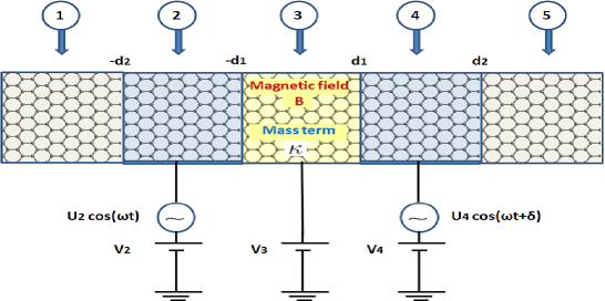
Figure 1: (Color online) Schematic of a graphene monolayer in the presence of an oscillating potential and a magnetic field. Different scattering regions are indicated by an integer j=1,2,3,4,5.

Concerning the applied magnetic field, it is a constant and uniform magnetic field ${\bf B}$ perpendicular to the graphene sheet but confined to a strip of width $2d$. Due to incommensurate effect and interaction with substrate, graphene can develop a mass term in the Hamiltonian. The vector potential that generates our magnetic field can be chosen of the following form

$$\qquad A_{y}(x)=\frac{c}{el_{B}^{2}}\left\{\begin{array}[]{ll}-d_{1},&\hbox{$x<d_{1}$}\\ x,&\hbox{$|x|<d_{1}$}\\ d_{1},&\hbox{$x>d_{1}$}\\ \end{array}\right.$$ (7)

with the magnetic length defined by $l_{B}=\sqrt{\frac{1}{B_{0}}}$ in the unit system $(\hbar=c=e=1)$.

3 Spectral solutions

We emphasize that the system Hamiltonian (1) is composed of two sub-Hamiltonian, $H_{1}$ plays the role of a perturbation term with respect to $H_{0}$. The independence of these Hamiltonians leads to their commutativity $[H_{0},H_{1}]=0$ and therefore the corresponding eigenspinors $\psi$ are the tensor product of two eigenspinor $\psi_{0}$ and $\psi_{1}$ associated with $H_{0}$ and $H_{1}$, respectively i.e. $\psi(x,y,t)=\psi(x,y)\psi(t)$ and the eigenvalue of $H$ is the sum of eigenvalues $E=E_{0}+E_{1}.$ The eigenspinor $\psi$ of the system obeys the equation

$$H\psi(x,y,t)=i\partial_{t}\psi_{j}(x,y,t)$$ (8)

which can be written as

$$\left[E_{0}+U_{j}\cos\left(\omega t+\delta_{j}\Theta(x)\right)\right]\psi_{j}(x,y,t)=i\partial_{t}\psi_{j}(x,y,t).$$ (9)

The integration between $t_{0}=0$ and $t$ gives

$$\psi_{j}(x,y,t)=\psi_{j}(x,y,0)e^{-iE_{0}t}e^{-iU_{j}\sin\left(\omega t+\delta_{j}\Theta(x)\right)/\omega}$$ (10)

where the last term is in the form of $e^{i\alpha_{j}\sin\Phi}$, which can be expanded into trigonometric series as

$$e^{i\alpha_{j}\sin\Phi}=\sum_{m=-\infty}^{+\infty}J_{m}(\alpha_{j})e^{im\Phi}$$ (11)

with $\alpha_{j}=\frac{U_{j}}{\omega}$ and $\Phi=\omega t+\delta_{j}\Theta(x)$. Hence finally we obtain

$$\psi_{j}(x,y,t)=\psi_{j}(x,y,0)e^{-iE_{0}t}\sum_{m=-\infty}^{+\infty}J_{m}(\alpha_{j})e^{im(\omega t+\delta)}$$ (12)

and $C_{m}=J_{m}\left(\alpha_{j}\right)$ satisfies the recurrence relation

$$2mC_{m}=\alpha_{j}\left(C_{m+1}+C_{m-1}\right)$$ (13)

where $J_{m}$ is the $m$-th order Bessel function of the first kind. Using these eigenspinors we readily determine the total energy from (12) to be

$$E=E_{0}+m\omega.$$ (14)

Taking into account energy conservation, the wave packet that describes our carrier in the $j$-th region can be expressed as a linear combination of wave functions at energies $E_{0}+l\omega$ $(l=0,\pm 1,\cdots)$. This is

$$\psi_{j}(x,y,t)=e^{ik_{y}y}\sum^{m,l=+\infty}_{m,l=-\infty}\psi_{j}^{l}(x,y)J_{m-l}\left(\alpha_{j}\right)e^{-i(m-l)\delta_{j}}e^{-iv_{F}(\epsilon+m\varpi)t}$$ (15)

where we have set $\epsilon=\frac{E_{0}}{\upsilon_{F}}$ and $\varpi=\frac{\omega}{\upsilon_{F}}$. Subsequently, the spinor $\psi_{\sf j}^{l}(x,y)$ will be determined in each region $j$.

The Dirac eigenvalue equation in the absence of oscillating potential for the spinor $\psi(x,y)=(\psi_{+},\psi_{-})^{T}$ at energy $E_{0}$ reads

$$H_{0}\psi(x,y)=E_{0}\psi(x,y).$$ (16)

Using the explicit form of $H_{0}$ given by (2) we find

$$\left(\begin{array}[]{cc}v_{j}+\mu&p_{jx}-ip_{y}-iA(x)\\ p_{jx}+ip_{y}+iA(x)&v_{j}-\mu\\ \end{array}\right)\left(\begin{array}[]{c}\psi_{+}\\ \psi_{-}\\ \end{array}\right)=\epsilon\left(\begin{array}[]{c}\psi_{+}\\ \psi_{-}\\ \end{array}\right)$$ (17)

where $v_{j}=\frac{V_{j}}{v_{F}}$ and $\mu=\frac{\kappa}{v_{F}}$ . Due to the translational invariance along the $y$-direction, the two-component pseudospinor can be written as $\psi_{\pm}(x,y)=\varphi_{\pm}(x)e^{ik_{y}y}$. In region $j$ = 1, 2, 4 and 5, we easily obtain the following two linear differential equations

$$\left(p_{jx}-p_{y}-iA(x)\right)\varphi_{-}=(\epsilon-v_{j})\varphi_{+}$$ (18)

$$\left(p_{jx}+p_{y}+iA(x)\right)\varphi_{+}=(\epsilon-v_{j})\varphi_{-}.$$ (19)

In accordance with (15), the general solution in the $j$-th scattering region reads as

$$\psi_{\sf j}(x,y,t) = e^{ik_{y}y}\sum^{m,l=+\infty}_{m,l=-\infty}\left[a_{l}^{j}\left(\begin{array}[]{c}1\\ z_{l}^{j}\end{array}\right)e^{ik^{j}_{l}(x-x_{j})}+b_{l}^{j}\left(\begin{array}[]{c}1\\ -\frac{1}{z_{l}^{j}}\end{array}\right)e^{-ik^{j}_{l}(x-x_{j})}\right]$$ (25)

$$\times J_{m-l}\left(\alpha_{j}\right)e^{-i(m-l)\delta_{j}}e^{-iv_{F}(\epsilon+m\varpi)t}$$

where $s_{l}^{j}=\mbox{sgn}(\epsilon+l\varpi-v_{j})$, the sign again refers to conduction and valence bands, $x_{j}$ are the positions of the interfaces (Figure 1): $x_{1}=x_{2}=-d_{2}$, $x_{3}=-d_{1}$, $x_{4}=d_{1}$, $x_{5}=d_{2}$. Note that, outside the barrier regions where the modulation amplitude is $\alpha_{j}=0$ we have the function $J_{m-l}\left(\alpha_{j}\right)=\delta_{m,l}$. The wave vector is given by

$$k_{l}^{j}=s_{l}^{j}\sqrt{\left(\epsilon-v_{j}+l\varpi\right)^{2}-\left(k_{y}+\frac{d}{l^{2}_{B}}\right)^{2}}$$ (26)

which leads to the corresponding eigenvalues

$$\epsilon-v_{j}+l\varpi=s_{l}^{j}\sqrt{\left(k_{l}^{j}\right)^{2}+\left(k_{y}+\frac{d}{l^{2}_{B}}\right)^{2}}$$ (27)

with the magnetic length defined by $l_{B}=\sqrt{1/B_{0}}$ and the complex parameter $z_{l}^{j}$ is

$$z_{l}^{j}=s_{l}^{j}\frac{k^{j}_{l}+i\left(k_{y}+\frac{d}{l^{2}_{B}}\right)}{\sqrt{\left(k_{l}^{j}\right)^{2}+\left(k_{y}+\frac{d}{l^{2}_{B}}\right)^{2}}}=s_{l}^{j}e^{\textbf{\emph{i}}\phi_{l}^{j}}$$ (28)

$\phi_{l}^{j}=\tan^{-1}(k_{y}/k_{l}^{j})$ and the parameter $d$ is defined by

$$d=\left\{\begin{array}[]{ll}d_{1},&\hbox{$x<-d_{1}$}\\ -d_{1},&\hbox{$x>d_{1}$.}\\ \end{array}\right.$$ (29)

Let us proceed to write down the solution in the intermediate zone ${j=3}$ $(-d_{1}<x<d_{1})$ containing the mass term in addition to a perpendicular magnetic field. To diagonalize the corresponding Hamiltonian we introduce the usual boson operators

$$a_{l}=\frac{l_{B}}{\sqrt{2}}\left(\partial_{x}+k_{y}+\frac{x}{l_{B}^{2}}\right),\qquad a_{l}^{\dagger}=\frac{l_{B}}{\sqrt{2}}\left(-\partial_{x}+k_{y}+\frac{x}{l_{B}^{2}}\right)$$ (30)

which satisfy the commutation relation $\left[a_{l},a_{k}^{\dagger}\right]=\delta_{lk}$. In terms of $a_{l}$ and $a_{l}^{\dagger}$, equation (17) reads

$$\left(\begin{array}[]{cc}v_{3}+\mu&-i\frac{\sqrt{2}}{l_{B}}a_{l}\\ i\frac{\sqrt{2}}{l_{B}}a_{l}^{\dagger}&v_{3}-\mu\\ \end{array}\right)\left(\begin{array}[]{c}\varphi_{l,1}\\ \varphi_{l,2}\\ \end{array}\right)=(\epsilon+l\varpi)\left(\begin{array}[]{c}\varphi_{l,1}\\ \varphi_{l,2}\\ \end{array}\right)$$ (31)

or in its explicit form

$$-i\frac{\sqrt{2}}{l_{B}}a_{l}\varphi_{l,2}=\left(\epsilon+l\varpi-v_{3}-\mu\right)\varphi_{l,1}$$ (32)

$$i\frac{\sqrt{2}}{l_{B}}a_{l}^{\dagger}\varphi_{l,1}=\left(\epsilon+l\varpi-v_{3}+\mu\right)\varphi_{l,2}.$$ (33)

Combining the above equations, we obtain for $\varphi_{l,1}$

$$\left(\left(\epsilon+l\varpi-v_{3}\right)^{2}-\mu^{2}\right)\varphi_{l,1}=\frac{2}{l_{B}^{2}}a_{l}a_{l}^{\dagger}\varphi_{l,1}.$$ (34)

It is clear that $\varphi_{l,1}$ is an eigenstate of the number operator $\widehat{N}=a_{l}^{\dagger}a_{l}$ and therefore we identify $\varphi_{l,1}$ with the eigenstates of the harmonic oscillator $|n-1\rangle$, namely

$$\varphi_{l,1}\sim\mid n-1\rangle$$ (35)

and the associated eigenvalues are

$$\epsilon-v_{3}+l\varpi=\pm\frac{1}{l_{B}}\sqrt{\left(\mu l_{B}\right)^{2}+2n}.$$ (36)

Finally, the solution in region $j=3$ can be expressed in accordance with equation (15), as follows

$$\psi_{\sf 3}(x,y,t)=e^{ik_{y}y}\sum^{l=+\infty}_{l=-\infty}\left(a_{l}^{3}\varphi^{+}_{l}+b_{l}^{3}\varphi^{-}_{l}\right)e^{-iv_{F}(\epsilon+l\varpi)t}$$ (37)

where $\varphi^{\pm}_{l}$ are given by

$$\varphi^{\pm}_{l} = \left(\begin{array}[]{c}\sqrt{\frac{\epsilon_{l,n}\pm\mu}{\epsilon_{l,n}}}D_{\left[(\epsilon_{l,n}l_{B})^{2}-(\mu l_{B})^{2}\right]/2-1}\left[\pm\sqrt{2}\left(\frac{1}{l_{B}}(x-x_{3})+k_{y}l_{B}\right)\right]\\ \pm i\frac{\sqrt{2/l_{B}^{2}}}{\sqrt{\epsilon_{l,n}(\epsilon_{l,n}\pm\mu)}}D_{\left[(\epsilon_{l,n}l_{B})^{2}-(\mu l_{B})^{2}\right]/2}\left[\pm\sqrt{2}\left(\frac{1}{l_{B}}(x-x_{3})+k_{y}l_{B}\right)\right]\\ \end{array}\right)$$ (40)

In the forthcoming analysis, we will see how the obtained results so far can be applied to deal with different issues. More precisely, we will focus on the transmission probability for different channels.

4 Transmission probability

Based on different considerations, we study interesting features of our system in terms of the corresponding transmission probability. Before doing so, let us simplify our writing using the following shorthand notation

$$A_{l,n}^{\pm}=\sqrt{\frac{\epsilon_{l,n}\pm\mu}{\epsilon_{l,n}}}$$ (41)

$$B_{l,n}^{\pm}=\frac{\sqrt{2/l_{B}^{2}}}{\sqrt{\epsilon_{l,n}(\epsilon_{l,n}\pm\mu)}}$$ (42)

$$\eta_{1,l}^{\pm}=D_{\left[(\epsilon_{l,n}l_{B})^{2}-(\mu l_{B})^{2}\right]/2-1}\left[\pm\sqrt{2}\left(k_{y}l_{B}\right)\right]$$ (43)

$$\xi_{1,l}^{\pm}=D_{\left[(\epsilon_{l,n}l_{B})^{2}-(\mu l_{B})^{2}\right]/2}\left[\pm\sqrt{2}\left(k_{y}l_{B}\right)\right]$$ (44)

$$\eta_{2,l}^{\pm}=D_{\left[(\epsilon_{l,n}l_{B})^{2}-(\mu l_{B})^{2}\right]/2-1}\left[\pm\sqrt{2}\left(\frac{2d_{1}}{l_{B}}+k_{y}l_{B}\right)\right]$$ (45)

$$\xi_{2,l}^{\pm}=D_{\left[(\epsilon_{l,n}l_{B})^{2}-(\mu l_{B})^{2}\right]/2}\left[\pm\sqrt{2}\left(\frac{2d_{1}}{l_{B}}+k_{y}l_{B}\right)\right].$$ (46)

Realizing that $\{e^{imv_{F}\varpi t}\}$ are orthogonal, we obtain set of simultaneous equations emanating from the boundary conditions at $x=-d_{2}$

$$a_{m}^{1}+b_{m}^{1}=\sum^{l=\infty}_{l=-\infty}\left(a^{2}_{l}+b^{2}_{l}\right)J_{m-l}\left(\frac{u_{2}}{\varpi}\right)$$ (47)

$$a_{m}^{1}z_{m}^{1}-b_{m}^{1}\frac{1}{z_{m}^{1}}=\sum^{l=\infty}_{l=-\infty}\left(a^{2}_{l}z_{l}^{2}-b^{2}_{l}\frac{1}{z_{l}^{2}}\right)J_{m-l}\left(\frac{u_{2}}{\varpi}\right)$$ (48)

similarly at $x=-d_{1}$

$$a^{3}_{m}A^{+}_{m,n}\eta_{1,m}^{+}+b^{3}_{m}A^{-}_{m,n}\eta_{1,m}^{-}=\sum^{l=\infty}_{l=-\infty}\left(a^{2}_{l}e^{ik_{l}^{2}(d_{2}-d_{1})}+b^{2}_{l}e^{-ik_{l}^{2}(d_{2}-d_{1})}\right)J_{m-l}\left(\frac{u_{2}}{\varpi}\right)$$ (49)

$$a^{3}_{m}iB^{+}_{m,n}\xi_{1,m}^{+}-b^{3}_{m}iB^{-}_{m,n}\xi_{1,m}^{-}=\sum^{l=\infty}_{l=-\infty}\left(a^{2}_{l}z_{l}^{2}e^{ik_{l}^{2}(d_{2}-d_{1})}-b^{2}_{l}\frac{1}{z_{l}^{2}}e^{-ik_{l}^{2}(d_{2}-d_{1})}\right)J_{m-l}\left(\frac{u_{2}}{\varpi}\right)$$ (50)

and at $x=d_{1}$

$$a^{3}_{m}A^{+}_{m,n}\eta_{2,m}^{+}+b^{3}_{m}A^{-}_{m,n}\eta_{2,m}^{-}=\sum^{l=\infty}_{l=-\infty}\left(a^{4}_{l}+b^{4}_{l}\right)J_{m-l}\left(\frac{u_{4}}{\varpi}\right)e^{-i(m-l)\delta}$$ (51)

$$a^{3}_{m}iB^{+}_{m,n}\xi_{2,m}^{+}-b^{3}_{m}iB^{-}_{m,n}\xi_{2,m}^{-}=\sum^{l=\infty}_{l=-\infty}\left(a^{4}_{l}z_{l}^{4}-b^{4}_{l}\frac{1}{z_{l}^{4}}\right)J_{m-l}\left(\frac{u_{4}}{\varpi}\right)e^{-i(m-l)\delta}.$$ (52)

However, at $x=d_{2}$ we have

$$a_{m}^{5}+b_{m}^{5}=\sum^{l=\infty}_{l=-\infty}\left(a^{4}_{l}e^{ik_{l}^{4}(d_{2}-d_{1})}+b^{4}_{l}e^{-ik_{l}^{4}(d_{2}-d_{1})}\right)J_{m-l}\left(\frac{u_{4}}{\varpi}\right)e^{-i(m-l)\delta}$$ (53)

$$a_{m}^{5}z_{m}^{5}-b_{m}^{5}\frac{1}{z_{m}^{5}}=\sum^{l=\infty}_{l=-\infty}\left(a^{4}_{l}z_{l}^{4}e^{ik_{l}^{4}(d_{2}-d_{1})}-b^{4}_{l}\frac{1}{z_{l}^{4}}e^{-ik_{l}^{4}(d_{2}-d_{1})}\right)J_{m-l}\left(\frac{u_{4}}{\varpi}\right)e^{-i(m-l)\delta}.$$ (54)

As Dirac electrons pass through a region subject to time-harmonic potentials, transitions from the central band to sidebands (channels) at energies $\epsilon\pm m\varpi$ $(m=0,1,2,\cdots)$ occur as electrons ex- change energy quanta with the oscillating field. It should be noted that (47-54) can be written in a compact form as

$$\left(\begin{array}[]{c}\Xi_{1}\\ \Xi_{1}^{{}^{\prime}}\\ \end{array}\right)=\left(\begin{array}[]{cc}{\mathbb{M}11}&{\mathbb{M}12}\\ {\mathbb{M}21}&{\mathbb{M}22}\\ \end{array}\right)\left(\begin{array}[]{c}\Xi_{5}\\ \Xi_{5}^{{}^{\prime}}\\ \end{array}\right)={\mathbb{M}}\left(\begin{array}[]{c}\Xi_{5}\\ \Xi_{5}^{{}^{\prime}}\\ \end{array}\right)$$ (63)

where the total transfer matrix ${\mathbb{M}}={\mathbb{M}(1,2)}\cdot{\mathbb{M}(2,3)}\cdot{\mathbb{M}(3,4)}\cdot{\mathbb{M}(4,5)}$ and ${\mathbb{M}(j,j+1)}$ are transfer matrices that couple the wave function in the $j$-th region to that in the $(j+1)$-th one. These are explicitly defined by

$${\mathbb{M}(1,2)}=\left(\begin{array}[]{cc}{\mathbb{I}}&{\mathbb{I}}\\ {\mathbb{N}^{+}}&{\mathbb{N}^{-}}\\ \end{array}\right)^{-1}\left(\begin{array}[]{cc}{\mathbb{C}}&{\mathbb{C}}\\ {\mathbb{G}^{+}}&{\mathbb{G}^{-}}\\ \end{array}\right)$$ (68)

$${\mathbb{M}(2,3)}=\left(\begin{array}[]{cc}{\mathbb{Y}_{1}^{+}}&{\mathbb{Y}_{1}^{-}}\\ {\mathbb{Y}_{2}^{+}}&{\mathbb{Y}_{2}^{-}}\\ \end{array}\right)^{-1}\left(\begin{array}[]{cc}{\mathbb{Q}_{1}^{+}}&{\mathbb{Q}_{1}^{-}}\\ {\mathbb{F}_{1}^{+}}&{\mathbb{F}_{1}^{-}}\\ \end{array}\right)$$ (73)

$${\mathbb{M}(3,4)}=\left(\begin{array}[]{cc}{\mathbb{Q}_{2}^{+}}&{\mathbb{Q}_{2}^{-}}\\ {\mathbb{F}_{2}^{+}}&{\mathbb{F}_{2}^{-}}\\ \end{array}\right)^{-1}\left(\begin{array}[]{cc}{\mathbb{D}_{1}}&{\mathbb{D}_{1}}\\ {\mathbb{D}_{2}^{+}}&{\mathbb{D}_{2}^{-}}\\ \end{array}\right)$$ (78)

$${\mathbb{M}(4,5)}=\left(\begin{array}[]{cc}{\mathbb{K}_{1}^{+}}&{\mathbb{K}_{1}^{-}}\\ {\mathbb{K}_{2}^{+}}&{\mathbb{K}_{2}^{-}}\\ \end{array}\right)^{-1}\left(\begin{array}[]{cc}{\mathbb{I}}&{\mathbb{I}}\\ {\mathbb{E}^{+}}&{\mathbb{E}^{-}}\\ \end{array}\right)$$ (83)

whose matrix elements are expressed as

$$\left({\mathbb{N}^{\pm}}\right)_{m,l}=\pm\left(z_{m}^{1}\right)^{\pm 1}\delta_{m,l}$$ (84)

$$\left({\mathbb{C}}\right)_{m,l}=J_{m-l}\left(\frac{u_{2}}{\varpi}\right)$$ (85)

$$\left({\mathbb{G}^{\pm}}\right)_{m,l}=\pm(z_{l}^{1})^{\pm 1}J_{m-l}\left(\frac{u_{2}}{\varpi}\right)$$ (86)

$$\left({\mathbb{Y}_{1}^{\pm}}\right)_{m,l}=e^{\pm ik_{l}^{2}(d_{2}-d_{1})}J_{m-l}\left(\frac{u_{2}}{\varpi}\right)$$ (87)

$$\left({\mathbb{Y}_{2}^{\pm}}\right)_{m,l}=\pm(z_{l}^{2})^{\pm 1}e^{\pm ik_{l}^{2}(d_{2}-d_{1})}J_{m-l}\left(\frac{u_{2}}{\varpi}\right)$$ (88)

$$\left({\mathbb{Q}_{\tau}^{\pm}}\right)_{m,l}=A_{m,n}^{\pm}\eta_{\tau,m}^{\pm}\delta_{m,l}$$ (89)

$$\left({\mathbb{F}_{\tau}^{\pm}}\right)_{m,l}=\pm iB_{m,n}\xi_{\tau,m}^{\pm}\delta_{m,l}$$ (90)

$$\left({\mathbb{D}_{1}}\right)_{m,l}=J_{m-l}\left(\frac{u_{4}}{\varpi}\right)e^{\left(-i(m-l)\delta\right)}$$ (91)

$$\left({\mathbb{D}_{2}^{\pm}}\right)_{m,l}=\pm(z_{l}^{4})^{\pm 1}J_{m-l}\left(\frac{u_{4}}{\varpi}\right)e^{\left(-i(m-l)\delta\right)}$$ (92)

$$\left({\mathbb{K}_{1}^{\pm}}\right)_{m,l}=e^{\pm ik_{l}^{4}(d_{2}-d_{1})}J_{m-l}\left(\frac{u_{4}}{\varpi}\right)e^{\left(-i(m-l)\delta\right)}$$ (93)

$$\left({\mathbb{K}_{2}^{\pm}}\right)_{m,l}=\pm(z_{l}^{4})^{\pm 1}e^{\pm ik_{l}^{4}(d_{2}-d_{1})}J_{m-l}\left(\frac{u_{4}}{\varpi}\right)e^{\left(-i(m-l)\delta\right)}$$ (94)

$$\left({\mathbb{E}^{\pm}}\right)_{m,l}=\pm\left(z_{m}^{5}\right)^{\pm 1}\delta_{m,l}$$ (95)

and the unit matrix is denoted by ${\mathbb{I}}$. We assume an electron propagating from left to right with quasienergy $\epsilon$. Then, $\tau\in\{1,2\}$, $\Xi_{1}=\{a_{m}^{1}\}=\{\delta_{m,0}\}$ and $\Xi_{5}^{{}^{\prime}}=\{b_{m}^{5}\}$ is the null vector, whereas $\Xi_{5}=\{a_{m}^{5}\}=\{t_{m}\}$ and $\Xi_{1}^{{}^{\prime}}=\{b_{m}^{1}\}=\{r_{m}\}$ are vectors associated with transmitted waves and reflected waves, respectively. From the above considerations, one can easily obtain the relation

$$\Xi_{5}=\left({\mathbb{M}11}\right)^{-1}\cdot\Xi_{1}$$ (96)

which is equivalent to the explicit form

$$\left(\begin{array}[]{cc}t_{-N}\\ .\\ .\\ t_{-1}\\ t_{0}\\ t_{1}\\ .\\ .\\ t_{N}\\ \end{array}\right)=\left({\mathbb{M}11}\right)^{-1}\left(\begin{array}[]{cc}0\\ 0\\ 0\\ 0\\ 1\\ 0\\ 0\\ 0\\ 0\\ \end{array}\right)$$ (115)

The minimum number $N$ of sidebands that need to be taken is determined by the strength of the oscillating potential, $N>\mbox{max}\left(\frac{u_{2}}{\varpi},\frac{u_{4}}{\varpi}\right)$ [10]. Then the infinite series for the transmission $T$ can be truncated considering only a finite number of terms starting from $-N$ up to $N$. Furthermore, analytical results are obtained if we pick up small values of $\alpha_{2}=\frac{u_{2}}{\varpi}$, $\alpha_{4}=\frac{u_{4}}{\varpi}$ and include only the first two sidebands at energies $\epsilon\pm m\varpi$ along with the central band at energy $\epsilon$. This gives

$$t_{-N+k}={\mathbb{M}^{{}^{\prime}}}\left[k+1,N+1\right)]$$ (116)

where $k=0,1,2,\cdots,2N$ and ${\mathbb{M}^{{}^{\prime}}}$ denotes the inverse matrix $\left({\mathbb{M}11}\right)^{-1}$.

Using the reflected $J_{\sf{ref}}$ and transmitted $J_{\sf{tra}}$ currents to write the reflection and transmission coefficients $R_{l}$ and $T_{l}$ as

$$T_{l}=\frac{|J_{{\sf{tra}},l}|}{|J_{{\sf{inc}},0}|},\qquad R_{l}=\frac{|J_{{\sf{ref}},l}|}{|J_{\sf{inc,0}}|}$$ (117)

where $T_{l}$ is the transmission coefficient describing the scattering of an electron with incident quasienergy $\epsilon$ in the region 1 into the sideband with quasienergy $\epsilon+l\varpi$ in the region 5. Thus, the rank of the transfer matrix $({\mathbb{M}})$ increases with the amplitude of the time-oscillating potential. The total transmission coefficient for quasienergy $\epsilon$ is

$$T=\sum_{l=-\infty}^{l=+\infty}T_{l}.$$ (118)

The electrical current density $J$ corresponding to our system can be derived to be

$$J=v_{F}\psi^{\dagger}\sigma_{x}\psi$$ (119)

which explicitly reads as

$$J_{{\sf{inc}},0}=v_{F}\left(z_{0}^{1}+\left(z_{0}^{1}\right)^{\ast}\right)$$ (120)

$$J_{{\sf{ref}},l}=v_{F}\left(b_{l}^{1}\right)^{\ast}b_{l}^{1}\left(z_{l}^{1}+\left(z_{l}^{1}\right)^{\ast}\right)$$ (121)

$$J_{{\sf{tra}},l}=v_{F}\left(a_{l}^{5}\right)^{\ast}a_{l}^{5}\left(z_{l}^{5}+\left(z_{l}^{5}\right)^{\ast}\right).$$ (122)

The transmission coefficient for the sideband, $T_{l}$, is real and corresponds to propagating waves. It can be written as

$$T_{l}=\frac{s_{l}^{5}k^{5}_{l}}{s_{0}^{1}k^{1}_{0}}\frac{\left[\left(k^{1}_{0}\right)^{2}+\left(k_{y}-\frac{d_{1}}{l_{B}^{2}}\right)^{2}\right]^{\frac{1}{2}}}{\left[\left(k^{5}_{l}\right)^{2}+\left(k_{y}+\frac{d_{1}}{l_{B}^{2}}\right)^{2}\right]^{\frac{1}{2}}}\mid t_{l}^{5}\mid^{2}.$$ (123)

Now using the energy conservation to simplify $T_{l}$ to

$$T_{l}=\frac{k^{5}_{l}}{k^{1}_{0}}\left(1-\frac{s_{l}^{5}l\varpi}{\sqrt{\left(k^{5}_{l}\right)^{2}+\left(k_{y}+\frac{d_{1}}{l_{B}^{2}}\right)^{2}}}\right)\mid t_{l}^{5}\mid^{2}.$$ (124)

To explore the above results and go deeply in order to underline our system behavior, we will pass to the numerical analysis. For this, we will focus only on few channels and choose different configurations of the physical parameters.

5 Discussions

We discuss the numerical results for both the reflection and transmission coefficients, which are shown in Figures 2, 3, 4, 5, 6, 7, 8, 9 for different values of the parameters ($\epsilon$, $v_{2}$, $v_{3}$, $d_{1}$, $d_{2}$, $\alpha_{2}$, $\alpha_{4}$, $\delta$, $\mu$). To start with we point out the efficiency and accuracy of our computational method and compare our results with those reported in the literature. As a matter of fact, Figure 2(a) and Figure 2(b) reproduce exactly the results obtained in [24] for single barrier and [25] for double barrier, respectively, with the proper choice of parameters. Note that reference [24] was the first to treat the confinement of Dirac fermions by an inhomogeneous magnetic field. These polar graphs show the transmission as a function of the incidence angle, the outermost circle corresponds to full transmission, $T_{0}=1$, while the origin of this plot represents zero transmission, i.e. total reflection. For energies satisfying the condition $(\epsilon+l\varpi)l_{B}\leq\frac{d_{1}}{l_{B}}$, we obtain total reflection [24, 25]. This is equivalent to the condition on the incidence angle $\phi<\phi_{c}$ where $\phi_{c}$ is the critical angle given by

$$\phi_{c}=\sin^{-1}\left(1-\frac{2d}{(\epsilon+l\varpi)l^{2}_{B}}\right)$$ (125)

which is analogous to the case of light propagation from a refringent medium to a less refringent one.

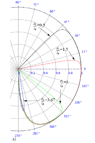
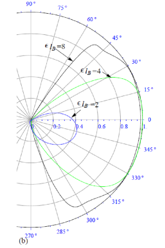
Figure 2: (Color online) Polar plot showing transmission probability (transmission $T_{0}$ ($l$=0)) as a function of angle $\phi_{0}^{1}$ for different values of the parameters. (a): $\frac{d_{1}}{l_{B}}=\{0.5,1.5,3,3.67\}$, $\epsilon l_{B}=3.7$, $\alpha_{2}=\alpha_{4}=0$, $\delta=0$, $\frac{d_{2}}{l_{B}}=\frac{d_{1}}{l_{B}}$, $v_{2}l_{B}=v_{4}l_{B}=0$, $\mu l_{B}=0$ and $v_{3}l_{B}=0$. (b): $\epsilon l_{B}=\{0.6,2,4,8\}$, $\frac{d_{1}}{l_{B}}=0.5$, $\alpha_{2}=\alpha_{4}=0$, $\delta=0$, $\frac{d_{2}}{l_{B}}=0.6$, $v_{2}l_{B}=v_{4}l_{B}=0.5$, $\mu l_{B}=1$ and $v_{3}l_{B}=0.4$ .

After a satisfactory confirmation that our numerical approach reproduced published results, we plot the transmission versus the phase shift $\delta$ in the presence temporal barrier oscillations for the cases $\alpha=\alpha_{2}=\alpha_{4}$ and $\alpha=\alpha_{2}=2\alpha_{4}$. Figure 3 illustrates the variation of the transmission coefficient $T_{0}$ as a function of the phase shift $\delta$ for various harmonic amplitudes $\alpha$ ($0\leq\alpha\leq 0.99$). The first point to emphasize is that both plots in Figure 3 are periodic with period $2\pi$, which is obvious. For $\alpha=0$, the transmission does not depend on the phase shift since the vibration amplitude has been set to zero. For $\alpha=\alpha_{2}=\alpha_{4}$, the transmission varies sinusoidally between 0 and 1, the maximum for different plots does not change for various values of $\alpha$ (Figure 3(a)). However, when the harmonic oscillation amplitudes are not equal ($\alpha_{2}\neq\alpha_{4}$), we observe that there is a remarkable change in the evolution of $T_{0}$ versus $\delta$. We illustrate this situation by selecting $\alpha_{2}=2\alpha_{4}$ then one can see that as long as such difference increases we observe a drastic change in the transmission from full transmission (total transmission) to zero transmission (total reflection), see Figure 3(b).

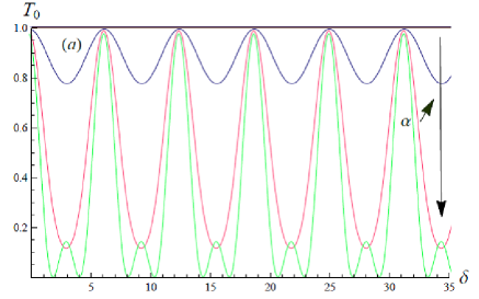
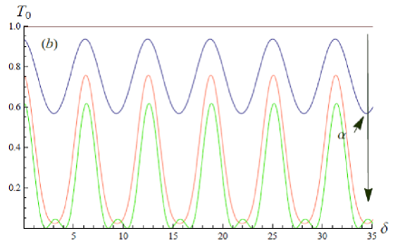
Figure 3: (Color online) The transmission coefficient $T_{0}$ as function of phase shift $\delta$ through graphene double barriers for fixed values $\epsilon l_{B}$, $k_{y}l_{B}$, $\frac{d_{1}}{l_{B}}$, $\frac{d_{2}}{l_{B}}$, $\mu l_{B}$, $v_{3}l_{B}$, $\varpi l_{B}$ and $v_{2}l_{B}=v_{4}l_{B}$ but for different values of $\alpha$. We used $\epsilon l_{B}=25$, $k_{y}l_{B}=2$, $\frac{d_{1}}{l_{B}}=0.3$, $\frac{d_{2}}{l_{B}}=1.35$, $\mu l_{B}=4$, $v_{3}l_{B}=4$, $\varpi l_{B}=2$ and $v_{2}l_{B}=v_{4}l_{B}=6$ and $\alpha$ varies from $0$ to $0.99$. (a): $\alpha=\alpha_{2}=\alpha_{4}$, (b): $\alpha=\alpha_{2}=2\alpha_{4}$

Let us now demonstrate through Figure 4 how the first sideband transmissions $T_{1}$ and $T_{-1}$ vary as function of the phase shift $\delta$. It is clearly seen that the central transmission $T_{0}$ behaves sinusoidally but at some value of $\alpha$ we observe that $T_{0}$ changes its behavior and becomes sharply peaked. $T_{1}$ and $T_{-1}$ show also sinusoidal behaviors with non-symmetric double humps in regions where $T_{0}$ is suppressed. However, one can see that there is a symmetry between the two double humps of the transmissions $T_{1}$ and $T_{-1}$.

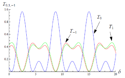
Figure 4: (Color online) Graphs depicting the transmission probabilities as function of phase $\delta$ for graphene double barriers with $\varpi l_{B}=8$, $\alpha_{2}=\alpha_{4}=0.8$, $\epsilon l_{B}=25$, $k_{y}l_{B}=2$, $\frac{d_{1}}{l_{B}}=0.3$, $\frac{d_{2}}{l_{B}}=1.35$, $\mu l_{B}=4$, $v_{3}l_{B}=4$ and $v_{2}l_{B}=v_{4}l_{B}=6$.

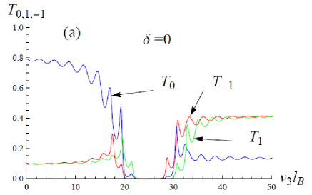
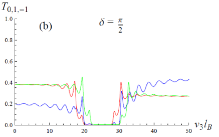
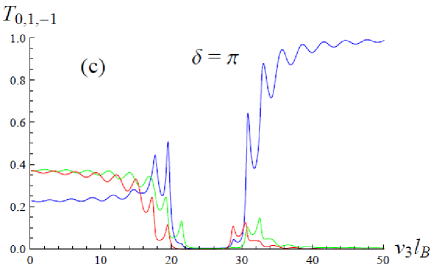
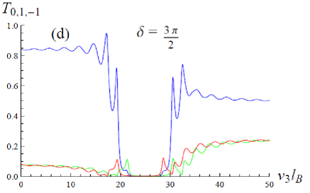
Figure 5: (Color online) Graphs depicting the transmission probabilities as function of potential $v_{3}l_{B}$ for the monolayer graphene barriers with $\frac{d_{2}}{l_{B}}=1.5$, $\frac{d_{1}}{l_{B}}=0.5$, $v_{2}l_{B}=v_{4}l_{B}=4$, $\epsilon l_{B}=25$, $k_{y}l_{B}=2$, $\mu l_{B}=4$, $\varpi l_{B}=2$, $\alpha_{2}=\alpha_{4}=0.5$ and $\delta=\{0,\frac{\pi}{2},\pi,\frac{3\pi}{2}\}$. $T_{0}$ (color blue), $T_{-1}$ (color red) and $T_{1}$ (color green).

Now we will study how the three bands: central and two lateral ones, vary depending on the phase difference of the oscillating potentials in the intermediate region (Figure 5). For different phase shifts, the transmissions of side bands $T_{1}$ and $T_{-1}$ are dominant either before or after the bowl centered region in the propagation energy $\epsilon l_{B}$. In the vicinity of this bowl, one of the two transmissions is more symmetrical with respect to a vertical axis passing through the energy $\epsilon l_{B}$. The degree of dominance of the transmissions $T_{1}$ and $T_{-1}$ is less pronounced in the case of advanced phase quadrature $\delta=\frac{\pi}{2}$ (Figure 5(b)). But they are more dominant in the case of $\delta=0$ and $\delta=\frac{3\pi}{2}$ where the potential $v_{3}l_{B}$ is greater than the propagation energy $\epsilon l_{B}$ and are less dominant when $v_{3}l_{B}$ is less than the propagation energy $\epsilon l_{B}$. The behavior of the transmission side bands differs in the case of opposite phase shift $\delta=\pi$. On the other hand, the transmission of the central band, for different phase shifts, has also a dominance of either side of the high potential $v_{3}l_{B}$ than the propagation energy $\epsilon l_{B}$ or the other side where the potential $v_{3}l_{B}$ is small than the same energy.

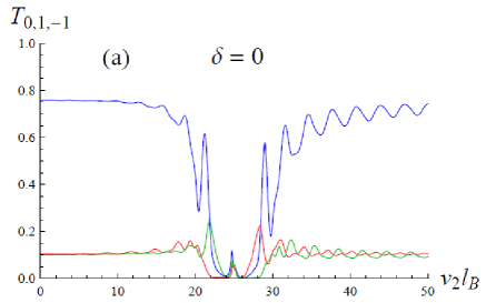
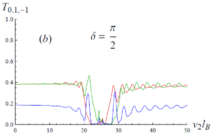
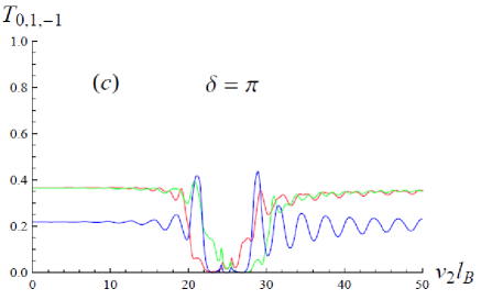
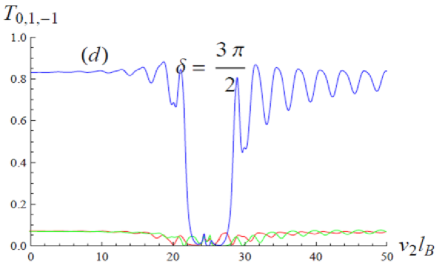
Figure 6: (Color online) Graphs depicting the transmission probabilities as function of potential $v_{2}l_{B}$ for monolayer graphene barriers with $\alpha_{2}=\alpha_{4}=0.5$, $\varpi l_{B}=2$, $\epsilon l_{B}=25$, $k_{y}l_{B}=2$, $\frac{d_{1}}{l_{B}}=0.5$, $\frac{d_{2}}{l_{B}}=1.6$, $\mu l_{B}=4$, $v_{3}l_{B}=4$ and $\delta=\{0,\frac{\pi}{2},\pi,\frac{3\pi}{2}\}$. $T_{0}$ (color blue), $T_{-1}$ (color red) and $T_{1}$ (color green).

Figure 6 is similar to Figure 5, the only main difference to be noted is that there is presence of peaks in the bowl centered around the value $v_{2}=\epsilon$ and $T_{0,-1,1}$ heights are in the same order either before or after the bowl. These peaks are due to the resonances between the bound states existing in both sides of the regions subject to the potential $v_{3}$. This behavior is normal if we keep in mind that our double barrier is composed of two successive squares with the same potential $v_{2}$ and width $(d_{2}-d_{1})$ separated by the width $2d_{1}$ corresponding to the intermediate region.

Figure 7 shows the transmission probability as a function of the incident energy of electrons for $v_{2}l_{B}=25$, $k_{y}l_{B}=2$, $\frac{d_{1}}{l_{B}}=0.5$, $\frac{d_{2}}{l_{B}}=1.5$, $\mu l_{B}=4$, $v_{3}l_{B}=4$ and different amplitudes of the oscillating barrier without shift $\delta=0$. Resonant peaks are narrow and could have important applications in high-speed devices based on graphene as has been suggested previously [10]. The evolution of the central and two lateral transmission bands depend on the width of the double barrier potential over time accompanied by a magnetic field (Figures 7(a), 7(b)).

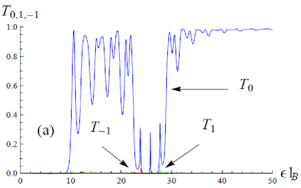
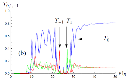
Figure 7: (Color online) Graphs depicting the transmission probabilities as function of energy $\epsilon l_{B}$ for the monolayer graphene barriers with $\alpha_{2}=\alpha_{4}=\{0.08,0.5\}$, $v_{2}l_{B}=25$, $k_{y}l_{B}=2$, $\frac{d_{1}}{l_{B}}=0.5$, $\frac{d_{2}}{l_{B}}=1.5$, $\mu l_{B}=4$, $v_{3}l_{B}=4$, $\varpi l_{B}=2$ and $\delta=0$.

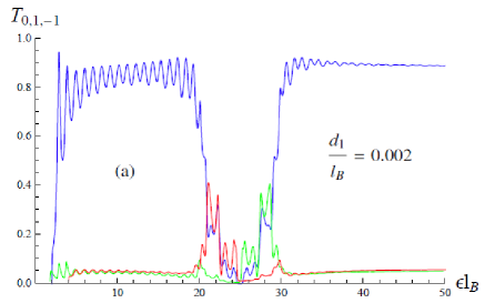
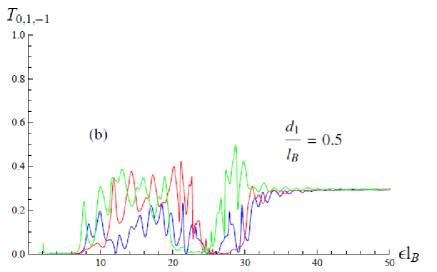
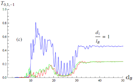
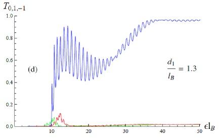
Figure 8: (Color online) Graphs depicting the transmission probabilities as function of energy $\epsilon l_{B}$ for monolayer graphene barriers with $\alpha_{2}=\alpha_{4}=0.99$, $\frac{d_{1}}{l_{B}}=\{0,0.02,0.5,1,1.3\}$, $v_{2}l_{B}=25$, $k_{y}l_{B}=2$, $\frac{d_{2}}{l_{B}}=1.5$, $\mu l_{B}=4$, $v_{3}l_{B}=4$, $\varpi l_{B}=2$ and $\delta=\pi$. $T_{0}$ (color blue), $T_{-1}$ (color red) and $T_{1}$ (color green).

Figure 8 presents transmission versus the system energy for different widths. Indeed, we observe that in Figure 8(a) as long as the width is very small the central band is dominant and therefore the transmission becomes total independently of the applied potential. Figure 8(b) is obtained by increasing the width $d$ up to some value, one can see the dominance of the two sideband transmissions compared to central band one. We notice that these two sideband transmissions are symmetrical with respect to an axis of symmetry located at double barrier potential $v_{2}$ of the propagation energy. After increasing the width $d$, we end up with Figure 8(c), which is similar to the last one but this time with dominance of the central band transmission. It is clearly seen that the total transmission is less than or equal to unity. In Figure 8(d), the central band transmission recovers its dominance but evanescence of two sideband transmissions.

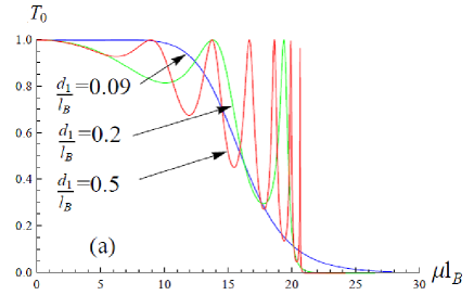
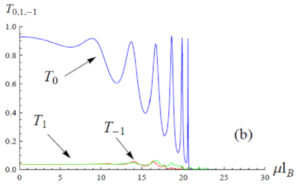
Figure 9: (Color online) Graphs depicting the transmission total $T$ as function of energy gap $\mu l_{B}$ for the monolayer graphene barriers with: $\frac{d_{2}}{l_{B}}=0.7$, $v_{2}l_{B}=v_{4}l_{B}=4$, $\epsilon l_{B}=25$, $k_{y}l_{B}=2$, $v_{3}l_{B}=4$, $\varpi l_{B}=2$, $\alpha_{2}=\alpha_{4}=0$ and $\delta=0$ (a): $\frac{d_{1}}{l_{B}}=\{0.09,0.2,0.5\}$, $\alpha_{2}=\alpha_{4}=0$ and $\delta=0$. (b): $\frac{d_{1}}{l_{B}}=0.5$, $\alpha_{2}=\alpha_{4}=0.7$ and $\delta=\frac{3\pi}{4}$ .

Figure 9 is intended to see the influence of increasing the width of the intermediate zone, where there is a magnetic field, on the dominant transmission central depending on the mass term $\mu l_{B}$ that in the intermediate region. The distance $d_{2}$ remains constant which means that the widths of regions 2 and 4 decrease if $d_{1}$ increases. Figure 9(a) shows that progressively as the distance $d_{1}$ increases, the central transmission acquires resonances which clamp by increasing amplitudes whose upper peaks correspond to a total transmission (maximum). The maximum value of $T_{0}(\mu)$ is the unit since $\alpha=\alpha_{2}=\alpha_{4}=0$. In Figure 9(b) for $\alpha\neq 0$ the maximum value of $T_{0}(\mu)$ decreases at the expense of transmission sidebands $T_{-1,1}(\mu)$. We note that the sum of the three transmissions $T_{0,-1,1}(\mu)$ converges whenever towards unity.

6 Conclusion

In this present work, we studied the transmission probability in graphene through double barriers with periodic potential in time. The double barrier contains an intermediate region has a magnetic field with a mass term, but the two temporal harmonic potentials with different amplitudes and phase shifted are applied one hand and on the other in both regions restricting the intermediate region. This panoply of potential makes our studied system rich in terms of physical states whose energy is doubling quantified by the pair $(n,l)$ extensively degenerated with a very large number of modes.

To identify the difficulties posed, we made the problem by adequate truncation to reduce all modes in three modes one central and two lateral indexed by $(0,-1,1$). We tried to study the influence of various parameters such as ($\epsilon$, $v_{2}$, $v_{3}$, $d_{1}$, $d_{2}$, $\alpha_{2}$, $\alpha_{4}$, $\delta$, $\mu$) on the transmission probability and highlight some properties of the system under consideration. The critical angle (see (125)), at which total reflection sets in, showed in an efficient manner the analogy between the propagation of Dirac fermions in our system and the propagation of the light of a more refractive homogeneous isotropic transparent medium a less refractive one. This built an interesting bridge between two areas of physics such matter and light.

The transmission probability $T_{0}(\delta)$ is obtained to be harmonic with frequency proportional to $\varpi$ of time dependent amplitude $\alpha$. We observed that as long as the amplitude $\alpha$ of time-harmonic potentials is increased $T_{0}(\mu)$ is decreased at the expense of lateral transmissions $T_{-1,1}(\mu)$ and the three transmission $T_{0,-1,1}(\mu)$ behaves in a complementary manner and are bounded. While the sum of the three transmission $T_{0,-1,1}(\mu)$ converge towards unity, as required by the unitarity condition.

References

[1] A. K. Geim and K. S. Novoselov, Nat. Mater. 6, 183 (2007).
[2] K. S. Novoselov, A. K. Geim, S. V. Morozov, D. Jiang, Y. Zhang, S. V. Dubonos, I. V. Grigorieva and A. A. Firsov, Science 306,
666 (2004).
[3] A. H. Castro Neto, F. Guinea, N. M. R. Peres, K. S. Novoselov and A. K. Geim, Rev. Mod. Phys. 81, 109 (2009).
[4] A. H. Dayem and R. J. Martin, Phys. Rev. Lett. 8, 246 (1962).
[5] P. K. Tien and J. P. Gordon, Phys. Rev. 129, 647 (1963).
[6] M. Moskalets and M. Buttiker, Phys. Rev. B 66, 035306 (2002).
[7] M. Wagner, Phys. Rev. A 51, 798 (1995).
[8]M. Wagner, Phys. Rev. B 49, 16544 (1994).
[9]F. Grossmann, T. Dittrich, P. Jung, P. Hanggi, Phys.
Rev. Lett. 67, 516 (1991).
[10] M. Ahsan Zeb, K. Sabeeh and M. Tahir, Phys. Rev. B 78,
165420 (2008).
[11] P. Jiang, A. F. Young, W. Chang, P. Kim, L. W. Engel and
D. C. Tsui, Appl. Phys. Lett. 97, 062113 (2010) and references therein.
[12] H. L. Calvo, H. M. Pastawski, S. Roche and L. E. F. Foa
Torres, Appl. Phys. Lett. 98, 232103 (2011).
[13] P. San-Jose, E. Prada, H. Schomerus and S. Kohler,
Appl. Phys. Lett. 101, 153506 (2012).
[14] S. E. Savel’ev and A. S. Alexandrov, Phys. Rev. B
84, 035428 (2011).
[15] S. E. Savel’ev, W. Hausler and P. Hanggi, Phys. Rev.
Lett. 109, 226602 (2012).
[16]T. L. Liu, L. Chang and C. S. Chu, Phys. Rev. B 88, 195419
(2013).
[17] M. V. Fistul and K. B. Efetov, Phys. Rev. Lett. 98,
256803 (2007).
[18] E. Grichuk and E. Manykin, Eur. Phys. J. B 86, 210 (2013).
[19] S. E. Savel’ev, W. Hausler and P. Hanggi, Eur. Phys.
J. B 86, 433 (2013).
[20]L. Gammaitoni, P. Hanggi, P. Jung and F. Marchesoni,
Rev. Mod. Phys. 70, 223 (1998).
[21] L.-L. Jiang, L. Huang, R. Yang and Y.-C. Lai,
Appl. Phys. Lett. 96, 262114 (2010).
[22] A. Pototsky, F. Marchesoni, F. V. Kusmartsev, P.
Hanggi and S. E. Savel’ev, Eur. Phys. J. B 85, 35 (2012).
[23] A. Jellal, M. Mekkaoui, E. B. Choubabi and H. Bahlouli, Euro. Phys. J. B 87, 123 (2014).
[24] A. De Martino, L. DellAnna and R. Egger, Phys. Rev.
Lett. 98,
066802 (2007).
[25] H. Bahlouli, E. B. Choubabi,
A. Jellal and M. Mekkaoui, J. Low Temp. Phys. 169, 41 (2012).