Abstract: We propose an extension of the Fokker-Planck model of the Boltzmann equation to get a correct Prandtl number in the Compressible Navier-Stokes asymptotics. This is obtained by replacing the diffusion coefficient (which is the equilibrium temperature) by a non diagonal temperature tensor, like the Ellipsoidal-Statistical model (ES) is obtained from the Bathnagar-Gross-Krook model (BGK) of the Boltzmann equation. Our model is proved to satisfy the properties of conservation and a H-theorem. A Chapman-Enskog analysis and two numerical tests show that a correct Prandtl number of $\frac{2}{3}$ can be obtained.

Keywords: Fokker-Planck model, Ellipsoidal-Statistical model, H-theorem, Prandtl number

1 Introduction

Numerical simulations of rarefied gas flows are fundamental tools to study the behavior of a gas in a system which length is of same order of magnitude as the mean free path of the gas molecules. For instance, these simulations are used in aerodynamics to estimate the heat flux at the wall of a re-entry space vehicle at high altitudes; numerical simulations are also used to estimate the attenuation of a micro-accelerometer by the surrounding gas in a micro-electro-mechanical system; a last example is when one wants to estimate the pumping speed or compression rate of a turbo-molecular pump.

Depending on the problem, the flow can be in non-collisional, rarefied, or transitional regime, and several simulation methods exist. The most common method is the Direct Simulation Monte Carlo method (DSMC) proposed by Bird [4]: it is a stochastic method that simulate the flow with macro particles that mimic the real particles with transport and collisions. It works well for rarefied flows, but can be less efficient what the flow is close to continuous regime (even if there are other version of DSMC that are designed to work well in this regime: see for instance [18, 9]). For non-collisional regimes, the Test Particle Monte Carlo (TPMC) method is very efficient and is a common tool for vacuum pumps [8]. For transition regimes, there exist mature deterministic solvers based on a direct approximation of the Boltzmann equation that can be used [19, 3, 7, 6, 14, 20]. We refer to [17] or further references on these solvers. Among these solvers, some of them are based on model kinetic equations (BGK, ES-BGK, Shakhov): while these models keep the accuracy of the Boltzmann equation in the transition regime, they are much simpler to be discretized and give very efficient solvers [16, 7, 19, 6, 3]. These models simply replace the Boltzmann collision operator by a relaxation operator toward some equilibrium distribution, but still retain the elementary properties of the Boltzmann operator (collisional invariants, Maxwellian equilibrium). Two of them (BGK and ES-BGK) also satisfy the important entropy dissipation property (the so-called “H-theorem”) [2].

Very recently, in a series of paper [13, 12, 10, 11], Jenny et al. proposed a very different and innovative approach: they proposed to use a different model equation known as the Fokker-Planck model to design a rarefied flow solver. In this model, the collisions are taken into account by a diffusion process in the velocity space. Like the model equations mentioned above, this equation also satisfy the main properties of the Boltzmann equation, even the H-theorem. Instead of using a direct discretization of this equation, the authors used the equivalent stochastic interpretation of this equation (the Langevin equations for the position and velocity of particles) that are discretized by a standard stochastic ordinary differential equation numerical scheme. This approach turned out to be very efficient, in particular in the transition regime, since it is shown to be insensitive to the number of simulated particles, as opposed to the standard DSMC. However, this Fokker-Planck model is parametrized by a single parameter, like the BGK model, and hence cannot give the correct transport coefficients in near equilibrium regimes: this is often stated by showing that the Prandtl number–which the ration of the viscosity to the heat transfer coefficient–has an incorrect value. The authors have proposed a modified model that allow to fit the correct value of the Prandtl number [12], and then have extended it to more complex flows (multi-species [10] and diatomic [11]). However, even if the results obtained with this approach seem very accurate, it is not clear that these models still satisfy the H-theorem.

In this paper, we propose another kind of modification of the Fokker-Planck equation to get a correct Prandtl number: roughly speaking, the diffusion coefficient (which is the equilibrium temperature) is replaced by a non diagonal temperature tensor. This approach it is closely related to the way the BGK model is extended to the ES-BGK model, and we call our model the ES-Fokker Planck (ES-FP) model. Then, we are able to prove that this model satisfies the H-theorem. For illustration, we also show numerical experiments that confirm our analysis, for a space homogeneous problem.

The outline of this paper is the following. In section 2, our model and is properties are proved, including the H-theorem. A Chapman-Enskog analysis is made in section 3 to compute the transport coefficient obtained with this model. In section 4, we show that our model can include a variable parameter that allow to fit the correct Prandtl number. Our numerical tests are shown in section 5, and conclusions and perspectives are presented in section 6.

2 The Fokker-Planck model

2.1 The Boltzmann equation

We consider a gas described by the mass density of particles $f(t,x,v)$ that at time $t$ have the position $x$ and the velocity $v$ (note that both position $x$ and velocity $v$ are scalar). The corresponding macroscopic quantities are $(\rho,\rho u,E)=\left\langle(1,v,\textstyle\frac{1}{2}|v|^{2})f\right\rangle$, where $\rho$, $\rho u$, and $E$ are the mass, momentum, and energy densities, and $\left\langle\phi\right\rangle=\int_{{\mathbb{R}}^{3}}\phi(v)\,dv$ for any velocity dependent function. The temperature $T$ of the gas is defined by relation $E=\textstyle\frac{1}{2}\rho|u|^{2}+\frac{3}{2}\rho RT$, where $R$ is the gas constant, and the pressure is $p=\rho RT$.

The evolution of the gas is governed by the following Boltzmann equation

$$\partial_{t}f+v\cdot\nabla_{x}f=Q(f,f),$$ (1)

with

$$Q(f,f)(v)=\int_{v_{*}\in{\mathbb{R}}^{3}}\int_{\sigma\in S^{2}}\bigg{(}f(v^{\prime}_{*})\,f(v^{\prime})-f(v_{*})\,f(v)\bigg{)}\,r^{2}\,|v-v_{*}|\,d\sigma\,dv_{*},$$

and

$$v^{\prime}=\frac{v+v_{*}}{2}+\frac{|v-v_{*}|}{2}\,\sigma,$$

$$v^{\prime}_{*}=\frac{v+v_{*}}{2}-\frac{|v-v_{*}|}{2}\,\sigma.$$

It is well known that this operator conserves the mass, momentum, and energy, and that the local entropy $H(f)=\left\langle f\log f\right\rangle$ is locally non-increasing. This means that the effect of this operator is to make the distribution $f$ relax towards its own local Maxwellian distribution, which is defined by

$$M(f)(v)=\frac{\rho}{\left(2\pi RT\right)^{3/2}}\exp\left(\frac{|v-u|^{2}}{2RT}\right).$$

For the sequel, it is useful to define another macroscopic quantity, which is not conserved: the temperature tensor, defined by

$$\Theta:=\frac{1}{\rho}\left\langle(v-u)\otimes(v-u)f\right\rangle.$$ (2)

In an equilibrium state (that is to say when $f=M(f)$), $\Theta$ reduces to the isotropic tensor $RTI$.

2.2 The ES-Fokker Planck model

The standard Fokker-Planck model for the Boltzmann equation is

$$\partial_{t}f+v\cdot\nabla_{x}f=\frac{1}{\tau}\nabla_{v}\cdot\bigl{(}(v-u)f+RT\nabla_{v}f\bigr{)},$$ (3)

see [5]. Our model is obtained in the same spirit as the ES model is obtained from a modification of the BGK equation: the temperature that appears in (3), as a diffusion coefficient, is replaced by a tensor $\Pi$ so that we obtain

$$\partial_{t}f+v\cdot\nabla_{x}f=D(f),$$ (4)

where the collision operator is defined by

$$D(f)=\frac{1}{\tau}\nabla_{v}\cdot\bigl{(}(v-u)f+{\Pi}\nabla_{v}f\bigr{)},$$ (5)

where $\tau$ is a relaxation time, and $\Pi$ is a convex combination between the temperature tensor $\Theta$ and its equilibrium value $RTI$, that is to say:

$$\Pi=(1-\nu)RTI+\nu\Theta,$$ (6)

with $\nu$ a parameter. According to [2], $\Pi$ is symmetric positive definite if $\nu\in]-\frac{1}{2},1]$. In fact, this condition is too restrictive and we have the following result.

Proposition 2.1 (Condition of definite positiveness of $\Pi$).

The tensor $\Pi$ is symmetric positive definite for every tensor $\Theta$ if, and only if,

$$-\frac{RT}{\lambda_{max}-RT}<\nu<\frac{RT}{RT-\lambda_{min}},$$ (7)

where $\lambda_{max}$ and $\lambda_{min}$ are the (positive) maximum and minimum eigenvalues of $\Theta$. Moreover $\Pi$ is positive definite independently of the eigenvalues of $\Theta$ as long as:

$$-\frac{1}{2}<\nu<1,$$ (8)

Proof.

Since $\Theta$ is symmetric and positive definite, it is diagonalizable and its eigenvalues are positive. Moreover, because of the definition of $\Pi$, both $\Theta$ and $\Pi$ are diagonalizable in the same orthogonal basis. Then there exists an invertible orthogonal matrix $P$ such that

$$P\Theta P^{T}=\left(\begin{array}[]{ccc}\lambda_{1}&0&0\\ 0&\lambda_{2}&0\\ 0&0&\lambda_{3}\\ \end{array}\right),$$

and

$$P\Pi P^{T}=\left(\begin{array}[]{ccc}(1-\nu)RT+\nu\lambda_{1}&0&0\\ 0&(1-\nu)RT+\nu\lambda_{2}&0\\ 0&0&(1-\nu)RT+\nu\lambda_{3}\\ \end{array}\right).$$

Clearly $\Pi$ is positive definite if and only if $\,(1-\nu)RT+\nu\lambda_{i}>0$ for every $i$, which leads to:

$$-\frac{RT}{\lambda_{max}-RT}<\nu<\frac{RT}{RT-\lambda_{min}},$$

which is (7). At worse $\lambda_{min}$ is equal to zero so that

$$\nu<\frac{RT}{RT-0}=1.$$

At worse $\lambda_{max}$ is equal to $Trace(\Theta)=3RT$ so that

$$\nu>-\frac{RT}{3RT-RT}=-\frac{1}{2}.$$

On the contrary when $\lambda_{max}$ tends to $RT$ near Maxwellian equilibrium (note that $\lambda_{min}$ also tends to $T$ in this case), $\nu$ becomes unbounded. The last two inequalities provide inequalities (8).

∎

Proposition 2.2.

The operator $D$ has two other equivalent formulations:

$$D(f)=\frac{1}{\tau}\nabla_{v}\cdot\left(\Pi G(f)\nabla_{v}\frac{f}{G(f)}\right),$$ (9)

and

$$D(f)=\frac{1}{\tau}\nabla_{v}\cdot\left(\Pi f\nabla_{v}\log\left(\frac{f}{G(f)}\right)\right),$$ (10)

where $G(f)$ is the anisotropic Gaussian defined by

$$G(f)=\frac{\rho}{\sqrt{\det(2\pi\Pi)}}\exp\left(-\frac{(v-u)\Pi^{-1}(v-u)}{2}\right),$$ (11)

which has the same 5 first moments as $f$

$$\left\langle(1,v,\textstyle\frac{1}{2}|v|^{2})G(f)\right\rangle=(\rho,\rho u,E),$$

and has the temperature tensor $\left\langle(v-u)\otimes(v-u)G(f)\right\rangle=\Pi$.

Proof.

Relations (9) and (10) are simple consequences of the relation $\nabla_{v}G(f)=-\Pi^{-1}(v-u)G(f)$. The moments of $G(f)$ are given by standard Gaussian integrals. ∎

Now, we state that $D$ has the same conservation and entropy properties as the Boltzmann collision operator $Q$.

Proposition 2.3.

We assume $\nu$ satisfies (7) and that $\nu<1$. The operator $D$ conserves the mass, momentum, and energy:

$$\left\langle(1,v,\textstyle\frac{1}{2}|v|^{2})D(f)\right\rangle=0,$$ (12)

it satisfies the dissipation of the entropy:

$$\left\langle D(f)\log f\right\rangle\leq 0,$$

and we have the equilibrium property:

$$D(f)=0\Leftrightarrow f=G(f)\Leftrightarrow f=M(f).$$

Proof.

For the conservation property, we take any function $\phi(v)$ and we compute

$$\left\langle D(f)\phi\right\rangle=-\frac{1}{\tau}\left\langle((v-u)f+\Pi\nabla_{v}f)\cdot\nabla_{v}\phi\right\rangle.$$

With $\phi(v)=1$, we directly get $\left\langle D(f)\right\rangle=0$. With $\phi(v)=v_{i}$, we get

$$\left\langle D(f)v_{i}\right\rangle=-\frac{1}{\tau}\left\langle(v_{i}-u_{i})f+\Pi_{i,j}\partial_{v_{j}}f\right\rangle=0,$$

since $\left\langle v_{i}f\right\rangle=\rho u_{i}=\rho\left\langle v_{i}f\right\rangle$ and $\left\langle\partial_{v_{j}}f\right\rangle=0$. For $\phi(v)=\frac{1}{2}|v|^{2}$, we get

$$\left\langle D(f)v_{i}\right\rangle=-\frac{1}{\tau}\left\langle((v_{i}-u_{i})f+\Pi_{i,j}\partial_{v_{j}}f)v_{i}\right\rangle=-\frac{1}{\tau}(3\rho RT-\rho{\rm Trace(\Pi))}=0,$$

since (6) shows that ${\rm Trace}(\Pi)=(1-\nu)3RT+\nu{\rm Trace}(\Theta)$ and (2) implies ${\rm Trace}(\Theta)=3RT$.

For the entropy we need some inequalities to proceed. As noticed in the proof of proposition 2.1, $\Theta$ and $\Pi$ are symmetric and can be diagonalized in the same orthogonal basis. Like it is done in [1], we will now suppose that we work in this basis so that:

$$\Theta=\left(\begin{array}[]{ccc}\lambda_{1}&0&0\\ 0&\lambda_{2}&0\\ 0&0&\lambda_{3}\\ \end{array}\right),$$

and

$$\Pi=\left(\begin{array}[]{ccc}(1-\nu)RT+\nu\lambda_{1}&0&0\\ 0&(1-\nu)RT+\nu\lambda_{2}&0\\ 0&0&(1-\nu)RT+\nu\lambda_{3}\\ \end{array}\right).$$

For the following it is important to remind that $\sum_{i=1}^{3}\lambda_{i}=3RT$ and that all eigenvalues $\lambda_{i}$ are strictly positive.

Since we want to prove that $\left\langle D(f)\ln f\right\rangle\leq 0$, we compute $\left\langle D(f)\ln f\right\rangle$ with an integration by parts to get

$$\left\langle D(f)\ln(f)\right\rangle = -\sum_{i=1}^{3}\left\langle(\left(v_{i}-u_{i}\right)f+\left((1-\nu)RT+\nu\lambda_{i}\right)\partial_{i}f)\left(\frac{\partial_{i}f}{f}\right)\right\rangle$$

$$= -\sum_{i=1}^{3}\frac{(1-\nu)RT+\nu\lambda_{i}}{\lambda_{i}}\left\langle(\left(v_{i}-u_{i}\right)f+\lambda_{i}\partial_{i}f)\left(\frac{\partial_{i}f}{f}\right)\right\rangle$$

$$-\sum_{i=1}^{3}\left(1-\frac{(1-\nu)RT+\nu\lambda_{i}}{\lambda_{i}}\right)\left\langle(\left(v_{i}-u_{i}\right)f\left(\frac{\partial_{i}f}{f}\right)\right\rangle$$

$$= -\sum_{i=1}^{3}\frac{(1-\nu)RT+\nu\lambda_{i}}{\lambda_{i}}\left\langle(\left(v_{i}-u_{i}\right)f+\lambda_{i}\partial_{i}f)\left(\frac{\partial_{i}f}{f}+\frac{\left(v_{i}-u_{i}\right)}{\lambda_{i}}-\frac{\left(v_{i}-u_{i}\right)}{\lambda_{i}}\right)\right\rangle$$

$$-\sum_{i=1}^{3}\left(1-\frac{(1-\nu)RT+\nu\lambda_{i}}{\lambda_{i}}\right)\left\langle(\left(v_{i}-u_{i}\right)f\left(\frac{\partial_{i}f}{f}\right)\right\rangle$$

$$= A+B+C,$$

with

$$A=-\sum_{i=1}^{3}\frac{(1-\nu)RT+\nu\lambda_{i}}{\lambda_{i}}\left\langle(\left(v_{i}-u_{i}\right)f+\lambda_{i}\partial_{i}f)\left(\frac{\partial_{i}f}{f}+\frac{\left(v_{i}-u_{i}\right)}{\lambda_{i}}\right)\right\rangle,$$ (13)

$$B=-\sum_{i=1}^{3}\frac{(1-\nu)RT+\nu\lambda_{i}}{\lambda_{i}}\left\langle(\left(v_{i}-u_{i}\right)f+\lambda_{i}\partial_{i}f)\left(-\frac{\left(v_{i}-u_{i}\right)}{\lambda_{i}}\right)\right\rangle,$$ (14)

$$C=-\sum_{i=1}^{3}\left(1-\frac{(1-\nu)T+\nu\lambda_{i}}{\lambda_{i}}\right)\left\langle(\left(v_{i}-u_{i}\right)f\left(\frac{\partial_{i}f}{f}\right)\right\rangle.$$ (15)

First, note that $A$ is clearly negative since

$$(\left(v_{i}-u_{i}\right)f+\lambda_{i}\partial_{i}f)\left(\frac{\partial_{i}f}{f}+\frac{\left(v_{i}-u_{i}\right)}{\lambda_{i}}\right)={f}{\lambda_{i}}{\left(\frac{\partial_{i}f}{f}+\frac{\left(v_{i}-u_{i}\right)}{\lambda_{i}}\right)}^{2},$$

and $((1-\nu)RT+\nu\lambda_{i})$ and $\lambda_{i}$ are positive (due to the assumption on $\nu$ and proposition 2.1), and $f$ is positive too. Then, $B$ is equal to $0$ since by integration by parts, we get $\left\langle((v_{i}-u_{i})f+\lambda_{i}\partial_{i}f)\left(-\frac{\left(v_{i}-u_{i}\right)}{\lambda_{i}}\right)\right\rangle=-\frac{1}{\lambda_{i}}\left\langle(v_{i}-u_{i})^{2}f\right\rangle+\left\langle f\right\rangle$, which is 0 since $\left\langle(v_{i}-u_{i})^{2}f\right\rangle=\rho\lambda_{i}$.

The last term $C$ satisfies

$$C = -\sum_{i=1}^{3}\left(1-\frac{(1-\nu)RT+\nu\lambda_{i}}{\lambda_{i}}\right)\left\langle\left(v_{i}-u_{i}\right)f\left(\frac{\partial_{i}f}{f}\right)\right\rangle$$

$$= -\sum_{i=1}^{3}\left(1-\frac{(1-\nu)RT+\nu\lambda_{i}}{\lambda_{i}}\right)\left\langle\left(v_{i}-u_{i}\right)\partial_{i}f\right\rangle$$

$$= \sum_{i=1}^{3}\left(1-\frac{(1-\nu)RT+\nu\lambda_{i}}{\lambda_{i}}\right)\left\langle f\right\rangle$$

$$= \sum_{i=1}^{3}(1-\nu)\left(1-\frac{RT}{\lambda_{i}}\right)\left\langle f\right\rangle$$

$$= \left(3-\sum_{i=1}^{3}\frac{RT}{\lambda_{i}}\right)(1-\nu)\left\langle f\right\rangle.$$

The Jensen inequality gives $\frac{1}{3}\sum_{i=1}^{3}\frac{1}{\lambda_{i}}\geq(\frac{1}{3}\sum_{i=1}^{3}\lambda_{i})^{-1}=\frac{1}{RT}$, which shows that $C$ is non positive (since $\nu<1$), and hence concludes the proof of the entropy inequality.

In the general case, $\Theta$ and $\Pi$ are not diagonal. However, the same analysis can still be done: it is sufficient to use the change of variables $v^{\prime}=P^{T}v$, where $P$ is the matrix of the orthonormal basis of eigenvectors in which $\Theta$ and $\Pi$ are diagonal. Indeed, let us define $f^{\prime}(v^{\prime})=f(v)$, then $\nabla_{v}f(v)=P\nabla_{v}^{\prime}f^{\prime}(v^{\prime})$, and

$$\int_{{\mathbb{R}}^{3}}(1,v^{\prime},(v^{\prime}-u^{\prime})\otimes(v^{\prime}-u^{\prime}))f^{\prime}(v^{\prime})\,dv^{\prime}=(\rho,\rho u^{\prime},\rho\Theta^{\prime}),$$

where $u^{\prime}=P^{T}u$, and where $\Theta^{\prime}=P^{T}\Theta P$ is diagonal. We also define $\Pi^{\prime}=P^{T}\Pi P$ which is also diagonal ad we have $\Pi^{\prime}=(1-\nu)RTI+\nu\Theta^{\prime}$. Then it is easy to find that we again have $\left\langle D(f)\ln(f)\right\rangle=A+B+C$, but now with $A$, $B$, and $C$ that have to be defined by (13)–(15) with prime variables $f^{\prime},v^{\prime}$, and where $\left\langle\right\rangle$ denotes integration with respect to $v^{\prime}$. Then we are back to the diagonal case and the previous proof is still valid.

For the equilibrium property, we use (9) to obtain

$$\left\langle D(f)\frac{f}{G(f)}\right\rangle=-\frac{1}{\tau}\left\langle G(f)\left(\Pi\nabla_{v}\frac{f}{G(f)}\right)\cdot\nabla_{v}\frac{f}{G(f)}\right\rangle\leq 0,$$

since $\Pi$ is symmetric positive definite. Moreover, this integral is zero if and only if $\nabla_{v}\frac{f}{G(f)}=0$, which is equivalent to $f=\alpha G(f)$. Since $f$ and $G(f)$ have the same first 5 moments, this relation is true if and only if $\alpha=1$, and hence $f=G(f)$. Finally, this last relation implies $\left\langle(v-u)\otimes(v-u)f\right\rangle=\left\langle(v-u)\otimes(v-u)G(f)\right\rangle$, that is to say $\Theta=\Pi$. Then using (6) gives $\Theta=RTI$ which implies $G(f)=M(f)$ and hence $f=M(f)$. Conversely, if $f=M(f)$, it is obvious that $G(f)=M(f)$ and $D(f)=0$. ∎

3 Chapman-Enskog analysis

In this section, we prove the following proposition.

Proposition 3.1.

The solution of the kinetic model (21) satisfies, up to $O(\varepsilon^{2})$, the Navier-Stokes equations

$$\begin{split}&\partial_{t}\rho+\nabla\cdot\rho u=0,\\ &\partial_{t}\rho u+\nabla\cdot(\rho u\otimes u)+\nabla p=-\nabla\cdot\sigma,\\ &\partial_{t}E+\nabla\cdot(E+p)u=-\nabla\cdot q-\nabla\cdot(\sigma u),\end{split}$$ (16)

where the shear stress tensor and the heat flux are given by

$$\sigma=-\mu\bigl{(}\nabla u+(\nabla u)^{T}-\frac{2}{3}\nabla\cdot u\bigr{)},\quad\text{and}\quad q=-\kappa\nabla\cdot T,$$ (17)

with the following values of the viscosity and heat transfer coefficients

$$\mu=\frac{\tau p}{2(1-\nu)},\quad\text{and}\quad\kappa=\frac{5}{6}\tau pR.$$ (18)

Moreover, the corresponding Prandtl number is

$${\rm Pr}=\frac{3}{2(1-\nu)},$$

and $\varepsilon$ is the Knudsen number defined below.

In the first step of the proof, we write the conservation laws derived from (21) and (12)

$$\begin{split}&\partial_{t}\rho+\nabla_{x}\cdot\rho u=0,\\ &\partial_{t}\rho u+\nabla_{x}\cdot(\rho u\otimes u)+\nabla_{x}\cdot\Sigma(f)=0,\\ &\partial_{t}E+\nabla_{x}\cdot(Eu+\Sigma(f)u+q(f))=0,\end{split}$$ (19)

where $\Sigma(f)$ and $q(f)$ denote the stress tensor and the heat flux, defined by

$$\Sigma(f)=\left\langle(v-u)\otimes(v-u)f\right\rangle\qquad q(f)=\left\langle\textstyle\frac{1}{2}(v-u)|v-u|^{2}f\right\rangle.$$ (20)

The Chapman-Enskog procedure consists in looking for an approximation of $\Sigma(f)$ and $q(f)$ up to order $O(\varepsilon^{2})$ as functions of $\rho,u,T$ and their gradients.

To do so, we now write our model in a non-dimensional form. Assume we have some reference values of length $x_{*}$, pressure $p_{*}$, and temperature $T_{*}$. With these reference values, we can derive reference values for all the other quantities: mass density $\rho_{*}=p_{*}/RT_{*}$, velocity $v_{*}=\sqrt{RT_{*}}$, time $t_{*}=x_{*}/v_{*}$, distribution function $f_{*}=\rho_{*}/(RT_{*})^{3/2}$. We also assume we have a reference value for the relaxation time $\tau_{*}$. By using the non-dimensional variables $w^{\prime}=w/w_{*}$ (where $w$ stands for any variables of the problem), our model can be written

$$\partial_{t}f+v\cdot\nabla_{x}f=\frac{1}{\varepsilon}D(f),$$ (21)

where $\varepsilon=\frac{v_{*}\tau_{*}}{x_{*}}$ is the Knudsen number. Note that since we always work with the non-dimensional variables from now on, these variables are not written with the ’ in (21).

Note that an important consequence of the use of these non-dimensional variables is that $RT$ has to be replaced by $T$ in every expressions given before. Namely, now $\Pi$ is defined by

$$\Pi=(1-\nu)TI+\nu\Theta,$$ (22)

the temperature is now defined by

$$E=\textstyle\frac{1}{2}\rho|u|^{2}+\textstyle\frac{3}{2}\rho T,$$

and the Maxwellian of $f$ now is

$$M(f)=\frac{\rho}{\left(2\pi T\right)^{3/2}}\exp\left(\frac{|v-u|^{2}}{2T}\right).$$

Now, it is standard to look for the deviation of $f$ from its own local equilibrium, that is to say to set $f=M(f)(1+\varepsilon g)$. However, this requires the linearization of the collision operator $D$ around $M(f)$, which is not very easy. At the contrary, it will be shown that it is much simpler to look for the deviation of $f$ from the anisotropic Gaussian $G(f)$ defined in (11). Since it can easily be seen that $M(f)$ and $G(f)$ are close up to $O(\varepsilon)$ terms, this expansion is sufficient to get the Navier-Stokes equations.

First, we give some approximation properties.

Proposition 3.2.

We write $f$ as $f=G(f)(1+\varepsilon g)$. Then we have:

$$\left\langle(1,v,\textstyle\frac{1}{2}|v|^{2})G(f)g\right\rangle=0.$$ (23)

Moreover, if we assume that the deviation $g$ is an $O(1)$ with respect to $\varepsilon$, then we have

$$\Pi=TI+O(\varepsilon)$$ (24)

and

$$G(f)=M(f)+O(\varepsilon).$$ (25)

Proof.

We have already noticed that $\left\langle(1,v,\textstyle\frac{1}{2}|v|^{2})G(f)\right\rangle=\left\langle(1,v,\textstyle\frac{1}{2}|v|^{2})f\right\rangle$ (see proposition 2.2), which gives (23). The other relations (24) and (25) are obtained by simple Taylor expansions of (22) and (11) with respect to $\varepsilon$. ∎

Now, we show that $\Sigma(f)$ and $q(f)$ can be approximated up to $O(\varepsilon^{2})$ by using the previous decomposition.

Proposition 3.3.

We have

$$\Sigma(f)=pI+\frac{\varepsilon}{1-\nu}\Sigma(M(f)g)+O(\varepsilon^{2}),$$ (26)

and

$$q(f)=\varepsilon q(M(f)g)+O(\varepsilon^{2}).$$ (27)

Proof.

By using $f=G(f)(1+\varepsilon g)$, we have

$$\Sigma(f)=\Sigma(G(f))+\varepsilon\Sigma(G(f)g)=\rho\Pi+\varepsilon\Sigma(G(f)g).$$ (28)

But since by definition $\Sigma(f)=\rho\Theta(f)$, then (22) also implies $\rho\Pi=(1-\nu)\rho TI+\nu\Sigma(f)$. Using this relation in (28) gives $\Sigma(f)=(1-\nu)\rho TI+\nu\Sigma(f)+\varepsilon\Sigma(G(f)g)$ which yields (26). The approximation (27) is immediately deduced from the decomposition $f=G(f)(1+\varepsilon g)$.

∎

Consequently, the Navier-Stokes equations can be obtained provided that $\Sigma(M(f)g)$ and $q(M(f)g)$ can be approximated, up to $O(\varepsilon)$. This can be done by looking for an approximation of the deviation $g$ itself: it is obtained by using the decomposition $f=G(f)(1+\varepsilon g)$ into (21), which gives

$$\partial_{t}G(f)+v\cdot\nabla_{x}G(f)+O(\varepsilon)=\frac{1}{\varepsilon}D(G(f)(1+\varepsilon g)).$$

First, we state what the expansion of $D(G(f)(1+\varepsilon g))$ is.

Proposition 3.4.

We have

$$D(G(f)(1+\varepsilon g))=\varepsilon\frac{1}{\tau}M(f)Lg+O(\varepsilon^{2}),$$

where $L$ is the linear operator

$$Lg=\frac{1}{M(f)}\nabla_{v}\cdot(TM(f)\nabla_{v}g).$$ (29)

Proof.

Formulation (9) of $D(f)$ gives

$$D(f)=\frac{1}{\tau}\nabla_{v}\cdot\left(\Pi G(f)\nabla_{v}\frac{G(f)(1+\varepsilon g)}{G(f)}\right).$$ (30)

A direct computation gives $\nabla_{v}\frac{G(f)(1+\varepsilon g)}{G(f)}=\varepsilon\nabla_{v}g$. Using this relation and (24) into (30) gives $D(G(f)(1+\varepsilon g))=\frac{\varepsilon}{\tau}\nabla_{v}\cdot(TG(f)\nabla_{v}g)+O(\varepsilon^{2})$. Using (25) gives the final result. ∎

This proposition shows us that $g$ satisfies $M(f)Lg=\tau(\partial_{t}G(f)+v\cdot G(f))+O(\varepsilon)$, and then using (25) gives

$$Lg=\frac{\tau}{M(f)}(\partial_{t}M(f)+v\cdot\nabla_{x}M(f))+O(\varepsilon).$$ (31)

We now have to solve this equation approximately to obtain an approximation of $g$.

First, the right-hand side of (31) is expanded, and the time derivatives of $\rho,u,$ and $T$ are approximated up to $O(\varepsilon)$ by their space gradients by using (19). Then we get

$$\frac{1}{M(f)}(\partial_{t}M(f)+v\cdot\nabla_{x}M(f))=A(V)\cdot\frac{\nabla T}{\sqrt{T}}+B(V):\nabla u+O(\varepsilon),$$

where $V=(v-u)/\sqrt{T}$ and

$$A(V)=\left(\frac{|V|^{2}}{2}-\frac{5}{2}\right)V\quad\text{ and }\quad B(V)=V\otimes V-\frac{1}{3}|V|^{2}I.$$

Then (31) reads

$$Lg=\tau\left(A(V)\cdot\frac{\nabla T}{\sqrt{T}}+B(V):\nabla u\right)+O(\varepsilon).$$ (32)

This equation can be solved by showing that $A$ and $B$ are eigenvectors of $L$. Indeed, we have the following proposition.

Proposition 3.5.

The components of $A$ and $B$ satisfy

$$LA_{i}=-3A_{i}\quad\text{ and }\quad LB_{i,j}=-2B_{i,j}.$$

Proof.

By using the change of variables $V=(v-u)/\sqrt{T}$, the definition (29) reduces to

$$Lg=\nabla_{V}\cdot(M_{0}(V)\nabla_{V}g),$$ (33)

where $M_{0}(V)=\frac{1}{(2\pi)^{\frac{3}{2}}}\exp(-\frac{|V|^{2}}{2})$. The direct computation of $LA_{i}$ and $LB_{i,j}$ is easily obtained from (33) and is left to the reader. ∎

This property shows that we can look for an approximate solution of (32) as a linear combination of the components of $A$ and $B$. We find

$$g=-\frac{\tau}{3}\frac{\nabla T}{\sqrt{T}}\cdot A(V)-\frac{\tau}{2}\nabla u:B(V)+O(\varepsilon).$$

Then we just have to insert this expression into $\Sigma(M(f)g)$ and $q(M(f)g)$ to get, after calculation of Gaussian integrals,

$$\begin{split}&\Sigma(M(f)g)=-\frac{\tau p}{2}(\nabla u+(\nabla u)^{T}-\frac{2}{3}\nabla\cdot uI)+O(\varepsilon)\\ &q(M(f)g)=-\frac{\tau p}{3}\nabla T+O(\varepsilon).\end{split}$$

Now we use proposition 3.3 and we come back to the dimensional variables to get

$$\Sigma(f)=pI-\mu\bigl{(}\nabla u+(\nabla u)^{T}-\frac{2}{3}\nabla\cdot u\bigr{)},\quad\text{and}\quad q=-\kappa\nabla\cdot T,$$

with the following values of the viscosity and heat transfer coefficients

$$\mu=\frac{\tau p}{2(1-\nu)},\quad\text{and}\quad\kappa=\frac{5}{6}\tau pR.$$

Using these relations into the conservation laws (19) proves that $\rho,\rho u$, and $E$ solve the Navier-Stokes equations (16) up to $O(\varepsilon^{2})$ with transport coefficients given by (18) and that the Prandtl number is

$${\rm Pr}=\frac{\mu}{\kappa}\frac{5R}{2}=\frac{3}{2(1-\nu)}.$$

4 The ES-Fokker Planck model with a non constant $\nu$

This short section establishes how we deal with the Prandtl number in all cases.

4.1 Some limits of the model with a constant $\nu$

In the previous section, we have found that the Prandtl number obtained for the ES-Fokker Planck model is

$${\rm Pr}=\frac{\mu}{\kappa}\frac{5R}{2}=\frac{3}{2(1-\nu)},$$ (34)

and can be adjusted to various values by choosing a corresponding value of the parameter $\nu$.

Moreover, we have seen that the model is well defined (that is to say that the tensor $\Pi$ is positive definite for every $f$) if, and only if $-\frac{1}{2}<\nu<1$. This last condition leads to the following limitations for the Prandtl number:

$$1<Pr<+\infty,$$

so that the correct Prandtl number for monoatomic gases (which is equal to $\frac{2}{3}$) cannot be obtained. In the next section, we show that this analysis, which is based on the inequality (8) is too restrictive, and that there is a simple way to adjust the correct Prandtl number.

4.2 Recovering the good Prandtl number

The previous analysis relies on inequality (8) of proposition 2.1 that does not take into account the distribution $f$ itself: this inequality ensures the positive definiteness of $\Pi$ independently of $f$. However, proposition 2.1 also indicates that $\Pi$ is positive definite for a given $f$ if $\nu$ satisfies (7). This inequality is less restrictive, since it depends on $f$ via the temperature $T$ and the extremal eigenvalues of $\Theta$.

Now, our first idea is that $\nu$ can be set to a non constant value (it may depend on time and space): it just has to lie in the interval $[-\frac{RT}{\lambda_{max}-RT},1]$, so that it satisfies the assumptions of proposition 2.3. The second idea is that the Prandtl number makes sense when the flow is close to the equilibrium, that is to say when $f$ is close to its own local Maxwellian $M(f)$: in such case, $\Theta=RTI+O(\varepsilon)$, and all the eigenvalues of $\Theta$ are close to $RT$ up to $O(\varepsilon)$ terms, which implies $\lambda_{max}=RT+C\varepsilon$ . Consequently, the value of $\nu$ now lies in $[-\frac{RT}{RC\varepsilon},1]$ which shows that $\nu$ can take any arbitrary value between $-\infty$ and $1$ when $\varepsilon$ is small enough, and in particular the value $\nu=-\frac{5}{4}$ that gives the correct Prandtl number ${\rm Pr}=\frac{2}{3}$ can be used.

In other words, by defining $\nu$ as a non constant value that satisfies (7) and is lower than 1, we can adjust the correct Prandtl number provided that $\nu$ can be set to $-\frac{5}{4}$ near the equilibrium regime.

This analysis suggests a very simple definition of $\nu$ : we propose to use the smallest negative $\nu$ such that:

• $\Pi$ remains strictly definite positive,

• $\nu\geq-\frac{5}{4}$.

This leads to the following definition:

$$\nu=\max\left(-\frac{5}{4},-\frac{RT}{\lambda_{max}-RT}\right).$$ (35)

Note that in most realistic cases $\nu$ is equal to $-\frac{5}{4}$. Indeed, $\nu\neq-\frac{5}{4}$ implies $\lambda_{max}>1.8RT$ which can only happen in case of highly non equilibrium flow with strong directional non isotropy: such cases are very specific and are usually not observed in aerodynamical flows, for instance.

5 Numerical tests

We have chosen to present a stochastic method to implement the model, since it is well suited to diffusion operators [15] (this was also used in [13]). In this paper we only present results in homogeneous cases to understand how it works. Further studies will be done in inhomogeneous cases and comparisons with full Boltzmann equation and/or ESBGK model will be provided in forthcoming paper. In this section we solve

$$\partial_{t}f=\frac{1}{\tau}\nabla_{v}\cdot\bigl{(}(v-u)f+{\Pi}\nabla_{v}f\bigr{)}.$$ (36)

Our goal is to show numerically that we are able to capture the correct Prandtl number for monoatomic gases. This numerical illustration is based on the following remarks. First, the density, velocity, and temperature of $f$ are constant in time: this is due to the conservation properties of the collision operator. Second, the heat flux $q$ satisfies

$$\frac{d}{dt}q=-\frac{3}{\tau}q,$$ (37)

so that

$$q(t)=q(0)\exp\left(-\frac{3t}{\tau}\right).$$ (38)

Finally, the tensor $\Theta$ satisfies the relaxation equation

$$\frac{d}{dt}\Theta=\frac{1}{\tau}2(1-\nu)\left(RTI-\Theta\right),$$ (39)

which shows that it tends to $RTI$ for large times, and hence $\nu$ tends to the constant value $-5/4$ (see (35)). Then for large times $t>s$, $\nu$ can be assumed to be constant, and (39) can be solved to give

$$\Theta(t)=\exp\left(-\frac{2(1-\nu)(t-s)}{\tau}\right)\Theta(s)+\left(1-\exp\left(-\frac{2(1-\nu)(t-s)}{\tau}\right)\right)RTI.$$ (40)

Using equations ( 40) and (38), one gets

$$\frac{\ln\left(\left|\Theta_{i,i}(t)-RT\right|\right)}{\ln(|q|}=\frac{2(1-\nu)}{3}=\frac{1}{Pr}$$ (41)

for $i=1,2,3$, so that we are able to recover the Prandtl number by looking at the long time values of $\Theta(t)$ and $q(t)$.

5.1 A stochastic numerical method

We use a DSMC method to solve the problem. For homogeneous cases, the probability density function is approximated with $N$ numerical particles so that

$$f(t,v)\simeq\alpha\sum_{i}^{N}\omega_{i}\delta_{V_{i}(t)},$$

where $\omega_{i}$ is the numerical weight of numerical particle $i$ and $\delta_{V_{i}(t)}$ is the Dirac function at the particle velocity $V_{i}(t)$. Moreover $\alpha$ is defined through the constant density $\rho=\int_{\mathbb{R}^{3}}f(t,v)dv$ by

$$\rho=\alpha\sum_{i}^{N}\omega_{i}.$$

In the test cases presented here, all numerical weights $\omega_{i}$ are equal, and we just have to define the dynamics of the numerical particles. To solve diffusive problems, it is well-known that using Brownian motion is a good way to proceed (see [15]): the corresponding stochastic ordinary differential equation is called the Ornstein-Uhlenbeck process that reads

$$dV_{i}(t)=-\frac{1}{\tau}\left(V_{i}(t)-u\right)+AdB(t)$$ (42)

for each $1\leq i\leq N$. The quantity $dB(t)$ is a three dimensional Brownian process. The matrix $A$ has to satisfy $AA^{T}=\Pi$. Several choices are available for $A$. The obvious one would be to use the square root of $\Pi$ (which is a positive definite matrix): this requires to compute the eigenvectors of $\Pi$ and may lead to expensive computations. We find it simpler to use the Choleski decomposition because of the simplicity of the algorithm. For the time discretization we use a backward Euler method. The complete algorithm is the following:

1. Approximate the initial data $f(0,v)$ by $\sum_{i}^{N}\omega\delta_{V_{i}(t)}$, where $N$ is the number of numerical particles and $\omega$ a constant numerical weight. The velocities are chosen randomly according to the particle density function $f(0,.)$.

2. Compute the tensor $\Theta$

3. Compute the three real eigenvalues the positive definite tensor $\Theta$ with Cardan’s formula.

4. Compute the Choleski factorization $\Pi=A^{T}A$ of $\Pi$.

5. For $i$ from 1 to $N$, advance the velocity $V_{i}^{n}$ through the process:

   $$V_{i}^{n+1}=\left(1-\frac{\Delta t}{\tau}\right)(V_{i}^{n}-u)+\sqrt{\frac{2\Delta t}{\tau}}A\left(\begin{array}[]{c}B_{1}\\ B_{2}\\ B_{3}\end{array}\right)$$

   where $\Delta t=t^{n+1}-t^{n}$, $B_{1},B_{2},B_{3}$ are random numbers chosen through a standard normal law. Since the scheme is explicit we enforce $\frac{\Delta t}{\tau}\leq 0.1$ to ensure stability: this leads to around $\frac{T_{f}}{0.1\times\tau}$ time steps to reach the final time $T_{f}$.

The scheme we propose here preserves mass but does not preserve momentum and energy, like most DSMC methods. However, these quantities are preserved in a statistical way. Moreover at the end of each time step, the distribution is renormalized to keep the mean velocity constant and to decrease the error in $\Theta$.

5.2 Numerical results

We present two different test cases: one for which the correction of $\nu$ (section 5.2.1) is not activated and one for which it is activated (section 5.2.2). For both cases, the characteristic time $\tau$ is set to one, which is sufficient fore the illustration given here. We also set $R=1$: in other words, we work in non-dimensional variables here.

5.2.1 First test case

We use $1$ million particles. We choose three independent laws for the three components of velocity of the numerical particles:

• the first component is equal to $100s^{4}-20$ where $s$ follows a uniform law between $[0,1]$,

• the second and third components of the velocity follow a uniform law between $[-50,50]$,

The choice for the first component seems a little bit strange but we need to have a non zero heat flux at the beginning of the computations to be able to capture a characteristic time of variation for $q$. However, we have chosen distributions whose variances are of the same order so that the $\nu$ which is used all along this computation is equal to $-\frac{5}{4}$. The final time is set to 1.

As expected, we observe the convergence of the directional temperatures $T_{i,i}$ (the diagonal elements of $\Theta$) towards the temperature and the relaxation towards the Maxwellian (figure 1). Moreover, all along the computation, the correction of $\nu$ is not activated and hence the Prandtl number defined by (34) is always equal to $\frac{2}{3}$ (figure 2). Finally, the Prandtl number is computed by using linear regression on the logarithm curves of $\Theta(t)$ and $q(t)$ (figure 2), see the discussion at the beginning of section 5: we get a numerical Prandtl number $Pr_{n}=\frac{2.8971}{4.5001}=0.6428$, which is close to $\frac{2}{3}$.

5.2.2 Second test case

We use $100\,000$ particles. As before we choose three independent laws for the three components of velocity of the numerical particles:

• the first component is equal to $10\,000x^{4}-2000$ where $x$ follows a uniform law between $[0,1]$,

• the second component of velocity follows a uniform law between $[-50,50]$,

• the third component of velocity follows a uniform law between $[-50,50]$.

We have only changed the first component in order to make active the correction for $\nu$ by having most of the thermal agitation in one direction. All the parameters are the same as before except the final time which now is $0.5$ (we only want to see the change of regime for $\nu$).

At time $0.5$ we are not at equilibrium which explains why the distribution of the first component of velocity is not yet a Gaussian (figure 3). We can still observe the exponential convergence towards the mean temperature of the diagonal components (figure 3). When one looks more precisely at the behavior of $\nu$ and the Prandtl number, one can see that the correction of $\nu$ is activated so that it varies from $-0.5$ to $-1.25$ and consequently the Prandtl number varies from $1$ to $\frac{2}{3}$ (figure 4). One may also see that while $\log|q|$ is still linear , $\log|T_{11}-T|$ shows a slightly curved profile (figure 4). This is confirmed by the linear fitting of the logarithms (figure 5). However, the numerical Prandtl number computed with the slope of this linearly fitted lines is then $Pr_{n}=\frac{2.948}{4.1127}=0.717$ which is not so far from $\frac{2}{3}$. This shows that activating the correction of the parameter $\nu$ gives correct results.

One may observe that getting ${\rm Pr}=1$ at the beginning of the computation is not correct. However, it has to be noticed that this happens because the flow is very far from equilibrium for small times: in such a regime, the Prandtl number has no clear physical interpretation, since the Chapman-Enskog is not valid, and hence the transport coefficients are not defined.

6 Conclusion

In this paper, we have proposed a modified Fokker-Planck model of the Boltzmann equation that we call ES-FP model. This model satisfies the properties of conservation of the Boltzmann equation, and has been defined so as to allow for correct transport coefficients. This has been illustrated by numerical tests for homogeneous problems. Moreover, it has been proved that the ES-FP model satisfies the H-theorem.

The construction and analysis of ES-FP models for more complex gases (like polyatomic or multi-species), as well as inhomogeneous numerical simulations, will be presented in a forthcoming paper. Based on our proof of the H-theorem, we believe this theorem should still be true for such extended models.

Acknowledgments.

This study has been carried out in the frame of “the Investments for the future” Programme IdEx Bordeaux – CPU (ANR-10-IDEX-03-02).

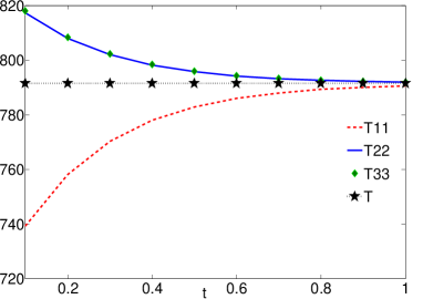
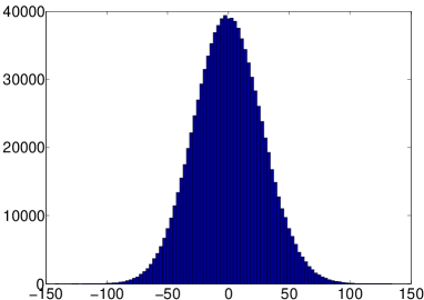
Figure 1: Left: time evolution of the diagonal components $T_{11},T_{22},T_{33}$ of the tensor $\Theta$ and of its trace $T$. Right: histogram of the first component of velocity at final time $t=1$.

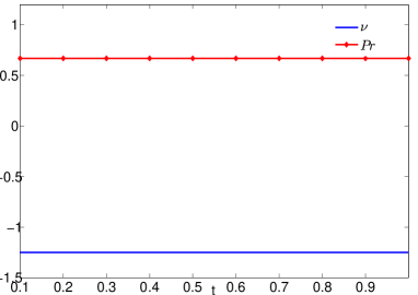
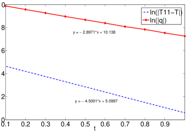
Figure 2: Left: time evolution of $\nu$ (defined by (35)) and $Pr$ (defined by (34)). Right: time history of $\log|T-T_{11}|$ and $\log|q|$.

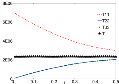
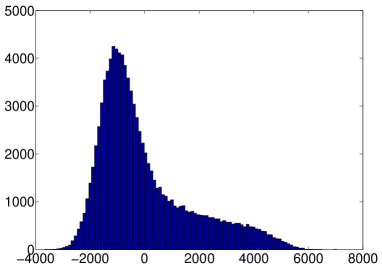
Figure 3: Left: time evolution of the diagonal components $T_{11},T_{22},T_{33}$ of the tensor $\Theta$ and of its trace $T$. Right: histogram of the first component of the velocity at time $t=0.5$.

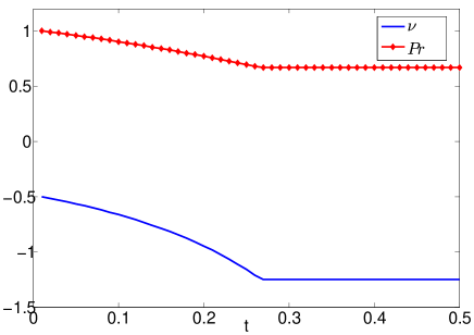
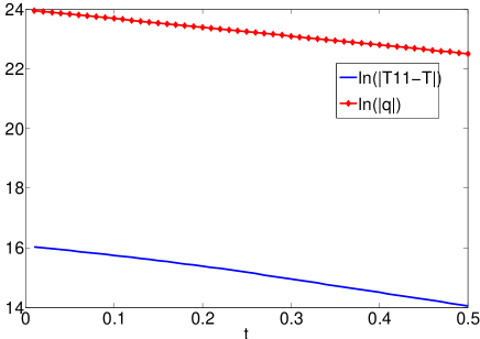
Figure 4: Left: $\nu$ and $Pr$ along time. Right: convergence of the logarithms of $|T-T_{11}|$ and $q$

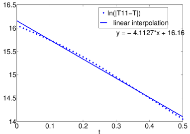
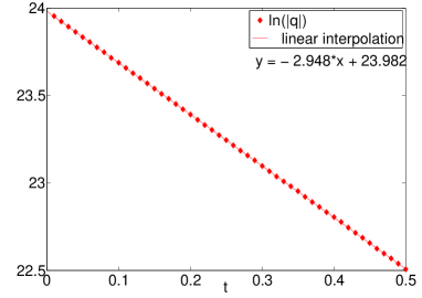
Figure 5: Left: comparison between the curve of the logarithm of $|T-T_{11}|$ ant its linear fitting. Right: comparison between the curve of the logarithm of $|q|$ ant its linear fitting.

References

- [1] P. Andriès, J.-F. Bourgat, P. Le Tallec, and B. Perthame. Numerical comparison between the Boltzmann and ES-BGK models for rarefied gases. Technical Report 3872, INRIA, 2000.
- [2] P. Andriès, P. Le Tallec, J.-F. Perlat, and B. Perthame. The Gaussian-BGK model of Boltzmann equation with small Prandtl number. Eur. J. Mech. B/Fluids, 2000.
- [3] C. Baranger, J. Claudel, N. Hérouard, and L. Mieussens. Locally refined discrete velocity grids for stationary rarefied flow simulations. Journal of Computational Physics, 257, Part A(0):572 – 593, 2014.
- [4] G.A. Bird. Molecular Gas Dynamics and the Direct Simulation of Gas Flows. Oxford Science Publications, 1994.
- [5] C. Cercignani. The Boltzmann Equation and Its Applications, volume 68. Springer-Verlag, Lectures Series in Mathematics, 1988.
- [6] S. Chen, K. Xu, C. Lee, and Q. Cai. A unified gas kinetic scheme with moving mesh and velocity space adaptation. Journal of Computational Physics, 231(20):6643 – 6664, 2012.
- [7] S. Chigullapalli and A. Alexeenko. Unsteady 3d rarefied flow solver based on boltzmann-esbgk model kinetic equations. In 41st AIAA Fluid Dynamics Conference and Exhibit. AIAA, June 27-30 2011. AIAA Paper 2011-3993.
- [8] D.H. Davis. Monte carlo calculation of molecular flow rates through a cylindrical elbow and pipes of other shapes. J. Appl. Phys., 31:1169–1176, 1960.
- [9] G. Dimarco and L. Pareschi. Numerical methods for kinetic equations. Acta Numerica, 23:369–520, 2014.
- [10] Hossein Gorji and Patrick Jenny. A Kinetic Model for Gas Mixtures Based on a Fokker-Planck Equation. Journal of Physics: Conference Series, 362(1):012042–, 2012.
- [11] M. Hossein Gorji and Patrick Jenny. A Fokker-Planck based kinetic model for diatomic rarefied gas flows. Physics of fluids, 25(6):062002–, June 2013.
- [12] M.H. Gorji, M. Torrilhon, and Patrick Jenny. Fokker–Planck model for computational studies of monatomic rarefied gas flows. Journal of fluid mechanics, 680:574–601, August 2011.
- [13] Patrick Jenny, Manuel Torrilhon, and Stefan Heinz. A solution algorithm for the fluid dynamic equations based on a stochastic model for molecular motion. Journal of computational physics, 229(4):1077–1098, 2010.
- [14] V.I. Kolobov, R.R. Arslanbekov, V.V. Aristov, A.A. Frolova, and S.A. Zabelok. Unified solver for rarefied and continuum flows with adaptive mesh and algorithm refinement. Journal of Computational Physics, 223(2):589 – 608, 2007.
- [15] Bernard Lapeyre, Étienne Pardoux, Rémi Sentis, and Société de mathématiques appliquées et industrielles (France) ). Méthodes de Monte-Carlo pour les équations de transport et de diffusion. Mathématiques et applications. Springer, Berlin, 1998. Cet ouvrage est une version remaniée des notes d’un cours présenté par les auteurs en préliminaire au 25e Congrès d’analyse numérique, les 22 et 23 mai 1993.
- [16] Z.-H. Li and H.-X. Zhang. Gas-kinetic numerical studies of three-dimensional complex flows on spacecraft re-entry. Journal of Computational Physics, 228(4):1116 – 1138, 2009.
- [17] L. Mieussens. A survey of deterministic solvers for rarefied flows. submitted, 2014.
- [18] G.A. Radtke, N. G. Hadjiconstantinou, and W. Wagner. Low-noise monte carlo simulation of the variable hard-sphere gas. Physics of Fluids, 23:030606, 2011.
- [19] V.A. Titarev. Efficient deterministic modelling of three-dimensional rarefied gas flows. Commun. Comput. Phys., 12(1):162–192, 2012.
- [20] L. Wu, J.M. Reese, and Y.H. Zhang. Oscillatory rarefied gas flow inside rectangular cavities. Journal of Fluid Mechanics, 748:350–367, 2014.