A randomized online quantile summary in $O(\frac{1}{\varepsilon}\log\frac{1}{\varepsilon})$ words

Abstract

A quantile summary is a data structure that approximates to $\varepsilon$-relative error the order statistics of a much larger underlying dataset.

In this paper we develop a randomized online quantile summary for the cash register data input model and comparison data domain model that uses $O(\frac{1}{\varepsilon}\log\frac{1}{\varepsilon})$ words of memory. This improves upon the previous best upper bound of $O(\frac{1}{\varepsilon}\log^{3/2}\frac{1}{\varepsilon})$ by Agarwal et. al. (PODS 2012). Further, by a lower bound of Hung and Ting (FAW 2010) no deterministic summary for the comparison model can outperform our randomized summary in terms of space complexity. Lastly, our summary has the nice property that $O(\frac{1}{\varepsilon}\log\frac{1}{\varepsilon})$ words suffice to ensure that the success probability is $1-e^{-\text{poly}(1/\varepsilon)}$.

1 Introduction

A quantile summary $S$ is a fundamental data structure that summarizes an underlying dataset $X$ of size $n$, in space much less than $n$. Given a query $\phi$, $S$ returns a sample $y$ of $X$ such that the rank of $y$ in $X$ is (probably) approximately $\phi n$. Quantile summaries are used in sensor networks to aggregate data in an energy-efficient manner and in database query optimizers to generate query execution plans.

Quantile summaries have been developed for a variety of different models and metrics. The data input model we consider is the standard online cash register streaming model, in which a new item is added to the dataset at each new timestep, and the total number of items is not known until the end. The data domain model we consider is the comparison model, in which stream items come from an arbitrary ordered domain (and specifically, not necessarily from the integers).

Formally, our quantile summary problem is defined over a totally ordered domain $\mathcal{D}$ and by an error parameter $\varepsilon\leq 1/2$. There is a dataset $X$ that is initially empty. Time occurs in discrete steps. In timestep $t$, stream item $x_{t}$ arrives and is then processed, and then any quantile queries $\phi$ in that step are received and processed. To be definite, we pick the first timestep to be $1$. We write $X_{t}$ or $X(t)$ for the $t$-item prefix stream $x_{1}\ldots x_{t}$ of $X$. The goal is to maintain at all times $t$ a summary $S_{t}$ of the dataset $X_{t}$ that, given any query $\phi$ in $(0,1]$, can return a sample $y=y(\phi)$ so that $|R(y,X_{t})-\phi t|\leq\varepsilon t$, where $R(a,Z)$ is the rank of item $a$ in set $Z$, defined as $|\{z\in Z:a\leq z\}|$. For randomized summaries, we only require that $\forall t\forall\phi,\;P(|R(y,X_{t})-\phi t|\leq\varepsilon t)\,\geq\,2/3$; that is, $y$’s rank is only probably close to $\phi t$, not definitely close. In fact, it will be easier to deal with the rank directly, so we define $\rho=\phi t$ and use that in what follows.

1.1 Previous work

The two most directly relevant pieces of prior work are randomized online quantile summaries for the cash register/comparison model. Aside from oblivious sampling algorithms (which require storing $\Omega(1/\varepsilon^{2})$ samples) we are unaware of any other randomized online quantile summaries that work in the comparison model.

The newer of the two is that of Agarwal, Cormode, Huang, Phillips, Wei, and Yi [1] [2]. Among other results, Agarwal et. al. develop a randomized online quantile summary for the cash register/comparison model that uses $O(\frac{1}{\varepsilon}\log^{3/2}\frac{1}{\varepsilon})$ words of memory. This summary has the nice property that any two such summaries can be combined to form a summary of the combined underlying dataset without loss of accuracy or increase in size.

The earlier such summary is that of Manku, Rajagopalan, and Lindsay [6], which uses $O(\frac{1}{\varepsilon}\log^{2}\frac{1}{\varepsilon})$ space. At a high level, their algorithm downsamples the input stream in a non-uniform way and feeds the downsampled stream into a deterministic summary, which periodically adjusts the downsampling rate.

We note here that our algorithm is inspired by the algorithm of Manku et. al. but has important differences. We defer a discussion of the similarities and differences to section 4 after the presentation of our algorithm in section 3.

For the comparison model, the best deterministic online summary to date is the (GK) summary of Greenwald and Khanna [3], which uses $O(\frac{1}{\varepsilon}\log\varepsilon n)$ space. This improved upon a deterministic (MRL) summary of Manku, Rajagopalan, and Lindsay [5] and a summary implied by Munro and Paterson [7], which use $O(\frac{1}{\varepsilon}\log^{2}\varepsilon n)$ space.

A more restrictive domain model than the comparison model is the bounded universe model, in which elements are drawn from the integers $\{1,\ldots,u\}$. For this model there is a deterministic online summary by Shrivastava, Buragohain, Agrawal, and Suri [8] that uses $O(\frac{\log u}{\varepsilon})$ space.

Not much exists in the way of lower bounds for this problem. There is a simple lower bound of $\Omega(1/\varepsilon)$ which intuitively comes from the fact that no one sample can satisfy more than $2\varepsilon n$ different rank queries. For the comparison model, Hung and Ting [4] developed a deterministic $\Omega(\frac{1}{\varepsilon}\log\frac{1}{\varepsilon})$ lower bound. Whether this bound can be extended to hold for our weaker probabilistic guarantee, and whether our algorithm can be modified to satisfy the stronger deterministic guarantee, are both open questions.

1.2 Our results

In the next section we describe a simple $O(\frac{1}{\varepsilon}\log\frac{1}{\varepsilon})$ streaming summary that is online except that it requires $n$ to be given up front and that it is unable to process queries until it has seen a constant fraction of the input stream. In section 3 we develop this simple summary into a fully online summary that can answer queries at any point in time. We close in section 4 by examining the similarities and differences between our summary and previous work and discuss a design approach for similar streaming problems.

2 A simple streaming summary

Before we describe our algorithm we must first describe its two main components in a bit more detail than was used in the introduction. The two components are Bernoulli sampling and the GK summary [3].

2.1 Bernoulli sampling

Bernoulli sampling downsamples a stream $X$ of size $n$ to a sample stream $S$ by choosing to include each next item into $S$ with independent probability $m/n$. (As stated this requires knowing the size of $X$ in advance.) At the end of processing $X$, the expected size of $S$ is $m$, and the expected rank of any sample $y$ in $S$ is $E(R(y,S))=\frac{m}{n}R(y,X)$. In fact, for any times $t\leq n$ and partial streams $X_{t}$ and $S_{t}$, where $S_{t}$ is the sample stream of $X_{t}$, we have $E(|S_{t}|)=mt/n$ and $E(R(y,S_{t}))=\frac{m}{n}R(y,X_{t})$. To generate an estimate for $R(y,X_{t})$ from $S_{t}$ we use $\hat{R}(y,X_{t})=\frac{n}{m}R(y,S_{t})$. The following theorem bounds the probability that $S$ is very large or that $\hat{R}(y,X_{t})$ is very far from $R(y,X_{t})$ (for any given time $t\geq n/64$, but not for all times $t=n/64\ldots n$ combined). The proof is folklore, a simple application of Chernoff bounds.

Theorem 2.1.

For all times $t\geq n/64$, $P(|S_{t}|>2tm/n)\,<\,\exp(-m/192)$.

Further, for all times $t\geq n/64$ and items $y$, $P(|\hat{R}(y,X_{t})-R(y,X_{t})|>\varepsilon t/8)\,<\,2\exp(-\varepsilon^{2}m/12288)$.

Proof.

For the first part, $P(|S_{t}|>2tm/n)\,<\,\exp(-tm/3n)\,<\,\exp(-m/192)$ (since $t\geq n/64$).

For the second part, $P(|\hat{R}(y,X_{t})-R(y,X_{t})|>\varepsilon t/8)$ is equal to $P(|R(y,S_{t})-E(R(y,S_{t}))|>\varepsilon tm/8n)$. The Chernoff bound is $P(|R(y,S_{t})-E(R(y,S_{t}))|>\delta E(R(y,S_{t})))\,<\,2\exp(-\min\{\delta,\delta^{2}\}E(R(y,S_{t}))/3)$. Here, $\delta=\varepsilon t/8R(y,S_{t})$, so $P<2\exp(-\varepsilon^{2}t^{2}m/192nE(R(y,S_{t})))\leq 2\exp(-\varepsilon^{2}m/12288)$. ∎

This means that, given any $1\leq\rho\leq t$, if we return the sample $y\in S_{t}$ with $R(y,S_{t})=\rho m/n$, then $R(y,X_{t})$ is likely to be close to $\rho$.

2.2 GK summary

The GK summary is a deterministic summary that can answer queries to relative error, over any portion of the received stream. If $G_{t}$ is the summary after inserting the first $t$ items $X_{t}$ from stream $X$ into $G$ then, given any $1\leq\rho\leq t$, $G_{t}$ can return a sample $y\in X_{t}$ so that $|R(y,X_{t})-\rho|\leq\varepsilon t/8$. Greenwald and Khanna guarantee in [3] that $G_{t}$ uses $O(\frac{1}{\varepsilon}\log(\varepsilon t))$ words. We call this the GK guarantee.

2.3 Our summary

We combine Bernoulli sampling with the GK summary by downsampling the input data stream $X$ to a sample stream $S$ and then feeding $S$ into a GK summary $G$. It looks like this:

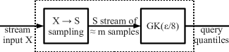
Figure 1: The big picture.

The key reason this gives us a small summary is that we never need to store $S$; each time we sample an item into $S$ we immediately feed it into $G$. Therefore, we only use as much space as $G(S(X_{t}))$ uses. In particular, as long as $m=O(\text{poly}(1/\varepsilon))$, we use only $O(\frac{1}{\varepsilon}\log\frac{1}{\varepsilon})$ words.

To answer a query $\rho$ for $X_{t}$ we ask $G_{t}$ the query $\rho m/n$ and return the resulting sample $y$. There is a slight issue in that $\rho m/n$ may be larger than $|S|$; but if the approximation guarantee holds for the largest item in $X_{t}$ then $\rho m/n<(t\!+\!\varepsilon t/8)m/n$, so using $\min\{\rho m/n,|S|\}$ instead will not cause more than $\varepsilon/8$ relative error in the approximation.

The probability that our sample stream $S_{t}$ is not too big (uses more than $2tm/n$ samples) is at least $1-\exp(-m/192)$. If this happens to be the case then the probability that all of its samples $y$ are good (have $|R(y,S_{t})-E(R(y,S_{t}))|\leq\varepsilon tm/8n$) is at least $1-4m\exp(-\varepsilon^{2}m/12288)$ by theorem 2.1 and the union bound. Choosing $m\geq\frac{300000\ln 1/\varepsilon}{\varepsilon^{2}}$ suffices to guarantee that both events occur with total probability at least $2/3$.

Further, if both $S_{t}$ events occur then the total error introduced by both $S_{t}$ and $G_{t}$ is at most $\varepsilon t/2$. Suppose that $G_{t}$ returns $y$ when given $\rho m/n$. This means that $|R(y,S_{t})-\rho m/n|\leq\varepsilon|S_{t}|\leq\varepsilon(2tm/n)/8$ by the GK guarantee. Since both events for $S_{t}$ occur, we also have $|R(y,S_{t})-\frac{m}{n}R(y,X_{t})|\leq\varepsilon tm/4n$ (and only $\varepsilon tm/8n$ in the case that we don’t truncate $\rho m/n$ to $|S|$). Thus, $|\frac{m}{n}R(y,X_{t})-\rho m/n|\leq\varepsilon tm/2n$. Equivalently, $|R(y,X_{t})-\rho|\leq\varepsilon t/2$.

2.4 Caveats

There are two serious issues with this summary. The first is that it requires us to know the value of $n$ in advance to perform the sampling. Also, as a byproduct of the sampling, we can only obtain approximation guarantees after we have seen at least $1/64$ (or at least some constant fraction) of the items. This means that while the algorithm is sufficient for approximating order statistics over streams stored on disk, more is needed to get it to work for online streaming applications, in which (1) the stream size $n$ is not known in advance, and (2) queries can be answered approximately at all times $t\leq n$ and not just when $t\geq n/64$.

Adapting the idea of our basic streaming summary to work online constitutes the next section and the bulk of our contribution. We start with a high-level overview of our online summary algorithm. In section 3.1 we formally define an initial version of our algorithm whose expected size at any given time is $O(\frac{1}{\varepsilon}\log\frac{1}{\varepsilon})$ words. In section 3.2 we show that our algorithm gurantees that $\forall n\forall\rho,\;P(|R(y,X_{n})-\rho|\leq\varepsilon n)\,\geq\,1-\exp(-1/\varepsilon)$. In section 3.3 we discuss the slight modifications necessary to get a deterministic $O(\frac{1}{\varepsilon}\log\frac{1}{\varepsilon})$ space complexity, and also perform a time complexity analysis.

3 An online summary

Our algorithm works in rows, which are illustrated in appendix A. Row $r$ is a summary of the first $2^{r}32m$ stream items. Since we don’t know how many items will actually be in the stream, we can’t start all of these rows running at the outset. Therefore, we start each row $r\geq 1$ once we have seen $1/64$ of its total items. However, since we can’t save these items for every row we start, we need to construct an approximation of this fraction of the stream, which we do by using the summary of the previous row, and join this approximating stream with the new items that arrive while the row is live. We then wait until the row has seen a full half of its items before we permit it to start answering queries; this dilutes the influence of approximating the $1/64$ of its input that we couldn’t store.

Operation within a row is very much like the operation of our fixed-$n$ streaming summary. We feed the joint approximate prefix + new item stream through a Bernoulli sampler to get a sample stream, which is then fed into a GK summary (which is stored). After row $r$ has seen half of its items, its GK summary becomes the one used to answer quantile queries. When row $r+1$ has seen $1/64$ of its total items, row $r$ generates an approximation of those items from its GK summary and feeds them as a stream into row $r+1$.

Row $0$ is slightly different in order to bootstrap the algorithm. There is no join step since there is no previous row to join. Also, row $0$ is active from the start. Lastly, we get rid of the sampling step so that we can answer queries over timesteps $1\ldots m/2$.

After the first $32m$ items, row $0$ is no longer needed, so we can clean up the space used by its GK summary. Similarly, after the first $2^{r}32m$ items, row $r$ is no longer needed. The upshot of this is that we never need storage for more than six rows at a time. Since each GK summary uses $O(\frac{1}{\varepsilon}\log\frac{1}{\varepsilon})$ words, the six live GK summaries use only a constant factor more.

Our error analysis, on the other hand, will require us to look back as many as $\Omega(\log 1/\varepsilon)$ rows to ensure our approximation guarantee. We stress that we will not need to actually store these $\Omega(\log 1/\varepsilon)$ rows for our guarantee to hold; we will only need that they didn’t have any bad events (as will be defined) when they were alive.

3.1 Algorithm description

Our algorithm works in rows. Each row $r$ has its own copy $G_{r}$ of the GK algorithm that approximates its input to $\varepsilon/8$ relative error. For each row $r$ we define several streams: $A_{r}$ is the prefix stream of row $r$, $B_{r}$ is its suffix stream, $R_{r}$ is its prefix stream replacement (generated by the previous row), $J_{r}$ is the joint stream $R_{r}$ followed by $B_{r}$, $S_{r}$ is its sample stream, and $Q_{r}$ is a one-time stream generated from $G_{r}$ by querying it with ranks $\rho_{1}\ldots\rho_{8/\varepsilon}$, where $\rho_{q}=q(\varepsilon/8)(m/64)$.

The prefix stream $A_{r}=X(2^{r-1}m)$ for row $r\geq 1$, importantly, is not directly received by row $r$. Instead, at the end of timestep $2^{r-1}m$, row $r\!-\!1$ generates $Q_{r-1}$ and duplicates each of those $8/\varepsilon$ items $2^{r-1}\varepsilon m/8$ times to get the replacement prefix $R_{r}$, which is then immediately fed into row $r$ before timestep $2^{r-1}m\!+\!1$ begins.

Each row can be live or not and active or not. Row $0$ is live in timesteps $1\ldots 32m$ and row $r\geq 1$ is live in timesteps $2^{r-1}m\!+\!1\ldots 2^{r}32m$. Live rows require space; once a row is no longer live we can free up the space it used. Row $0$ is active in timesteps $1\ldots 32m$ and row $r\geq 1$ is active in timesteps $2^{r}16m\!+\!1\ldots 2^{r}32m$. This definition means that exactly one row $r(t)$ is active in any given timestep $t$. Any queries that are asked in timestep $t$ are answered by $G_{r(t)}$. Given query $\rho$, we ask $G_{r(t)}$ for $\rho/2^{r(t)}32$ and return the result.

At each timestep $t$, when item $x_{t}$ arrives, it is fed as the next item in the suffix stream $B_{r}$ for each live row $r$. $B_{r}$ joined with $R_{r}$ defines the joined input stream $J_{r}$. For $r\geq 1$, $J_{r}$ is downsampled to the sample stream $S_{r}$ by sampling each item independently with probability $1/2^{r}32$. For row $0$, no downsampling is performed, so $S_{0}=J_{0}$. Lastly, $S_{r}$ is fed into $G_{r}$.

Appendix A shows the operation of and the communication between the first six rows. Solid arrows indicate continuous streams and dashed arrows indicate one-time messages. Appendix B is a pseudocode listing of the algorithm.

3.2 Error analysis

Define $C_{r}=x(2^{r}32m\!+\!1),x(2^{r}32m\!+\!2),\ldots$ and $Y_{r}$ to be $R_{r}$ followed by $B_{r}$ and then $C_{r}$. That is, $Y_{r}$ is just the continuation of $J_{r}$ for the entire length of the input stream.

Fix some time $t$. All of our claims will be relative to time $t$; that is, if we write $S_{r}$ we mean $S_{r}(t)$. Our error analysis proceeds as follows. We start by proving that $R(y,Y_{r})$ is a good approximation of $R(y,Y_{r-1})$ when certain conditions hold for $S_{r-1}$. By induction, this means that $R(y,Y_{r})$ is a good approximation of $R(y,X\!=\!Y_{0})$ when the conditions hold for all of $S_{0}\ldots S_{r-1}$, and actually it’s enough for the conditions to hold for just $S_{r-\log 1/\varepsilon}\ldots S_{r-1}$ to get a good approximation. Having proven this claim, we then prove that the result $y=y(\rho)$ of a query to our summary has $R(y,X)$ close to $\rho$. Lastly, we show that $m=O(\text{poly}(1/\varepsilon))$ suffices to ensure that the conditions hold for $S_{r-\log 1/\varepsilon}\ldots S_{r-1}$ with very high probability ($1-e^{-1/\varepsilon}$).

Lemma 3.1.

Let $\alpha_{r}$ be the event that $|S_{r}|>2m$ and let $\beta_{r}$ be the event that any of the first $\leq 2m$ samples $z$ in $S_{r}$ has $|2^{r}32R(z,S_{r})-R(z,Y_{r})|>\varepsilon t/8$. Say that $S_{r}$ is good if neither $\alpha_{r}$ nor $\beta_{r}$ occur (or if $r=0$).

For all $r\geq 1$ such that $t\geq t_{r}=2^{r-1}m$, and for all items $y$, if $S_{r-1}$ is good then $|R(y,Y_{r})-R(y,Y_{r-1})|\leq 2^{r}\varepsilon m$.

Proof.

At the end of time $t_{r}$ we have $Y_{r}(t_{r})=R_{r}(t_{r})$, which is each item $y(\rho_{q})$ in $Q_{r-1}$ duplicated $\varepsilon t_{r}/8$ times. If $S_{r-1}(t_{r})$ is good then by theorem 2.1 and the GK guarantee we have that $|R(y(\rho_{q}),Y_{r-1}(t_{r}))-2^{r-1}32\rho_{q}|\leq\varepsilon t_{r}/2$.

Fix $q$ so that $y(\rho_{q})\leq y<y(\rho_{q+1})$, where $y(\rho_{0})$ and $y(\rho_{1\!+\!8/\varepsilon})$ are defined to be $\min X_{t}$ and $\sup\mathcal{D}$ for completeness. Fixing $q$ this way implies that $R(y,Y_{r}(t_{r}))=2^{r-1}32\rho_{q}$. By the above bound on $R(y(\rho_{q}),Y_{r-1}(t_{r}))$ we also have that $2^{r-1}32\rho_{q}-\varepsilon t_{r}/2\leq R(y,Y_{r-1}(t_{r}))<2^{r-1}32\rho_{q+1}+\varepsilon t_{r}/2$.

Putting these two bounds together, and recalling that $\rho_{q}=q\varepsilon m/512$, we find that $|R(y,Y_{r}(t_{r}))-R(y,Y_{r-1}(t_{r}))|\leq 2^{r}\varepsilon m$. For each time $t$ after $t_{r}$, the new item $x_{t}$ changes the rank of $y$ in both streams $Y_{r}$ and $Y_{r-1}$ by the same additive offset, so $|R(y,Y_{r})-R(y,Y_{r-1})|=|R(y,Y_{r}(t_{r}))-R(y,Y_{r-1}(t_{r}))|\leq 2^{r}\varepsilon m$. ∎

By applying this lemma inductively we can bound the difference between $Y_{r}$ and $X=Y_{0}$:

Corollary 3.2.

For all $r\geq 1$ such that $t\geq t_{r}=2^{r-1}m$, if all of $S_{0}(t_{1}),S_{1}(t_{2}),\ldots,$ $S_{r-1}(t_{r})$ are good, then $|R(y,Y_{r})-R(y,X)|\leq 2^{r+1}\varepsilon m$.

To ensure that all of these $S_{i}$ are good would require $m$ to grow with $n$, which would be bad. Happily, it is enough to require only the last $\log_{2}1/\varepsilon$ sample summaries to be good, since the other items we disregard constitute only a small fraction of the total stream.

Corollary 3.3.

Let $d=\log_{2}1/\varepsilon$. For all $r\geq 1$ such that $t\geq t_{r}=2^{r-1}m$, if all of $S_{r-1}(t_{r}),\ldots,S_{r-d}(t_{r-d+1})$ are good, then $|R(y,Y_{r})-R(y,X)|\leq 2^{r+2}\varepsilon m$.

Proof.

By lemma 3.1 we have $|R(y,Y_{r})-R(y,Y_{r-d})|\leq 2^{r+1}\varepsilon m$. At time $t\geq t_{r-d}$, $Y_{r-d}$ and $X$ share all except possibly the first $2^{(r-d)-1}m=2^{r-1}m/2^{d}=2^{r-1}\varepsilon m$ items. Thus

$$|R(y,Y_{r})-R(y,X)| \leq|R(y,Y_{r})-R(y,Y_{r-d})|+|R(y,Y_{r-d})-R(y,X)|$$

$$\leq 2^{r+1}\varepsilon m+2^{r}\varepsilon m$$

We now prove that the if the last several sample streams were good then querying our summary will give us a good result.

Lemma 3.4.

Let $d=\log_{2}\frac{1}{\varepsilon}$ and $r=r(t)$. If all $S_{r}(t),S_{r-1}(t_{r}),\ldots,S_{r-d}(t_{r-d+1})$ are good, then querying our summary with rank $\rho$ (= querying the active GK summary $G_{r}$ with $\rho/2^{r}32$) returns $y=y(\rho)$ such that $|R(y,X)-\rho|\leq\varepsilon t$.

Proof.

By corollary 3.3 we have $|R(y,Y_{r})-R(y,X)|\leq 2^{r+2}\varepsilon m\leq\varepsilon t/2$. By theorem 2.1 and the GK guarantee, $|R(y,Y_{r})-\rho|\leq\varepsilon t/2$. ∎

Lastly, we prove that $m=O(\text{poly}(1/\varepsilon))$ suffices to ensure that all of $S_{r}(t),$ $S_{r-1}(t_{r}),\ldots,S_{r-d}(t_{r-d+1})$ are good with probability at least $1-e^{-1/\varepsilon}$.

Lemma 3.5.

Let $d=\log_{2}1/\varepsilon$ and $r=r(t)$. If $m\geq\frac{400000\ln 1/\varepsilon}{\varepsilon^{2}}$ then all of $S_{r}(t),S_{r-1}(t_{r}),\ldots,S_{r-d}(t_{r-d+1})$ are good with probability at least $1-e^{-1/\varepsilon}$.

Proof.

There are at most $1\!+\!\log_{2}1/\varepsilon\leq 4\ln 1/\varepsilon$ of these summary streams total. Theorem 2.1 and the union bound give us $P(\text{no $\alpha_{r}$ occurs})\leq 4\ln\frac{1}{\varepsilon}\exp(-m/192)$ and $P(\text{no $\beta_{r}$ occurs})\leq 16m\ln\frac{1}{\varepsilon}\exp(-\varepsilon^{2}m/12288)$.

Together, $P=P(\text{some $S_{r}$ is not good})\leq 20m\ln\frac{1}{\varepsilon}\exp(-\varepsilon^{2}m/12288)$. It suffices to choose $m\geq\frac{400000\ln 1/\varepsilon}{\varepsilon^{2}}$ to obtain $P\leq e^{-1/\varepsilon}$. ∎

3.3 Space and time complexity

A minor issue with the algorithm is that, as written in section 3.1, we do not actually have a bound on the worst-case space complexity of the algorithm; we only have a bound on the space needed at any given point in time. This issue is due to the fact that there are low probability events in which $|S_{r}|$ can get arbitrarily large and the fact that over $n$ items there are a total of $\Omega(\log n)$ sample streams. The space complexity of the algorithm is $O(\max|S_{r}|)$, and to bound this value with constant probability using the Chernoff bound appears to require that $\max|S_{r}|=\Omega(\log\log n)$, which is too big.

Fortunately, fixing this problem is simple. Instead of feeding every sample of $S_{r}$ into the GK summary $G_{r}$, we only feed each next sample if $G_{r}$ has seen $<2m$ samples so far. That is, we deterministically restrict $G_{r}$ to receiving only $2m$ samples. Lemmas 3.1 through 3.4 condition on the goodness of the sample streams $S_{r}$, which ensures that the $G_{r}$ receive at most $2m$ samples each, and the claim of lemma 3.5 is independent of the operation of $G_{r}$. Therefore, by restricting each $G_{r}$ to receive at most $2m$ inputs we can ensure that the space complexity is deterministically $O(\frac{1}{\varepsilon}\log\frac{1}{\varepsilon})$ without breaking our error guarantees.

From a practical perspective, the assumption in the streaming setting is that new items arrive over the input stream $X$ at a high rate, so both the worst-case per-item processing time as well as the amortized time to process $n$ items are important. For our per-item time complexity, the limiting factor is the duplication step that occurs at the end of each time $t_{r}=2^{r-1}m$, which makes the worst-case per-item processing time as large as $\Omega(n)$. Instead, at time $t_{r}$ we could generate $Q_{r-1}$ and store it in $O(1/\varepsilon)$ words, and then on each arrival $t=2^{r-1}m\!+\!1\ldots 2^{r}m$ we could insert both $x_{t}$ and also the next item in $R_{r}$. By the time $t_{r+1}=2t_{r}$ that we generate $Q_{r}$, all items in $R_{r}$ will have been inserted into $J_{r}$. Thus the worst-case per-item time complexity is $O(\frac{1}{\varepsilon}T_{\text{GK}}^{\text{max}})$, where $T_{\text{GK}}^{\text{max}}$ is the worst-case per-item time to query or insert into one of our GK summaries. Over $2^{r}32m$ items there are at most $2m$ insertions into any one GK summary, so the amortized time over $n$ items in either case is $O(\frac{m\log n/32m}{n}T_{\text{GK}})$, where $T_{\text{GK}}$ is the amortized per-item time to query or insert into one of our GK summaries.

The pseudocode listing in appendix B includes the changes of this section.

4 Discussion

Our starting point is a very natural idea of Manku et. al. [6] that due to subtle technical difficulties saw no further application to the quantiles problem for sixteen years. This key idea is to downsample the input stream and feed the resulting sample stream into a deterministic summary data structure (compare our figure 1 with figure 1 on page 254 of [6]). At a very high level, we are simply replacing their deterministic $O(\frac{1}{\varepsilon}\log^{2}\varepsilon n)$ MRL summary [5] with the deterministic $O(\frac{1}{\varepsilon}\log\varepsilon n)$ GK summary [3]. However, as evidenced by the fact that fourteen years after the GK summary was published the state of the art was the randomized $O(\frac{1}{\varepsilon}\log^{3/2}\frac{1}{\varepsilon})$ summary of Agarwal et. al. [1] [2], adapting this idea to the GK summary without superconstant overhead is nontrivial.

Our implementation of this idea is conceptually different from the implementation of Manku et. al. in two respects. First, we use the GK algorithm strictly as a black box, whereas Manku et. al. peek into the internals of their MRL algorithm, using its algorithm-specific interface (New, Collapse, Output) rather than the more generic interface (Insert, Query). At an equivalent level, dealing with the GK algorithm is already unpleasant. Using the generic interface, our implementation could just as easily replace the GK boxes in the diagram in appendix A with MRL boxes; or, for the bounded universe model, with boxes running the q-digest summary of Shrivastava et. al. [8].

The second respect in which our algorithm differs critically from that of Manku et. al. is that we operate on streams rather than on stream items. We use this approach in our proof strategy too; the key step in our error analysis, lemma 3.1, is a statement about (what to us are) static objects, so we can trade out the complexity of dealing with time-varying data structures for a simple induction.

The approach we developed to reduce a deterministic summary to a randomized summary was:

For a fixed $n$, downsample the input stream, feed the resulting sample stream into the deterministic summary, and prove a probabilistic bound.

Run an infinite number of copies of step 1, for exponentially growing values of $n$.

Replace a constant fraction prefix of each copy with an approximation generated by the previous copy, and prove using step 1 that this approximation probably doesn’t cause too much error.

Use step 3 inductively to prove a probabilistic bound for the entire stream. We believe (albeit on the basis of this problem and our algorithm alone) that developing streaming algorithms that operate on streams rather than on stream items is likely to be a useful design approach for many problems.

Appendix A Diagram for online algorithm

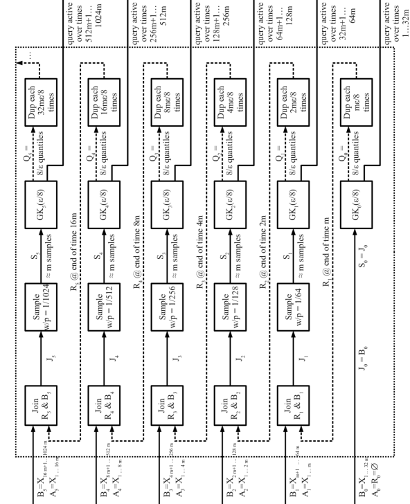
Figure 2: Each row $r$ has its own copy $G_{r}$ of the GK algorithm that approximates its input to $\varepsilon/8$ relative error. $A_{r}$ is the prefix stream of row $r$, $B_{r}$ is its suffix stream, $R_{r}$ is its prefix stream replacement (generated by the previous row), $J_{r}$ is the joint stream $R_{r}$ followed by $B_{r}$, $S_{r}$ is its sample stream, and $Q_{r}$ is a one-time stream generated from $G_{r}$ at time $2^{r}m$ to get the replacement prefix $R_{r+1}$.

Appendix B Pseudocode for online algorithm

The differences in the algorithms of sections 3.1 and 3.3 are marked.

Initially, allocate space for $G_{0}$. Mark row $0$ as live and active.

for $t=1,2,\ldots$ do

      foreach live row $r\geq 0$ do

           with probability $1/2^{r}32$ do

                if section 3.1 then

                     Insert $x_{t}$ into $G_{r}$.

                    

                     else if section 3.3 then

                          Insert $x_{t}$ into $G_{r}$ if $G_{r}$ has seen $<2m$ insertions.

                          if $r\geq 1$ and $2^{r-1}m<t\leq 2^{r}m$ and $G_{r}$ has seen $<2m$ insertions then

                               with probability $1/2^{r}32$ do

                                    Also insert item $t\!-\!2^{r-1}m$ of $R_{r}$ into $G_{r}$.

                                   

                                   

                                   

                                   

                                   

                                    if $t=2^{r-1}m$ for some $r\geq 1$ then

                                         Allocate space for $G_{r}$. Mark row $r$ as live.

                                         if section 3.1 then

                                              Query $G_{r-1}$ with $\rho_{1}\ldots\rho_{8/\varepsilon}$ to get $y_{1}\ldots y_{8/\varepsilon}$.

                                              for $q=1\ldots 8/\varepsilon$ do

                                                   for $1\ldots 2^{r-1}\varepsilon m/8$ do

                                                        with probability $1/2^{r}32$ do

                                                             Insert $y_{q}$ into $G_{r}$.

                                                            

                                                            

                                                            

                                                            

                                                             else if section 3.3 then

                                                                  Store $Q_{r-1}$, to implicitly define $R_{r}$.

                                                                 

                                                                 

                                                                  if $t=2^{r}16m$ for some $r\geq 1$ then

                                                                       Mark row $r$ as active. Unmark row $r\!-\!1$ as active.

                                                                      

                                                                       if $t=2^{r}32m$ for some $r\geq 0$ then

                                                                            Unmark row $r$ as live. Free space for $G_{r}$.

                                                                           

                                                                           

                                                                            on query $\rho$ do

                                                                                 Let $r(t)$ be the active row.

                                                                                 Query $G_{r(t)}$ for rank $\rho/2^{r(t)}32$. Return the result.

                                                                                

Algorithm 1 Procedural listing of the algorithm.

References

- [1] Pankaj K. Agarwal, Graham Cormode, Zengfeng Huang, Jeff Phillips, Zhewei Wei, and Ke Yi. Mergeable summaries. In Proceedings of the 31st Symposium on Principles of Database Systems, PODS ’12, pages 23–34, New York, NY, USA, 2012. ACM.
- [2] Pankaj K Agarwal, Graham Cormode, Zengfeng Huang, Jeff M Phillips, Zhewei Wei, and Ke Yi. Mergeable summaries. ACM Transactions on Database Systems (TODS), 38(4):26, 2013.
- [3] Michael Greenwald and Sanjeev Khanna. Space-efficient online computation of quantile summaries. In ACM SIGMOD Record, volume 30, pages 58–66. ACM, 2001.
- [4] Regant YS Hung and Hingfung F Ting. An omega ( frac 1 varepsilon log frac 1 varepsilon) space lower bound for finding -approximate quantiles in a data stream. In Frontiers in Algorithmics, pages 89–100. Springer, 2010.
- [5] Gurmeet Singh Manku, Sridhar Rajagopalan, and Bruce G Lindsay. Approximate medians and other quantiles in one pass and with limited memory. In ACM SIGMOD Record, volume 27, pages 426–435. ACM, 1998.
- [6] Gurmeet Singh Manku, Sridhar Rajagopalan, and Bruce G Lindsay. Random sampling techniques for space efficient online computation of order statistics of large datasets. In ACM SIGMOD Record, volume 28, pages 251–262. ACM, 1999.
- [7] J. I. Munro and M. S. Paterson. Selection and sorting with limited storage. In Proceedings of the 19th Annual Symposium on Foundations of Computer Science, SFCS ’78, pages 253–258, Washington, DC, USA, 1978. IEEE Computer Society.
- [8] Nisheeth Shrivastava, Chiranjeeb Buragohain, Divyakant Agrawal, and Subhash Suri. Medians and beyond: new aggregation techniques for sensor networks. In Proceedings of the 2nd international conference on Embedded networked sensor systems, pages 239–249. ACM, 2004.