Van der Waals interactions between excited atoms in generic environments

Abstract

We consider the the van der Waals force involving excited atoms in general environments, constituted by magnetodielectric bodies. We develop a dynamical approach studying the dynamics of the atoms and the field, mutually coupled. When only one atom is excited, our dynamical theory suggests that for large distances the van der Waals force acting on the ground-state atom is monotonic, while the force acting in the excited atom is spatially oscillating. We show how this latter force can be related to the known oscillating Casimir–Polder force on an excited atom near a (ground-state) body. Our force also reveals a population-induced dynamics: for times much larger that the atomic lifetime the atoms will decay to their ground-states leading to the van der Waals interaction between ground-state atoms.

I Introduction

Casimir and van der Waals (vdW) forces are interactions between neutral macroscopic bodies or atoms arising from the quantum fluctuations of both the electromagnetic field and the atomic charges Casimir48 ; CasimirPolder48 . They are responsible for many characteristic phenomena in physics, chemistry and biology: the deviation from ideal-gas behaviour in non-polar gases kihara , latent heat of liquids, capillary attraction, physical absorption, and cell adhesion nir . Dispersion interactions have even played an important role during the early stages of planet formation pater , and they are also supposed to have a fundamental role in selective long-distance biomolecular recognition Preto . Due to their strong distance-dependence, they become more and more important on the ever-decreasing scales of nanotechnology, where they lead to the unwanted stiction of small mobile components Serry . In a series of ground-breaking experiments, the vdW force between an excited barium ion and a mirror have been measured to high precision wilson ; bushev . Such experiments show an oscillating dependence of the vdW force on the ion.

We will focus on the vdW force between two atoms, in excited states $\left|n\right\rangle$ and $\left|l\right\rangle$. The interaction in this case is different from the interaction between two ground-state atoms due to the possible exchange of a real photon between the atoms. In the well-understood non-retarded regime, that is, for distances $r$ much smaller than the wavelength of atomic electronic transitions, one finds power3 ; Buhmann

$$\textbf{F}_{\text{nr}}\left(r\right)=-\frac{\textbf{e}_{r}}{4\pi^{2}\varepsilon_{0}^{2}r^{7}}\sum\limits_{k,p}\frac{|\textbf{d}_{nk}^{A}|^{2}|\textbf{d}_{pl}^{B}|^{2}}{E_{k}^{A}-E_{n}^{A}+E_{p}^{B}-E_{l}^{B}}$$ (1)

where, $\textbf{e}_{r}=\textbf{r}/r$, $\mathbf{d}_{nm}^{A}$ are the matrix-elements of the dipole operator and $E_{k}$ the energy relative to the state $\left|k\right\rangle$. For downward transitions, $E_{k}^{A}-E_{n}^{A}+E_{p}^{B}-E_{l}^{B}$ can be negative and the resulting energy positive, yielding a repulsive interaction. Hence non-equilibrium situations can provide repulsive vdW interactions.

The interaction at larger separations has been object of controversies. In a first group of works, it was predicted that the magnitude of the retarded potential oscillates as a function of interatomic distance Gomberoff ; McLone ; Philpott . In a later group of publications it was claimed that the retarded potential is non-oscillatory and proportional to $1/r^{2}$ power ; power2 ; power3 ; sherk . The conflicting results are due to subtle differences in treating divergent energy denominators in the photon propagators: the poles in the real axis can be avoided using the principal value prescription or adding infinitesimal factors in the energy denominators and this leads to different results. Both procedures are mathematically correct, but they yield different physical results: a spatially oscillatory behaviour of the interaction in the first case and a monotonically decreasing behaviour in the second.

A group of recent works have used dynamical approaches to address the problem. By an appropriate time-averaging procedure manuel or in the limit of vanishing atomic line widths berman , a third result, for the vdW interaction on the excited atom, was found that oscillates in magnitude and sign. Note that an earlier approach based on time-dependent perturbation theory yields a non-oscillatory result for the force on the ground-state atom that is however valid only for times shorter than the lifetime of the excited state rizzuto . Similar considerations about timescales hold for the diagrammatic non-equilibrium description used in Ref. Haakh .

A very recent work claims that both results, the monotonic and the oscillating, are valid, but they describe different physical processes milonni3 : the oscillating result is related to a coherent exchange of excitation between the atoms, while the monotonic result is associated to a fast loss of excitation acquired from the initially excited atom. Another recent work finds that both forces can simultaneously arise in a single set-up: the vdW interaction on the excited atom oscillates, in agreement with manuel ; berman ; milonni3 , but the vdW force acting on the ground-state atom is monotonic manuel2 . This result would imply an apparent violation of the action–reaction principle in excited systems in free space. However, it was shown that the momentum balance is restored when taking the photon emitted by the excited atom into account manuel3 . This emission being asymmetric due to the presence of the ground-state atom, the emitted photon carries some average momentum, so that the difference between forces on the excited vs ground-state atoms can be interpreted as a photon recoil force. The situation is somewhat similar to the lateral Casimir–Polder force on an atom near a nanofibre, which is also associated with asymmetric emission Scheel15 .

In this paper, we study the van der Waals interaction involving excited atoms by means of a dynamical approach on the basis of the Markov approximation. We show that the damped internal atomic dynamics uniquely determines the oscillatory or monotonic behavior of the retarded interaction for excited atoms. In our dynamical model, the poles in the real axis are automatically shifted to the upper or lower part of the complex plane, and no ad hoc choice for the imaginary shifts in the denominators is required. We will show that, when one atom is excited, the vdW force acting on the ground-state atom is monotonic and the vdW interaction of the excited atom is oscillating, in agreement with the most recent results in literature milonni3 ; manuel2 ; manuel3 ; safari . Our dynamical approach is an alternative to the time-dependent perturbation theory manuel2 , where the behaviour of the force is determined via a time average over rapid oscillations on time scales of the order of atomic transition frequencies. Instead, our model allows us to study the decay-induced dynamics on larger time scales of the order of the excited-state lifetimes. It reveals that the force is governed by population-induced dynamics on these scales, where for times much larger than the lifetime of the intial atomic state the vdW force converges to that between ground-state atoms. In addition, we are able to account for a general environment for the two atoms, via the classical Green tensor.

The article is organised as follows. In Sect. II, we present the basic formalism describing the coupled atom–field dynamics. It is used in Sect. III for calculating the force between two atoms in arbitrary excited initial states. In Sect. IV, we make the connection of our result with the Casimir–Polder force between an excited atom and a body of arbitrary shape. Some conclusions are given in Sect.  V, while in the Appendices, we present some of the more cumbersome details of our general approach and our calculation.

II Atom–field dynamics

We consider the mutually coupled evolution of two atoms and the medium-assisted field. The field is prepared at zero temperature, and the atoms in generic internal states. The dynamics of the atoms can be described with time-dependent flip operators, defined by $\hat{A}_{mn}=\left|m^{A}\right\rangle\left\langle n^{A}\right|$, where $\left|n^{A}\right\rangle$ is an energy eigenstate, and similarly $\hat{B}_{pq}=\left|p^{B}\right\rangle\left\langle q^{B}\right|$.

In order to evaluate the force between the two atoms we must first solve the atom-field dynamics to obtain the flip operators and the field operators in the Heisenberg picture. The total Hamiltonian is the sum of three terms, the atomic and the field Hamiltonian and the interaction term in the multipolar coupling scheme within dipole approximation:

$$\hat{H}= \hat{H}_{A}+\hat{H}_{F}+\hat{H}_{AF}$$

$$\hat{H}_{A}= \sum\limits_{n}E_{n}^{A}\hat{A}_{nn}+\sum\limits_{n}E_{n}^{B}\hat{B}_{nn}$$

$$\hat{H}_{F}= \sum\limits_{\lambda=e,m}\int\mathrm{d}^{3}r\int\limits_{0}^{\infty}\mathrm{d}\omega\hbar\omega\mathbf{\hat{f}}_{\lambda}^{\dagger}\left(\mathbf{r},\omega\right)\cdot\mathbf{\hat{f}}_{\lambda}\left(\mathbf{r},\omega\right)$$

$$\hat{H}_{AF}= -\mathbf{\hat{d}}^{A}\cdot\mathbf{\hat{E}}\left(\mathbf{r}_{A}\right)-\mathbf{\hat{d}}^{B}\cdot\mathbf{\hat{E}}\left(\mathbf{r}_{B}\right)$$ (2)

where $\mathbf{\hat{f}}_{\lambda}\left(\mathbf{r},\omega\right)$ is the annihilation operator for the elementary electric and magnetic excitations of the system Buhmann-Welsch .

Since the evolution of the whole system is unitary the commutator between two electric fields coincides with the commutator between free fields Buhmann2 ; knoll

$$\big{[}\mathbf{\hat{E}}\left(\mathbf{r},\omega\right),\mathbf{\hat{E}}^{\dagger}\left(\mathbf{r}^{\prime},\omega^{\prime}\right)\big{]}=\frac{\hbar\mu_{0}}{\pi}\textup{Im}\mbox{{{{G}}}}\left(\mathbf{r},\mathbf{r^{\prime}},\omega\right)\omega^{2}\delta\left(\omega-\omega^{\prime}\right)$$ (3)

where G is the Green’s tensor of the electromagnetic field and $\mathbf{\hat{E}}\left(\mathbf{r},\omega\right)$ is the Fourier component of the electric field $\mathbf{\hat{E}}\left(\mathbf{r}\right)=\int_{0}^{\infty}\text{d}\omega\mathbf{\hat{E}}\left(\mathbf{r},\omega\right)+\textup{h.c.}$, Heisenberg equations for the coupled atom–field dynamics read

$$\partial_{t}\hat{A}_{mn}=\mathrm{i}\omega_{mn}^{A}\hat{A}_{mn}+\frac{\mathrm{i}}{\hbar}\mathbf{\hat{K}}_{mn}^{A}\cdot\mathbf{\hat{E}}\left(\mathbf{r}_{A}\right)$$

$$\partial_{t}\mathbf{\hat{E}}\left(\mathbf{r},\omega\right)=-\mathrm{i}\omega\mathbf{\hat{E}}\left(\mathbf{r},\omega\right)$$

$$+\frac{\mathrm{i}\mu_{0}}{\pi}\omega^{2}\left[\textup{Im}\mbox{{{{G}}}}\left(\mathbf{r},\mathbf{r}_{A},\omega\right)\cdot\mathbf{\hat{d}}^{A}+\textup{Im}\mbox{{{{G}}}}\left(\mathbf{r},\mathbf{r}_{B},\omega\right)\cdot\mathbf{\hat{d}}^{B}\right]$$ (4)

where $\mathbf{\hat{K}}_{mn}^{A}=\left[\hat{A}_{mn},\mathbf{\hat{d}}^{A}\right]$.

The electric field at the position of atom A consists of two terms: the radiation reaction and the field due to the other atom B. As shown in the literature ackerhalt ; Buhmann2 , the radiation reaction field gives rise to frequency shifts and spontaneous decay for atom A, see Figs. 1(a) and (b). We thus renormalize the field by splitting off the radiation reaction

$$\left\langle\partial_{t}\hat{A}_{mn}\right\rangle=\left[\mathrm{i}\tilde{\omega}_{mn}^{A}-\left(\Gamma_{n}^{A}+\Gamma_{m}^{A}\right)/2\right]\left\langle\hat{A}_{mn}\right\rangle\\ +\frac{\mathrm{i}}{\hbar}\left\langle\mathbf{\hat{K}}_{mn}^{A}\cdot\mathbf{\hat{E}}_{\not}{A}\left(\mathbf{r}_{A},t\right)\right\rangle$$ (5)

where $m\neq n$ and the expectation value $\langle\ldots\rangle$ is taken over atomic state and the field thermal state. $\mathbf{\hat{E}}_{\not}{A}\left(\mathbf{r}_{A},t\right)$ is the sum of the free electric field and the source field of the atom B, $\tilde{\omega}_{mn}^{A}$ the (second-order) Lamb-shifted atomic frequencies and $\Gamma_{n}^{A}$ the decay rates.

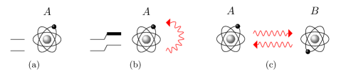
Figure 1: Case a) is the zero order approximation: free field and free atom. Case b) is the next order approximation: the Lamb shift of an atom due to the emission and re-absorption of a photon. Case c) is the dispersion interaction between two atoms due to the exchange of two photons.

III Van der Waals interaction between two excited atoms

We consider two atoms $A$ and $B$ that are initially prepared in excited energy eigenstates $\left|i_{A}\right\rangle$, $\left|i_{B}\right\rangle$ of the free atomic Hamiltonian ($p_{n}^{A}(0)=\delta_{ni_{A}},p_{l}^{B}(0)=\delta_{li_{B}}$). These initial states are not eigenstates of the total Hamiltonian and thus the atomic states evolve in time yielding a time-dependent vdW force (population-induced dynamics). As time progresses, the lower lying levels $n\leqslant i_{A}$,$l\leqslant i_{B}$ will become populated.

To find the vdW force between on, say, atom $A$, we calculate the Lorentz force in electric-dipole approximation acting on $A$ which is due to the field $\mathbf{E}_{\not}{A}\left(\mathbf{r}_{A},t\right)$ emitted by the other atom B:

$$\mathbf{F}_{A}(\mathbf{r}_{A},\mathbf{r}_{B},t)=\nabla_{A}\big{\langle}\mathbf{\hat{d}}^{A}\cdot\mathbf{\hat{E}}_{\not}{A}\left(\mathbf{r}_{A},t\right)\big{\rangle},$$ (6)

where expectation value is taken over atomic and field states.

For weak atom–field coupling, corresponding in an expansion of the Hamiltonian in powers of the coupling strengths d, we can apply the Markov approximation to find (see Appendix):

$$\textbf{F}_{A}\left(\mathbf{r}_{A},\mathbf{r}_{B},t\right)=\frac{\mu_{0}^{2}}{2\pi^{2}\hbar}\sum\limits_{n\leqslant i_{A}}\sum\limits_{l\leqslant i_{B}}p_{n}^{A}(t)p_{l}^{B}(t)\sum\limits_{k,p}\\ \times\int\limits_{0}^{\infty}\mathrm{d}\omega\int\limits_{0}^{\infty}\mathrm{d}\omega^{\prime}\omega^{2}\omega^{\prime 2}\nabla_{A}\left\{\mathbf{d}_{nk}^{A}\cdot\text{Im}\mbox{{{{G}}}}\left(\mathbf{r}_{A},\mathbf{r}_{B},\omega\right)\right.\cdot\mathbf{d}_{pl}^{B}\\ \left.\times\mathbf{d}_{lp}^{B}\cdot\text{Im}\mbox{{{{G}}}}\left(\mathbf{r}_{B},\mathbf{r}_{A},\omega^{\prime}\right)\cdot\mathbf{d}_{kn}^{A}\right\}\sum\limits_{i=1}^{16}\frac{1}{D_{i}}+\text{h.c.}$$ (7)

where $p_{n}^{A}(t)=\big{\langle}\hat{A}_{nn}\left(t\right)\big{\rangle}$, $p_{l}^{B}(t)=\big{\langle}\hat{B}_{ll}\left(t\right)\big{\rangle}$ represent the atomic populations of states $\left|n\right\rangle$ and $\left|l\right\rangle$.

The energy denominators $D_{i}$ are listed in Table 1.

Energy denominators
$D_{1}$	$(\omega^{(-)}+\omega_{kn}^{A(-)})(\omega^{\prime}+\omega_{pl}^{B(-)})(\omega_{kn}^{A(-)}+\omega_{pl}^{B(-)})$
$D_{2}$	$(\omega^{(-)}+\omega_{kn}^{A(-)})(\omega^{\prime}+\omega_{pl}^{B(+)})(\omega_{kn}^{A(-)}-\omega_{pl}^{B(+)})$
$D_{3}$	$(\omega^{(-)}-\omega_{kn}^{A(+)})(\omega^{\prime}+\omega_{pl}^{B(-)})(\omega_{kn}^{A(+)}-\omega_{pl}^{B(-)})$
$D_{4}$	$(\omega^{(-)}-\omega_{kn}^{A(+)})(\omega^{\prime}+\omega_{pl}^{B(+)})(\omega_{kn}^{A(+)}+\omega_{pl}^{B(+)})$
$D_{5}$	$(\omega^{(-)}+\omega_{kn}^{A(-)})(\omega^{\prime}+\omega_{kn}^{A(-)})(\omega_{kn}^{A(-)}+\omega_{pl}^{B(-)})$
$D_{6}$	$-(\omega^{(-)}-\omega_{kn}^{A(+)})(\omega^{\prime}+\omega_{kn}^{A(+)})(\omega_{kn}^{A(+)}-\omega_{pl}^{B(-)})$
$D_{7}$	$-(\omega^{(-)}+\omega_{kn}^{A(-)})(\omega^{\prime}+\omega_{kn}^{A(-)})(\omega_{kn}^{A(-)}-\omega_{pl}^{B(+)})$
$D_{8}$	$(\omega^{(-)}-\omega_{kn}^{A(+)})(\omega^{\prime}+\omega_{kn}^{A(+)})(\omega_{kn}^{A(+)}+\omega_{pl}^{B(+)})$

$D_{9}$	$(\omega^{(-)}+\omega^{\prime})(\omega^{(-)}+\omega_{kn}^{A(-)})(\omega^{\prime}+\omega_{pl}^{B(-)})\qquad\quad$
$D_{10}$	$(\omega^{(-)}-\omega^{\prime})(\omega^{(-)}+\omega_{kn}^{A(-)})(\omega^{\prime}+\omega_{pl}^{B(+)})$
$D_{11}$	$-(\omega^{(-)}+\omega^{\prime})(\omega^{(-)}-\omega_{kn}^{A(+)})(\omega^{\prime}+\omega_{pl}^{B(-)})$
$D_{12}$	$-(\omega^{(-)}-\omega^{\prime})(\omega^{(-)}-\omega_{kn}^{A(+)})(\omega^{\prime}+\omega_{pl}^{B(+)})$
$D_{13}$	$(\omega^{(-)}+\omega^{\prime})(\omega^{(-)}+\omega_{kn}^{A(-)})(\omega^{(-)}+\omega_{pl}^{B(-)})$
$D_{14}$	$-(\omega^{(-)}-\omega^{\prime})(\omega^{(-)}+\omega_{kn}^{A(-)})(\omega^{(-)}+\omega_{pl}^{B(-)})$
$D_{15}$	$-(\omega^{(-)}+\omega^{\prime})(\omega^{(-)}-\omega_{kn}^{A(+)})(\omega^{(-)}+\omega_{pl}^{B(-)})$
$D_{16}$	$(\omega^{(-)}-\omega^{\prime})(\omega^{(-)}-\omega_{kn}^{A(+)})(\omega^{(-)}+\omega_{pl}^{B(-)})$

Table 1: Energy denominators. In this table, $\omega_{kn}^{A}$ represents the transition frequency between the virtual state $\left|k\right\rangle$ and the excited state $\left|n\right\rangle$, while $\omega_{pl}^{B}$ represents the transition frequency between the virtual state $\left|p\right\rangle$ and $\left|l\right\rangle$. Furthermore $\omega_{kn}^{A\left(\pm\right)}=\omega_{kn}^{A}\pm\text{i}\left(\Gamma_{k}^{A}+\Gamma_{n}^{A}\right)/2$, $\omega_{pl}^{B\left(\pm\right)}=\omega_{pl}^{B}\pm\text{i}\left(\Gamma_{p}^{B}+\Gamma_{l}^{B}\right)/2$ and $\omega^{\left(\pm\right)}=\omega\pm\text{i}\epsilon$ with $\epsilon$ infinitesimal factor. $\Gamma$ is the atomic line-width.

Due to our dynamical treatment of the atom–field coupling, the result explicitly depends on atomic damping constants or line widths, and also an infinitesimal damping for the photon frequency $\omega$. These factors uniquely ensure the convergence of time-integrals.

For excited atoms the energy denominators can exhibit poles, for photon frequencies being resonant to the atomic ones. According to time-independent perturbation theory these poles would be situated on the real-frequency axis with the mentioned resulting ambiguities. In our dynamical approach, with the inclusion of the atomic line widths, the poles are automatically shifted to the lower or upper part of the complex plane leading to unique resonant contributions.

The total vdW force acting on A consists in two terms, a non-resonant contribution arising from virtual photons exchange, and a resonant contribution which corresponds to a possible emission of real photons by the excited atoms:

$$\mathbf{F}_{A}\left(\mathbf{r}_{A},\mathbf{r}_{B},t\right)=\mathbf{F}_{A}^{\mathrm{nr}}\left(\mathbf{r}_{A},\mathbf{r}_{B},t\right)+\mathbf{F}_{A}^{\mathrm{r}}\left(\mathbf{r}_{A},\mathbf{r}_{B},t\right)$$ (8)

In the limit of vanishing line-widths, the non-resonant contribution in an arbitrary magnetoelectric environment reads (see Appendix):

$$\mathbf{F}_{A}^{\mathrm{nr}}\left(\mathbf{r}_{A},\mathbf{r}_{B},t\right)=\frac{\hbar\mu_{0}^{2}}{2\pi}\int\limits_{0}^{\infty}\text{d}\xi\xi^{4}\nabla_{A}\text{Tr}\left\{\bm{\alpha}_{A}\left(\text{i}\xi\right)\right.\\ \cdot\mbox{{{{G}}}}\left(\mathbf{r}_{A},\mathbf{r}_{B},\text{i}\xi\right)\left.\cdot\bm{\alpha}_{B}\left(\text{i}\xi\right)\cdot\mbox{{{{G}}}}\left(\mathbf{r}_{B},\mathbf{r}_{A},\text{i}\xi\right)\right\}$$ (9)

where we have defined the following polarizabilities of the initially excited atoms:

$$\bm{\alpha}_{A}\left(\omega\right) =\frac{1}{\hbar}\sum\limits_{n\leqslant i_{A}}p_{n}^{A}(t)\sum\limits_{k}\left(\frac{\mathbf{d}^{A}_{kn}\mathbf{d}^{A}_{nk}}{\omega_{kn}^{A}+\omega}+\frac{\mathbf{d}_{nk}^{A}\mathbf{d}^{A}_{kn}}{\omega_{kn}^{A}-\omega}\right)$$

$$\bm{\alpha}_{B}\left(\omega\right) =\frac{1}{\hbar}\sum\limits_{l\leqslant i_{B}}p_{l}^{B}(t)\sum\limits_{p}\left(\frac{\mathbf{d}^{B}_{pl}\mathbf{d}^{B}_{lp}}{\omega_{pl}^{B}+\omega}+\frac{\mathbf{d}_{lp}^{B}\mathbf{d}^{B}_{pl}}{\omega_{pl}^{B}-\omega}\right)$$ (10)

The resonant contribution reads:

$$\mathbf{F}_{A}^{\mathrm{r}}\left(\mathbf{r}_{A},\mathbf{r}_{B},t\right)=\\ \mu_{0}^{2}\sum\limits_{n\leqslant i_{A}}p_{n}^{A}(t)\sum\limits_{k<n}\nabla_{A}\operatorname{Re}\left\{\left(\omega_{nk}^{A}\right)^{4}\right.\\ \times\mathbf{d}_{nk}^{A}\cdot\mbox{{{{G}}}}\left(\mathbf{r}_{A},\mathbf{r}_{B},\omega_{nk}^{A}\right)\cdot\bm{\alpha}_{B}\left(\omega_{nk}^{A}\right)\left.\cdot\mbox{{{{G}}}}\left(\mathbf{r}_{B},\mathbf{r}_{A},\omega_{nk}^{A}\right)\cdot\mathbf{d}_{kn}^{A}\right\}\\ +\mu_{0}^{2}\sum\limits_{l\leqslant i_{B}}p_{l}^{B}(t)\sum\limits_{p<l}\nabla_{A}\left\{\left(\omega_{lp}^{B}\right)^{4}\right.\\ \times\left.\mathbf{d}_{lp}^{B}\cdot\mbox{{{{G}}}}\left(\mathbf{r}_{B},\mathbf{r}_{A},\omega_{lp}^{B}\right)\cdot\bm{\alpha}_{A}\left(\omega_{lp}^{B}\right)\cdot\mbox{{{{G}}}}^{*}\left(\mathbf{r}_{A},\mathbf{r}_{B},\omega_{lp}^{B}\right)\cdot\mathbf{d}_{pl}^{B}\right\}\\$$ (11)

For large distances the resonant contribution dominates over the non-resonant one. Two terms, one oscillating and one monotonic, are involved in the resonant contribution. Their behavior can be seen explicitly for isotropic atoms in free space:

$$\textbf{F}_{A}^{\mathrm{r}}\left(r,t\right)=-\frac{1}{12\pi^{2}\varepsilon_{0}^{2}r^{7}}\,\textbf{e}_{r}\sum\limits_{n\leqslant i_{A}}p_{n}^{A}(t)\sum\limits_{k<n}{\left|\mathbf{d}_{nk}^{A}\right|}^{2}\\ \times\bm{\alpha}_{B}\left(\omega_{nk}^{A}\right)\left[\left(9-16x_{nk}^{2}+3x_{nk}^{4}\right)\cos\left(2x_{nk}\right)\right.\\ \left.+\left(18x_{nk}-8x_{nk}^{3}+x_{nk}^{5}\right)\sin\left(2x_{nk}\right)\right]\\ -\frac{1}{12\pi^{2}\varepsilon_{0}^{2}r^{7}}\,\textbf{e}_{r}\sum\limits_{l\leqslant i_{B}}p_{l}^{B}(t)\sum\limits_{p<l}\left|\mathbf{d}_{lp}^{B}\right|^{2}\\ \times\bm{\alpha}_{A}\left(\omega_{lp}^{B}\right)\left(9+2y_{lp}^{2}+y_{lp}^{4}\right)$$ (12)

where $x_{nk}=r\omega_{nk}^{A}/c$ and $y_{lp}=r\omega_{lp}^{B}/c$, $\textbf{e}_{r}=\textbf{r}/r$. When both atoms are excited, the monotonic and oscillating results both contribute and can be attributed to different physical processes milonni3 : the oscillating result is related to a reversible exchange of excitation (“pendulation”) and the monotonic form with an effectively irreversible (Forster) excitation transfer.

When only one atom is excited, the force acting on the excited atom is oscillating; on the other hand, the force acting on the ground-state atom is monotonic, coherently with the perturbative result in rizzuto . This implies a violation of the action-reaction principle in excited systems in free space. The interaction is accompanied by the transfer of linear momentum to the electromagnetic vacuum; this momentum is ultimately released through directional spontaneous emission of the excited atom manuel3 .

In Fig. (2), we show the vdW force acting on a rubidium atom and on a Cesium atom in free space, the Rubidium atom being in the excited state $5^{2}P_{1/2}$ and the Cesium atom in the ground-state $5^{2}S_{1/2}$ (see steck ); the force is represented for times much shorter than the atomic lifetime and much larger than the inverse of the atomic frequency, so that the populations of the states may be considered constant and the atomic dynamical self-dressing is not present. At large distances the resonant term dominates and the force on the excited atom shows Drexhage-type oscillations with an amplitude $r^{-2}$. The force acting on the ground-state atom is monotonic. At small distances, we find a non-oscillating repulsive force for both atoms.

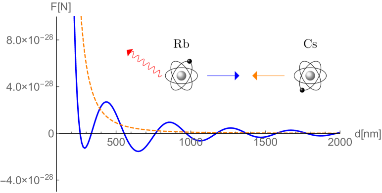
Figure 2: vdW interaction between one Cesium atom in the ground state ($5^{2}S_{1/2}$) and an excited Rubidium atom ($5^{2}P_{1/2}$). The thick line represents the force on Rubidium and the dashed one that on Cesium.

However our theory is more general because it includes the presence of general environments for the two atoms, like magnetodielectric bodies. Many differences arise in this more general case. Firstly the interaction can be described as a two-photon process, where the photons can be reflected by the body’s surface (see Fig. 3 ); this reflection is mathematically described in our formalism by the scattering Green tensor, which is known for many geometries and magnetodielectric properties. Secondly due to the presence of the additional body the action-reaction principle is also violated for ground-state atoms, with the interaction being accompanied by the transfer of linear momentum to the body. Lastly the total force acting on one molecule is not parallel to the interparticle separation vector.

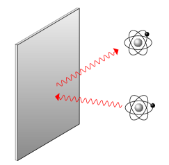
Figure 3: Body-assisted vdW interaction: the exchanged photons can be reflected by the body’s surface.

We see that the resonant contribution vanishes for times much larger than the atomic lifetimes ($\mathbf{F}_{A}^{\text{r}}\propto p_{n}^{A}\left(t\right)=e^{-\Gamma_{n}^{A}t}$), when the atoms have decayed to the ground-state. Fig. (4) represents this population-induced dynamics for the force acting on the excited Rubidium at a given distance.

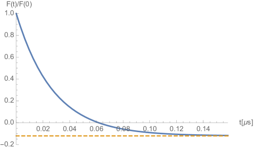
Figure 4: Population-induced dynamics for the vdW force acting on the excited Rubidium atom (thick line). The Rubidium atom is in the $5^{2}P_{1/2}$ state, while the Cesium is in the ground-state. The distance between the atoms is $r=10nm$.

We see that for time much larger than the atomic lifetime the force converges to the ground-state force, which is attractive. For times much smaller than the atomic lifetime the force is repulsive and roughly one order of magnitude larger than the ground-state force.

As stated above, the resonant force on the excited atom may be associated with photon recoil due to spontaneous emission. The fact that this force is stronger at small times can be understood from its ensemble-average nature: the probability of photon emission (and hence recoil) is highest for small times where a large fraction of the ensemble atoms are still in their excited state.

IV Comparison to Casimir–Polder force

Let us compare our result with the experimentally observed single-atom Casimir–Polder force. If an initially excited atom $A$ is placed near a magnetodielectric body, the resonant contribution, associated with a possible emission of a real photon, reads Buhmann2 :

$$\mathbf{F}_{A}^{r}\left(\mathbf{r}_{A},t\right)=\mu_{0}\sum\limits_{n\leqslant i_{A}}p_{n}^{A}\left(t\right)\sum\limits_{k<n}\left(\omega_{nk}^{A}\right)^{2}\\ \times\nabla_{A}\text{Re}\left\{\mathbf{d}_{nk}^{A}\cdot\mbox{{{{G}}}}^{1}\left(\mathbf{r}_{A},\mathbf{r}_{A},\omega_{nk}^{A}\right)\cdot\mathbf{d}_{kn}^{A}\right\}$$ (13)

where $\mbox{{{{G}}}}^{1}$ is the body’s scattering Green’s tensor. If the body is made up of ground-state atoms with polarizability $\bm{\alpha}_{B}\left(\omega\right)$ and positions $\textbf{r}_{B}$ and number density $\eta(\mathbf{r})$, it can be expressed in terms of a leading-order Born expansion born :

$$\mbox{{{{G}}}}^{1}\left(\mathbf{r}_{A},\mathbf{r}_{A},\omega\right)=\mu_{0}\omega^{2}\int\text{d}^{3}r_{B}\,\eta(\mathbf{r}_{B})\mbox{{{{G}}}}^{0}\left(\mathbf{r}_{A},\mathbf{r}_{B},\omega\right)\\ \cdot\bm{\alpha}_{B}\left(\omega\right)\cdot\mbox{{{{G}}}}^{0}\left(\mathbf{r}_{B},\mathbf{r}_{A},\omega\right)+...$$ (14)

where $\mbox{{{{G}}}}^{0}$ is the free-space Green’s tensor. The substitution of this expansion into the single-atom Casimir–Polder force leads to a resonant force

$$\mathbf{F}_{A}^{r}\left(\mathbf{r}_{A},t\right)=\int\text{d}^{3}r_{B}\,\eta(\mathbf{r}_{B})\mathbf{F}_{A}^{\mathrm{r}}\left(\mathbf{r}_{A},\mathbf{r}_{B}\right)\\ =\int\text{d}^{3}r_{B}\,\eta(\mathbf{r}_{B})\mu_{0}^{2}\sum\limits_{n\leqslant i_{A}}p_{n}^{A}(t)\sum\limits_{k<n}\nabla_{A}\operatorname{Re}\left\{\left(\omega_{nk}^{A}\right)^{4}\right.\mathbf{d}_{nk}^{A}\\ \cdot\mbox{{{{G}}}}^{1}\left(\mathbf{r}_{A},\mathbf{r}_{B},\omega_{nk}^{A}\right)\cdot\bm{\alpha}_{B}\left(\omega_{nk}^{A}\right)\left.\cdot\mbox{{{{G}}}}^{1}\left(\mathbf{r}_{B},\mathbf{r}_{A},\omega_{nk}^{A}\right)\cdot\mathbf{d}_{kn}^{A}\right\}$$ (15)

on the excited atom which is simply the sum over the (oscillating) resonant forces (LABEL:resonant) on the excited atom due to the ground-state atoms constituting the body. Note that a monotonous force contribution is absent from the single-atom Casimir–Polder force (15), as the atoms in the body are not excited. In the present combination of an excited atom interacting with a ground-state atom, we would expect the force on the body to contain a monotonous Casimir–Polder force component. However, the force on the body is usually not considered in the context of Casimir–Polder physics due to the strongly asymmetric mass ratio.

V Conclusions and outlook

Our dynamical theory has allowed us to study the vdW force involving excited atoms in generic environments. It is able to give a unique answer to the old puzzle whether the respective interaction is oscillating or monotonic, without recourse to ad hoc assumptions or prescriptions.

When one atom is excited we have shown that the van der Waals force acting on the excited atom indeed shows Drexhage-type oscillations, while the force acting on the ground-state atom is monotonic. We have explicitly demonstrated that the oscillating force is consistent with the respective Casimir–Polder force between an excited atom and a ground-state body. On the contrary, the monotonic forces components cannot be deduced from the atom–body force in this way, because they act on the atoms inside the body whereas Casimir–Polder calculations are usually restricted to calculating the force on the single atom in front of the body.

The oscillating force on the excited atom could have profound implications on the spatial correlations of excited atomic ensembles, in particular for Rydberg systems. In addition, both the oscillating and monotonous force components are expected to arise in waveguides as recently studied in Refs. Shamoon13 ; Shamoon14 ; ScheelHaakh ; Farina . It could be also interesting to generalize our model to include finite temperature, by chancing the fluctuation relations of the electromagnetic field, and to consider many-body vdW forces.

VI Appendix

VI.1 Perturbative expansion of the force operator

We consider the dynamics of an operator $\hat{\rho}(t)$, which is a superposition of operators $\hat{O}_{n}(t)$ with complex coefficients $f_{n}(t)$:

$$\hat{\rho}\left(t\right)=\sum\limits_{n}f_{n}\left(t\right)\hat{O}_{n}\left(t\right)$$ (16)

and we introduce a time limit which acts only on the operators:

$$\left.\hat{\rho}\left(t\right)\right|_{t\to t_{1}}=\sum\limits_{n}f_{n}\left(t\right)\hat{O}_{n}\left(t_{1}\right)$$ (17)

The operators $\hat{O}_{n}(t)$ evolve dynamically according to the Heisenberg equations:

$$\partial_{t}\hat{O}_{n}\left(t\right)=\frac{1}{\text{i}\hbar}\big{[}\hat{O}_{n}\left(t\right),\hat{H}\left(t\right)\big{]}$$ (18)

where $\hat{H}$ is the total Hamiltonian. This equation can be integrated from the initial time $t_{0}$ to a given time $t$:

$$\hat{O}_{n}\left(t\right)=\hat{O}_{n}\left(t_{0}\right)+\frac{1}{\text{i}\hbar}\int\limits_{t_{0}}^{t}\text{d}t_{1}\big{[}\hat{O}_{n}\left(t_{1}\right),\hat{H}\left(t_{1}\right)\big{]}$$ (19)

This equation shows that the dynamical evolution of the operators $\hat{\rho}$ is:

$$\hat{\rho}\left(t\right)=\left.\hat{\rho}\left(t\right)\right|_{t\to t_{0}}+\frac{1}{\text{i}\hbar}\int\limits_{t_{0}}^{t}\text{d}t_{1}\big{[}\left.\hat{\rho}\left(t\right)\right|_{t\to t_{1}},\hat{H}\left(t_{1}\right)\big{]}$$ (20)

The vdW force operator acting on the atom A, due to the presence of other atoms, is:

$$\hat{\mathbf{F}}_{A}(t)=\nabla\big{[}\hat{\mathbf{d}}_{A}\cdot\hat{\mathbf{E}}_{\not}{A}\left(\mathbf{r},t\right)\big{]}_{\mathbf{r}=\mathbf{r}_{A}}$$ (21)

where the field $\hat{\mathbf{E}}_{\not}{A}\left(\mathbf{r}_{A},t\right)$ represents the total electric field, excluding the radiation reaction of atom A. Using Eq. (20) we find the dynamical equation for the force:

$$\hat{\mathbf{F}}_{A}(t)=\hat{\mathbf{F}}_{A}(t)\big{|}_{t\to t_{0}}+\frac{1}{\text{i}\hbar}\int\limits_{t_{0}}^{t}\text{d}t_{1}\Big{[}\hat{\mathbf{F}}_{A}(t)\big{|}_{t\to t_{1}},\hat{H}\left(t_{1}\right)\Big{]}\\$$ (22)

This equation can be reiterated considering now the dynamics of the commutator $\Big{[}\hat{\mathbf{F}}_{A}(t)\big{|}_{t\to t_{1}},\hat{H}\left(t_{1}\right)\Big{]}$, which is a superposition of operators at the time $t_{1}$. Therefore, for weak coupling, we can construct a perturbative expansion $\hat{\mathbf{F}}_{A}(t)$ in terms of operators at the initial time $t_{0}$:

$$\hat{\mathbf{F}}_{A}\left(t\right)=\hat{\mathbf{F}}_{A}\left(t\right)\big{|}_{t\to t_{0}}\\ +\frac{1}{\text{i}\hbar}\int\limits_{t_{0}}^{t}\text{d}t_{1}\big{[}\hat{\mathbf{F}}_{A}\left(t\right)\big{|}_{t\to t_{1}},\hat{H}\left(t_{1}\right)\big{]}_{t_{1}\to t_{0}}\\ +\left(\frac{1}{\text{i}\hbar}\right)^{2}\int\limits_{t_{0}}^{t}\text{d}t_{1}\int\limits_{t_{0}}^{t_{1}}\text{d}t_{2}\\ \times\Big{[}\big{[}\hat{\mathbf{F}}_{A}\left(t\right)\big{|}_{t\to t_{1}},\hat{H}\left(t_{1}\right)\big{]}_{t_{1}\to t_{2}},\hat{H}\left(t_{2}\right)\Big{]}_{t_{2}\to t_{0}}+...$$ (23)

In our model the electric field and the flip-operators of the two atoms are the dynamical variables of the system. Two different time-scales are observed for the dynamical variables; there is a fast free dynamics and a much slower dynamics due to the interaction between the atoms and the field. For example the free evolution of the flip operators is on time scales of $\omega_{0}^{-1}=10^{-15}s$ while the dynamics due to the interaction is on time scales of $\Gamma^{-1}=10^{-9}s$. We define new dynamical variables according the formulas:

$$\hat{\mathbf{E}}^{\prime}\left(\mathbf{r},\omega,t\right)=\text{e}^{\text{i}\omega t}\hat{\mathbf{E}}\left(\mathbf{r},\omega,t\right)$$

$$\hat{A}^{\prime}_{mn}\left(t\right)=f_{mn}^{A}\left(-t\right)\hat{A}_{mn}\left(t\right)$$ (24)

where:

$$f_{mn}^{A}\left(t\right)=\mathrm{e}^{\big{[}\mathrm{i}\omega_{mn}^{A}-\left(\Gamma_{n}^{A}+\Gamma_{m}^{A}\right)/2\big{]}t}.$$ (25)

The new dynamical variables change on the time-scale of the interaction and have the following commutator with the total Hamiltonian (See Eq. 4, 5):

$$\left[\hat{\mathbf{E}}_{\not{A}}^{\prime}\left(\mathbf{r},\omega,t\right),\hat{H}\left(t\right)\right]=-\frac{\hbar\mu_{0}}{\pi}\text{e}^{\text{i}\omega t}$$

$$\times\sum\limits_{m,n}f_{mn}^{B}\left(t\right)\omega^{2}\text{Im}\mbox{{{{G}}}}\left(\mathbf{r},\mathbf{r}_{B},\omega\right)\mathbf{d}_{mn}^{B}\hat{B}_{mn}^{\prime}\left(t\right),$$

$$\left[\hat{A}_{mn}^{\prime}\left(t\right),\hat{H}\left(t\right)\right]=-\int\limits_{0}^{\infty}\text{d}\omega f_{mn}^{A}\left(-t\right)$$

$$\times\left(\text{e}^{-\text{i}\omega t}\mathbf{\hat{K}}_{mn}^{A}\left(t\right)\cdot\mathbf{\hat{E}}{{}^{\prime}}_{\not}{A}\left(\mathbf{r}_{A},\omega,t\right)\right.$$

$$\left.+\text{e}^{\text{i}\omega t}\mathbf{\hat{E}}{{}^{\prime}}_{\not}{A}^{\dagger}\left(\mathbf{r}_{A},\omega,t\right)\cdot\mathbf{\hat{K}}_{mn}^{A}\left(t\right)\right)$$ (26)

where:

$$\mathbf{\hat{K}}_{mn}^{A}\left(t\right)=\sum\limits_{k}\left(\hat{A}^{\prime}_{mk}\left(t\right)f_{mk}^{A}\left(t\right)\mathbf{d}_{nk}^{A}\right.\\ \left.-\hat{A}^{\prime}_{kn}\left(t\right)f_{kn}^{A}\left(t\right)\mathbf{d}_{km}^{A}\right)$$ (27)

and a normal ordering prescription is used.

From Eqs. (26) we see that the commutator between the Hamiltonian and a dynamical variable increases the number of electric dipole moments by one. Hence Eq. (23) represents a perturbative expansion of the force with the dipole element as perturbative parameter. In particular the electric vdW $N$-body force $\mathbf{F}_{A}\left(\mathbf{r}_{A},\mathbf{r}_{1}....,\mathbf{r}_{N-1}\right)$ acting on A due to the other atoms, with positions $\mathbf{r}_{1}....,\mathbf{r}_{N-1}$, contains $2N$ electric dipole matrix elements; this force results from the application of $2N-1$ commutators:

$$\mathbf{F}_{A}\left(\mathbf{r}_{A},\mathbf{r}_{1}....,\mathbf{r}_{N-1},t\right)\\ =\left(\frac{1}{\text{i}\hbar}\right)^{2N-1}\int\limits_{t_{0}}^{t}\text{d}t_{1}\int\limits_{t_{0}}^{t_{1}}\text{d}t_{2}...\int\limits_{t_{0}}^{t_{2N-2}}\text{d}t_{2N-1}\\ \times\Big{\langle}I\Big{|}\Bigg{[}\bigg{[}...\Big{[}\big{[}\mathbf{\hat{F}}_{A}\left(t\right)\big{|}_{t\to t_{1}},\hat{H}\left(t_{1}\right)\big{]}_{t_{1}\to t_{2}},\hat{H}\left(t_{2}\right)\Big{]}_{t_{2}\to t_{3}},\\ ...,\hat{H}\left(t_{2N-2}\right)\bigg{]}_{t_{2N-2}\to t_{2N-1}},\hat{H}\left(t_{2N-1}\right)\Bigg{]}_{t_{2N-1}\to t_{0}}\Big{|}I\Big{\rangle}$$ (28)

where the expectation value is taken over the atomic+ field free state $\big{|}I\big{\rangle}$. This approximate solution to the coupled dynamics is equivalent to an iterative use of the atom–field equations, and it is valid for weak coupling between atoms and field.

The expectation value on free atomic and field states can be easily performed, since after the limit $t_{2N-1}\to t_{0}$ the resulting operators are evaluated at the same initial time $t_{0}$, which represents the time at which the electric field and the atoms are uncoupled.

VI.2 Van der Waals interaction between two atoms

We consider now the vdW interaction between two atoms. We suppose that the atomic states are incoherent superpositions of energy eigenstates $\left|n^{A}\right\rangle$ and $\left|l^{B}\right\rangle$ and the state of the field is the ground state.

In normal ordering, the force operator (see Eq. 21) can be expressed in terms of the new dynamical variables:

$$\mathbf{\hat{F}}_{A}\left(t\right)=\sum\limits_{m,n}\int\limits_{0}^{\infty}\text{d}\omega f_{mn}^{A}\left(t\right)\text{e}^{-\text{i}\omega t}\\ \times\nabla\big{\{}\hat{A}^{\prime}_{mn}\left(t\right)\mathbf{d}_{mn}^{A}\cdot\mathbf{\hat{E}^{\prime}}_{\not{A}}\left(\mathbf{r},\omega,t\right)\big{\}}_{\mathbf{r}=\mathbf{r}_{A}}+\text{h.c.}$$ (29)

The two-body vdW interaction, which contains four electric dipole moments, involves three commutators:

$$\textbf{F}_{A}\left(\mathbf{r}_{A},\mathbf{r}_{B},t\right)=\left(\frac{1}{\text{i}\hbar}\right)^{3}\int\limits_{t_{0}}^{t}\text{d}t_{1}\int\limits_{t_{0}}^{t_{1}}\text{d}t_{2}\int\limits_{t_{0}}^{t_{2}}\text{d}t_{3}\\ \times\bigg{\langle}\bigg{[}\Big{[}\big{[}\hat{\mathbf{F}}_{A}\left(t\right)\big{|}_{t\to t_{1}},\hat{H}\left(t_{1}\right)\big{]}_{t_{1}\to t_{2}}\\ ,\hat{H}\left(t_{2}\right)\Big{]}_{t_{2}\to t_{3}},\hat{H}\left(t_{3}\right)\bigg{]}_{t_{3}\to t_{0}}\bigg{\rangle}$$ (30)

With the help of Eqs. (26), the commutators can be evaluated. For example the application of one and two commutators gives:

$$\frac{1}{\text{i}\hbar}\big{[}\hat{\mathbf{F}}_{A} \left(t\right)\big{|}_{t\to t_{1}},\hat{H}\left(t_{1}\right)\big{]}=\frac{\text{i}}{\hbar}\sum\limits_{m,n}\int\limits_{0}^{\infty}\text{d}\omega\int\limits_{0}^{\infty}\text{d}\omega^{\prime}\text{e}^{-\text{i}\omega t}f_{mn}^{A}\left(t-t_{1}\right)\nabla\Big{\{}\big{(}\text{e}^{-\text{i}\omega^{\prime}t_{1}}\mathbf{\hat{K}}_{mn}^{A}\left(t_{1}\right)\cdot\hat{\mathbf{E}}^{\prime}_{\not}{A}\left(\mathbf{r}_{A},\omega^{\prime},t_{1}\right)+$$

$$+\text{e}^{\text{i}\omega^{\prime}t_{1}}\mathbf{\hat{E}}{{}^{\prime}}_{\not}{A}^{\dagger}\left(\mathbf{r}_{A},\omega^{\prime},t_{1}\right)\cdot\mathbf{\hat{K}}_{mn}^{A}\left(t_{1}\right)\big{)}\mathbf{d}_{mn}^{A}\cdot\hat{\mathbf{E}}^{\prime}_{\not{A}}\left(\mathbf{r},\omega,t_{1}\right)\Big{\}}_{\mathbf{r}=\mathbf{r}_{A}}$$

$$+\frac{\text{i}\mu_{0}}{\pi}\sum\limits_{m,n,r,s}\int\limits_{0}^{\infty}\text{d}\omega\omega^{2}\text{e}^{-\text{i}\omega\left(t-t_{1}\right)}f_{mn}^{A}\left(t\right)f_{rs}^{B}\left(t_{1}\right)\nabla\Big{\{}\hat{A}^{\prime}_{mn}\left(t_{1}\right)\hat{B}^{\prime}_{rs}\left(t_{1}\right)\mathbf{d}_{mn}^{A}\cdot\operatorname{Im}\mbox{{{{G}}}}\left(\mathbf{r},\mathbf{r}_{B},\omega\right)\cdot\mathbf{d}_{rs}^{B}\Big{\}}_{\mathbf{r}=\mathbf{r}_{A}}+\text{h.c.}$$

$$\left(\frac{1}{\text{i}\hbar}\right)^{2}\Big{[}\big{[}\mathbf{\hat{F}}_{A} \left(t\right)\big{|}_{t\to t_{1}},\hat{H}\left(t_{1}\right)\big{]}_{t_{1}\to t_{2}},\hat{H}\left(t_{2}\right)\Big{]}=-\frac{\mu_{0}}{\pi\hbar}\sum\limits_{m,n,r,s}\int\limits_{0}^{\infty}\text{d}\omega\int\limits_{0}^{\infty}\text{d}\omega^{\prime}f_{mn}^{A}\left(t-t_{1}\right)f_{rs}^{B}\left(t_{2}\right)$$

$$\times\nabla\Big{\{}\omega{{}^{\prime 2}}\text{e}^{-\text{i}\omega t}\Big{[}\text{e}^{-\text{i}\omega^{\prime}\left(t_{1}-t_{2}\right)}\mathbf{\hat{K}}_{mn}^{A}\left(t_{1}\right)\big{|}_{t_{1}\to t_{2}}\cdot\operatorname{Im}\mbox{{{{G}}}}\left(\mathbf{r}_{A},\mathbf{r}_{B},\omega^{\prime}\right)\cdot\mathbf{d}_{rs}^{B}\hat{B}^{\prime}_{rs}\left(t_{2}\right)$$

$$-\text{e}^{\text{i}\omega^{\prime}\left(t_{1}-t_{2}\right)}\hat{B}^{\prime}_{rs}\left(t_{2}\right)\mathbf{d}_{rs}^{B}\cdot\operatorname{Im}\mbox{{{{G}}}}\left(\mathbf{r}_{B},\mathbf{r}_{A},\omega^{\prime}\right)\cdot\mathbf{\hat{K}}_{mn}^{A}\left(t_{1}\right)\big{|}_{t_{1}\to t_{2}}\Big{]}\mathbf{d}_{mn}^{A}\cdot\hat{\mathbf{E}}^{\prime}_{\not}{A}\left(\mathbf{r},\omega,t_{2}\right)$$

$$+\omega^{2}\text{e}^{-\text{i}\omega\left(t-t_{2}\right)}\Big{[}\text{e}^{-\text{i}\omega^{\prime}t_{1}}\mathbf{\hat{K}}_{mn}^{A}\left(t_{1}\right)\big{|}_{t_{1}\to t_{2}}\cdot\hat{\mathbf{E}}^{\prime}_{\not}{A}\left(\mathbf{r}_{A},\omega^{\prime},t_{2}\right)+$$

$$+\text{e}^{\text{i}\omega^{\prime}t_{1}}\mathbf{\hat{E}}{{}^{\prime}}_{\not}{A}^{\dagger}\left(\mathbf{r}_{A},\omega^{\prime},t_{2}\right)\cdot\mathbf{\hat{K}}_{mn}^{A}\left(t_{1}\right)\big{|}_{t_{1}\to t_{2}}\Big{]}\mathbf{d}_{mn}^{A}\cdot\operatorname{Im}\mbox{{{{G}}}}\left(\mathbf{r},\mathbf{r}_{B},\omega\right)\cdot\mathbf{d}_{rs}^{B}\hat{B}^{\prime}_{rs}\left(t_{2}\right)\Big{\}}_{\mathbf{r}=\mathbf{r}_{A}}$$

$$-\frac{\mu_{0}}{\pi\hbar}\sum\limits_{m,n,r,s}\int\limits_{0}^{\infty}\text{d}\omega\int\limits_{0}^{\infty}\text{d}\omega^{\prime}\text{e}^{-\text{i}\omega\left(t-t_{1}\right)}\omega^{2}\nabla\Big{\{}\big{[}f_{mn}^{A}\left(t-t_{2}\right)f_{rs}^{B}\left(t_{1}\right)\big{(}\text{e}^{-\text{i}\omega^{\prime}t_{2}}\mathbf{\hat{K}}_{mn}^{A}\left(t_{2}\right)\cdot\hat{\mathbf{E}}^{\prime}_{\not}{A}\left(\mathbf{r}_{A},\omega^{\prime},t_{2}\right)$$

$$+\text{e}^{\text{i}\omega^{\prime}t_{2}}\mathbf{\hat{E}}{{}^{\prime}}_{\not}{A}^{\dagger}\left(\mathbf{r}_{A},\omega^{\prime},t_{2}\right)\cdot\mathbf{\hat{K}}_{mn}^{A}\left(t_{2}\right)\big{)}\hat{B}^{\prime}_{rs}\left(t_{2}\right)+f_{mn}^{A}\left(t\right)f_{rs}^{B}\left(t_{1}-t_{2}\right)\hat{A}^{\prime}_{mn}\left(t_{2}\right)$$

$$\times\big{(}\text{e}^{-\text{i}\omega^{\prime}t_{2}}\mathbf{\hat{K}}_{rs}^{B}\left(t_{2}\right)\cdot\hat{\mathbf{E}}^{\prime}_{\not}{B}\left(\mathbf{r}_{B},\omega^{\prime},t_{2}\right)+\text{e}^{\text{i}\omega^{\prime}t_{2}}\mathbf{\hat{E}}{{}^{\prime}}_{\not}{B}^{\dagger}\left(\mathbf{r}_{B},\omega^{\prime},t_{2}\right)\cdot\mathbf{\hat{K}}_{rs}^{B}\left(t_{2}\right)\big{)}\Big{]}$$

$$\times\mathbf{d}_{mn}^{A}\cdot\operatorname{Im}\mbox{{{{G}}}}\left(\mathbf{r},\mathbf{r}_{B},\omega\right)\cdot\mathbf{d}_{rs}^{B}\Big{\}}_{\mathbf{r}=\mathbf{r}_{A}}+\text{h.c.}$$ (31)

The commutators between $\mathbf{\hat{K}}_{mn}$ and the Hamiltonian have not been considered since they lead to higher order corrections in the electric dipole $\textbf{d}^{A}$ and $\textbf{d}^{B}$.

We then evaluate the last commutator and take the expectation value on the atomic and field states. The thermal expectation value over the free field variables can be performed with the help of the following fluctuation relations for zero-temperature Buhmann ; Buhmann2 :

$$\Big{\langle}\mathbf{\hat{E}}^{\left(0\right)}\left(\mathbf{r},\omega,t\right)\mathbf{\hat{E}}^{\left(0\right){\dagger}}\left(\mathbf{r}^{\prime},\omega^{\prime},t\right)\Big{\rangle}$$

$$=\frac{\hbar\mu_{0}}{\pi}\textup{Im}\mbox{{{{G}}}}\left(\mathbf{r},\mathbf{r}^{\prime},\omega\right)\omega^{2}\delta\left(\omega-\omega^{\prime}\right)$$ (32)

After some algebra we obtain:

$$\mathbf{F}\left(\mathbf{r}_{A},\mathbf{r}_{B},t\right)=-\frac{i\mu_{0}^{2}}{2\pi^{2}\hbar}\sum\limits_{n,l}p_{n}^{A}(t)p_{l}^{B}(t)\sum\limits_{k,p}\int\limits_{0}^{\infty}\text{d}\omega\int\limits_{0}^{\infty}\text{d}\omega^{\prime}\omega^{2}\omega{{}^{\prime 2}}\nabla_{A}\mathbf{d}_{nk}^{A}\cdot\text{Im}\mbox{{{{G}}}}\left(\mathbf{r}_{A},\mathbf{r}_{B},\omega\right)\cdot\mathbf{d}_{pl}^{B}\\ \times\mathbf{d}_{lp}^{B}\cdot\text{Im}\mbox{{{{G}}}}\left(\mathbf{r}_{B},\mathbf{r}_{A},\omega^{\prime}\right)\cdot\mathbf{d}_{kn}^{A}\int\limits_{t_{0}}^{t}\text{d}t_{1}\int\limits_{t_{0}}^{t_{1}}\text{d}t_{2}\int\limits_{t_{0}}^{t_{2}}\text{d}t_{3}\\ \times\left\{\text{e}^{-\text{i}\omega\left(t-t_{1}\right)}\left(f_{nk}^{A}\left(t-t_{2}\right)-f_{kn}^{A}\left(t-t_{2}\right)\right)\left(\text{e}^{-\text{i}\omega^{\prime}\left(t_{2}-t_{3}\right)}f_{lp}^{B}\left(t_{1}-t_{3}\right)-\text{e}^{\text{i}\omega^{\prime}\left(t_{2}-t_{3}\right)}f_{pl}^{B}\left(t_{1}-t_{3}\right)\right)\right.\\ +\text{e}^{-\text{i}\omega\left(t-t_{1}\right)}\left(\text{e}^{-\text{i}\omega^{\prime}\left(t_{2}-t_{3}\right)}f_{nk}^{A}\left(t-t_{3}\right)-\text{e}^{\text{i}\omega^{\prime}\left(t_{2}-t_{3}\right)}f_{kn}^{A}\left(t-t_{3}\right)\right)\left(f_{lp}^{B}\left(t_{1}-t_{2}\right)-f_{pl}^{B}\left(t_{1}-t_{2}\right)\right)\\ +\text{e}^{-\text{i}\omega\left(t-t_{2}\right)}\left(f_{nk}^{A}\left(t-t_{1}\right)-f_{kn}^{A}\left(t-t_{1}\right)\right)\left(\text{e}^{-\text{i}\omega^{\prime}\left(t_{1}-t_{3}\right)}f_{lp}^{B}\left(t_{2}-t_{3}\right)-\text{e}^{\text{i}\omega^{\prime}\left(t_{1}-t_{3}\right)}f_{pl}^{B}\left(t_{2}-t_{3}\right)\right)\\ +\left.\text{e}^{-\text{i}\omega\left(t-t_{3}\right)}\left(\text{e}^{-\text{i}\omega^{\prime}\left(t_{1}-t_{2}\right)}-\text{e}^{\text{i}\omega^{\prime}\left(t_{1}-t_{2}\right)}\right)\left(f_{nk}^{A}\left(t-t_{1}\right)-f_{kn}^{A}\left(t-t_{1}\right)\right)f_{lp}^{B}\left(t_{2}-t_{3}\right)\right\}+\text{c.c.}$$ (33)

where $\nabla_{A}$ is now applied to both Green’s tensors (after exploiting their symmetry and introducing a factor $1/2$). The function $f$ was defined in Eq. (25) and $p_{n}^{A}(t)=\big{\langle}\hat{A}_{nn}\left(t\right)\big{\rangle}$ and $p_{l}^{B}(t)=\big{\langle}\hat{B}_{ll}\left(t\right)\big{\rangle}$ represent the atomic populations of the states $\left|n\right\rangle$ and $\left|l\right\rangle$. We have considered time-reversal symmetric systems where $\textbf{d}_{mn}$ is real ($\textbf{d}_{mn}=\textbf{d}_{nm}$), and reciprocal media ($\mbox{{{{G}}}}^{\text{T}}\left(\mathbf{r}_{A},\mathbf{r}_{B},\omega\right)=\mbox{{{{G}}}}\left(\mathbf{r}_{B},\mathbf{r}_{A},\omega\right)$).

With the exception of resonant cavity-QED scenarios, we can assume the quantity $\omega^{2}\textup{Im}\mbox{{{{G}}}}\left(\mathbf{r}_{B},\mathbf{r}_{A},\omega\right)$ to be sufficiently flat and to not exhibit any narrow peaks in vicinity of any atomic frequency (weak coupling). For weak coupling, we may evaluate the time-integral by means of the Markov approximation, extending the lower limit of the time integral to $t_{0}=-\infty$. The resulting integrals are not converging. In order to force the convergence we add an infinitesimal factor to the frequency $\omega$, $\omega\to\omega-\text{i}\epsilon$, where $\epsilon>0$. Note that the opposite sign convention for this infinitesimal factor would lead to divergent integrals. Time-integration leads to the energy denominators in Table 1 in the main text.

The frequency denominators can be combined:

$$1/D_{2}+1/D_{7}+1/D_{10}$$

$$=1/(\omega^{(-)}-\omega^{\prime}\big{)}(\omega^{\prime}+\omega_{kn}^{A(-)})(\omega^{\prime}+\omega_{pl}^{B(+)})$$

$$1/D_{3}+1/D_{6}+1/D_{11}$$

$$=1/(\omega^{(-)}+\omega^{\prime})(\omega^{\prime}+\omega_{kn}^{A(+)})(\omega^{\prime}+\omega_{pl}^{B(-)})$$

$$1/D_{1}+1/D_{9}=\frac{1}{(\omega^{(-)}+\omega^{\prime})(\omega_{kn}^{A(-)}+\omega_{pl}^{B(-)})}$$

$$\times\bigg{(}\frac{1}{\omega^{(-)}+\omega_{kn}^{A(-)}}+\frac{1}{\omega^{\prime}+\omega_{pl}^{B(-)}}\bigg{)}$$

$$1/D_{4}+1/D_{12}=\frac{1}{(\omega^{\prime}-\omega^{(-)})(\omega_{kn}^{A(+)}+\omega_{pl}^{B(+)})}$$

$$\times\bigg{(}\frac{1}{\omega^{(-)}-\omega_{kn}^{A(+)}}-\frac{1}{\omega^{\prime}+\omega_{pl}^{B(+)}}\bigg{)}$$

$$1/D_{5}=\frac{1}{(\omega^{(-)}-\omega^{\prime})(\omega_{kn}^{A(-)}+\omega_{pl}^{B(-)})}$$

$$\times\bigg{(}\frac{1}{\omega^{\prime}+\omega_{kn}^{A(-)}}-\frac{1}{\omega^{\left(-\right)}+\omega_{kn}^{A(-)}}\bigg{)}$$

$$1/D_{8}=\frac{1}{(\omega^{(-)}+\omega^{\prime})(\omega_{kn}^{A(+)}+\omega_{pl}^{B(+)})}$$

$$\times\bigg{(}\frac{1}{\omega^{\prime}+\omega_{kn}^{A(+)}}+\frac{1}{\omega^{\left(-\right)}-\omega_{kn}^{A(+)}}\bigg{)},$$ (34)

which implies:

$$\sum\limits_{i=1}^{16}{\frac{1}{{{D_{i}}}}}+{\text{c.c.}}=f_{1}\left({\omega^{\prime}}\right)\left({\frac{1}{{{\omega^{\left(-\right)}}+\omega^{\prime}}}+\frac{1}{{{\omega^{\left(+\right)}}-\omega^{\prime}}}}\right)\\ +f_{2}\left(\omega^{(-)}\right)\left({\frac{1}{{\omega^{\prime}+{\omega^{\left(-\right)}}}}+\frac{1}{{\omega^{\prime}-{\omega^{\left(-\right)}}}}}\right)+{\text{c.c.}}$$ (35)

where we have defined the following functions:

$$f_{1}\left(\xi\right)= \frac{1}{\left(\omega_{kn}^{A\left(+\right)}+\omega_{pl}^{B\left(+\right)}\right)\left(\xi+\omega_{kn}^{A\left(+\right)}\right)}$$

$$+\frac{1}{\left(\omega_{kn}^{A\left(-\right)}+\omega_{pl}^{B\left(-\right)}\right)\left(\xi+\omega_{pl}^{B\left(-\right)}\right)}$$

$$+\frac{1}{\left(\xi+\omega_{kn}^{A\left(+\right)}\right)\left(\xi+\omega_{pl}^{B\left(-\right)}\right)}$$

$$f_{2}\left(\xi\right)= \frac{1}{\left(\omega_{kn}^{A\left(+\right)}+\omega_{pl}^{B\left(+\right)}\right)\left(\xi-\omega_{kn}^{A\left(+\right)}\right)}$$

$$+\frac{1}{\left(\omega_{kn}^{A\left(-\right)}+\omega_{pl}^{B\left(-\right)}\right)\left(\xi+\omega_{kn}^{A\left(-\right)}\right)}$$

$$+\left(\frac{1}{\xi+\omega_{kn}^{A\left(-\right)}}-\frac{1}{\xi-\omega_{kn}^{A\left(+\right)}}\right)\frac{1}{\xi+\omega_{pl}^{B\left(-\right)}}$$ (36)

and $\omega_{kn}^{A\left(\pm\right)}=\omega_{kn}^{A}\pm\text{i}\left(\Gamma_{k}^{A}+\Gamma_{n}^{A}\right)/2$ , $\omega_{pl}^{B\left(\pm\right)}=\omega_{pl}^{B}\pm\text{i}\left(\Gamma_{p}^{B}+\Gamma_{l}^{B}\right)/2$, $\omega^{\left(\pm\right)}=\omega\pm\text{i}\epsilon$.

For the first term in Eq. (35) we integrate over $\omega$ and for the second term we integrate over $\omega^{\prime}$. We use the identity $\textup{Im}\mbox{{{{G}}}}=\left(\mbox{{{{G}}}}-\mbox{{{{G}}}}^{*}\right)/2\mathrm{i}$ and the Schwarz reflection principle for the Green tensor:

$$\int\limits_{0}^{\infty}\mathrm{d}\omega^{\prime}\omega^{\prime 2}\left(\frac{1}{\omega^{\prime}+\omega^{(-)}}+\frac{1}{\omega^{\prime}-\omega^{(-)}}\right)\textup{Im}\mbox{{{{G}}}}\left(\mathbf{r}_{A},\mathbf{r}_{B},\omega^{\prime}\right)$$

$$=\frac{1}{2\mathrm{i}}\int\limits_{-\infty}^{\infty}\mathrm{d}\omega^{\prime}\omega^{\prime 2}\left(\frac{1}{\omega^{\prime}+\omega^{(-)}}+\frac{1}{\omega^{\prime}-\omega^{(-)}}\right)\mbox{{{{G}}}}\left(\mathbf{r}_{A},\mathbf{r}_{B},\omega^{\prime}\right)$$ (37)

The Green’s tensor is analytic in the upper half of the complex plane, including the real axis, and it is also finite at the origin. We close the path with an infinitely large half-circle in the upper complex half-plane and take the residuum inside the path. The integral along the infinite semi-circle vanishes for $\textbf{r}_{A}\neq\textbf{r}_{B}$ because:

$$\mathop{\lim}\limits_{\left|\omega\right|\to+\infty}\omega^{2}\left.\mbox{{{{G}}}}\left(\mathbf{r}_{A},\mathbf{r}_{B},\omega\right)\right|_{\mathbf{r}_{A}\neq\mathbf{r}_{B}}=0$$ (38)

We thus find:

$$\int\limits_{0}^{\infty}\mathrm{d}\omega^{\prime}\omega^{\prime 2}\left(\frac{1}{\omega^{\prime}+\omega^{(-)}}+\frac{1}{\omega^{\prime}-\omega^{(-)}}\right)\textup{Im}\mbox{{{{G}}}}\left(\mathbf{r}_{A},\mathbf{r}_{B},\omega^{\prime}\right)\\ \simeq\pi\omega^{2}\mbox{{{{G}}}}\left(\mathbf{r}_{A},\mathbf{r}_{B},-\omega\right)$$ (39)

The total force can be expressed as sum of two terms:

$$\mathbf{F}_{A}\left(\mathbf{r}_{A},\mathbf{r}_{B},t\right)=\mathbf{F}_{A}^{1}\left(\mathbf{r}_{A},\mathbf{r}_{B},t\right)+\mathbf{F}_{A}^{2}\left(\mathbf{r}_{A},\mathbf{r}_{B},t\right)$$

$$\mathbf{F}_{A}^{1}\left(\mathbf{r}_{A},\mathbf{r}_{B},t\right)= \frac{\mu_{0}^{2}}{2\pi\hbar}\sum\limits_{n,l}p_{n}^{A}(t)p_{l}^{B}(t)\sum\limits_{k,p}\int\limits_{0}^{\infty}\text{d}\omega\omega^{4}$$

$$\times\nabla_{A}\text{Im}\left\{\left(\mathbf{d}_{nk}^{A}\cdot\mbox{{{{G}}}}\left(\mathbf{r}_{A},\mathbf{r}_{B},\omega\right)\cdot\mathbf{d}_{pl}^{B}\right)^{2}g_{1}\left(\omega\right)\right\}$$

$$\mathbf{F}_{A}^{2}\left(\mathbf{r}_{A},\mathbf{r}_{B},t\right)= \frac{\mu_{0}^{2}}{2\pi\hbar}\sum\limits_{n,l}p_{n}^{A}(t)p_{l}^{B}(t)\sum\limits_{k,p}\int\limits_{0}^{\infty}\text{d}\omega\omega^{4}$$

$$\times\nabla_{A}\left\{\left|\mathbf{d}_{nk}^{A}\cdot\mbox{{{{G}}}}\left(\mathbf{r}_{A},\mathbf{r}_{B},\omega\right)\cdot\mathbf{d}_{pl}^{B}\right|^{2}g_{2}\left(\omega\right)\right\}$$ (40)

where:

$$g_{1}\left(\omega\right)=f_{1}^{*}\left(\omega\right)+f_{2}^{*}\left(\omega\right)=\\ \frac{1}{\omega+\omega_{pl}^{B\left(+\right)}}\left(\frac{1}{\omega+\omega_{kn}^{A\left(+\right)}}\right.\\ \left.+\frac{1}{\omega+\omega_{kn}^{A\left(-\right)}}-\frac{1}{\omega-\omega_{kn}^{A\left(-\right)}}\right)\\ +\frac{1}{\omega_{kn}^{A\left(+\right)}+\omega_{pl}^{B\left(+\right)}}\left(\frac{1}{\omega+\omega_{kn}^{A\left(+\right)}}+\frac{1}{\omega+\omega_{pl}^{B\left(+\right)}}\right)\\ +\frac{1}{\omega_{kn}^{A\left(-\right)}+\omega_{pl}^{B\left(-\right)}}\left(\frac{1}{\omega+\omega_{kn}^{A\left(-\right)}}+\frac{1}{\omega-\omega_{kn}^{A\left(-\right)}}\right)$$ (41)

and:

$$g_{2}\left(\omega\right)=\text{Im}\left[f_{1}\left(\omega\right)+f_{2}\left(\omega\right)\right]\\ =2\operatorname{Re}\left[\frac{1}{\omega_{kn}^{A\left(+\right)}+\omega}+\frac{1}{\omega_{kn}^{A\left(+\right)}-\omega}\right]\text{Im}\frac{1}{\omega+\omega_{pl}^{B\left(-\right)}}$$ (42)

We consider then the limiting case of vanishing line-widths:

$$\varepsilon_{A}= \left(\Gamma_{n}^{A}+\Gamma_{k}^{A}\right)/2\to 0^{+}$$

$$\varepsilon_{B}= \left(\Gamma_{l}^{A}+\Gamma_{p}^{B}\right)/2\to 0^{+}$$ (43)

In this limit the function $g_{1}$ can be simplified:

$$\mathop{\lim}\limits_{\epsilon_{A,B}\to 0^{+}}g_{1}\left(\omega\right)=\frac{4\left(\omega-\omega_{kn}^{A}\right)\left(\omega+\omega_{kn}^{A}\right)}{\left(\left(\omega+\omega_{kn}^{A}\right)^{2}+\varepsilon_{A}^{2}\right)\left(\omega-\omega_{kn}^{A}+\text{i}\varepsilon_{A}\right)}\\ \times\frac{\left(\omega+\omega_{kn}^{A}+\omega_{pl}^{B}\right)}{\left(\omega+\omega_{pl}^{B}+\text{i}\varepsilon_{B}\right)\left(\omega_{kn}^{A}+\omega_{pl}^{B}\right)}$$ (44)

Using the property $\frac{1}{x\pm\text{i}\varepsilon}=\mathcal{P}\frac{1}{x}\mp\text{i}\pi\delta\left(x\right)$, where $\mathcal{P}$ is the principal value, we can also simplify $g_{2}$ :

$$g_{2}\left(\omega\right)=2\pi\operatorname{Re}\Bigg{[}\frac{1}{\omega_{kn}^{A\left(+\right)}+\omega}+\frac{1}{\omega_{kn}^{A\left(+\right)}-\omega}\Bigg{]}\delta\left({\omega-\omega_{lp}^{B}}\right)$$ (45)

With these results, after performing a Wick rotation on the imaginary axis we find the following non resonant and resonant contributions to the $\textbf{F}_{A}^{1}$:

$$\mathbf{F}_{A}^{1}\left(\mathbf{r}_{A},\mathbf{r}_{B},t\right)=\frac{\mu_{0}^{2}}{2\pi\hbar}\sum\limits_{n,l}p_{n}^{A}(t)p_{l}^{B}(t)\sum\limits_{k,p}\int\limits_{0}^{\infty}\text{d}\xi\xi^{4}\\ \times\frac{g_{1}\left(\text{i}\xi\right)+g_{1}^{*}\left(-\text{i}\xi\right)}{2}\nabla_{A}\left\{\left(\mathbf{d}_{nk}^{A}\cdot\mbox{{{{G}}}}\left(\mathbf{r}_{A},\mathbf{r}_{B},\text{i}\xi\right)\cdot\mathbf{d}_{pl}^{B}\right)^{2}\right\}\\ +\frac{\mu_{0}^{2}}{2\hbar}\sum\limits_{n,l}p_{n}^{A}(t)p_{l}^{B}(t)\sum\limits_{k,p}\\ \times\nabla_{A}\Big{\{}\text{Res}_{1}\big{[}g_{1}\left(\omega\right)\omega^{4}\left(\mathbf{d}_{nk}^{A}\cdot\mbox{{{{G}}}}\left(\mathbf{r}_{A},\mathbf{r}_{B},\omega\right)\cdot\mathbf{d}_{pl}^{B}\right)^{2}\big{]}\\ -\text{Res}_{2}\big{[}g_{1}^{*}\left(-\omega\right)\omega^{4}\left(\mathbf{d}_{nk}^{A}\cdot\mbox{{{{G}}}}\left(\mathbf{r}_{A},\mathbf{r}_{B},\omega\right)\cdot\mathbf{d}_{pl}^{B}\right)^{2}\big{]}\Big{\}}$$ (46)

where $\text{Res}_{1}$ indicates the sum of the residues in the first quadrant, and $\text{Res}_{2}$ the sum of the residues in the second quadrant. Similarly, $\textbf{F}_{A}^{2}$ reduces to

$$\mathbf{F}_{A}^{2}\left(\mathbf{r}_{A},\mathbf{r}_{B},t\right)=\mu_{0}^{2}\sum\limits_{l}p_{l}^{B}(t)\sum\limits_{p<l}\left(\omega_{lp}^{B}\right)^{4}\nabla_{A}\\ \times\left\{\mathbf{d}_{lp}^{B}\cdot\mbox{{{{G}}}}\left(\mathbf{r}_{B},\mathbf{r}_{A},\omega_{lp}^{B}\right)\cdot\bm{\alpha}_{A}\left(\omega_{lp}^{B}\right)\cdot{\mbox{{{{G}}}}^{*}}\left(\mathbf{r}_{A},\mathbf{r}_{B},\omega_{lp}^{B}\right)\cdot\mathbf{d}_{pl}^{B}\right\}\\$$ (47)

where $\bm{\alpha}_{A}$ is the polarizability of the excited atom A. The sum of $\textbf{F}_{A}^{1}$ and $\textbf{F}_{A}^{2}$ gives the non-resonant and resonant contributions of the total vdW force, see Eqs. (9) and (LABEL:resonant).

References

• (1) H. B. G. Casimir, Proc. K. Ned. Akad. Wet. 51, 793 (1948).
• (2) H. B. G. Casimir and D. Polder, Phys. Rev. 73, 360 (1948).
• (3) T. Kihara, Intermolecular forces (John Wiley & Sons, New York, 1977).
• (4) S. Nir, Prog. Surf. Sci. 8, 1 (1976).
• (5) J. de Pater, J.J. Lissauer Planetary Sciences, Cambridge University Press, Cambridge (2010).
• (6) J. Preto, M. Pettini and J. A. Tuszynski, Phys. Rev. E 91, 052710 (2015).
• (7) F. M. Serry, D. Walliser and G. J. Maclay, J. Appl. Phys. 84, 2501 (1998).
• (8) M. A. Wilson, P. Bushev, J. Eschner, F. Schmidt-Kaler, C. Becher, R. Blatt, and U. Dorner, Phys. Rev. Lett. 91, 213602 (2003).
• (9) P. Bushev, A. Wilson, J. Eschner, C. Raab, F. Schmidt-Kaler, C. Becher, and R. Blatt, Phys. Rev. Lett. 92, 223602 (2004).
• (10) S. Y. Buhmann, Dispersion forces I (Springer, Heidelberg, 2012).
• (11) E. A. Power, T. Thirunamachandran, Phys. Rev. A 47, 2539 (1993).
• (12) L. Gomberoff, R. R. McLone, E. A. Power, J. Chem. Phys. 44, 4148 (1966).
• (13) R. R. McLone, E. A. Power, Proc. R. Soc. Lond. Ser. A 286, 573 (1965).
• (14) M. R. Philpott, Proc. Phys. Soc. Lond. 87, 619 (1966).
• (15) E. A. Power, T. Thirunamachandran, Phys. Rev. A 51, 3660 (1995).
• (16) E. A. Power, T. Thirunamachandran, Chem. Phys. 171, 1 (1993).
• (17) Y. Sherkunov, Phys. Rev. A 75, 012705 (2007).
• (18) M. Donaire, R. Guérout, A. Lambrecht, Phys. Rev. Lett. 115, 033201 (2015).
• (19) P. R. Berman, Phys. Rev. A 91, 042127 (2015).
• (20) L. Rizzuto, R. Passante, F. Persico, Phys. Rev. A 70, 012107 (2004).
• (21) H.R. Haakh, J. Schiefele, and C. Henkel, Int. J. Mod. Phys.: Conf. Ser. 14, 347 (2012).
• (22) P.W. Milonni and S. M. H. Rafsanjani, Phys. Rev. A 92, 062711 (2015).
• (23) M. Donaire, arXiv:1603.08195 (2016).
• (24) M. Donaire, arXiv:1604.07071 (2016).
• (25) S. Scheel, S. Y. Buhmann, C. Clausen, and P. Schneeweiss Phys. Rev. A 92, 043819 (2015).
• (26) H. Safari and M. R. Karimpour, Phys. Rev. Lett. 114, 013201 (2015).
• (27) S. Y. Buhmann and D. G. Welsch, Prog. Quantum Electron. 31, 51 (2007).
• (28) S. Y. Buhmann, Dispersion Forces II (Springer, Heidelberg, 2013).
• (29) L. Knöll, S. Scheel, D.-G. Welsch, QED in Dispersing and Absorbing Media in J. Peřina (ed.) Coherence and Statistics of Photons and Atoms, p. 1 (Wiley, New York, 2001).
• (30) J. R. Ackerhalt, P. L. Knight, and J. H. Eberly, Phys. Rev. Lett. 30, 456 (1973).
• (31) D. A. Steck, Rubidium 87D Line Data, Cesium D Line Data http://steck.us/alkalidata (2009).
• (32) S. Y. Buhmann and Welsch, Appl. Phys. B 82, 189 (2006).
• (33) E. Shahmoon and G. Kuritzki, Phys. Rev. A 87, 062105 (2013).
• (34) E. Shahmoon, I. Mazets and G. Kurizki, Proc. Nat. Akad. Sci. 111, 10485 (2013).
• (35) H. R. Haakh and S. Scheel, Phys. Rev. A 91, 052707 (2015).
• (36) R. de Melo de Souza, W. J. M. Kort-Kamp, F. S. S. Rosa and C. Farina, Phys. Rev. A 91, 052708 (2015).