Ab Initio Theory of Superconductivity in a Magnetic Field I. : Spin Density Functional Theory For Superconductors and Eliashberg Equations.

Abstract

We present a first-principles approach to describe magnetic and superconducting systems and the phenomena of competition between these electronic effects. We develop a density functional theory: SpinSCDFT, by extending the Hohenberg-Kohn theorem and constructing the non-interacting Kohn-Sham system. An exchange-correlation functional for SpinSCDFT is derived from the Sham Schlüter connection between the SpinSCDFT Kohn-Sham and a self-energy in Eliashberg approximation. The reference Eliashberg equations for superconductors in the presence of magnetism are also derived and discussed.

I Introduction

In this work, we present how magnetic (M) and superconducting (SC) properties can be computed on the same footing and from first principles by extending the Density Functional Theory (DFT) framework. In developing this spin DFT for SC (SpinSCDFT) we will restrict ourselves to situations where currents are negligible and only consider the effect of the Zeeman term of the Hamiltonian. Under this assumption we can exclude the occurrence of the Abrikosov vortex state Abrikosov (1957), that having a mesoscopic characteristic length-scale would be beyond the present computational power for a fully ab-initio method.

The expulsion of static M fields from the bulk Walther Meissner (1933) is one of the most spectacular properties of SC materials and illustrates the profound competition between M and SC behavior. The SC-M interaction generates in fact a large number of interesting phenomena on which the scientific community has focused attention. Some of the most investigated are the Abrikosov vorticesAbrikosov (1957) and the variety of fascinating effects occurring in heterostructuresSatapathy et al. (2012), such as stacked layers of M with SC material (see Ref. Buzdin, 2005 for a review). Among these effects is the FFLO state, named after Fulde, Ferrel Fulde and Ferrell (1964), Larkin and Ovchinnikov Larkin , where strong exchange fields induce a SC state with a finite momentum pairing. This state was recently observed experimentally Bianchi et al. (2003); Lortz et al. (2007) in heavy Fermion SC, many years after its prediction. In addition, triplet SC has been observed in several systemsSigrist and Ueda (1991); Jérome et al. (1980); Rice and Sigrist (1995); Luke et al. (1998); Ishida et al. (1998); Saxena et al. (2000); Bauer et al. (2004), and is usually associated to ferromagnetism.

Among the many effects generated by the interplay of magnetism and superconductivity, some have an intrinsic microscopic nature and could be accessible to first-principle calculations, in particular we refer to the sharp suppression of the critical temperature due to paramagnetic impuritiesAbrikosov and Gor’kov (1961), and the surprising evidence of coexisting phases between singlet SC and local magnetism, in particular close to a magnetic phase boundary Felner et al. (1997); Dikin et al. (2011); Saxena et al. (2000); Aoki et al. (2001) where high$-T_{c}$ SC occurs Manske (2004); Lee et al. (2006). We devote this work to set the ground for an ab-initio theory to describe these physical effects.

We will start our formulation from the Pauli Hamiltoninan (Sec. II). In Sec. (III), we formulate a density functional theory (DFT), proving that the electronic density $n(\boldsymbol{r})$ , the spin magnetization $\boldsymbol{m}(\boldsymbol{r})$, the diagonal of the nuclear $N$-body density matrix and the singlet and triplet SC order parameters $\boldsymbol{\chi}(\boldsymbol{r},\boldsymbol{r}^{\prime})$ are uniquely connected with their respective external potentials. With this extension of the Hohenberg-Kohn theorem Hohenberg and Kohn (1964) we lay the foundation of the DFT for M and SC systems: SpinSCDFT. In Sec. III.1 we introduce the formally non-interacting Kohn Sham (KS) system that reproduces the exact densities of the interacting system. Similar to every DFT, SpinSCDFT relies on the construction of an exchange correlation ($xc$) functional that connects the KS with the interacting system. In this work, this is achieved by establishing, in Sec. III.2, a Sham-Schlüter connection Sham and Schlüter (1983) via the Dyson equation of the interacting system.

The interacting system is also being investigated directly by means of a magnetic extension of the Eliashberg method Vonsovsky et al. (1982); Allen and Mitrović (1983); Sanna et al. (2012); Carbotte (1990); Eliashberg (1960). A derivation of this alternative approach in the present notation is given in Sec. IV. Advantages and disadvantages of these two theoretical schemes, SpinSCDFT and Eliashberg, will be discussed in the conclusions.

II Hamiltonian

We assume that the interacting system is governed by the Pauli Hamiltonian (we use Hartree atomic units throughout)

$$\hat{H}=\hat{T}_{{\rm{\scriptscriptstyle e}}}+\hat{T}_{{\rm{\scriptscriptstyle n}}}+\hat{V}_{{\scriptscriptstyle{\rm e}}}+\hat{U}_{{\rm{\scriptscriptstyle ee}}}+\hat{U}_{{\rm{\scriptscriptstyle en}}}+\hat{U}_{{\rm{\scriptscriptstyle nn}}}\,,$$ (1)

where $\hat{T}_{{\rm{\scriptscriptstyle e}}}$ ($\hat{T}_{{\rm{\scriptscriptstyle n}}}$) is the kinetic energy operator of the electron (nuclei) and $\hat{U}_{{\rm{\scriptscriptstyle ee}}}$($\hat{U}_{{\rm{\scriptscriptstyle nn}}}$) is the electron-electron (nuclei-nuclei) interaction, i.e. usually the Coulomb potential. $\hat{U}_{{\rm{\scriptscriptstyle en}}}$ is the Coulomb potential between electrons and nuclei. To break the respective symmetries and allow the corresponding densities to adopt non-zero values in a thermal average we include an external vector potential $\boldsymbol{A}_{{\rm{\scriptscriptstyle ext}}}(\boldsymbol{r})$ and an external singlet/triplet pair potential $\boldsymbol{\varDelta}^{{\rm{\scriptscriptstyle ext}}}(\boldsymbol{r},\boldsymbol{r}^{\prime})$ in the Hamiltonian. These external fields will be set to zero at the end of the derivation. Because we do not consider currents, the only term in the Pauli Hamiltonian containing $\boldsymbol{A}_{{\rm{\scriptscriptstyle ext}}}(\boldsymbol{r})$ is:

$$\hat{T}_{{\rm{\scriptscriptstyle e}}}=\int{\rm d}\boldsymbol{r}\,\hat{\psi}^{\dagger}(\boldsymbol{r})\cdot\Bigl{(}-\sigma_{0}\frac{\boldsymbol{\nabla}^{2}}{2}+\mathbf{S}\cdot\boldsymbol{B}_{{\scriptscriptstyle{\rm ext}}}(\boldsymbol{r})\Bigr{)}\cdot\hat{\psi}(\boldsymbol{r})$$ (2)

with $\boldsymbol{B}_{{\scriptscriptstyle{\rm ext}}}(\boldsymbol{r})=\boldsymbol{\nabla}\times\boldsymbol{A}_{{\rm{\scriptscriptstyle ext}}}(\boldsymbol{r})$ and $\mathbf{S}=\frac{1}{2}(\begin{array}[]{ccc}\sigma_{x}&\sigma_{y}&\sigma_{z}\end{array})^{{\rm T}}$, $\sigma_{x,y,z}$ being the Pauli matrices. We use the notation $\hat{\psi}^{\dagger}(\boldsymbol{r})=\bigl{(}\begin{array}[]{cc}\hat{\psi}^{\dagger}(\boldsymbol{r}\uparrow)&\hat{\psi}^{\dagger}(\boldsymbol{r}\downarrow)\end{array}\bigr{)}$ for the field operator where $\hat{\psi}^{\dagger}(\boldsymbol{r}\uparrow)$ creates an electron at location $\boldsymbol{r}$ with spin up. The scalar potential part of $\hat{H}$ reads:

$$\hat{V}_{{\scriptscriptstyle{\rm e}}} = \int{\rm d}\boldsymbol{r}\,\hat{\psi}^{\dagger}(\boldsymbol{r})\cdot\sigma_{0}\cdot\hat{\psi}(\boldsymbol{r})v_{{\scriptscriptstyle{\rm ext}}}(\boldsymbol{r})$$ (3)

$$\!\!-\frac{1}{2}\int{\rm d}\boldsymbol{r}\int{\rm d}\boldsymbol{r}^{\prime}\Bigl{(}\hat{\boldsymbol{\chi}}(\boldsymbol{r},\boldsymbol{r}^{\prime})\cdot\boldsymbol{\varDelta}^{{\rm{\scriptscriptstyle ext}}\ast}(\boldsymbol{r},\boldsymbol{r}^{\prime})+{\rm h.c.}\Bigr{)}\,.$$

Here, the anomalous density operator is defined by

$$\hat{\boldsymbol{\chi}}(\boldsymbol{r},\boldsymbol{r}^{\prime}) = \hat{\psi}(\boldsymbol{r})\cdot\boldsymbol{\Phi}\cdot\hat{\psi}(\boldsymbol{r}^{\prime})\,.$$ (4)

$\hat{\boldsymbol{\chi}}(\boldsymbol{r},\boldsymbol{r}^{\prime})$ is a 4-vector of which the first component (proportional to $\Phi_{1}$) is the singlet part of the order parameter, while the other components (related to $\Phi_{2}$,$\Phi_{3}$ and $\Phi_{4}$) are the triplet part. The 4 components of the singlet/triplet vector $\boldsymbol{\Phi}=(\mbox{i}\sigma_{y},-\sigma_{z},\sigma_{0},\sigma_{x})^{{\rm T}}$ are $2\times 2$ spin matrices similar to the components of $\mathbf{S}$. Similarly, the anomalous external potential

$$\boldsymbol{\varDelta}^{{\rm{\scriptscriptstyle ext}}}(\boldsymbol{r},\boldsymbol{r}^{\prime}) = \left(\begin{array}[]{c}\varDelta_{{\rm s}}^{{\rm{\scriptscriptstyle ext}}}(\boldsymbol{r},\boldsymbol{r}^{\prime})\\ \varDelta_{{\rm tx}}^{{\rm{\scriptscriptstyle ext}}}(\boldsymbol{r},\boldsymbol{r}^{\prime})\\ \varDelta_{{\rm ty}}^{{\rm{\scriptscriptstyle ext}}}(\boldsymbol{r},\boldsymbol{r}^{\prime})\\ \varDelta_{{\rm tz}}^{{\rm{\scriptscriptstyle ext}}}(\boldsymbol{r},\boldsymbol{r}^{\prime})\end{array}\right)$$ (9)

is assumed to have singlet and triplet components.

III Spin SCDFT

The conventional density functional approach to the Many-Body problem Hohenberg and Kohn (1964); Kohn and Sham (1965); Runge and Gross (1984); Kreibich and Gross (2001) consists of two steps: first establishing the Hohenberg Kohn (HK) theorem, i.e.  realize that a chosen set of densities is uniquely connected with a set of external potentials; second, construct an auxiliary, non-interacting KS system to reproduce the densities of the interacting system.

We follow Ref. Lüders et al., 2005 and consider a multi-component DFT with the normal $n(\boldsymbol{r})$, the SC order parameter as the anomalous density $\boldsymbol{\chi}(\boldsymbol{r},\boldsymbol{r}^{\prime})$, that describes the electrons condensed into singlet and triplet states, and $\varGamma(\boldsymbol{R}_{1}..\boldsymbol{R}_{N})$ the diagonal of the nuclear $N$-body density matrix. In addition, we introduce the magnetization $\boldsymbol{m}(\boldsymbol{r})$ as another electronic density.

The HK proof $\bigl{(}n(\boldsymbol{r}),\boldsymbol{m}(\boldsymbol{r}),\boldsymbol{\chi}(\boldsymbol{r},\boldsymbol{r}^{\prime}),\varGamma(\boldsymbol{R}_{1}..\boldsymbol{R}_{N})\bigr{)}\leftrightarrow\bigl{(}v_{{\rm{\scriptscriptstyle ext}}}(\boldsymbol{r}),\boldsymbol{B}_{{\rm{\scriptscriptstyle ext}}}(\boldsymbol{r}),\boldsymbol{\varDelta}^{{\rm{\scriptscriptstyle ext}}}(\boldsymbol{r},\boldsymbol{r}^{\prime}),W_{{\rm{\scriptscriptstyle ext}}}(\boldsymbol{R}_{1}..\boldsymbol{R}_{N})\bigr{)}$ is a straightforward generalization of Mermin’s HK proof in a finite temperature ensembleMermin (1965). For this reason we will not repeat it here. On the other hand the construction of the KS system is done assuming that densities are always $v-$representable i.e. we assume the existence of the KS system. Being non-interacting it consists of independent equations for nuclei and electrons, coupled only via the $xc$ potentials. Our focus will be on the electronic system, discussed in detail in Sec. III.1.2. The nuclear part will be addressed in Sec. III.1.1, briefly, since it is usually enough to approximate the nuclear KS system with its non SC counterpartLüders et al. (2005); Marques et al. (2005). The construction the $xc$ potentials will be discussed in Sec. III.2 and Sec. III.3.

III.1 The Kohn-Sham System

In this work we are mainly interested in the influence of a magnetic field on the SC state. We briefly review the approximation steps to arrive at the Fröhlich Hamiltonian starting from the formally exact multi-component DFT. The reader may refer to the existing literature for further detailsLüders et al. (2005); Kreibich and Gross (2001). We introduce the KS Hamiltonian

$$\hat{H}_{{\scriptscriptstyle{\rm KS}}}=\hat{H}_{{\scriptscriptstyle{\rm KS}}}^{{\rm{\scriptscriptstyle e}}}+\hat{H}_{{\scriptscriptstyle{\rm KS}}}^{{\scriptscriptstyle{\rm n}}}\,,$$ (10)

where we have separated the electronic $\hat{H}_{{\scriptscriptstyle{\rm KS}}}^{{\rm{\scriptscriptstyle e}}}$

$$\hat{H}_{{\scriptscriptstyle{\rm KS}}}^{{\rm{\scriptscriptstyle e}}} = \int{\rm d}\boldsymbol{r}\,\hat{\psi}^{\dagger}(\boldsymbol{r})\cdot\sigma_{0}\Bigl{(}-\frac{\boldsymbol{\nabla}^{2}}{2}+v_{{\scriptscriptstyle{\rm s}}}(\boldsymbol{r})-\mu\Bigr{)}\cdot\hat{\psi}(\boldsymbol{r})$$ (11)

$$-\frac{1}{2}\int{\rm d}\boldsymbol{r}\int{\rm d}\boldsymbol{r}^{\prime}\Bigl{(}\hat{\boldsymbol{\chi}}(\boldsymbol{r},\boldsymbol{r}^{\prime})\cdot\boldsymbol{\varDelta}^{{\scriptscriptstyle{\rm s}}\ast}(\boldsymbol{r},\boldsymbol{r}^{\prime})+{\rm h.c.}\Bigr{)}$$

$$+\int{\rm d}\boldsymbol{r}\,\hat{\boldsymbol{m}}(\boldsymbol{r})\cdot\boldsymbol{B}_{{\scriptscriptstyle{\rm s}}}(\boldsymbol{r})\,,$$

from the nuclear $\hat{H}_{{\scriptscriptstyle{\rm KS}}}^{{\scriptscriptstyle{\rm n}}}$

$$\hat{H}_{{\scriptscriptstyle{\rm KS}}}^{{\scriptscriptstyle{\rm n}}} = -\int{\rm d}\boldsymbol{R}\,\hat{\zeta}^{\dagger}(\boldsymbol{R})\frac{\boldsymbol{\nabla}_{\boldsymbol{R}}^{2}}{2M}\hat{\zeta}(\boldsymbol{R})+$$ (12)

$$+\dotsint{\rm d}\boldsymbol{R}_{1}...{\rm d}\boldsymbol{R}_{N_{n}}\hat{\zeta}^{\dagger}(\boldsymbol{R}_{1})...\hat{\zeta}^{\dagger}(\boldsymbol{R}_{N_{n}})\times$$

$$\times W_{{\scriptscriptstyle{\rm s}}}(\boldsymbol{R}_{1},...,\boldsymbol{R}_{N_{n}})\hat{\zeta}(\boldsymbol{R}_{1})...\hat{\zeta}(\boldsymbol{R}_{N_{n}}).$$

We write $v_{{\scriptscriptstyle{\rm s}}}(\boldsymbol{r})=v_{{\rm{\scriptscriptstyle ext}}}(\boldsymbol{r})+v_{{\scriptscriptstyle{\rm{\rm xc}}}}(\boldsymbol{r})$ with $v_{{\scriptscriptstyle{\rm{\rm xc}}}}(\boldsymbol{r})$ being the scalar $xc$ potential (similar for $\boldsymbol{B}_{{\scriptscriptstyle{\rm s}}}(\boldsymbol{r})$ and $\boldsymbol{\varDelta}^{{\scriptscriptstyle{\rm s}}}(\boldsymbol{r},\boldsymbol{r}^{\prime})$). $\hat{\boldsymbol{m}}(\boldsymbol{r})=\hat{\psi}^{\dagger}(\boldsymbol{r})\cdot\mathbf{S}\cdot\hat{\psi}(\boldsymbol{r})$ is the operator of the magnetic density. In the nuclear description, $\hat{\zeta}^{\dagger}(\boldsymbol{R})$ creates the nuclear field at location $\boldsymbol{R}$. Following Lüders et al.Lüders et al. (2005) and Marques et al.Marques et al. (2005) we use the $N-$body potential $W_{{\scriptscriptstyle{\rm s}}}(\boldsymbol{R}_{1},...,\boldsymbol{R}_{N_{n}})$ because in this way the nuclear KS system can be easily related to the standard Born-Oppenheimer approximation. $M$ refers to the ionic mass. Here, we neglect the spin of the nuclei and consider only one atomic type (the generalization is straightforward).

III.1.1 The Nuclear Part

Since SC occurs in the solid phase, we assume that ions can only perform small oscillations about their equilibrium position. A discussion that goes beyond this simple picture can be found in Ref. van Leeuwen, 2004 and Kreibich and Gross, 2001. We expand $W_{{\scriptscriptstyle{\rm s}}}(\boldsymbol{R}_{1},...,\boldsymbol{R}_{N_{n}})$ in $\boldsymbol{u}_{i}=\boldsymbol{R}_{i}-{\boldsymbol{R}_{0}}_{i}$ around the equilibrium positions ${\boldsymbol{R}_{0}}_{i}$. The nuclear degrees of freedom (up to harmonic order) are described by the Hamiltonian $\hat{H}_{{\scriptscriptstyle{\rm KS}}}^{{\scriptscriptstyle{\rm ph}}}$ with $\hat{H}_{{\scriptscriptstyle{\rm KS}}}^{{\scriptscriptstyle{\rm n}}}=\hat{H}_{{\scriptscriptstyle{\rm KS}}}^{{\scriptscriptstyle{\rm ph}}}+\mathcal{O}(\boldsymbol{u}^{3})$ in second quantization

$$\hat{H}_{{\scriptscriptstyle{\rm KS}}}^{{\scriptscriptstyle{\rm ph}}}=\sum_{q}\varOmega_{q}\bigl{(}\hat{b}_{q}^{\dagger}\hat{b}_{q}+\frac{1}{2}\bigr{)}\,.$$ (13)

We use the notation $q=\boldsymbol{q},\lambda$ with Bloch vector $\boldsymbol{q}$ and mode number $\lambda$. We further use the notation $-q=-\boldsymbol{q},\lambda$ for all Bloch vector and band or mode combinations. We point out that via the functional dependence of $W_{{\scriptscriptstyle{\rm s}}}[n,\boldsymbol{m},\boldsymbol{\chi},\varGamma]$ the KS phonon frequencies $\varOmega_{q}$ are in principle functionals of the densities as well. $\hat{b}_{q}^{\dagger}$ creates a bosonic KS phonon with quantum numbers $q$. Usually, approximating $W_{{\scriptscriptstyle{\rm s}}}$ with the Born-Oppenheimer energy surface, leads to phonon frequencies in excellent agreement with experiment Baroni et al. (2001); Giannozzi et al. (1991).

The electron phonon scattering should be formally constructed from the bare Coulomb interaction van Leeuwen (2004). However in order to have a proper description of the electronic screening this is not feasible in practice. The solution is the substitution of the many body electron phonon interaction with its Kohn Sham counterpart $\hat{U}_{{\rm{\scriptscriptstyle en}}}\to\hat{H}_{{\scriptscriptstyle{\rm KS}}}^{{\scriptscriptstyle{\rm e-ph}}}$.

$$\hat{H}_{{\scriptscriptstyle{\rm KS}}}^{{\scriptscriptstyle{\rm e-ph}}}=\sum_{q\,m}\int{\rm d}\boldsymbol{r}g_{q}^{a}(\boldsymbol{r})\hat{\psi}^{\dagger}(\boldsymbol{r})\cdot\sigma_{m}\cdot\hat{\psi}(\boldsymbol{r})\bigl{(}\hat{b}_{q}+\hat{b}_{-q}^{\dagger}\bigr{)}\,,$$ (14)

where $m=0,z$ and $g_{q}^{0}(\boldsymbol{r})=\frac{\updelta v_{{\scriptscriptstyle{\rm s}}}(\boldsymbol{r})}{\updelta\boldsymbol{u}_{q}}$, $g_{q}^{{\rm z}}(\boldsymbol{r})=\frac{\updelta{\boldsymbol{B}_{{\scriptscriptstyle{\rm s}}}}_{{\rm z}}(\boldsymbol{r})}{\updelta\boldsymbol{u}_{q}}$, $\boldsymbol{u}$ being the phononic displacement vectors Baroni et al. (2001); Giannozzi et al. (1991). This form incorporates most of the electronic influence on the bare Coulomb interaction between electrons and nuclei. We consider this as a good approximation for the dressed phonon vertex in the non-SC state, see also Ref. van Leeuwen, 2004 for a further discussion. Note that $\langle\hat{H}_{{\scriptscriptstyle{\rm KS}}}^{{\scriptscriptstyle{\rm e-ph}}}\rangle$ is part of the $xc-$functional of the electronic KS system and will be added later in our approximate functional using perturbation theory. For later use in the derivation of the $xc$ potential, we define the propagator of the non-interacting system of KS phonons

$$D_{q,q^{\prime}}^{{\scriptscriptstyle{\rm 0}}}(\tau) = \langle\mathrm{T}\bigl{(}\hat{b}_{q}(\tau)+\hat{b}_{-q}^{\dagger}(\tau)\bigr{)}\bigl{(}\hat{b}_{q^{\prime}}(0)+\hat{b}_{-q^{\prime}}^{\dagger}(0)\bigr{)}\rangle_{{\scriptscriptstyle{\rm ph}}}\,,$$

$$D_{q,q^{\prime}}^{{\scriptscriptstyle{\rm 0}}}(\nu_{n}) = \updelta_{q,-q^{\prime}}\Bigl{(}\frac{1}{{\rm i}\nu_{n}+\varOmega_{q}}-\frac{1}{{\rm i}\nu_{n}-\varOmega_{q}}\Bigr{)}\,.$$ (16)

Here ${\rm T}$ is the usual time ($\tau$) ordering symbol of operators $\hat{b}_{q}(\tau)+\hat{b}_{-q}^{\dagger}(\tau)$ in the Heisenberg picture and $\langle\ldots\rangle_{{\scriptscriptstyle{\rm ph}}}$ means to evaluate the thermal average using the Hamiltonian $\hat{H}_{{\scriptscriptstyle{\rm KS}}}^{{\scriptscriptstyle{\rm ph}}}$ of Eq. (13). The bosonic Matsubara frequency is $\nu_{n}=\frac{2\pi n}{\beta}$.

III.1.2 The Electronic Part

The electronic KS Hamiltonian $\hat{H}_{{\scriptscriptstyle{\rm KS}}}^{{\rm{\scriptscriptstyle e}}}$ is not diagonal in the electronic field operator $\hat{\psi}(\boldsymbol{r})$ because Eq. (11) involves terms proportional to $\psi\psi$ and $\psi^{\dagger}\psi^{\dagger}$. Being a hermitian operator, we can find an orthonormal set of eigenvectors of $\hat{H}_{{\scriptscriptstyle{\rm KS}}}^{{\rm{\scriptscriptstyle e}}}$ in which it is diagonal. Let $\hat{\gamma}_{k}^{\dagger}$ create such a two component vector in spin space (the Hamiltonian is not diagonal in spin so the spin degrees of freedom is in the set $\{k\}$), then the SC KS system will take the form

$$\hat{H}_{{\scriptscriptstyle{\rm KS}}}^{{\rm{\scriptscriptstyle e}}}=E_{0}+\sum_{k}E_{k}\hat{\gamma}_{k}^{\dagger}\hat{\gamma}_{k}\quad E_{k}\geq 0\;.$$ (17)

where $E_{0}$ is the ground state energy and the $E_{k}$ are all positive. This form can be achieved Nolting (2005) by commuting the operators $\hat{H}_{{\scriptscriptstyle{\rm KS}}}^{{\rm{\scriptscriptstyle e}}}=\sum_{k}\tilde{E}_{k}\hat{a}_{k}^{\dagger}\hat{a}_{k}=\sum_{k|\tilde{E}_{k}<0}+\sum_{k|\tilde{E}_{k}\geq 0}\tilde{E}_{k}\hat{a}_{k}^{\dagger}\hat{a}_{k}+\sum_{k|\tilde{E}_{k}<0}|\tilde{E}_{k}|\hat{a}_{k}\hat{a}_{k}^{\dagger}$ and then redefining the negative energy particle operators as holes $\hat{a}_{k}=\hat{\gamma}_{k}^{\dagger}$. We use a notation that is based on the one of Ref. Nambu, 1960, Anderson, 1958 and Vonsovsky et al., 1982. We introduce

$$\hat{\varPsi}(\boldsymbol{r})=\left(\begin{array}[]{c}\hat{\psi}(\boldsymbol{r}\uparrow)\\ \hat{\psi}(\boldsymbol{r}\downarrow)\\ \hat{\psi}^{\dagger}(\boldsymbol{r}\uparrow)\\ \hat{\psi}^{\dagger}(\boldsymbol{r}\downarrow)\end{array}\right)\,.$$ (18)

Using this Nambu field operator $\hat{\varPsi}(\boldsymbol{r})$ the KS Hamiltonian reads

$$\hat{H}_{{\scriptscriptstyle{\rm KS}}}^{{\rm{\scriptscriptstyle e}}} = \int{\rm d}\boldsymbol{r}\int{\rm d}\boldsymbol{r}^{\prime}\hat{\varPsi}^{\dagger}(\boldsymbol{r})\cdot\frac{1}{2}\bar{H}_{\mbox{${\scriptscriptstyle\text{KS}}$}}(\boldsymbol{r},\boldsymbol{r}^{\prime})\cdot\hat{\varPsi}(\boldsymbol{r}^{\prime})$$ (19)

where the KS Hamiltonian (first quantization Nambu form) is given by

$$\bar{H}_{\mbox{${\scriptscriptstyle\text{KS}}$}}(\boldsymbol{r},\boldsymbol{r}^{\prime})=$$

$$\left(\begin{array}[]{cc}\updelta(\boldsymbol{r}-\boldsymbol{r}^{\prime})H_{\mbox{${\scriptscriptstyle\text{KS}}$}}^{{\rm{\scriptscriptstyle NS}}}(\boldsymbol{r})&\boldsymbol{\Phi}\cdot\boldsymbol{\varDelta}^{{\scriptscriptstyle{\rm s}}}(\boldsymbol{r},\boldsymbol{r}^{\prime})\\ -\bigl{(}\boldsymbol{\Phi}\cdot\boldsymbol{\varDelta}^{{\scriptscriptstyle{\rm s}}}(\boldsymbol{r},\boldsymbol{r}^{\prime})\bigr{)}^{\ast}&-\updelta(\boldsymbol{r}-\boldsymbol{r}^{\prime})\bigl{(}H_{\mbox{${\scriptscriptstyle\text{KS}}$}}^{{\rm{\scriptscriptstyle NS}}}(\boldsymbol{r})\bigr{)}^{{\rm T}_{{\rm s}}}\end{array}\right)\,,$$ (22)

with

$$H_{\mbox{${\scriptscriptstyle\text{KS}}$}}^{{\rm{\scriptscriptstyle NS}}}(\boldsymbol{r}) = \Bigl{(}-\frac{1}{2}\boldsymbol{\nabla}^{2}+v_{{\scriptscriptstyle\textrm{s}}}(\boldsymbol{r})-\mu\Bigr{)}\sigma_{0}-\mathbf{S}\cdot\mathbf{B}_{{\scriptscriptstyle\textrm{s}}}(\boldsymbol{r})\,.$$ (23)

Note that the changed order of the electronic field operator implies a transposition in spin space in the $(-1,-1)$ component that is equivalent to using $\mathbf{S}^{\ast}$. In a similar transformation the diagonal KS Hamiltonian Eq. (17) becomes

$$\hat{H}_{{\scriptscriptstyle{\rm KS}}}^{{\rm{\scriptscriptstyle e}}}=\sum_{k}\hat{\varPhi}_{k}^{\dagger}\cdot\frac{1}{2}\left(\begin{array}[]{cc}E_{k}&0\\ 0&-E_{k}\end{array}\right)\cdot\hat{\varPhi}_{k}$$ (24)

with $\hat{\varPhi}_{k}=\left(\begin{array}[]{c}\hat{\gamma}_{k}\\ \hat{\gamma}_{k}^{\dagger}\end{array}\right)$. As a consequence of the rearrangement of the operators, in the Nambu-Anderson form should appear the trace of the Hamiltonian $\hat{H}_{{\scriptscriptstyle{\rm KS}}}^{{\rm{\scriptscriptstyle e}}}$. However, not being an operator, this cancels from thermal averages and has been disregarded. $\hat{\varPhi}_{k}$ is a two (not four) component vector because the spin may not be a good quantum number in the SC KS system. We can diagonalize the form in Eq. (19) to the form Eq. (24) by introducing a unitary transformation that we parameterise generically with four complex spinor functions. This connection between $\hat{\varPsi}(\boldsymbol{r})$ and $\hat{\varPhi}_{k}$ is known as the Bogoliubov-Valatin transformation Valatin (1958); Bogolubov (1958). We write it in the form

$$\hat{\varPsi}(\boldsymbol{r}) = \sum_{k}\left(\begin{array}[]{cc}\vec{u}_{k}(\boldsymbol{r})&\vec{v}_{k}^{\ast}(\boldsymbol{r})\\ \vec{v}_{k}(\boldsymbol{r})&\vec{u}_{k}^{\ast}(\boldsymbol{r})\end{array}\right)\cdot\hat{\varPhi}_{k}$$ (27)

$$\hat{\varPhi}_{k} = \int\text{d}\boldsymbol{r}\left(\begin{array}[]{cc}\vec{u}_{k}^{\ast}(\boldsymbol{r})&\vec{v}_{k}^{\ast}(\boldsymbol{r})\\ \vec{v}_{k}(\boldsymbol{r})&\vec{u}_{k}(\boldsymbol{r})\end{array}\right)\cdot\hat{\varPsi}(\boldsymbol{r})\,.$$ (30)

Note that in the first case the matrix is $4\times 2$ dimensional, and in the second $2\times 4$ because of the spinor property of the $\vec{u}_{k}(\boldsymbol{r}),\vec{v}_{k}(\boldsymbol{r})$. In going from Eq. (19) to Eq. (24), we identify

$$\int{\rm d}\boldsymbol{r}\!\!\int{\rm d}\boldsymbol{r}^{\prime}\!\left(\!\begin{array}[]{cc}\!\vec{u}_{k}^{\ast}(\boldsymbol{r})&\!\vec{v}_{k}^{\ast}(\boldsymbol{r})\\ \!\vec{v}_{k}(\boldsymbol{r})&\!\vec{u}_{k}(\boldsymbol{r})\end{array}\!\right)\!\!\cdot\!\bar{H}_{\mbox{${\scriptscriptstyle\text{KS}}$}}(\boldsymbol{r},\boldsymbol{r}^{\prime})\!\cdot\!\!\left(\!\begin{array}[]{cc}\!\vec{u}_{k^{\prime}}(\boldsymbol{r}^{\prime})&\!\vec{v}_{k^{\prime}}^{\ast}(\boldsymbol{r}^{\prime})\\ \!\vec{v}_{k^{\prime}}(\boldsymbol{r}^{\prime})&\!\vec{u}_{k^{\prime}}^{\ast}(\boldsymbol{r}^{\prime})\end{array}\!\right)$$ (35)

$$\qquad=\left(\begin{array}[]{cc}E_{k}&0\\ 0&-E_{k}\end{array}\right)\updelta_{kk^{\prime}}\,,$$ (38)

which are the KS Bogoliubov de Gennes (KSBdG) equations for magnetic system. Applying the inverse Bogoliubov-Valatin transformation from the left we obtain two redundant vector equations of which we usually consider the first for the positive eigenvalues $E_{k}$

$$\int{\rm d}\boldsymbol{r}^{\prime}\bar{H}_{\mbox{${\scriptscriptstyle\text{KS}}$}}(\boldsymbol{r},\boldsymbol{r}^{\prime})\cdot\left(\begin{array}[]{c}\vec{u}_{k}(\boldsymbol{r}^{\prime})\\ \vec{v}_{k}(\boldsymbol{r}^{\prime})\end{array}\right) = E_{k}\left(\begin{array}[]{c}\vec{u}_{k}(\boldsymbol{r})\\ \vec{v}_{k}(\boldsymbol{r})\end{array}\right)\,.$$ (43)

This is the usual form of the KSBdG equations which generalize those of Ref. Oliveira et al., 1988 and Ref. Lüders et al., 2005. The equation in $\left(\begin{array}[]{cc}\vec{v}_{k}^{\ast}(\boldsymbol{r})&\vec{u}_{k}^{\ast}(\boldsymbol{r})\end{array}\right)^{\rm{T}}$ leads to the equivalent negative eigenvalue $-E_{k}$ which reflects the additional degrees of freedom that we have created in going to the $2\times 2$ Nambu formalism.

The Normal State KS Basis expansion

The KSBdG equations 43 pose a challenging integro differential problem. Sensible approximations can be obtained by first performing an expansion into a basis set that is accessible in practice and resembles closely to the true quasi particle structure of the non-superconducting phase of the material under consideration. With this in mind we consider the non-SC KS single particle equation:

$$\varepsilon_{i\sigma}\vec{\varphi}_{i\sigma}(\boldsymbol{r})=\Bigl{(}\!\bigl{(}\!-\frac{\boldsymbol{\nabla}^{2}}{2}\!+\!v_{{\scriptscriptstyle\textrm{s}}}^{{\scriptscriptstyle{\rm 0}}}(\boldsymbol{r})-\!\mu\bigr{)}\sigma_{0}-\!\boldsymbol{B}_{{\scriptscriptstyle\textrm{s}}z}^{{\scriptscriptstyle{\rm 0}}}(\boldsymbol{r})\frac{\sigma_{z}}{2}\!\Bigr{)}\!\!\cdot\!\vec{\varphi}_{i\sigma}(\boldsymbol{r})$$ (44)

$v_{{\scriptscriptstyle\textrm{s}}}^{{\scriptscriptstyle{\rm 0}}}(\boldsymbol{r})$ and $\boldsymbol{B}_{{\scriptscriptstyle\textrm{s}}z}^{{\scriptscriptstyle{\rm 0}}}(\boldsymbol{r})$ are known functionals, like the local spin density approximation (LSDA) von Barth and Hedin (1972). We also assume that $\boldsymbol{B}_{{\scriptscriptstyle\textrm{s}}}^{{\scriptscriptstyle{\rm 0}}}$ is collinear and has components in $\sigma_{z}$ only. We use a pure spinor notation for the orbitals, i.e. $\vec{\varphi}_{i\sigma}(\boldsymbol{r})$ has only one non-vanishing component, e.g. $\vec{\varphi}_{i\uparrow}(\boldsymbol{r})=\left(\begin{array}[]{c}\varphi_{i}(\boldsymbol{r}\uparrow)\\ 0\end{array}\right)$. We use the indices $i,j$ for the quantum numbers of the basis and thus distinguish from the quantum number $k$ of the SC KS system. Later, in the Spin Decoupling Approximation III.1.2 when we assume the expansion coefficients to have only one non-vanishing component each, this distinction will not be made. As a next step we expand the Bogoliubov-Valatin transformations in these solutions $\{\vec{\varphi}_{i\sigma}(\boldsymbol{r})\}$

$$\vec{u}_{k}(\boldsymbol{r})=\sum_{i\sigma}u_{k}^{i\sigma}\vec{\varphi}_{i\sigma}(\boldsymbol{r})\,,\quad\vec{v}_{k}(\boldsymbol{r})=\sum_{i\sigma}v_{k}^{i\sigma}\vec{\varphi}_{i\sigma}^{\ast}(\boldsymbol{r})\,.$$ (45)

Defining the matrix elements

$$\mathcal{R}_{ij}^{\sigma\sigma^{\prime}} = \int\text{d}\boldsymbol{r}\vec{\varphi}_{i\sigma}^{\ast}\Bigl{(}\sigma_{0}\bigl{(}v_{{\scriptscriptstyle\textrm{s}}}(\boldsymbol{r})-v_{{\scriptscriptstyle\textrm{s}}}^{{\scriptscriptstyle{\rm 0}}}(\boldsymbol{r})\bigr{)}$$ (46)

$$-\mathbf{S}\cdot\bigl{(}\boldsymbol{B}_{{\scriptscriptstyle\textrm{s}}}(\boldsymbol{r})-\boldsymbol{B}_{{\scriptscriptstyle\textrm{s}}}^{{\scriptscriptstyle{\rm 0}}}(\boldsymbol{r})\bigr{)}\Bigr{)}\vec{\varphi}_{j\sigma^{\prime}}$$

$${\varDelta^{{\scriptscriptstyle{\rm s}}}}_{ij}^{\sigma\sigma^{\prime}} = \int\text{d}\boldsymbol{r}\int\text{d}\boldsymbol{r}^{\prime}\vec{\varphi}_{i\sigma}^{\ast}(\boldsymbol{r})\cdot\bigl{(}\boldsymbol{\Phi}\!\cdot\!\boldsymbol{\varDelta}^{{\scriptscriptstyle{\rm s}}}(\boldsymbol{r},\boldsymbol{r}^{\prime})\bigr{)}\!\cdot\vec{\varphi}_{j\sigma^{\prime}}^{\ast}(\boldsymbol{r}^{\prime})$$ (47)

$$\mathcal{E}_{ij}^{\sigma\sigma^{\prime}} = \varepsilon_{i\sigma}\delta_{ij}\delta_{\sigma\sigma^{\prime}}+\mathcal{R}_{ij}^{\sigma\sigma^{\prime}}\,,$$ (48)

and the singlet/triplet parts of the pair potential expansion coefficient matrix

$$\begin{array}[]{ccc}{\varDelta_{{\rm s}}^{{\scriptscriptstyle\text{s}}}}_{ij}&=&\frac{1}{2}\bigl{(}{\varDelta^{{\scriptscriptstyle{\rm s}}}}_{ij}^{\uparrow\downarrow}-{\varDelta^{{\scriptscriptstyle{\rm s}}}}_{ij}^{\downarrow\uparrow}\bigr{)}\\ {\varDelta_{{\rm tx}}^{{\scriptscriptstyle\text{s}}}}_{ij}&=&\frac{1}{2}\bigl{(}{\varDelta^{{\scriptscriptstyle{\rm s}}}}_{ij}^{\downarrow\downarrow}-{\varDelta^{{\scriptscriptstyle{\rm s}}}}_{ij}^{\uparrow\uparrow}\bigr{)}\end{array}\>\begin{array}[]{ccc}{\varDelta_{{\rm ty}}^{{\scriptscriptstyle\text{s}}}}_{ij}&=&\frac{1}{2}\bigl{(}{\varDelta^{{\scriptscriptstyle{\rm s}}}}_{ij}^{\downarrow\downarrow}+{\varDelta^{{\scriptscriptstyle{\rm s}}}}_{ij}^{\uparrow\uparrow}\bigr{)}\\ {\varDelta_{{\rm tz}}^{{\scriptscriptstyle\text{s}}}}_{ij}&=&\frac{1}{2}\bigl{(}{\varDelta^{{\scriptscriptstyle{\rm s}}}}_{ij}^{\uparrow\downarrow}+{\varDelta^{{\scriptscriptstyle{\rm s}}}}_{ij}^{\downarrow\uparrow}\bigr{)}\end{array}$$ (49)

we can finally cast Eq. (38) into a convenient form:

$$\left(\begin{array}[]{cc}g_{k}^{{\scriptscriptstyle+}}&g_{k}^{{\scriptscriptstyle-}}\end{array}\right)^{\dagger}\!\!\cdot\!\left(\!\begin{array}[]{cc}\mathcal{E}&\boldsymbol{\Phi}\cdot\boldsymbol{\varDelta}^{{\scriptscriptstyle{\rm s}}}\\ (\boldsymbol{\Phi}\cdot\boldsymbol{\varDelta}^{{\scriptscriptstyle{\rm s}}})^{\dagger}&-\mathcal{E}^{{\rm T}}\end{array}\!\right)\!\!\cdot\!\left(\begin{array}[]{cc}g_{k^{\prime}}^{{\scriptscriptstyle+}}&g_{k^{\prime}}^{{\scriptscriptstyle-}}\end{array}\right)=E_{k}\delta_{kk^{\prime}}\tau_{z}\,,$$ (50)

with

$$g_{k}^{{\scriptscriptstyle+}} = (\begin{array}[]{cccccccc}u_{k}^{1\uparrow}&u_{k}^{1\downarrow}&u_{k}^{2\uparrow}&\ldots|&v_{k}^{1\uparrow}&v_{k}^{1\downarrow}&v_{k}^{2\uparrow}&\ldots\end{array})^{{\rm T}}$$ (52)

$$g_{k}^{{\scriptscriptstyle-}} = (\begin{array}[]{cccccccc}{v_{k}^{1\uparrow}}^{\ast}&\!\!{v_{k}^{1\downarrow}}^{\ast}&\!\!{v_{k}^{2\uparrow}}^{\ast}&\!\!\!\ldots|&{u_{k}^{1\uparrow}}^{\ast}&\!\!{u_{k}^{1\downarrow}}^{\ast}&\!\!{u_{k}^{2\uparrow}}^{\ast}&\!\!\!\ldots\end{array})^{{\rm T}}\,.$$ (54)

The superscript $1,2,\ldots$ means we have ordered the Bloch vectors and bands in some way. The precise way of ordering is unimportant. Note that the set of $\{g_{k}^{{\scriptscriptstyle-}}\}$ solves the eigenvalue equation similar to Eq. (43) with the negative eigenvalues $-E_{k}$ while the set $\{g_{k}^{{\scriptscriptstyle+}}\}$ corresponds to the eigenvectors with positive eigenvalues $E_{k}$. The elements of the set $\{g_{k}^{{\scriptscriptstyle+}}\}$ are the SC KS orbitals of SpinSCDFT in the normal KS orbital basis. We may easily represent the densities using the normal state KS orbital basis $\{\vec{\varphi}_{i\sigma}(\boldsymbol{r})\}$ for example

$$n(\boldsymbol{r})=\sum_{i\sigma j\sigma^{\prime}}\vec{\varphi}_{i}^{\ast}(\boldsymbol{r}\sigma)(n_{ij})_{\sigma\sigma^{\prime}}\vec{\varphi}_{j}(\boldsymbol{r}\sigma^{\prime})\,,$$ (55)

and similar for $\boldsymbol{m}(\boldsymbol{r})$ and $\boldsymbol{\chi}(\boldsymbol{r},\boldsymbol{r}^{\prime})$ where $\boldsymbol{\chi}(\boldsymbol{r},\boldsymbol{r}^{\prime})$ is expanded in $\vec{\varphi}_{i}^{\ast}(\boldsymbol{r}\sigma)$ and $\vec{\varphi}_{j}^{\ast}(\boldsymbol{r}^{\prime}\sigma^{\prime})$. The coefficients read

$$(n_{ij})_{\sigma\sigma^{\prime}} = (\sigma_{0})_{\sigma\sigma^{\prime}}\sum_{k}\bigl{(}{(u_{k}^{i\sigma})}^{\ast}u_{k}^{j\sigma^{\prime}}f_{\beta}(E_{k})+$$ (56)

$$+v_{k}^{i\sigma}{(v_{k}^{j\sigma^{\prime}})}^{\ast}f_{\beta}(-E_{k})\bigr{)}\,,$$

$$(\boldsymbol{m}_{ij})_{\sigma\sigma^{\prime}} = (\mathbf{S})_{\sigma\sigma^{\prime}}\sum_{k}\bigl{(}{(u_{k}^{i\sigma})}^{\ast}u_{k}^{j\sigma^{\prime}}f_{\beta}(E_{k})+$$ (57)

$$+v_{k}^{i\sigma}{(v_{k}^{j\sigma^{\prime}})}^{\ast}f_{\beta}(-E_{k})\bigr{)}\,,$$

$$(\boldsymbol{\chi}_{ij})_{\sigma\sigma^{\prime}} = (\boldsymbol{\Phi})_{\sigma\sigma^{\prime}}\sum_{k}\bigl{(}u_{k}^{j\sigma^{\prime}}{(v_{k}^{i\sigma})}^{\ast}f_{\beta}(E_{k})+$$ (58)

$$+u_{k}^{i\sigma}{(v_{k}^{j\sigma^{\prime}})}^{\ast}f_{\beta}(-E_{k})\bigr{)}\,.$$

We want to stress that we have not performed any approximations so far and the SC KS system reproduces the exact interacting densities of the Hamiltonian of Eq. (1).

Singlet Superconductivity

Due to the antisymmetric structure of the fermionic wavefunction and the effectively attractive interaction, in absence of magnetism, the singlet solution always leads to a more stable SC state. Known SC that feature a triplet pairing all share a very low critical temperature less than a few Kelvin Sigrist and Ueda (1991); Jérome et al. (1980); Rice and Sigrist (1995); Luke et al. (1998); Ishida et al. (1998); Saxena et al. (2000); Bauer et al. (2004). In presence of magnetism, as we have seen, the spin is not a good quantum number and singlet/triplet components mix. Since the triplet pairing channel seems to be rather unimportant for many systems, it is of use to define a singlet approximation, in which it is completely disregarded.

We therefore make the assumption that our pairing potential has only the singlet component (marked as a subscript S in the KS potential). In addition, we assume a collinear spin structure in the normal state part of the Hamiltonian:

$$\boldsymbol{\Phi}\cdot\boldsymbol{\varDelta}^{{\scriptscriptstyle{\rm s}}}\approx\Phi_{1}\varDelta_{s}^{{\scriptscriptstyle{\rm s}}}\,,\quad\mathcal{E}_{ij}^{\sigma\sigma^{\prime}}\approx\mathcal{E}_{ij}^{\sigma}\delta_{\sigma\sigma^{\prime}}\,.$$ (59)

Then, we observe that spin becomes a good quantum number in the SC KS system. This follows because the KS Hamiltonian matrix elements can be brought to a Block diagonal structure in Nambu and spin space with two kind of eigenfunctions to each individual block. Consequently we re-label the eigenvectors with $k\rightarrow k,\mu$ where the size of the set of $k$ is reduced to half. Each block $\mu$ is diagonalized as

$$\left(\begin{array}[]{cc}g_{k\mu}^{{\scriptscriptstyle+}}&g_{k,{\scriptscriptstyle-}\mu}^{{\scriptscriptstyle-}}\end{array}\right)^{\dagger}\!\!\!\cdot\!\left(\!\begin{array}[]{cc}\mathcal{E}^{\mu}&{\rm sign}(\mu)\varDelta_{{\rm s}}^{{\scriptscriptstyle{\rm s}}}\\ {\rm sign}(\mu){\varDelta_{{\rm s}}^{{\scriptscriptstyle{\rm s}}}}^{\dagger}&-{\mathcal{E}^{-\mu}}^{{\rm T}}\end{array}\!\right)\!\cdot\!\left(\begin{array}[]{cc}g_{k^{\prime}\mu}^{{\scriptscriptstyle+}}&g_{k^{\prime},{\scriptscriptstyle-}\mu}^{{\scriptscriptstyle-}}\end{array}\right)$$ (64)

$$\qquad=\delta_{kk^{\prime}}\left(\begin{array}[]{cc}E_{k\mu}^{+}&0\\ 0&E_{k\mu}^{-}\end{array}\right)$$ (67)

with

$$g_{k\mu}^{{\scriptscriptstyle+}} = (\begin{array}[]{ccccc}u_{k\mu}^{1\mu}&u_{k\mu}^{2\mu}&\ldots&|v_{k\mu}^{1-\mu}&\ldots\end{array})^{{\rm T}}$$ (69)

$$g_{k\mu}^{{\scriptscriptstyle-}} = (\begin{array}[]{ccccc}{v_{k\mu}^{1,-\mu}}^{\ast}&{v_{k\mu}^{2,-\mu}}^{\ast}&\ldots&|{u_{k\mu}^{1\mu}}^{\ast}&\ldots\end{array})^{{\rm T}}\;.$$ (71)

$E_{k\mu}^{+}$ is an eigenvalue that may or may not be positive. However, we have introduced the SC KS particles in Eq. (17) with a positive excitation energy $E_{k\mu}$ so this fact requires further commenting. In the present situation where the matrix elements of the SC KS Hamiltonian are block diagonal in Nambu and spin space we can show that if $g_{k\mu}^{{\scriptscriptstyle+}}$ has the eigenvalue $E_{k\mu}^{+}$ the “negative” labeled eigenfunction $g_{k,-\mu}^{{\scriptscriptstyle-}}$ has the eigenvalue $-E_{k,-\mu}^{+}$ . Thus we still have the original redundancy in the eigenvalue spectrum but not in the same spin channel $\mu$. Instead

$$E_{k\mu}^{\pm}=-E_{k,-\mu}^{\mp}\,.$$ (72)

We conclude that to every $k$ we have 4 eigenvalues of which 2 are positive. These positive eigenvalues are identified with $E_{k\mu}$. In the next Subsection III.1.2 after introducing the Decoupling approximation we will be able to compute these eigenvalues explicitly, and continue this discussion.

The Spin Decoupling Approximation

It is desirable to reduce the effort to solve the KSBdG Eq. (67) further. A substantial simplification is the Decoupling approximation Lüders et al. (2005); Marques et al. (2005) (or Anderson approximation Anderson (1959)). There, one considers only singlet SC and pairing between a quasi particle state ($i\sigma$) and its time reversed hole state ($-i,-\sigma$). Furthermore it is assumed that the basis $\{\vec{\varphi}_{i\sigma}\}$ approximates the true non SC quasi particle structure well enough. In the language of the our KSBdG Eq. (50) this reads

$$\mathcal{E}_{ij}^{\sigma\sigma^{\prime}}\approx\varepsilon_{i\sigma}\delta_{\sigma\sigma^{\prime}}\delta_{ij}\,,\quad(\boldsymbol{\Phi}\cdot\boldsymbol{\Delta}^{{\scriptscriptstyle{\rm s}}})_{ij}^{\sigma\sigma^{\prime}}\approx\Phi_{1}^{\sigma\sigma^{\prime}}{\varDelta_{{\rm s}}^{{\scriptscriptstyle{\rm s}}}}_{i,-i}\delta_{i,-j}\,.$$ (73)

This type of approximation is inherent in the Eliashberg equations as well as SCDFT functionals. It is also straightforward to include a diagonal correction $\mathcal{R}_{ii}^{\sigma\sigma}$. In the form presented here we will call it Spin Decoupling Approximation (SDA). For each $k$ and $\mu$, Eq. (50) reduces to the $2\times 2$ equation

$$\left(\begin{array}[]{cc}u_{k\sigma}^{k}&v_{-k\sigma}^{k\ast}\\ v_{k-\sigma}^{-k}&u_{-k-\sigma}^{-k\ast}\end{array}\right)^{\dagger}\!\!\!\cdot\!\left(\!\begin{array}[]{cc}\varepsilon_{k\sigma}&{\rm sign}(\sigma){\varDelta_{{\rm s}}^{{\scriptscriptstyle{\rm s}}}}_{k,-k}\\ {\rm sign}(\sigma){\varDelta_{{\rm s}}^{{\scriptscriptstyle{\rm s}}}}_{-k,k}^{\ast}&-\varepsilon_{-k-\sigma}\end{array}\!\right)\!\!\cdot$$ (78)

$$\qquad\qquad\cdot\left(\begin{array}[]{cc}u_{k\sigma}^{k}&v_{-k\sigma}^{k\ast}\\ v_{k-\sigma}^{-k}&u_{-k-\sigma}^{-k\ast}\end{array}\right)=\left(\begin{array}[]{cc}E_{k\sigma}^{+}&0\\ 0&E_{k\sigma}^{-}\end{array}\right)\,.$$ (83)

Here we have introduced a single spin notation $v_{k\sigma}^{-k-\sigma}=v_{k-\sigma}^{-k}$ and $u_{k\sigma}^{k\sigma}=u_{k\sigma}^{k}$. The spin label on the coefficients of the Bogoliubov transformation always refers to the normal state KS basis spin label and thus we use the spin notation $\mu\rightarrow\sigma$. Note however that the spin label cannot be strictly identified with the spin of a SC KS particle. We will come back to this point later. From now on we we will use the notation ${\varDelta_{{\rm s}}^{{\scriptscriptstyle{\rm s}}}}_{k}={\varDelta_{{\rm s}}^{{\scriptscriptstyle{\rm s}}}}_{k,-k}={\varDelta_{{\rm s}}^{{\scriptscriptstyle{\rm s}}}}_{-k,k}$. We may compute the two eigenvalues and eigenvectors analytically. From the high energy limit $\varepsilon_{k\sigma}+\varepsilon_{-k,-\sigma}\gg\varepsilon_{k\sigma}-\varepsilon_{-k,-\sigma}$ we identify the name $\pm$ for the two branches. The eigenvalues are

$$\!\!\!E_{k\sigma}^{-} = \frac{\varepsilon_{k\sigma}\!-\!\varepsilon_{-k-\sigma}}{2}-\!\!\sqrt{\!\Bigl{(}\frac{\varepsilon_{k\sigma}\!+\!\varepsilon_{-k-\sigma}}{2}\Bigr{)}^{2}\!\!\!+\!|{\varDelta_{{\rm s}}^{{\scriptscriptstyle{\rm s}}}}_{k}|^{2}}\,,$$ (84)

$$\!\!\!E_{k\sigma}^{+} = \frac{\varepsilon_{k\sigma}\!-\!\varepsilon_{-k-\sigma}}{2}+\!\!\sqrt{\!\Bigl{(}\frac{\varepsilon_{k\sigma}\!+\!\varepsilon_{-k-\sigma}}{2}\Bigr{)}^{2}\!\!\!+\!|{\varDelta_{{\rm s}}^{{\scriptscriptstyle{\rm s}}}}_{k}|^{2}}\,.$$ (85)

In the spin degenerate limit, the $+$ branch has always positive eigenvalues $E_{k\sigma}^{+}$ and it is clear which of the eigenvectors belongs to the first column of the Bogoliubov Valatin transformation. In the spin polarized case the situation is more complicated. Again, because $E_{k\sigma}^{\pm}=-E_{-k,-\sigma}^{\mp}$ two of the four Bogoliubov eigenvalues to a given $k$ are positive but without knowledge of $\varepsilon_{k\sigma}$ and ${\varDelta_{{\rm s}}^{{\scriptscriptstyle{\rm s}}}}_{k}$ one can not tell in advance which ones these are. The general situation is sketched in Fig. 1 for a constant ${\varDelta_{{\rm s}}^{{\scriptscriptstyle{\rm s}}}}_{k}$ and homogeneously splitting free electron gas.

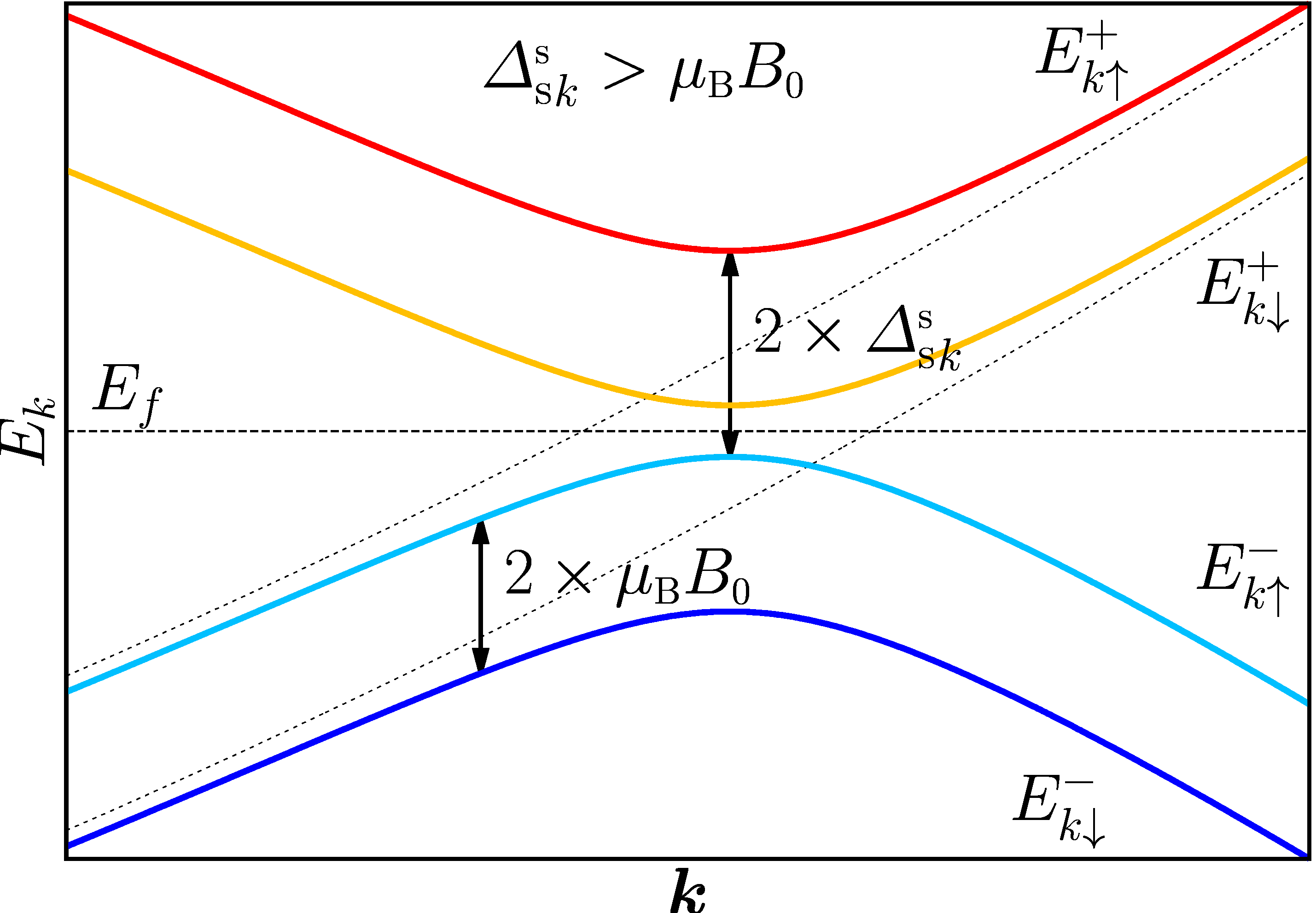
a)

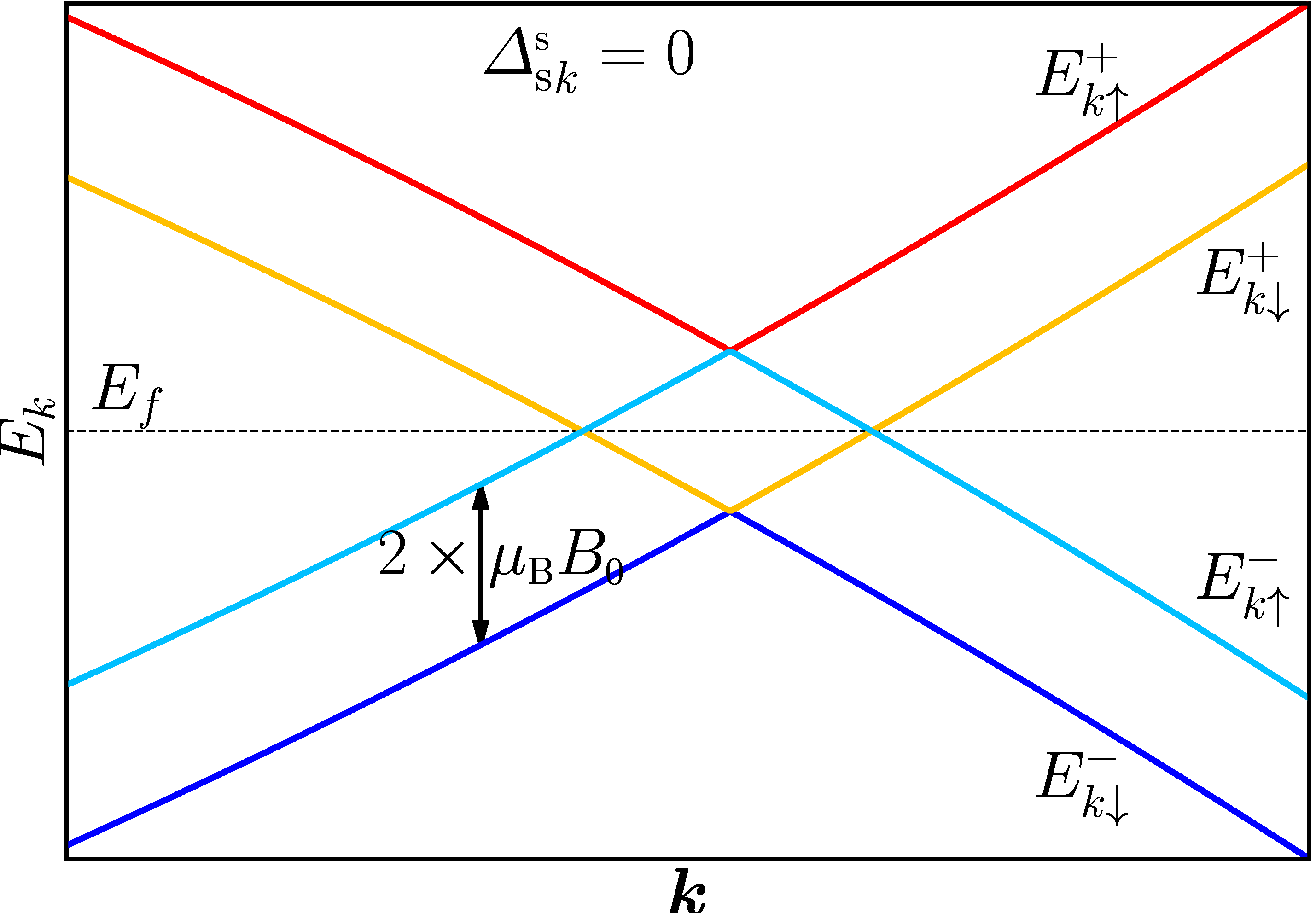
b)

Figure 1: (color online) Sketch of the Bogoliubov eigenvalues $E_{k\sigma}^{\pm}$ for a free electron gas with a homogenous splitting $\varepsilon_{k\sigma}=\frac{1}{2}\boldsymbol{k}^{2}+{\rm sign}(\sigma)\mu_{{\rm{\scriptscriptstyle B}}}B_{{\rm{\scriptscriptstyle 0}}}$. We choose a constant ${\varDelta_{{\rm s}}^{{\scriptscriptstyle{\rm s}}}}_{k}>\mu_{{\rm{\scriptscriptstyle B}}}B_{{\rm{\scriptscriptstyle 0}}}$ in a) and ${\varDelta_{{\rm s}}^{{\scriptscriptstyle{\rm s}}}}_{k}=0$ in b). We plot the $+$ Bogoliubov branch in red and orange for$\uparrow$and $\downarrow$ and the - branch in light blue and dark blue for $\uparrow$and $\downarrow$, respectively. We indicate the $\varepsilon_{k\sigma}$ in a) as thin dashed lines. In a), the $+$ branches are strictly larger than the Fermi Energy $E_{f}$ and thus constitute the SC KS particle excitations. On the other hand for ${\varDelta_{{\rm s}}^{{\scriptscriptstyle{\rm s}}}}_{k}<\mu_{{\rm{\scriptscriptstyle B}}}B_{{\rm{\scriptscriptstyle 0}}}$ as in b), the $+$ and $-$ branch partly swap their order. When $E_{k\uparrow}^{-}>E_{f}$ the SC KS particle excitations are from the $-$ branch also.

In the next paragraph we give a more detailed discussion of the Bogoliubov eigenvalues $E_{k\sigma}^{\pm}$.

Eigenvalues in the SDA

Our first concern is how to interpret the spin quantum number $\sigma$ of $E_{k\sigma}^{\pm}$ in connection with the underlying normal states $\varepsilon_{k\sigma}$.

First, consider the non-SC limit where

$${\varDelta_{{\rm s}}^{{\scriptscriptstyle{\rm s}}}}_{k}=0:\,2E_{k\sigma}^{\pm} = \varepsilon_{k\sigma}-\varepsilon_{-k-\sigma}\pm|\varepsilon_{k\sigma}+\varepsilon_{-k-\sigma}|\,.$$ (86)

This situation is plotted in Fig. 1 b). Note that if $\varepsilon_{k\sigma}+\varepsilon_{-k-\sigma}>0$, than $E_{k\sigma}^{-}=-\varepsilon_{-k-\sigma}$ and if $\varepsilon_{k\sigma}+\varepsilon_{-k-\sigma}<0$ we conclude $E_{k\sigma}^{-}=\varepsilon_{k\sigma}$.

Second, consider the following case that occurs at any $k_{0}$ where $\varepsilon_{k_{0}\uparrow}+\varepsilon_{-k_{0}\downarrow}=0$. Given that we have an energy splitting $\varepsilon_{k_{0}\uparrow}-\varepsilon_{-k_{0}\downarrow}>2|{\varDelta_{{\rm s}}^{{\scriptscriptstyle{\rm s}}}}_{k}|$ we find that both $E_{-k_{0},\downarrow}^{\pm}$ are negative. This means that according to the definition in Eq. (17) to take the positive eigenvalues, both KS particles are from the $\sigma=\uparrow$ branch. It is not possible to construct the Bogoliubov transformations in this case and in any case the $\hat{\gamma}_{k\uparrow}^{\dagger}$ state cannot be occupied twice. It is, however, possible to give up the requirement that all SC KS particles are positive and simply always take the $+$ branch. Then we can say that $\hat{\gamma}_{k\sigma}^{\dagger}$ creates a negative energy excitation which will be occupied in the ground state. By analogy with BCS, $\hat{\gamma}_{k\sigma}^{\dagger}$ creates an electron like single particle state on the SC vacuum, this leads to the interpretation that, in the ground state, this $k$ space region is occupied by unpaired electrons. A similar discussion can be found (still in the context of BCS theory) in the work of SarmaSarma . Similar to Eq. (17) we can redefine electron to hole operators at the price of changing the ground state energy. Because the ground state energy, in turn, cancels from the thermal averages, the expectation values computed with this theory do not depend on this interpretation. We want to point out that this discussion only applies when the splitting is larger than the pair potential.

Eigenvectors in the SDA

Furthermore we can analytically compute the normalized eigenvectors $g_{k\mu}^{\alpha}$ to the eigenvalues $E_{k\mu}^{\alpha}$ ($\alpha=\pm$). We introduce the notation

$$g_{k\sigma}^{\alpha}=\left(\begin{array}[]{c}u_{k\sigma}^{k\alpha}\\ v_{k-\sigma}^{-k\alpha}\end{array}\right)$$ (87)

to label the components which are given in terms of the eigenvalues and components of the matrix by

$$v_{k-\sigma}^{-k\alpha} = \sqrt{\frac{|E_{k\mu}^{\alpha}-\varepsilon_{k\sigma}|}{|E_{k\sigma}^{+}+E_{-k-\sigma}^{+}|}}\,,$$ (88)

$$u_{k\sigma}^{k\alpha} = \frac{\text{sign}(\sigma)}{\text{sign}(\alpha)}\frac{{\varDelta_{{\rm s}}^{{\scriptscriptstyle{\rm s}}}}_{k}}{|{\varDelta_{{\rm s}}^{{\scriptscriptstyle{\rm s}}}}_{k}|}\sqrt{\frac{|\varepsilon_{-k-\sigma}+E_{k\sigma}^{\alpha}|}{|E_{k\sigma}^{\alpha}+E_{-k-\sigma}^{\alpha}|}}\,.$$ (89)

Starting from a converged zero temperature normal state calculation, within the SDA the only remaining variable is thus the matrix elements of the pair potential ${\varDelta_{{\rm s}}^{{\scriptscriptstyle{\rm s}}}}_{k}$ because the SC KS wavefunctions as well as the Bogoliubov eigenvalues are explicitly given in terms of it.

It is important to point out that within the SDA ${\varDelta_{{\rm s}}^{{\scriptscriptstyle{\rm s}}}}_{k}$ can be chosen to be realNambu (1960); Anderson (1958). This can be proved by exploiting the gauge symmetry of Eq. (83) under rotation about the $\tau_{z}$ axis. If the rotation is applied with a $k$ dependent angle $\theta_{k}$ of

$$\theta_{k}=\text{arctan}\Bigl{(}\frac{\Im{\varDelta_{{\rm s}}^{{\scriptscriptstyle{\rm s}}}}_{k}}{\Re{\varDelta_{{\rm s}}^{{\scriptscriptstyle{\rm s}}}}_{k}}\Bigr{)}$$ (90)

we get:

$$\text{e}^{-\text{i}\tau_{z}\frac{\theta_{k}}{2}}\left(\begin{array}[]{cc}\varepsilon_{k\sigma}&{\rm sign}(\sigma){\varDelta_{{\rm s}}^{{\scriptscriptstyle{\rm s}}}}_{k}\\ {\rm sign}(\sigma){\varDelta_{{\rm s}}^{{\scriptscriptstyle{\rm s}}}}_{k}^{\ast}&-\varepsilon_{-k-\sigma}\end{array}\right)\text{e}^{\text{i}\tau_{z}\frac{\theta_{k}}{2}}$$ (93)

$$= \left(\begin{array}[]{cc}\varepsilon_{k\sigma}&{\rm sign}(\sigma){\tilde{\varDelta_{{\rm s}}^{{\scriptscriptstyle{\rm s}}}}}_{k}\\ {\rm sign}(\sigma){\tilde{\varDelta_{{\rm s}}^{{\scriptscriptstyle{\rm s}}}}}_{k}&-\varepsilon_{-k-\sigma}\end{array}\right)$$ (96)

where ${\tilde{\varDelta_{{\rm s}}^{{\scriptscriptstyle{\rm s}}}}}_{k}={\rm sign}(\Re{\varDelta_{{\rm s}}^{{\scriptscriptstyle{\rm s}}}}_{k})|{\varDelta_{{\rm s}}^{{\scriptscriptstyle{\rm s}}}}_{k}|\in\mathbb{R}$. Thus the $(k,-k)$ matrix elements of our general complex decoupled pair potential are gauge equivalent to purely real ones. We still keep a general complex notation for ${\varDelta_{{\rm s}}^{{\scriptscriptstyle{\rm s}}}}_{k}$ first, to investigate explicitly if self-energy corrections affect this conclusion and, second, to make it easier to extent the formalism to the case where the gauge symmetry does not have enough freedom to make all matrix elements real.

III.1.3 Competition between SC and Magnetism in the SDA

The SDA, as introduced so far, assumes that we compute SC on top of a (magnetic) quasi particle structure. Thus, for example, it does not allow magnetism to be suppressed when a weakly magnetic system becomes SC. In conventional SCDFT Lüders et al. (2005); Marques et al. (2005) this type of feedbacks can be safely neglected because SC changes the dispersion only for states very close to the Fermi level. The effect on the electronic density is thus negligible and so is the change in the normal state $xc$ potential. However, since the contributions to $\boldsymbol{m}(\boldsymbol{r})$ are in general more localized at the Fermi level, assuming quasi particle energies $\varepsilon_{i\sigma}$ to be unaffected when SC sets in may not be reasonable for magnetic systems.

We want to point out in here that it is also possible to keep the simple form of the SDA and include competition of SC and magnetism at the same time, by means of the following iterative scheme:

1. Take the normal KS states $\{\vec{\varphi}_{i\sigma}\}$ and eigenvalues $\varepsilon_{k\sigma}$ as starting orbitals.

2. Solve the KS-BdG equations in the SDA

3. Recompute the densities $n(\boldsymbol{r})$ and $\boldsymbol{m}(\boldsymbol{r})$ according to the Eqs. (56) and (57)

4. Re-diagonalize the normal state KS equations with the updated densities (in particular changes in $\boldsymbol{m}(\boldsymbol{r})$ may be of relevance)

5. iterate from point 2. until self consistence is reached

This procedure changes the meaning of the SDA during the iteration because we are self consistently updating the orbitals $\{\vec{\varphi}_{i\sigma}\}$ it refers to.

III.2 The Sham-Schlüter Equation of SpinSCDFT

So far we have presented the structure of SpinSCDFT with the focus on the electronic SC KS system. However explicit functionals for the $xc$-pairing potential ${\varDelta_{{\rm s}}^{{\scriptscriptstyle{\rm s}}}}_{k}$ have not yet been discussed. The derivation of the approximations for the $xc$-potentials generalizes one proposed by MarquesMarques (2000) in SCDFT and uses the Sham-Schlüter equation of SpinSCDFT. This equation is based on the observation that the parts of the KS GF and the interaction GF that correspond to the densities must be equal. Using the Dyson equation for a SC in a magnetic field starting from the SC KS system as the formally non interaction one we can relate the $xc$-potentials to an approximation for the self energy. Here and in the next section we present a derivation of an $xc$-potential for SpinSCDFT that generalizes the ones of MarquesMarques (2000) and Sanna and GrossSanna and Gross .

We introduce the GF with the $\tau$ ordering symbol $\bar{{\rm T}}$ and the field operators in the Heisenberg picture

$$\bar{G}(\boldsymbol{r}\tau,\boldsymbol{r}^{\prime}\tau^{\prime})=-\langle\bar{{\rm T}}\hat{\varPsi}(\boldsymbol{r}\tau)\otimes\hat{\varPsi}^{\dagger}(\boldsymbol{r}^{\prime}\tau^{\prime})\rangle\,.$$ (97)

The imaginary time ordering symbol in Nambu space $\bar{{\rm T}}$ is defined to act on every of the $(4\times 4)$ components individually which can be achieved by transposing in Nambu-spin space

$$\bar{{\rm T}}\hat{\varPsi}(\boldsymbol{r}\tau)\!\otimes\!\hat{\varPsi}^{\dagger}(\boldsymbol{r}^{\prime}\tau^{\prime}) = \uptheta(\tau\!-\!\tau^{\prime})\hat{\varPsi}(\boldsymbol{r}\tau)\!\otimes\!\hat{\varPsi}^{\dagger}(\boldsymbol{r}^{\prime}\tau^{\prime})$$ (98)

$$-\uptheta(\tau^{\prime}\!\!-\!\tau)\bigl{(}\hat{\varPsi}^{\dagger}(\boldsymbol{r}^{\prime}\tau^{\prime})\!\otimes\!\hat{\varPsi}(\boldsymbol{r}\tau)\bigr{)}^{{\rm T}_{\text{sn}}}\,.$$

We define the equal time limit in the $-1,-1$ component different to the usual one (that we use in the $1,1$ component). The equal time limit of the time ordering symbol should be defined to recover the density matrix operator but according to the usual rule where the creation operator is taken infinitesimally before the annihilator would lead to the form $\psi\psi^{\dagger}$ in the $-1,-1$ component. From the equation of motion we derive the Dyson equation starting from the SC KS system as a formally non interacting system

$$\bar{G}(\boldsymbol{r},\boldsymbol{r}^{\prime},\omega_{n})=\bar{G}^{{\scriptscriptstyle{\rm KS}}}(\boldsymbol{r},\boldsymbol{r}^{\prime},\omega_{n})+$$

$$\int{\rm d}\boldsymbol{r}_{1}\!\int{\rm d}\boldsymbol{r}_{1}^{\prime}\bar{G}^{{\scriptscriptstyle{\rm KS}}}\!(\boldsymbol{r}\!,\!\boldsymbol{r}_{1}\!,\!\omega_{n})\!\cdot\!\bar{\varSigma}^{{\scriptscriptstyle{\rm s}}}(\boldsymbol{r}_{1}\!,\!\boldsymbol{r}_{1}^{\prime}\!,\!\omega_{n})\!\cdot\!\bar{G}(\boldsymbol{r}_{1}^{\prime}\!,\!\boldsymbol{r}^{\prime}\!\!,\omega_{n}),$$

(99)

with

$$\bar{\varSigma}^{{\scriptscriptstyle{\rm s}}}(\boldsymbol{r},\boldsymbol{r}^{\prime},\omega_{n})=\bar{\varSigma}(\boldsymbol{r},\boldsymbol{r}^{\prime},\omega_{n})\!-\bar{v}_{{\scriptscriptstyle{\rm xc}}}(\boldsymbol{r},\boldsymbol{r}^{\prime})\,.$$ (100)

Here $\bar{\varSigma}$ is the irreducible Nambu self-energy, where the electronic Hartree diagram was subtracted, and $\bar{v}_{{\scriptscriptstyle\text{xc}}}$ is the Nambu $xc$ potential

$$\bar{v}_{{\scriptscriptstyle{\rm xc}}}(\boldsymbol{r}\!,\!\boldsymbol{r}^{\prime})=$$

$$\left(\!\begin{array}[]{cc}\updelta(\boldsymbol{r}\!-\!\boldsymbol{r}^{\prime})\bigl{(}\sigma_{0}v_{{\scriptscriptstyle{\rm xc}}}(\boldsymbol{r})\!-\!\mathbf{S}\!\cdot\!\boldsymbol{B}_{{\scriptscriptstyle{\rm xc}}}(\boldsymbol{r})\bigr{)}&\boldsymbol{\Phi}\cdot\boldsymbol{\varDelta}^{{\scriptscriptstyle{\rm xc}}}(\boldsymbol{r}\!,\!\boldsymbol{r}^{\prime})\\ -\boldsymbol{\Phi}\cdot\boldsymbol{\varDelta}^{{\scriptscriptstyle{\rm xc}}\ast}(\boldsymbol{r}\!,\!\boldsymbol{r}^{\prime})&-\updelta(\boldsymbol{r}\!-\!\boldsymbol{r}^{\prime})\bigl{(}\sigma_{0}v_{{\scriptscriptstyle{\rm xc}}}(\boldsymbol{r})\!-\!\mathbf{S}^{\ast}\!\!\cdot\!\boldsymbol{B}_{{\scriptscriptstyle{\rm xc}}}(\boldsymbol{r})\bigr{)}\end{array}\!\right)$$ (103)

(104)

The SC KS Greens function satisfies

$$\int{\rm d}\boldsymbol{r}_{1}\Bigl{(}{\rm i}\omega_{n}\updelta(\boldsymbol{r}-\boldsymbol{r}_{1})\tau_{0}\sigma_{0}-\bar{H}_{{\scriptscriptstyle{\rm KS}}}(\boldsymbol{r}\!,\!\boldsymbol{r}_{1})\Bigr{)}\!\!\cdot\!\bar{G}^{{\scriptscriptstyle{\rm KS}}}(\boldsymbol{r}_{1},\boldsymbol{r}^{\prime}\!,\omega_{n})$$

$$\qquad=\updelta(\boldsymbol{r}-\boldsymbol{r}^{\prime})\tau_{0}\sigma_{0}\,.$$ (105)

From the equation of motion we can compute the SC KS GF. Because by construction the SC KS GF yields the same densities as the interacting system we can cancel the respective parts of the GFs in the Dyson Eq. (99) that correspond to the densities. The result is the Sham-Schlüter equation

$$\frac{1}{\beta}\sum_{n}\int{\rm d}\boldsymbol{r}_{1}\int{\rm d}\boldsymbol{r}_{1}^{\prime}\Bigl{[}\bar{G}^{{\scriptscriptstyle{\rm KS}}}(\boldsymbol{r},\boldsymbol{r}_{1},\omega_{n})\cdot$$

$$\cdot\bar{\varSigma}^{{\scriptscriptstyle{\rm s}}}(\boldsymbol{r}_{1},\boldsymbol{r}_{1}^{\prime},\omega_{n})\cdot\bar{G}(\boldsymbol{r}_{1}^{\prime}\!,\boldsymbol{r}^{\prime}\!\!,\omega_{n})\Bigr{]}_{\alpha,-\alpha}=0$$ (106)

$$\frac{1}{\beta}\sum_{n}\int{\rm d}\boldsymbol{r}_{1}\int{\rm d}\boldsymbol{r}_{1}^{\prime}\Bigl{[}\bar{G}^{{\scriptscriptstyle{\rm KS}}}(\boldsymbol{r},\boldsymbol{r}_{1},\omega_{n})\cdot$$

$$\cdot\bar{\varSigma}^{{\scriptscriptstyle{\rm s}}}(\boldsymbol{r}_{1},\boldsymbol{r}_{1}^{\prime},\omega_{n})\cdot\bar{G}(\boldsymbol{r}_{1}^{\prime}\!,\boldsymbol{r}\!\!,\omega_{n})\Bigr{]}_{\alpha,\alpha}=0\,.$$ (107)

For convenience the self energy is decomposed in a phononic part $\bar{\varSigma}_{{\scriptscriptstyle{\rm ph}}}(\omega_{n})$ and a Coulomb part $\bar{\varSigma}_{{\scriptscriptstyle{\rm C}}}(\omega_{n})$ :

$$\bar{\varSigma}(\omega_{n})=\bar{\varSigma}_{{\scriptscriptstyle{\rm ph}}}(\omega_{n})+\bar{\varSigma}_{{\scriptscriptstyle{\rm C}}}(\omega_{n})\,.$$ (108)

$\bar{\varSigma}(\omega_{n})$ has a diagrammatic expansion in terms of $\bar{G}(\omega_{n})$ Vonsovsky et al. (1982) and can be even viewed as part of a Hedin cycle for a SC including phononic and Coulomb interactions Linscheid and Essenberger . We do not consider vertex corrections, thus the Coulomb self energy part $\bar{\varSigma}_{{\scriptscriptstyle{\rm C}}}$ is the electronic GW diagram
$\bar{\varSigma}_{{\scriptscriptstyle{\rm C}}}(\omega_{n})\approx$ . (109)

As an interesting extension we could include parts of the vertex corrections that lead to spin fluctuations. These, in the form of an effective spin interaction, are discussed by Essenberger et al.Essenberger et al. and the extension to the present spin dependent formalism is straightforward. As compared to the polarization corrections of the same order, the phononic vertex corrections are negligible Migdal (1958).

Moreover due to the quality of the phonon spectra one obtains with density functional perturbation theory Baroni et al. (2001); Giannozzi et al. (1991) we do not consider further diagrammatic electronic screening and treat the phononic interaction in the Hartree-Fock approximation
$\bar{\varSigma}_{{\scriptscriptstyle{\rm ph}}}(\omega_{n})\approx$$+$ . (110)

It has been observed that computing the GW quasi particle band structure in a metal gives usually small corrections to the KS bands (compare Ref. Marini et al., 2001 Fig. 2), also densities result to be almost identical. Thus, at least in the spin degenerate case, the GW corrections on a KS band structure of a metal are usually neglected. For convenience we use a similar assumption for the spin part. This way we can drop the Nambu diagonal $\bar{v}_{{\scriptscriptstyle{\rm xc}}}$ construction from the Sham-Schlüter equation. Representing $\bar{G}^{{\scriptscriptstyle{\rm KS}}}(\boldsymbol{r},\boldsymbol{r}^{\prime},\omega_{n})$ and $\bar{G}(\boldsymbol{r},\boldsymbol{r}^{\prime},\omega_{n})$ in the same basis as the Bogoliubov-Valatin transformations, i.e. essentially the normal state KS orbitals $\{\varPsi_{i\sigma\alpha}^{{\scriptscriptstyle{\rm KS}}}(\boldsymbol{r})\}$ with the pure Nambu and spin spinor wavefunctions

$$\varPsi_{i\sigma\alpha}^{{\scriptscriptstyle{\rm KS}}}(\boldsymbol{r})=\left(\begin{array}[]{c}\updelta_{\alpha,1}\vec{\varphi}_{i\sigma}(\boldsymbol{r})\\ \updelta_{\alpha,-1}\vec{\varphi}_{i\sigma}^{\ast}(\boldsymbol{r})\end{array}\right)\,.$$ (111)

Sorting the expansion coefficients of $\bar{G}^{{\scriptscriptstyle{\rm KS}}}(\boldsymbol{r},\boldsymbol{r}^{\prime},\omega_{n})=\sum_{\alpha\alpha^{\prime}\sigma\sigma^{\prime}ij}\bar{G}_{i\alpha\sigma j\alpha^{\prime}\sigma^{\prime}}^{{\scriptscriptstyle{\rm KS}}}(\omega_{n})\varPsi_{i\alpha\sigma}^{{\scriptscriptstyle{\rm KS}}}(\boldsymbol{r})\otimes\varPsi_{j\alpha^{\prime}\sigma^{\prime}}^{{\scriptscriptstyle{\rm KS}}}(\boldsymbol{r}^{\prime})$ in similar Nambu and spin form we obtain the $4N\times 4N$ matrix equation

$$\frac{1}{\beta}\sum_{n}\bar{G}^{{\scriptscriptstyle{\rm KS}}}(\omega_{n})\cdot\left(\begin{array}[]{cc}0&\boldsymbol{\Phi}\cdot\boldsymbol{\varDelta}^{{\scriptscriptstyle{\rm s}}}\\ (\boldsymbol{\Phi}\cdot\boldsymbol{\varDelta}^{{\scriptscriptstyle{\rm s}}})^{\dagger}&0\end{array}\right)\cdot\bar{G}(\omega_{n})$$ (114)

$$=\frac{1}{\beta}\sum_{n}\bar{G}^{{\scriptscriptstyle{\rm KS}}}(\omega_{n})\cdot\Biggl{(}\biggl{(}\begin{array}[]{cc}0&\bar{\varSigma}_{{\scriptscriptstyle{\rm C}}}^{{\scriptscriptstyle 1,-1}}(\omega_{n})\\ \bar{\varSigma}_{{\scriptscriptstyle{\rm C}}}^{{\scriptscriptstyle-1,1}}(\omega_{n})&0\end{array}\biggr{)}$$ (117)

$$\qquad\qquad\qquad+\bar{\varSigma}_{{\scriptscriptstyle{\rm ph}}}(\omega_{n})\Biggr{)}\cdot\bar{G}(\omega_{n})$$ (118)

that we need to solve for $\boldsymbol{\Phi}\cdot\boldsymbol{\varDelta}^{{\scriptscriptstyle{\rm s}}}$. From here on we use $\boldsymbol{\Phi}\cdot\boldsymbol{\varDelta}^{{\scriptscriptstyle{\rm s}}}$ and $\boldsymbol{\Phi}\cdot\boldsymbol{\varDelta}^{{\scriptscriptstyle{\rm xc}}}$ synonymously, i.e. the external pair potential is assumed to be infinitesimal.

In the next section we reduce the problem to the singlet case and employ the SDA. Because we can solve the KSBdG equations analytically we obtain a potential functional theory and arrive at a functional form that is formally similar to the BCS gap equation. We stress that the methods presented here and in the next section could also be applied without the restriction to the SDA. However in that case the equations would have an implicit form and require a numerical solution of the KSBdG equations. Such a general form would be of importance in considering triplet superconductivity or to account for pairings beyond the usual one of time reversed states (as would be needed for example to describe the FFLO state Fulde and Ferrell (1964); Larkin ). A further discussion can be found in Ref. Linscheid, 2014.

III.3 Derivation $xc-$Potential

The Sham-Schlüter Eq. (118) involves the interacting GF which is usually only available after solving the Dyson equation. In an approximate scheme this step can be avoided. The straightforward way is to replace the matrix $\bar{G}(\omega_{n})$ with $\bar{G}^{{\scriptscriptstyle\text{KS}}}(\omega_{n})$ on all occurrences. As was realized before Lüders et al. (2005) this violates Migdal’s theorem because there the vertex is compared with the polarization diagram of the same order. Thus the phonon vertex corrections are only negligible as compared to the Hartree exchange diagram with the full GF. To circumvent this problem some of the Authors introduced a procedure to construct a self-energy that does satisfy Migdal’s theorem Sanna and Gross . Starting from an electron gas model with a phononic Hartree exchange diagram, this leads to excellent agreement with experiment while still retaining the numerically simple form of the Sham-Schlüter equation that is independent on $\bar{G}(\omega_{n})$ and involves only Matsubara sums that can be evaluated analytically. The self-energy $\bar{\varSigma}^{{\scriptscriptstyle{\rm KS}}}(\omega_{n})$ with $\bar{G}(\omega_{n})$ replaced by $\bar{G}_{ij}^{{\scriptscriptstyle\text{KS}}}(\omega_{n})$ is the basis of all further improvements. In this work, however, we will not investigate the parametrization procedure. We will limit the complexity of the derivation by using assuming $\bar{\varSigma}(\omega_{n})\simeq\bar{\varSigma}^{{\scriptscriptstyle{\rm KS}}}(\omega_{n})$, where in $\bar{\varSigma}^{{\scriptscriptstyle{\rm KS}}}(\omega_{n})$ the $\bar{G}(\omega_{n})$ is replaced by $\bar{G}_{ij}^{{\scriptscriptstyle\text{KS}}}(\omega_{n})$. This will give inaccurate critical temperatures but qualitatively correct results. Thus we are left to solve the equation:

$$\frac{1}{\beta}\sum_{n}\bar{G}^{{\scriptscriptstyle{\rm KS}}}(\omega_{n})\cdot\left(\begin{array}[]{cc}0&\boldsymbol{\Phi}\cdot\boldsymbol{\varDelta}^{{\scriptscriptstyle{\rm s}}}\\ (\boldsymbol{\Phi}\cdot\boldsymbol{\varDelta}^{{\scriptscriptstyle{\rm s}}})^{\dagger}&0\end{array}\right)\cdot\bar{G}^{{\scriptscriptstyle{\rm KS}}}(\omega_{n})$$ (121)

$$=\frac{1}{\beta}\sum_{n}\bar{G}^{{\scriptscriptstyle{\rm KS}}}(\omega_{n})\cdot\Biggl{(}\biggl{(}\begin{array}[]{cc}0&\bar{\varSigma}_{{\scriptscriptstyle{\rm C}}}^{{\scriptscriptstyle{\rm KS}}{\scriptscriptstyle 1,-1}}(\omega_{n})\\ \bar{\varSigma}_{{\scriptscriptstyle{\rm C}}}^{{\scriptscriptstyle{\rm KS}}{\scriptscriptstyle-1,1}}(\omega_{n})&0\end{array}\biggr{)}$$ (124)

$$\qquad\qquad\qquad+\bar{\varSigma}_{{\scriptscriptstyle{\rm ph}}}^{{\scriptscriptstyle{\rm KS}}}(\omega_{n})\Biggr{)}\cdot\bar{G}^{{\scriptscriptstyle{\rm KS}}}(\omega_{n})\,.$$ (125)

In this form the matrix elements of the SC KS GF in the normal state KS basis are given by

$$\bar{G}_{ij}^{{\scriptscriptstyle{\rm KS}}}(\omega_{n}) = \sum_{k}\frac{1}{\mbox{i}\omega_{n}-E_{k}}\left(\begin{array}[]{cc}\vec{u}_{k}^{i}\otimes\vec{u}_{k}^{j\ast}&\vec{u}_{k}^{i}\otimes\vec{v}_{k}^{j\ast}\\ \vec{v}_{k}^{i}\otimes\vec{u}_{k}^{j\ast}&\vec{v}_{k}^{i}\otimes\vec{v}_{k}^{j\ast}\end{array}\right)+$$ (131)

$$+\sum_{k}\frac{1}{\mbox{i}\omega_{n}+E_{k}}\left(\begin{array}[]{cc}\vec{v}_{k}^{i\ast}\otimes\vec{v}_{k}^{j}&\vec{v}_{k}^{i\ast}\otimes\vec{u}_{k}^{j}\\ \vec{u}_{k}^{i\ast}\otimes\vec{v}_{k}^{j}&\vec{u}_{k}^{i\ast}\otimes\vec{u}_{k}^{j}\end{array}\right)\,.$$

We use $\vec{u}_{k}^{i}=(\begin{array}[]{cc}u_{k}^{i\uparrow}&u_{k}^{i\downarrow})^{{\rm T}}\end{array}$ with the expansion coefficients $u_{k}^{i\sigma}$ of $\vec{u}_{k}(\mathbf{r})$ in $\vec{\varphi}_{i\sigma}(\mathbf{r})$ given in Eq. (45). Similar for $\vec{v}_{k}^{i}$. Further we assume the SDA for the rest of this paper. Results beyond the SDA are discussed in the PhD thesis Ref. Linscheid, 2014. In the SDA the SC KS GF simplifies to

$$\bar{G}_{ij}^{{\scriptscriptstyle\text{KS}}}(\omega_{n})\!=$$

$$\sum_{\alpha}\!\!\left(\begin{array}[]{cccc}\frac{|u_{i\uparrow}^{i\alpha}|^{2}\delta_{ij}}{\mbox{i}\omega_{n}-E_{i\uparrow}^{\alpha}}&0&0&\frac{u_{i\uparrow}^{i\alpha}(v_{i\downarrow}^{-i\alpha})^{\ast}\delta_{i,-j}}{\mbox{i}\omega_{n}-E_{i\uparrow}^{\alpha}}\\ 0&\frac{|u_{i\downarrow}^{i\alpha}|^{2}\delta_{ij}}{\mbox{i}\omega_{n}-E_{i\downarrow}^{\alpha}}&\frac{u_{i\downarrow}^{i\alpha}(v_{i\uparrow}^{-i\alpha})^{\ast}\delta_{i,-j}}{\mbox{i}\omega_{n}-E_{i\downarrow}^{\alpha}}&0\\ 0&\frac{(u_{i\uparrow}^{i\alpha})^{\ast}v_{i\downarrow}^{-i\alpha}\delta_{i,-j}}{\mbox{i}\omega_{n}+E_{i\uparrow}^{\alpha}}&\frac{|u_{i\uparrow}^{i\alpha}|^{2}\delta_{ij}}{\mbox{i}\omega_{n}+E_{i\uparrow}^{\alpha}}&0\\ \frac{(u_{i\downarrow}^{i\alpha})^{\ast}v_{i\uparrow}^{-i\alpha}\delta_{i,-j}}{\mbox{i}\omega_{n}+E_{i\downarrow}^{\alpha}}&0&0&\frac{|u_{i\downarrow}^{i\alpha}|^{2}\delta_{ij}}{\mbox{i}\omega_{n}+E_{i\downarrow}^{\alpha}}\end{array}\right)$$ (136)

(137)

This form and any further formula based on it use the components of the SC KS wavefunction as given in the Eqs. (88) and (89). In the Dyson equation $\bar{G}^{-1}={\mbox{$\bar{G}^{{\scriptscriptstyle\text{KS}}}$}}^{-1}-\bar{\varSigma}$ we see that we need to compare the self-energy contributions with the inverse SC KS GF. Inverting $\bar{G}_{ij}^{{\scriptscriptstyle\text{KS}}}(\omega_{n})$ with obtain

$$(\bar{G}^{{\scriptscriptstyle\text{KS}}})_{ij}^{-1}(\omega_{n}) = \delta_{ij}\Bigl{(}\text{i}\omega_{n}\tau_{0}\sigma_{0}-\bigl{(}\frac{\varepsilon_{i\uparrow}+\varepsilon_{-i\downarrow}}{2}\bigr{)}\tau_{z}\sigma_{0}$$ (138)

$$-\bigl{(}\frac{\varepsilon_{i\uparrow}-\varepsilon_{-i\downarrow}}{2}\bigr{)}\tau_{z}\sigma_{z}\Bigr{)}+\delta_{i,-j}\bigl{(}(\mbox{i}\tau_{y})(\mbox{i}\sigma_{y})\Re{\varDelta_{{\rm s}}^{{\scriptscriptstyle{\rm s}}}}_{i}$$

$$+\tau_{x}(\mbox{i}\sigma_{y})\mbox{i}\Im{\varDelta_{{\rm s}}^{{\scriptscriptstyle{\rm s}}}}_{i}\bigr{)}\,.$$

Here we see that self-energy contributions $\propto\tau_{z}\sigma_{0}$ change the average spin Fermi level $\frac{\varepsilon_{i\uparrow}+\varepsilon_{-i\downarrow}}{2}=0$. Similarly contributions $\propto\tau_{z}\sigma_{z}$ change the splitting of single particle levels. It has to be understood that these are global properties of the band structure, meaning that the full $\varepsilon_{i\sigma}$ dispersion has to be integrated to obtain $N$ electrons per unit cell. If the interaction changes dispersion and occupations far away from the Fermi level this may still cause a shift of the original Fermi level. An clear cut example is the following: In the context of SC one often employs the Eliashberg function $\alpha^{\!2}\!F(\varOmega)$ which is the Fermi-surface average of the electron-phonon interaction Eliashberg (1960); Allen and Mitrović (1983); Carbotte (1990), to describe the electron phonon interaction. This function is assumed to apply equally to all states, also those away from the Fermi level. This is a good approximation only if corrections of the Fermi level are excluded a priori (electron-hole symmetry), otherwise under this assumption the correction to the Fermi level $\frac{\varepsilon_{i\uparrow}+\varepsilon_{-i\downarrow}}{2}$ and the splitting $\frac{\varepsilon_{i\uparrow}-\varepsilon_{-i\downarrow}}{2}$ would show a logaritmic divergece. As commonly done in Eliashberg theory, where the same effect occurs, one then excludes self-energy contributions $\propto\tau_{z}$. We will assume the same approximation. As the Hartree diagram is proportional to $\tau_{z}$ is thus not considered. While the expected Fermi energy shift is negligible, corrections to the spin splitting $\frac{\varepsilon_{i\uparrow}-\varepsilon_{-i\downarrow}}{2}$ could be of relevance. However due to the extreme additional numerical complexity of considering the true full electronic state dependence of the electron phonon interaction we leave this to a future project. We compute the self-energy matrix elements in the SDA from the Eq. (110)

$${\mbox{$\bar{\varSigma}_{{\scriptscriptstyle{\rm ph}}}^{{\scriptscriptstyle{\rm KS}}}$}}_{i\sigma j\sigma^{\prime}}^{{\scriptscriptstyle 1,1}}(\omega_{n})=\updelta_{\sigma\sigma^{\prime}}\sum_{qk\alpha}g_{ik\sigma}^{q}g_{kj\sigma}^{-q}\times$$

$$\times|u_{k\sigma}^{k\alpha}|^{2}M_{{\scriptscriptstyle{\rm ph}}}(\varOmega_{q},E_{k\sigma}^{\alpha},\omega_{n})$$ (139)

$${\mbox{$\bar{\varSigma}_{{\scriptscriptstyle{\rm ph}}}^{{\scriptscriptstyle{\rm KS}}}$}}_{i\sigma j\sigma^{\prime}}^{{\scriptscriptstyle 1,-1}}(\omega_{n})=-\updelta_{\sigma,-\sigma^{\prime}}\sum_{qk\alpha}g_{ik\sigma}^{q}g_{j,-k,-\sigma}^{-q}\times$$

$$\times u_{k\sigma}^{k\alpha}(v_{k-\sigma}^{-k\alpha})^{\ast}M_{{\scriptscriptstyle{\rm ph}}}(\varOmega_{q},E_{k\sigma}^{\alpha},\omega_{n})$$ (140)

$${\mbox{$\bar{\varSigma}_{{\scriptscriptstyle{\rm ph}}}^{{\scriptscriptstyle{\rm KS}}}$}}_{i\sigma j\sigma^{\prime}}^{{\scriptscriptstyle-1,1}}(\omega_{n})=-\updelta_{\sigma,-\sigma^{\prime}}\sum_{qk\alpha}g_{ki\sigma}^{q}g_{-k,j,-\sigma}^{-q}\times$$

$$\times(u_{k\sigma}^{k\alpha})^{\ast}v_{k-\sigma}^{-k\alpha}M_{{\scriptscriptstyle{\rm ph}}}(\varOmega_{q},-E_{k\sigma}^{\alpha},\omega_{n})$$ (141)

$${\mbox{$\bar{\varSigma}_{{\scriptscriptstyle{\rm ph}}}^{{\scriptscriptstyle{\rm KS}}}$}}_{i\sigma j\sigma^{\prime}}^{{\scriptscriptstyle-1,-1}}(\omega_{n})=\updelta_{\sigma\sigma^{\prime}}\sum_{ak\alpha}g_{ki\sigma}^{q}g_{jk\sigma}^{-q}\times$$

$$\times|u_{k\sigma}^{k\alpha}|^{2}M_{{\scriptscriptstyle{\rm ph}}}(\varOmega_{q},-E_{k\sigma}^{\alpha},\omega_{n})\,.$$ (142)

From the hermiticity of $\hat{H}_{{\scriptscriptstyle{\rm KS}}}^{{\scriptscriptstyle{\rm e-ph}}}$ of Eq. (14) comes $g_{-q}^{a}(\boldsymbol{r})=\bigl{(}g_{q}^{a}(\boldsymbol{r})\bigr{)}^{\ast}$ and thus the electron phonon interaction matrix elements

$$g_{ij\sigma}^{q}=\int{\rm d}\boldsymbol{r}\sum_{a=0,z}\vec{\varphi}_{i\sigma}^{\ast}(\boldsymbol{r})\cdot\sigma_{a}\cdot\vec{\varphi}_{j\sigma}(\boldsymbol{r})g_{q}^{a}(\boldsymbol{r})$$ (143)

have the property $g_{ij\sigma}^{q}={g_{ji\sigma}^{-q}}^{\ast}$. Moreover $g_{ij\sigma}^{q}\propto\updelta_{\boldsymbol{k}_{i},\boldsymbol{k}_{j}+\boldsymbol{q}}$ which is expected from the lattice translational symmetry Baroni et al. (2001). The Matsubara summation $M_{{\scriptscriptstyle{\rm ph}}}(\varOmega,E,\omega_{n})$ is evaluated with the result

$$Y_{{\scriptscriptstyle{\rm ph}}}(\varOmega,E,\omega_{n}) = \frac{1}{\beta}\sum_{n^{\prime}}\frac{1}{\text{i}\omega_{n^{\prime}}-E}\frac{1}{\mbox{i}(\omega_{n}-\omega_{n^{\prime}})+\varOmega}$$ (144)

$$= \frac{n_{\beta}(\varOmega)+f_{\beta}(E)}{\varOmega-E+\text{i}\omega_{n}}$$ (145)

$$M_{{\scriptscriptstyle{\rm ph}}}(\varOmega,E,\omega_{n}) = \frac{n_{\beta}(\varOmega)+f_{\beta}(E)}{\varOmega-E+\text{i}\omega_{n}}+\frac{f_{\beta}(E)+n_{\beta}(-\varOmega)}{\varOmega+E-\text{i}\omega_{n}}$$ (147)

$$= Y_{{\scriptscriptstyle{\rm ph}}}(\varOmega,E,\omega_{n})\!-\!Y_{{\scriptscriptstyle{\rm ph}}}^{\ast}(\varOmega,-E,\omega_{n})\,,$$

where $f_{\beta}(E)$ and $n_{\beta}(\varOmega)$ are Fermi and Bose functions, respectively. The Coulomb self energy parts on the Nambu off diagonal with the diagram of Eq. (109) are

$${\mbox{$\bar{\varSigma}_{{\scriptscriptstyle{\rm C}}}^{{\scriptscriptstyle{\rm KS}}}$}}_{\,i\sigma j\sigma^{\prime}}^{\!{\scriptscriptstyle 1,-1}}(\omega_{n})=-\updelta_{\sigma,-\sigma^{\prime}}\sum_{k\alpha}{W_{ikj,-k}^{{\scriptscriptstyle\text{stat}}}}_{\sigma,-\sigma}\times$$

$$\times u_{k\sigma}^{k\alpha}v_{k-\sigma}^{-k\alpha\ast}f_{\beta}(E_{k\sigma}^{\alpha})\,,$$ (148)

$${\mbox{$\bar{\varSigma}_{{\scriptscriptstyle{\rm C}}}^{{\scriptscriptstyle{\rm KS}}}$}}_{\,i\sigma j\sigma^{\prime}}^{\!{\scriptscriptstyle-1,1}}(\omega_{n})=-\updelta_{\sigma,-\sigma^{\prime}}\sum_{k\alpha}{W_{ki,-k,j}^{{\scriptscriptstyle\text{stat}}}}_{\sigma,-\sigma}\times$$

$$\times u_{k\sigma}^{k\alpha\ast}v_{k-\sigma}^{-k\alpha}f_{\beta}(\!-\!E_{k\sigma}^{\alpha}\!)\,.$$ (149)

with the static screened Coulomb matrix elements

$${W_{k_{1}k_{2}k_{3}k_{4}}^{{\scriptscriptstyle\text{stat}}}}_{\sigma\sigma^{\prime}} = \int{\rm d}\boldsymbol{r}\int{\rm d}\boldsymbol{r}^{\prime}\vec{\varphi}_{k_{1}\sigma}^{\ast}(\boldsymbol{r})\cdot\vec{\varphi}_{k_{2}\sigma}(\boldsymbol{r})\times$$ (150)

$$\times\frac{\epsilon^{-1}(\boldsymbol{r},\boldsymbol{r}^{\prime},0)}{|\boldsymbol{r}-\boldsymbol{r}^{\prime}|}\vec{\varphi}_{k_{3}\sigma^{\prime}}^{\ast}(\boldsymbol{r}^{\prime})\cdot\vec{\varphi}_{k_{4}\sigma^{\prime}}(\boldsymbol{r}^{\prime})\,,$$

with the inverse dielectric function $\epsilon^{-1}(\boldsymbol{r},\boldsymbol{r}^{\prime},0)$ that is accessible in many electronic structure codes Giannozzi et al. (2009); et al . $\epsilon^{-1}(\boldsymbol{r},\boldsymbol{r}^{\prime},0)$ is often calculated within the RPA which yields very good results for metals in general. As we have pointed out, terms proportional to $\tau_{z}$ i.e. contributions $({\mbox{$\bar{\varSigma}_{{\scriptscriptstyle{\rm ph}}}^{{\scriptscriptstyle{\rm KS}}}$}}^{{\scriptscriptstyle 1,1}}-{\mbox{$\bar{\varSigma}_{{\scriptscriptstyle{\rm ph}}}^{{\scriptscriptstyle{\rm KS}}}$}}^{{\scriptscriptstyle-1,-1}})$ are dropped from the functional construction.

Because of the gauge symmetry discussed in Sec. III.1.2, we expect the equations for ${\varDelta_{{\rm s}}^{{\scriptscriptstyle{\rm s}}}}_{k}$ and ${\varDelta_{{\rm s}}^{{\scriptscriptstyle{\rm s}}}}_{k}^{\ast}$ to be similar. Thus we proceed and evaluate only the $1,-1$ component of the Sham-Schlüter equation (118) in SDA and arrive at

$${M}_{k,-k}^{k,-k}{\varDelta_{{\rm s}}^{{\scriptscriptstyle{\rm s}}}}_{k}+{M^{\prime}}_{-k,k}^{k,-k}{\varDelta_{{\rm s}}^{{\scriptscriptstyle{\rm s}}}}_{k}^{\ast} = \mathfrak{D}_{k,-k}+\mathfrak{C}_{k,-k}\,.$$ (151)

Here $\mathfrak{D}_{k,-k}$ are the purely phononic contributions due to the Nambu diagonal self energy parts $\tau_{0}({\mbox{$\bar{\varSigma}_{{\scriptscriptstyle{\rm ph}}}^{{\scriptscriptstyle{\rm KS}}}$}}^{{\scriptscriptstyle 1,1}}+{\mbox{$\bar{\varSigma}_{{\scriptscriptstyle{\rm ph}}}^{{\scriptscriptstyle{\rm KS}}}$}}^{{\scriptscriptstyle-1,-1}})$. $\mathfrak{C}_{k,-k}$ is due to the Nambu-off-diagonal self energy contributions and contains the phononic interaction along with the Coulomb potential on the same footing. The coefficients

$${M}_{k,-k}^{k,-k} = \frac{1}{\beta}\sum_{n\sigma}\bar{G}_{k\sigma,k\sigma}^{{\scriptscriptstyle{\rm KS}}{\scriptscriptstyle 1,1}}(\omega_{n})\bar{G}_{-k,-\sigma,-k,-\sigma}^{{\scriptscriptstyle{\rm KS}}{\scriptscriptstyle-1,-1}}(\omega_{n})$$ (152)

$${M^{\prime}}_{-k,k}^{k,-k} = \frac{1}{\beta}\sum_{n\sigma}\bar{G}_{k\sigma,-k,-\sigma}^{{\scriptscriptstyle{\rm KS}}{\scriptscriptstyle 1,-1}}(\omega_{n})\bar{G}_{k\sigma,-k,-\sigma}^{{\scriptscriptstyle{\rm KS}}{\scriptscriptstyle-1,1}}(\omega_{n})$$ (153)

are the Matsubara summed SC KS GF parts. Note that ${M^{\prime}}_{-k,k}^{k,-k}{\varDelta_{{\rm s}}^{{\scriptscriptstyle{\rm s}}}}_{k}^{\ast}\propto|{\varDelta_{{\rm s}}^{{\scriptscriptstyle{\rm s}}}}_{k}|^{2}{\varDelta_{{\rm s}}^{{\scriptscriptstyle{\rm s}}}}_{k}$ so the Sham-Schlüter equation in the SDA is unaffected by the phase of ${\varDelta_{{\rm s}}^{{\scriptscriptstyle{\rm s}}}}_{k}$, as expected from the gauge symmetry.

$\mathfrak{D}_{kk^{\prime}}$ and $\mathfrak{C}_{kk^{\prime}}$ have non vanishing matrix elements apart from $k,-k$. These are not included in the SDA. Other SC theories such as Eliashberg and spin degenerate SCDFT are build on similar approximations and from the quality of the results one obtains, we conclude that such corrections are in general not important.

Another interesting aspect of the functional construction to observe is that a self-energy part showing ${\rm tx}$ triplet symmetry appears, that means the spin inverted Nambu off diagonal components are not equal and of opposite sign

$${\mbox{$\bar{\varSigma}^{{\scriptscriptstyle{\rm KS}}}$}}_{k\uparrow k^{\prime}\downarrow}^{{\scriptscriptstyle\alpha,-\alpha}}+{\mbox{$\bar{\varSigma}^{{\scriptscriptstyle{\rm KS}}}$}}_{k\downarrow k^{\prime}\uparrow}^{{\scriptscriptstyle\alpha,-\alpha}}\neq 0\,.$$ (154)

These self-energy part leads to non-vanishing functional contributions in $\mathfrak{C}_{k,-k}$ in the singlet channel. We call these contribution intermediate triplet contributions. We have investigated the effect of removing them and found that this has essentially no consequence in the numerical calculation for a spin independent coupling (see part II ). In addition we note that similar to the matrix elements $k^{\prime}\neq-k$, the diagrams generate triplet contributions that cannot be incorporated into the SDA. This also means that the terms

$$\sum_{\sigma}\bigl{(}\frac{1}{\beta}\sum_{n}\bar{G}^{{\scriptscriptstyle{\rm KS}}{\scriptscriptstyle 1,1}}(\omega_{n})\cdot\bar{\varSigma}^{{\scriptscriptstyle{\rm KS}}{\scriptscriptstyle 1,-1}}(\omega_{n})\cdot$$

$$\cdot\bar{G}^{{\scriptscriptstyle{\rm KS}}{\scriptscriptstyle-1,-1}}(\omega_{n})\bigr{)}_{\sigma,-\sigma} \neq 0$$ (155)

$$\sum_{\sigma}\bigl{(}\frac{1}{\beta}\sum_{n}\bar{G}^{{\scriptscriptstyle{\rm KS}}{\scriptscriptstyle 1,-1}}(\omega_{n})\cdot\bar{\varSigma}^{{\scriptscriptstyle{\rm KS}}{\scriptscriptstyle-1,1}}(\omega_{n})$$

$$\cdot\bar{G}^{{\scriptscriptstyle{\rm KS}}{\scriptscriptstyle 1,-1}}(\omega_{n})\bigr{)}_{\sigma,-\sigma} \neq 0$$ (156)

are not zero as, on the other hand, one would expect for a singlet SC. This fact simply means that ignoring the triplet components from the external potential is not consistent, in presence of a magnetic field, because a triplet-singlet coupling exists at the level of the $xc$-potential. As discussed earlier (Sec. III.1.2), it is not clear in which cases triplet effects become relevant. However, since experimentally triplet SC is only observed at very low temperature, in high temperature regimes disregarding all triplet components should be safe, we will show in II when we investigate the influence of intermediate triplet contributions, at least, that they are small.

Within the SDA the SC KS wavefunction components $v_{k-\sigma}^{-k\alpha},u_{k\sigma}^{k\alpha}$ are explicit functionals of the potential $\varDelta_{{\rm s}}^{{\scriptscriptstyle{\rm s}}}$. Thus, left and right hand side of the Sham-Schlüter equation (151) are equally non-linear functionals of the potential $\varDelta_{{\rm s}}^{{\scriptscriptstyle{\rm s}}}$. We interpret the Sham-Schlüter condition (151) as

$$S_{\beta}[\varDelta_{{\rm s}}^{{\scriptscriptstyle{\rm s}}}]\cdot\varDelta_{{\rm s}}^{{\scriptscriptstyle{\rm s}}}=0\quad S_{\beta}=S_{\beta}^{{\scriptscriptstyle\text{M}}}+S_{{\scriptscriptstyle\text{ph}}\beta}^{{\scriptscriptstyle\mathfrak{C}}}+S_{{\scriptscriptstyle\text{C}}\beta}^{{\scriptscriptstyle\mathfrak{C}}}+S_{\beta}^{{\scriptscriptstyle\mathfrak{D}}}\,.$$ (157)

Here $S_{\beta}^{{\scriptscriptstyle\text{M}}}\cdot\varDelta_{{\rm s}}^{{\scriptscriptstyle{\rm s}}}$ is equivalent to $-({\varDelta_{{\rm s}}^{{\scriptscriptstyle{\rm s}}}}_{k}{M}_{k,-k}^{k,-k}+{M^{\prime}}_{-k,k}^{k,-k}{\varDelta_{{\rm s}}^{{\scriptscriptstyle{\rm s}}}}_{k}^{\ast})$, $S_{\beta}^{{\scriptscriptstyle\mathfrak{D}}}\cdot\varDelta_{{\rm s}}^{{\scriptscriptstyle{\rm s}}}=\mathfrak{D}_{k,-k}$ and $(S_{{\scriptscriptstyle\text{ph}}\beta}^{{\scriptscriptstyle\mathfrak{C}}}+S_{{\scriptscriptstyle\text{C}}\beta}^{{\scriptscriptstyle\mathfrak{C}}})\cdot\varDelta_{{\rm s}}^{{\scriptscriptstyle{\rm s}}}=\mathfrak{C}_{k,-k}$. The non-linear Sham-Schlüter operator contributions are given by

$${S_{\beta}^{{\scriptscriptstyle\text{M}}}}_{kk^{\prime}} = -\updelta_{kk^{\prime}}\sum_{\sigma}\Bigl{(}\frac{(\varepsilon_{k\sigma}+\varepsilon_{-k-\sigma})^{2}}{|E_{i\sigma}^{+}-E_{i\sigma}^{-}|^{2}}P_{{\rm s}}(E_{k\sigma}^{+},E_{k\sigma}^{-})$$ (158)

$$+2|u_{k\sigma}^{k+}|^{2}|v_{k-\sigma}^{-k+}|^{2}\sum_{\alpha}P_{{\rm s}}(E_{k\sigma}^{\alpha},E_{k\sigma}^{\alpha})\Bigr{)}\,,$$

and

$${S_{\beta}^{{\scriptscriptstyle\mathfrak{D}}}}_{kk^{\prime}} = \frac{1}{2}\updelta_{kk^{\prime}}\sum_{qk_{2}\sigma}\!\sum_{\alpha_{1}\alpha_{2}\alpha_{3}}\frac{\text{sign}(\alpha_{3})}{|E_{k\sigma}^{+}-E_{k\sigma}^{-}|}\times$$

$$\times\Bigl{(}\bigl{(}|v_{k_{2}-\sigma}^{-k_{2}\alpha_{2}}|^{2}|v_{k-\sigma}^{-k\alpha_{1}}|^{2}|g_{-k_{2},-k,-\sigma}^{q}|^{2}+$$

$$+|u_{k\sigma}^{k\alpha_{1}}|^{2}|u_{k_{2}\sigma}^{k_{2}\alpha_{2}}|^{2}|g_{kk_{2}\sigma}^{q}|^{2}\bigr{)}L(\varOmega_{q},E_{k\sigma}^{\alpha_{1}},E_{k_{2}\sigma}^{\alpha_{2}},E_{k\sigma}^{\alpha_{3}})+$$

$$+\bigl{(}|v_{k_{2}-\sigma}^{-k_{2}\alpha_{2}}|^{2}|v_{k-\sigma}^{-k\alpha_{1}}|^{2}|g_{-k,-k_{2},-\sigma}^{q}|^{2}+$$

$$+|u_{k\sigma}^{k\alpha_{1}}|^{2}|u_{k_{2}\sigma}^{k_{2}\alpha_{2}}|^{2}|g_{k_{2}k\sigma}^{q}|^{2}\bigr{)}L(\varOmega_{q},E_{k\sigma}^{\alpha_{1}},-E_{k_{2}\sigma}^{\alpha_{2}},E_{k\sigma}^{\alpha_{3}})\Bigr{)}\,.$$

The term ${S_{\beta}^{{\scriptscriptstyle\mathfrak{D}}}}_{kk^{\prime}}$ due to the Nambu diagonal acts to reduce the critical temperature. In the Refs. Lüders et al., 2005; Marques et al., 2005 this term was scaled down by a factor of $1/2$ in the functional construction to compensate for a systematic underestimation as compared to the Eliashberg critical temperature in the phonon only case. In Ref. Sanna and Gross, a SCDFT functional is constructed, by using a proper interacting GF in the exchange self-energy of Eq. (110), therefore removing the necessity to reduce the repulsive ${S_{\beta}^{{\scriptscriptstyle\mathfrak{D}}}}_{kk^{\prime}}$. Having in mind to generalize this functional to SpinSCDFT, in the present work we decided not to use the scale factor. In part II we find further indications that this scaling may also effect the robustness of the SC state against a magnetic splitting. The predicted critical temperature will be too low as compared to experiment but the correctness of the qualitative behavior of the theory will be preserved. The Nambu off-diagonal contributions that derives from the phonon interaction then reads

$${S_{{\scriptscriptstyle\text{ph}}\beta}^{{\scriptscriptstyle\mathfrak{C}}}}_{kk^{\prime}} = -\!\sum_{q\sigma}\!\sum_{\alpha_{1}\alpha_{2}\alpha_{3}}\frac{g_{kk^{\prime}\sigma}^{q}g_{-k,-k^{\prime},-\sigma}^{-q}}{\text{sign}(\alpha_{2})|\!E_{k^{\prime}\sigma}^{+}\!-\!E_{k^{\prime}\sigma}^{-}\!|}\times$$ (160)

$$\times\Bigl{(}\!|u_{k\sigma}^{k\alpha_{1}}|^{2}|v_{k-\sigma}^{-k\alpha_{3}}|^{2}+u_{k\sigma}^{k\alpha_{1}}v_{k-\sigma}^{-k\alpha_{1}\ast}u_{k\sigma}^{k\alpha_{3}}v_{k-\sigma}^{-k\alpha_{3}\ast}\times$$

$$\times\frac{{\varDelta_{{\rm s}}^{{\scriptscriptstyle{\rm s}}}}_{k^{\prime}}^{\ast}}{{\varDelta_{{\rm s}}^{{\scriptscriptstyle{\rm s}}}}_{k^{\prime}}}\!\Bigr{)}L\!(\varOmega_{q},E_{k\sigma}^{\alpha_{1}},E_{k^{\prime}\sigma}^{\alpha_{2}},E_{k\sigma}^{\alpha_{3}})\,,$$

and the contribution that derives from the static Coulomb interaction reads

$${S_{{\scriptscriptstyle\text{C}}\beta}^{{\scriptscriptstyle\mathfrak{C}}}}_{kk^{\prime}}=-\sum_{\sigma}\sum_{\alpha_{1}\alpha_{2}\alpha_{3}}\frac{\text{sign}(\alpha_{2})}{|E_{k^{\prime}\sigma}^{+}-E_{k^{\prime}\sigma}^{-}|}\times$$

$$\times\Bigl{(}{W_{kk^{\prime},-k,-k^{\prime}}^{{\scriptscriptstyle\text{stat}}}}_{\sigma,-\sigma}|u_{k\sigma}^{k\alpha_{1}}|^{2}|v_{k-\sigma}^{-k\alpha_{3}}|^{2}+$$

$$+u_{k\sigma}^{k\alpha_{1}}v_{k-\sigma}^{-k\alpha_{1}\ast}u_{k\sigma}^{k\alpha_{3}}v_{k-\sigma}^{-k\alpha_{3}\ast}\frac{{\varDelta_{{\rm s}}^{{\scriptscriptstyle{\rm s}}}}_{k^{\prime}}^{\ast}}{{\varDelta_{{\rm s}}^{{\scriptscriptstyle{\rm s}}}}_{k^{\prime}}}{W_{kk^{\prime},-k,-k^{\prime}}^{{\scriptscriptstyle\text{stat}}}}_{\sigma,-\sigma}^{\ast}\Bigr{)}\times$$

$$\times L_{{\scriptscriptstyle{\rm C}}}(\!E_{k\sigma}^{\alpha_{1}}\!,\!E_{k^{\prime}\sigma}^{\alpha_{2}}\!,\!E_{k\sigma}^{\alpha_{3}})\,.$$ (161)

The functions $P_{{\rm s}}$, $L$ and $L_{{\scriptscriptstyle{\rm C}}}$ coming from analytic Matsubara summations, are given in the Appendix A, together with a discussion on some limiting cases.

III.3.1 Description of the Second Order Phase Transition

If the SC transition to the normal state is of second order, $\chi(\boldsymbol{r},\boldsymbol{r}^{\prime})$ is assumed to go to zero continuously upon approaching the critical temperature. From earlier work Sarma in the BCS framework, we expect this to be the case in the low magnetic field part of the phase diagram. The formalism in the SDA is built on the potential $\varDelta_{{\rm s}}^{{\scriptscriptstyle{\rm s}}}$ not the order parameter $\chi$. We thus need to proof that a second order phase transition implies also a continuous vanishing of the potential $\varDelta_{{\rm s}}^{{\scriptscriptstyle{\rm s}}}$. We note that in the SDA it is sufficient to show that the expansion coefficients of $\chi$ and $\varDelta_{{\rm s}}^{{\scriptscriptstyle{\rm s}}}$ in our normal state basis are of the form

$${\chi_{{\rm s}}}_{k\sigma,-k,-\sigma}=a_{k}^{\sigma,-\sigma}{\varDelta_{{\rm s}}^{{\scriptscriptstyle{\rm s}}}}_{k}\,,$$ (162)

where $a_{k}^{\sigma,-\sigma}$ is some function of $\varDelta_{{\rm s}}^{{\scriptscriptstyle{\rm s}}}$ and show that $\lim_{|\varDelta_{{\rm s}}^{{\scriptscriptstyle{\rm s}}}|\rightarrow 0}a_{k}^{\sigma,-\sigma}(\varDelta_{{\rm s}}^{{\scriptscriptstyle{\rm s}}})\neq 0$. Given that this is the case, in the limit $|\varDelta_{{\rm s}}^{{\scriptscriptstyle{\rm s}}}|\rightarrow 0$ only linear order terms in the Sham-Schlüter equation are relevant. Then, at a second order phase transition $T_{{\scriptscriptstyle{\rm c}}}$ can be computed from the condition that the matrix $\lim_{|\varDelta_{{\rm s}}^{{\scriptscriptstyle{\rm s}}}|\rightarrow 0}S_{\beta}[\varDelta_{{\rm s}}^{{\scriptscriptstyle{\rm s}}}]$ is singular.

Coming back to Eq. (162) and using the SDA together with Eq. (58) we see

$$a_{k}^{\sigma,-\sigma} = \frac{f_{\beta}(E_{k\sigma}^{+})-f_{\beta}(E_{k\sigma}^{-})}{|E_{k\sigma}^{+}-E_{k\sigma}^{-}|}\,.$$ (163)

Clearly, at $T>0$ $a_{k}^{\sigma,-\sigma}$ can only be zero if $E_{k\sigma}^{+}-E_{k\sigma}^{-}\rightarrow 0$. Taking the respective limit

$$\lim_{E_{k\sigma}^{+}-E_{k\sigma}^{-}\rightarrow 0}a_{k}^{\sigma,-\sigma} = -\frac{\beta}{2}\frac{1}{\cosh\bigl{(}\beta(E_{k\sigma}^{+}+E_{k\sigma}^{-})/2\bigr{)}}$$ (165)

$$<0$$

which is the desired result. We may thus use $|\varDelta_{{\rm s}}^{{\scriptscriptstyle{\rm s}}}|\rightarrow 0$ instead of $|\chi_{{\rm s}}|\rightarrow 0$ at the point of a second order phase transition. We sketch the function $a_{k}^{\sigma,-\sigma}$ using $A=\beta(E_{k\sigma}^{+}+E_{k\sigma}^{-})/2$ and $B=\beta(E_{k\sigma}^{+}-E_{k\sigma}^{-})/2$ in Fig. 2

Note that while $a_{k}^{\sigma,-\sigma}$ is strictly non-zero if $\beta(E_{k\sigma}^{+}+E_{k\sigma}^{-})/2\gg 1$ then $a_{k}^{\sigma,-\sigma}$ is exponentially small in the range $|B|\ll|A|$.

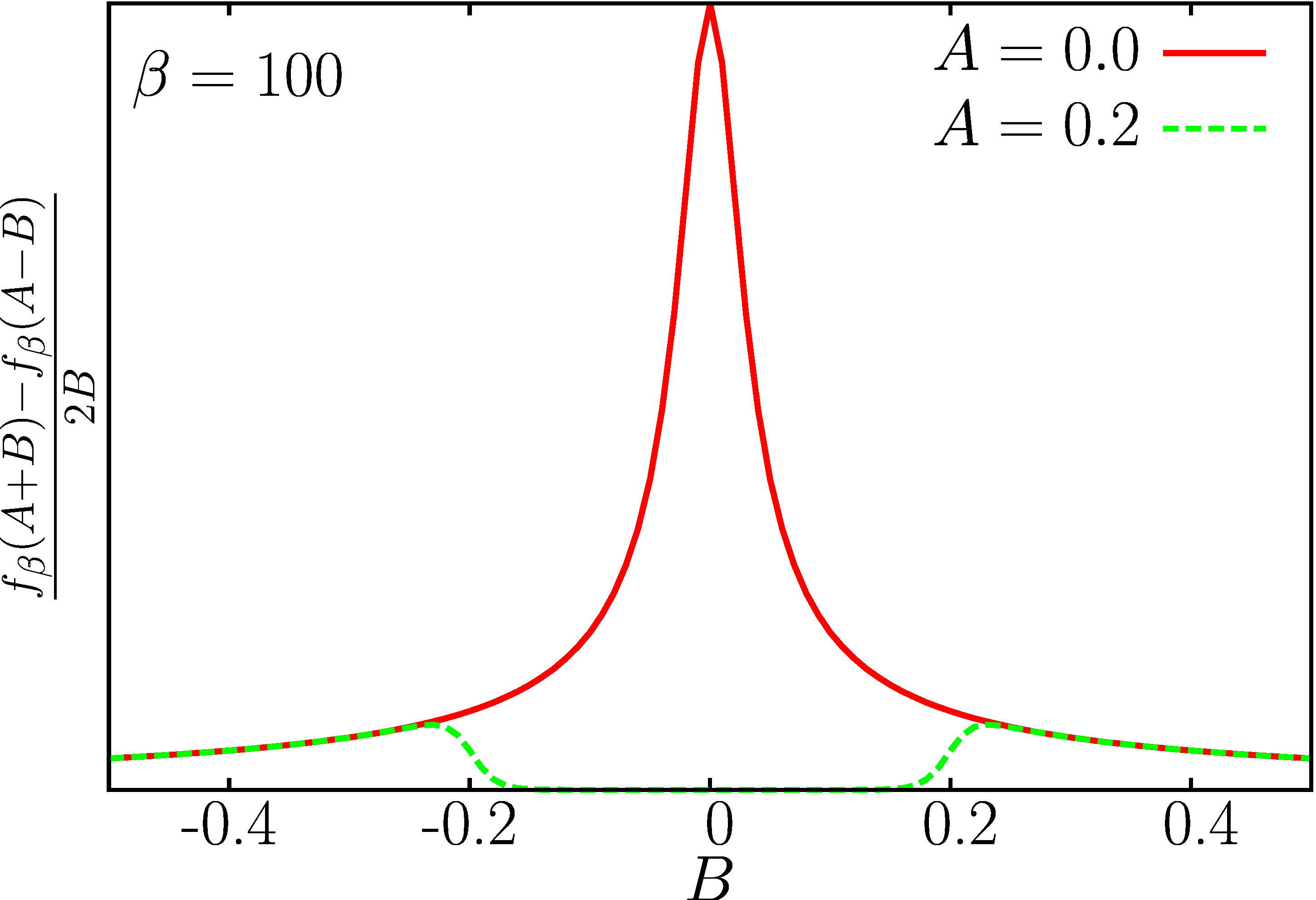
Figure 2: Sketch of the function $\beta a_{k}^{\sigma,-\sigma}(\varDelta_{{\rm s}}^{{\scriptscriptstyle{\rm s}}})$ multiplying ${\varDelta_{{\rm s}}^{{\scriptscriptstyle{\rm s}}}}_{k}$ into the coefficients for $\chi_{{\rm s}}(\boldsymbol{r},\boldsymbol{r}^{\prime})$. While being always non-zero, the coefficient function at $B=0$ behaves as $-(\beta/2)/\cosh\bigl{(}\beta(E_{k\sigma}^{+}+E_{k\sigma}^{-})/2\bigr{)}$ and thus becomes exponentially small with decreasing temperature.

. We thus observe that the order parameter $\chi_{{\rm s}}(\boldsymbol{r},\boldsymbol{r}^{\prime})$ is only weakly dependent on the potential matrix elements ${\varDelta_{{\rm s}}^{{\scriptscriptstyle{\rm s}}}}_{i}$ that correspond to states below the splitting energy $A$. Still, this does not invalidate the conclusion that at any finite temperature a continuously vanishing order parameter implies a continuously vanishing pair potential. We thus expect that (at low splitting) we can use the linearized Sham-Schlüter equation (157). In the following, we use a breve on top of linearized entities such as $\breve{S}_{\beta_{{\scriptscriptstyle{\rm c}}}}=\lim_{|\varDelta_{{\rm s}}^{{\scriptscriptstyle{\rm s}}}|\rightarrow 0}S_{\beta}[\varDelta_{{\rm s}}^{{\scriptscriptstyle{\rm s}}}]$ and Eq. (157) can be solved from the condition

$$\det\breve{S}_{\beta_{{\scriptscriptstyle{\rm c}}}}=0\,,$$ (166)

where $\beta_{{\scriptscriptstyle{\rm c}}}=1/T_{{\scriptscriptstyle{\rm c}}}$. The right eigenvector of $\breve{S}_{\beta_{{\scriptscriptstyle{\rm c}}}}$ is proportional to $\varDelta_{{\rm s}}^{{\scriptscriptstyle{\rm s}}}$. To compute the small $\varDelta_{{\rm s}}^{{\scriptscriptstyle{\rm s}}}$ limit of $\breve{S}_{\beta_{{\scriptscriptstyle{\rm c}}}}$ we first investigate the behavior of $|u_{k\sigma}^{k\alpha}|^{2}$, $|v_{k-\sigma}^{-k\alpha}|^{2}$ and $E_{k\sigma}^{\alpha}$ separately where we find

$$\lim_{|\varDelta_{{\rm s}}^{{\scriptscriptstyle{\rm s}}}|\rightarrow 0}|u_{k\sigma}^{k\alpha}|^{2} = \updelta_{\alpha,{\rm sign}(\varepsilon_{k\sigma}+\varepsilon_{-k-\sigma})}\,,$$ (167)

$$\lim_{|\varDelta_{{\rm s}}^{{\scriptscriptstyle{\rm s}}}|\rightarrow 0}|v_{k-\sigma}^{-k\alpha}|^{2} = \updelta_{\alpha,-{\rm sign}(\varepsilon_{k\sigma}+\varepsilon_{-k-\sigma})}\,,$$ (168)

$$\lim_{|\varDelta_{{\rm s}}^{{\scriptscriptstyle{\rm s}}}|\rightarrow 0}E_{k\sigma}^{\alpha} = \updelta_{\alpha,{\rm sign}(\varepsilon_{k\sigma}+\varepsilon_{-k-\sigma})}\varepsilon_{k\sigma}$$ (169)

$$- \updelta_{\alpha,-{\rm sign}(\varepsilon_{k\sigma}+\varepsilon_{-k-\sigma})}\varepsilon_{-k,-\sigma}\,.$$

Also we see that

$$\lim_{|\varDelta_{{\rm s}}^{{\scriptscriptstyle{\rm s}}}|\rightarrow 0}|u_{k\sigma}^{k\alpha}|^{2}|v_{k-\sigma}^{-k\alpha}|^{2}=\lim_{|\varDelta_{{\rm s}}^{{\scriptscriptstyle{\rm s}}}|\rightarrow 0}u_{k\sigma}^{k\alpha}{v_{k-\sigma}^{-k\alpha}}^{\ast}=0\,.$$ (170)

Thus it is straightforward to arrive at

$${\mbox{$\breve{S}_{\beta}^{{\scriptscriptstyle\text{M}}}$}}_{kk^{\prime}}=-2\delta_{kk^{\prime}}P_{{\rm s}}(\varepsilon_{k\uparrow},-\varepsilon_{-k\downarrow})$$ (171)

and

$${\mbox{$\breve{S}_{\beta}^{{\scriptscriptstyle\mathfrak{D}}}$}}_{kk^{\prime}}=$$

$$\frac{\delta_{kk^{\prime}}}{\varepsilon_{k\uparrow}\!+\!\varepsilon_{-k,\downarrow}}\sum_{ql}\Bigl{(}|g_{kl\uparrow}^{q}|^{2}\bigl{(}L(\varOmega_{q},\varepsilon_{k\uparrow},\varepsilon_{l\uparrow},\varepsilon_{k\uparrow})+$$

$$+L(\varOmega_{q},\varepsilon_{k\uparrow},-\varepsilon_{l\uparrow},\varepsilon_{k\uparrow})-L(\varOmega_{q},\varepsilon_{k\uparrow},\varepsilon_{l\uparrow},-\varepsilon_{-k,\downarrow})$$

$$-L(\varOmega_{q},\varepsilon_{k\uparrow},-\varepsilon_{l\uparrow},-\varepsilon_{-k,\downarrow})\bigr{)}+$$

$$+|g_{-k,-l\downarrow}^{q}|^{2}\bigl{(}L(\varOmega_{q},\varepsilon_{-k\downarrow},\varepsilon_{-l\downarrow},\varepsilon_{-k\downarrow})+$$

$$+L(\varOmega_{q},\varepsilon_{-k\downarrow},-\varepsilon_{-l\downarrow},\varepsilon_{-k\downarrow})-L(\varOmega_{q},\varepsilon_{-k\downarrow},\varepsilon_{-l\downarrow},-\varepsilon_{k\uparrow})$$

$$-L(\varOmega_{q},\varepsilon_{-k\downarrow},-\varepsilon_{-l\downarrow},-\varepsilon_{k\uparrow})\bigr{)}\,.$$ (172)

Moreover

$${\mbox{$\breve{S}_{{\scriptscriptstyle\text{ph}}\beta}^{{\scriptscriptstyle\mathfrak{C}}}$}}_{kk^{\prime}}=$$

$$-2\!\sum_{q}\!\frac{g_{kk^{\prime}\uparrow}^{q}g_{-k,-k^{\prime},\downarrow}^{-q}}{|\varepsilon_{k^{\prime}\uparrow}+\varepsilon_{-k^{\prime},\downarrow}|}\bigl{(}L(\varOmega_{q},\varepsilon_{k\uparrow},\breve{E}_{k^{\prime}\uparrow}^{+},-\varepsilon_{-k\downarrow})+$$

$$+L(\varOmega_{q},\varepsilon_{-k\downarrow},\breve{E}_{-k^{\prime}\downarrow}^{+},-\varepsilon_{k\uparrow})\bigr{)}$$ (173)

and

$${\mbox{$\breve{S}_{{\scriptscriptstyle\text{C}}\beta}^{{\scriptscriptstyle\mathfrak{C}}}$}}_{kk^{\prime}}=-2{W_{kk^{\prime},-k,-k^{\prime}}^{{\scriptscriptstyle\text{stat}}}}_{\uparrow,\downarrow}\times$$

$$\times P_{{\rm s}}(\breve{E}_{k^{\prime}\uparrow}^{+},-\breve{E}_{-k^{\prime}\downarrow}^{+})P_{{\rm s}}(\varepsilon_{k\uparrow},-\!\varepsilon_{-k\downarrow})\,.$$ (174)

III.3.2 Non-linear Gap-Equation

Far from $T_{{\scriptscriptstyle{\rm c}}}$ or in those parts of the phase diagram where the SC transition is of first order we need to use the non-linear Sham-Schlüter equation, because a solution with small $|{\varDelta_{{\rm s}}^{{\scriptscriptstyle{\rm s}}}}_{k}|$ may not exist. The most common method to solve an equation of type Eq. (157) is to use an invertible splitting matrix $\mathcal{S}$ and cast $S_{\beta}[\varDelta_{{\rm s}}^{{\scriptscriptstyle{\rm s}}}]\cdot\varDelta_{{\rm s}}^{{\scriptscriptstyle{\rm s}}}=0$ into a fixed point problem

$$\varDelta_{{\rm s}}^{{\scriptscriptstyle{\rm s}}}=\mathcal{K}_{\mathcal{\mathcal{S}}}[\varDelta_{{\rm s}}^{{\scriptscriptstyle{\rm s}}}]\cdot\varDelta_{{\rm s}}^{{\scriptscriptstyle{\rm s}}}\quad\mathcal{K}_{\mathcal{S}}=\mathcal{S}^{-1}\cdot(S_{\beta}+\mathcal{S})\,.$$ (175)

This is the gap equation of SpinSCDFT. In the spin degenerate limit the choice $\mathcal{S}=-\breve{S}_{\beta}^{{\scriptscriptstyle\text{M}}}$ leads to the SCDFT gap equation given in Ref. Lüders et al., 2005. We point out that while we can show that all ${\mbox{$\breve{S}_{\beta}^{{\scriptscriptstyle\text{M}}}$}}_{k,k}<0$ at $\varepsilon_{k\sigma}+\varepsilon_{-k,-\sigma}=0$ ${\mbox{$\breve{S}_{\beta}^{{\scriptscriptstyle\text{M}}}$}}_{k,k}\sim\exp\bigl{(}-\frac{1}{2}\beta(\varepsilon_{k\sigma}-\varepsilon_{-k,-\sigma})\bigr{)}$ and is thus a numerically problematic object. In the implementation that we describe in detail in II we find that a good choice is $\mathcal{S}=-S_{\beta}^{{\scriptscriptstyle\text{M}}}(\varepsilon_{k\sigma}=\varepsilon_{-k,-\sigma})$. Obviously in the spin degenerate limit we recover the formulas given in Ref. Lüders et al., 2005. In part II we will also discuss the properties of the splitting versus temperature diagram for a simple system in detail.

IV Eliashberg equations

In the KS-SpinSCDFT formalism, interaction effects are mimicked by the $xc$-potential that is an (implicit) functional of the densities. While the functional construction and the additional complications of the SC KS system pose additional algebraic complexity, the result is a numerically cheaper computational scheme. This is owed to the fact that Matzubara summations in the self-energy are not computed numerically but absorbed into the analytic structure of the $xc$-potential. Likely, the knowledge of the interacting self-energy is essential to a future improvement of the presented functional. The self-energy Eq. (100) in turn is constructed via diagrammatic perturbation theory using the electronic and phononic GF similar to Sec. III.3, and involving the solution of a Dyson equation. In the present section, we develop this direct many-body scheme to obtain the electronic GF. The final set of equations generalize the ones of Eliashberg Eliashberg (1960) and we refer to them with the same name. Ref. Vonsovsky et al., 1982 discusses similar equations in a different notation with a limitation to isotropic system with a homogenous splitting parameter.

IV.1 Solving the Dyson Equation

The starting point of the derivation of the Eliashberg equations is the Dyson equation of a SC Eq. (99). We represent it in the basis of normal state, zero temperature KS orbitals $\{\vec{\varphi}_{i\sigma}(\boldsymbol{r})\}$ defined in Eq. (44). We use the Nambu-Anderson Nambu (1960); Anderson (1958) notation similar to that used in the functional derivation and in Eq. 118. The Dyson equation reads

$$\bar{G}_{ij}(\omega_{n})=\bar{G}_{ij}^{{\scriptscriptstyle{\rm KS}}}(\omega_{n})+\!\sum_{kl}\!\!\bar{G}_{ik}^{{\scriptscriptstyle{\rm KS}}}(\omega_{n})\cdot\bar{\varSigma}_{kl}^{{\scriptscriptstyle{\rm s}}}(\omega_{n})\cdot\bar{G}_{lj}(\omega_{n}),$$ (176)

where $\bar{G}_{ij}^{{\scriptscriptstyle{\rm KS}}}$ is the SC KS GF and $\bar{\varSigma}_{ij}^{{\scriptscriptstyle{\rm s}}}(\omega_{n})=\bar{\varSigma}_{{\scriptscriptstyle{\rm xc}}ij}(\omega_{n})-\bar{v}_{{\scriptscriptstyle{\rm xc}}ij}$ where $\bar{\varSigma}_{{\scriptscriptstyle{\rm xc}}ij}(\omega_{n})$ is the Nambu exchange and correlation self-energy that also includes the phononic Hartree diagram Linscheid and Essenberger . $\bar{v}_{{\scriptscriptstyle{\rm xc}}ij}$ are the matrix elements of the $xc$-potential of the SC KS system. Note that the SC KS GF is not diagonal in the space of $\{\vec{\varphi}_{i\sigma}(\boldsymbol{r})\}$. Similar to our approach in SpinSCDFT of Section III we assume that $\{\vec{\varphi}_{i\sigma}(\boldsymbol{r})\}$ is a good approximation to the quasi particle state, i.e. $\bar{\varSigma}_{kl}^{{\scriptscriptstyle{\rm s}}}(\omega_{n})$ and $\bar{G}_{ij}(\omega_{n})$ are essentially diagonal. We use similar diagrams (Eq. (109) and (110)) as for the functional construction of SpinSCDFT in Subsection III.3 namely the phononic and Coulomb exchange diagram. Again similarly (compare Sub. III.3) we drop the Coulomb corrections on the Nambu diagonal that add to the $xc$ potential. Further we assume, as in the SDA of Sec. III.1.2, that the pairing occurs only between time reversed states Anderson (1959). This means we only consider singlet SC. Starting from Eq. (176) in the form $\bar{G}_{ij}(\omega_{n})=\bigl{(}{\mbox{$\bar{G}_{ij}^{{\scriptscriptstyle{\rm KS}}}$}}^{-1}(\omega_{n})-\bar{\varSigma}_{ij}^{{\scriptscriptstyle{\rm s}}}(\omega_{n})\bigr{)}^{-1}$, under the mentioned approximations, the Dyson equation is a $4\times 4$ matrix equation that can be solved analytically. Note that here we do not substitute the SC KS GF for the interaction GF in the self-energy (as was done in the functional construction of SpinSCDFT of Sec. III.3). This is the main difference in the two approaches so far.

IV.1.1 Analytic Inversion of the Dyson Equation

The easiest way to invert the right hand side of the Dyson equation

$$\bar{G}_{ij}(\omega_{n})=\bigl{(}{\mbox{$\bar{G}_{ij}^{{\scriptscriptstyle{\rm KS}}}$}}^{-1}(\omega_{n})-\bar{\varSigma}_{ij}^{{\scriptscriptstyle{\rm s}}}(\omega_{n})\bigr{)}^{-1}\,,$$ (177)

is to identify contributions of the self-energy that add to a given variable of the inverse SC KS GF ${\mbox{$\bar{G}_{ij}^{{\scriptscriptstyle{\rm KS}}}$}}^{-1}(\omega_{n})$ of Eq. (138). We summarize these self-energy contributions in Table 1

SE part	${\mbox{$\bar{G}^{{\scriptscriptstyle{\rm KS}}}$}}^{-1}$ part	Basis vector	Eliashberg
$\varSigma_{k}^{\omega}(\omega_{n})$	${\rm i}\omega_{n}$	$\tau_{0}\sigma_{0}$	$Z_{k}(\omega_{n})$
$A_{k}^{\omega}(\omega_{n})$	$-$	$\tau_{0}\sigma_{z}$	$\tilde{A}_{k}^{\omega}(\omega_{n})$
$\varSigma_{k}^{\varepsilon}(\omega_{n})$	$(\varepsilon_{k\uparrow}+\varepsilon_{-k\downarrow})/2$	$\tau_{z}\sigma_{0}$	$\tilde{\varepsilon}_{k}(\omega_{n})$
$\varSigma_{k}^{J}(\omega_{n})$	$(\varepsilon_{k\uparrow}-\varepsilon_{-k\downarrow})/2$	$\tau_{z}\sigma_{z}$	$\tilde{J}_{k}(\omega_{n})$
$\varSigma_{k}^{{\scriptscriptstyle\Re\Delta}}(\omega_{n})$	$\Re{\varDelta_{{\rm s}}^{{\scriptscriptstyle{\rm s}}}}_{k}$	$(\mbox{i}\tau_{y})(\mbox{i}\sigma_{y})$	$\varDelta_{k}^{{\scriptscriptstyle\text{E}}}(\omega_{n})$
$\mbox{i}\varSigma_{k}^{{\scriptscriptstyle\Im\Delta}}(\omega_{n})$	$\mbox{i}\Im{\varDelta_{{\rm s}}^{{\scriptscriptstyle{\rm s}}}}_{k}$	$\tau_{x}(\mbox{i}\sigma_{y})$	$\varDelta_{k}^{{\scriptscriptstyle\text{E}}\star}(\omega_{n})$

Table 1: Self-energy contributions, the variable of the inverse SC KS GF which they add to and the basis vector. E.g. along the $\tau_{0}\sigma_{0}$ direction in Spin and Nambu space ${\rm i}\omega_{n}+\varSigma_{k}^{\omega}(\omega_{n})$. In the last column we give the related Eliashberg property. Note that $\varDelta_{k}^{{\scriptscriptstyle\text{E}}}\sim\varSigma_{k}^{{\scriptscriptstyle\Re\Delta}}+\mbox{i}\varSigma_{k}^{{\scriptscriptstyle\Im\Delta}}$ and $\varDelta_{k}^{{\scriptscriptstyle\text{E}}\star}(\omega_{n})\sim\varSigma_{k}^{{\scriptscriptstyle\Re\Delta}}-\mbox{i}\varSigma_{k}^{{\scriptscriptstyle\Im\Delta}}$.

. This means we decompose the Nambu and spin matrix $\bar{\varSigma}_{kl}^{{\scriptscriptstyle{\rm s}}}(\omega_{n})$ along the vectors $\tau_{0}\sigma_{0}$, $\tau_{z}\sigma_{0}$ and so on. Then, we name the self-energy contributions according to the property of the SC KS GF they add to in Eq. (177) and indicate the property in the superscript. For example the Matsubara frequency variable of the inverse SC KS GF points along the $\tau_{0}\sigma_{0}$ axis in spin and Nambu space. Correspondingly the self-energy part along basis vector is referred to as $\varSigma_{k}^{\omega}(\omega_{n})$. In the following we use $|g_{kk^{\prime}\sigma}^{q}|^{2}=|g_{k^{\prime}k\sigma}^{-q}|^{2}$, $D_{q,-q}^{{\scriptscriptstyle{\rm 0}}}=D_{-q,q}^{{\scriptscriptstyle{\rm 0}}}$ and ${W_{kk^{\prime}k^{\prime}k}^{{\scriptscriptstyle\text{stat}}}}_{\sigma\sigma}={W_{k^{\prime}kkk^{\prime}}^{{\scriptscriptstyle\text{stat}}}}_{\sigma\sigma}$, Then the equations for the corresponding scalar self-energy components read

$$\varSigma_{k}^{\omega}(\omega_{n}) = \frac{1}{4}\sum_{\sigma\alpha k^{\prime}q}\frac{1}{\beta}\sum_{n^{\prime}}(\tau_{0})_{\alpha\alpha}D_{q,-q}^{{\scriptscriptstyle{\rm 0}}}(\omega_{n^{\prime}}-\omega_{n})\times$$ (178)

$$\times|g_{kk^{\prime}\sigma}^{q}|^{2}\bar{G}_{k^{\prime}\sigma,k^{\prime}\sigma}^{{\scriptscriptstyle\alpha,\alpha}}(\omega_{n^{\prime}})$$

$$A_{k}^{\omega}(\omega_{n}) = \frac{1}{4}\sum_{\sigma\alpha k^{\prime}q}\frac{1}{\beta}\sum_{n^{\prime}}\frac{(\tau_{0})_{\alpha\alpha}}{{\rm sign}(\sigma)}D_{q,-q}^{{\scriptscriptstyle{\rm 0}}}(\omega_{n^{\prime}}-\omega_{n})\times$$ (179)

$$\times|g_{kk^{\prime}\sigma}^{q}|^{2}\bar{G}_{k^{\prime}\sigma,k^{\prime}\sigma}^{{\scriptscriptstyle\alpha,\alpha}}(\omega_{n^{\prime}})$$

$$\varSigma_{k}^{\varepsilon}(\omega_{n}) = \frac{1}{4}\sum_{\sigma\alpha k^{\prime}q}\frac{1}{\beta}\sum_{n^{\prime}}(\tau_{z})_{\alpha\alpha}D_{q,-q}^{{\scriptscriptstyle{\rm 0}}}(\omega_{n^{\prime}}-\omega_{n})\times$$ (180)

$$\times|g_{kk^{\prime}\sigma}^{q}|^{2}\bar{G}_{k^{\prime}\sigma,k^{\prime}\sigma}^{{\scriptscriptstyle\alpha,\alpha}}(\omega_{n^{\prime}})$$

$$\varSigma_{k}^{J}(\omega_{n}) = \frac{1}{4}\sum_{\sigma\alpha k^{\prime}q}\frac{1}{\beta}\sum_{n^{\prime}}\frac{(\tau_{z})_{\alpha\alpha}}{{\rm sign}(\sigma)}D_{q,-q}^{{\scriptscriptstyle{\rm 0}}}(\omega_{n^{\prime}}-\omega_{n})\times$$ (181)

$$\times|g_{kk^{\prime}\sigma}^{q}|^{2}\bar{G}_{k^{\prime}\sigma,k^{\prime}\sigma}^{{\scriptscriptstyle\alpha,\alpha}}(\omega_{n^{\prime}})\,.$$

Note that $A_{k}^{\omega}(\omega_{n})$ stands out in the sense that the SC KS GF has no contribution along this direction in Nambu and spin space. On the Nambu-off-diagonal we similarly introduce

$$\varSigma_{k}^{{\scriptscriptstyle\Im\Delta}}(\omega_{n}) = \!-\!\sum_{\sigma k^{\prime}}\frac{1}{\beta}\sum_{n^{\prime}}\frac{\text{sign}(\sigma)}{4\mbox{i}}\bigl{(}\sum_{q}D_{q,-q}^{{\scriptscriptstyle{\rm 0}}}(\omega_{n^{\prime}}-\omega_{n})\times$$ (182)

$$\times g_{kk^{\prime}\sigma}^{q}g_{-k,-k^{\prime},-\sigma}^{-q}+{W_{kk^{\prime},-k,-k^{\prime}}^{{\scriptscriptstyle\text{stat}}}}_{\sigma,-\sigma}\bigr{)}\times$$

$$\times\sum_{\alpha}(\tau_{x})_{\alpha\alpha}\bar{G}_{k^{\prime}\sigma,-k^{\prime},-\sigma}^{{\scriptscriptstyle\alpha,-\alpha}}(\omega_{n^{\prime}})$$

$$\varSigma_{k}^{{\scriptscriptstyle\Re\Delta}}(\omega_{n}) = \!-\!\sum_{\sigma k^{\prime}}\frac{1}{\beta}\sum_{n^{\prime}}\frac{\text{sign}(\sigma)}{4}\bigl{(}\sum_{q}D_{q,-q}^{{\scriptscriptstyle{\rm 0}}}(\omega_{n^{\prime}}-\omega_{n})\times$$ (183)

$$g_{k^{\prime}k\sigma}^{q}g_{-k^{\prime},-k,-\sigma}^{-q}+{W_{k^{\prime}k,-k^{\prime},-k}^{{\scriptscriptstyle\text{stat}}}}_{\sigma,-\sigma}\bigr{)}\times$$

$$\times\sum_{\alpha}({\rm i}\tau_{y})_{\alpha\alpha}\bar{G}_{k^{\prime}\sigma,-k^{\prime},-\sigma}^{{\scriptscriptstyle\alpha,-\alpha}}(\omega_{n^{\prime}})\,.$$

Here we introduce $B_{k}(\omega_{n})=\varSigma_{k}^{{\scriptscriptstyle\Re\Delta}}(\omega_{n})+{\rm i}\varSigma_{k}^{{\scriptscriptstyle\Im\Delta}}(\omega_{n})$ and $B_{k}^{\star}(\omega_{n})=\varSigma_{k}^{{\scriptscriptstyle\Re\Delta}}(\omega_{n})-{\rm i}\varSigma_{k}^{{\scriptscriptstyle\Im\Delta}}(\omega_{n})$

$$B_{k}(\omega_{n}) = -\sum_{\sigma k^{\prime}}\frac{1}{\beta}\sum_{n^{\prime}}\frac{\text{sign}(\sigma)}{2}\bigl{(}\sum_{q}D_{q,-q}^{{\scriptscriptstyle{\rm 0}}}(\omega_{n^{\prime}}-\omega_{n})\times$$ (184)

$$\times g_{kk^{\prime}\sigma}^{q}g_{-k,-k^{\prime},-\sigma}^{-q}+{W_{kk^{\prime},-k,-k^{\prime}}^{{\scriptscriptstyle\text{stat}}}}_{\sigma,-\sigma}\bigr{)}\times$$

$$\times\bar{G}_{k^{\prime}\sigma,-k^{\prime},-\sigma}^{{\scriptscriptstyle 1,-1}}(\omega_{n^{\prime}})$$

$$B_{k}^{\star}(\omega_{n}) = \sum_{\sigma k^{\prime}}\frac{1}{\beta}\sum_{n^{\prime}}\frac{\text{sign}(\sigma)}{2}\bigl{(}\sum_{q}D_{q,-q}^{{\scriptscriptstyle{\rm 0}}}(\omega_{n^{\prime}}-\omega_{n})\times$$ (185)

$$\times g_{k^{\prime}k\sigma}^{q}g_{-k^{\prime},-k,-\sigma}^{-q}+{W_{k^{\prime}k,-k^{\prime},-k}^{{\scriptscriptstyle\text{stat}}}}_{\sigma,-\sigma}\bigr{)}\times$$

$$\times\bar{G}_{k^{\prime}\sigma,-k^{\prime},-\sigma}^{{\scriptscriptstyle-1,1}}(\omega_{n^{\prime}})\,.$$

If both $\Sigma_{k}^{{\scriptscriptstyle\Re\Delta}}$ and $\Sigma_{k}^{{\scriptscriptstyle\Im\Delta}}$ are real $B_{k}^{\star}$ is the complex conjugate of $B_{k}$. Further, for the same reasons discussed in Sec. III.1.2, we do not consider the possibility that triplet self-energy contributions appear. It is important to remark that, just as in the usual derivation of the spin degenerate Eliashberg equations, the $k$ dependence of all self-energy parts is generated via the $k$ dependence of the Couplings $|g_{kk^{\prime}\sigma}^{q}|^{2}$ and in addition ${W_{k^{\prime}k,-k^{\prime},-k}^{{\scriptscriptstyle\text{stat}}}}_{\sigma,-\sigma}$ on the Nambu off diagonal.

Introducing the mass renormalization function $Z_{k}(\omega_{n})$ as

$$Z_{k}(\omega_{n})=1+\text{i}\varSigma_{k}^{\omega}(\omega_{n})\!/\omega_{n}\,,$$ (186)

we can rewrite some of the above equations by including $Z_{k}^{{\scriptscriptstyle\text{E}}}(\omega_{n})$ into the self-energy parts:

$$\varDelta_{k}^{{\scriptscriptstyle\text{E}}}(\omega_{n}) = B_{k}(\omega_{n})\!/Z_{k}(\omega_{n})$$ (187)

$$\varDelta_{k}^{{\scriptscriptstyle\text{E}}\star}(\omega_{n}) = B_{k}^{\star}(\omega_{n})\!/Z_{k}(\omega_{n})$$ (188)

$$\tilde{\varepsilon}_{k}(\omega_{n}) = \bigl{(}(\varepsilon_{k\uparrow}+\varepsilon_{-k\downarrow})\!/2+\varSigma_{k}^{\varepsilon}(\omega_{n})\bigr{)}\!/Z_{k}(\omega_{n})$$ (189)

$$\tilde{J}_{k}(\omega_{n}) = \bigl{(}(\varepsilon_{k\uparrow}-\varepsilon_{-k\downarrow})\!/2+\varSigma_{k}^{J}(\omega_{n})\bigr{)}\!/Z_{k}(\omega_{n})$$ (190)

$$\tilde{A}_{k}^{\omega}(\omega_{n}) = A_{k}^{\omega}(\omega_{n})\!/Z_{k}(\omega_{n})\,.$$ (191)

Then by introducing the abbreviation

$$\mathfrak{F}_{k\sigma}(\omega_{n}) = \Bigl{(}\bigl{(}\tilde{\varepsilon}_{k}(\omega_{n})+\mbox{sign}(\sigma)\tilde{A}_{k}^{\omega}(\omega_{n})\bigr{)}^{2}$$ (192)

$$+\varDelta_{k}^{{\scriptscriptstyle\text{E}}}(\omega_{n})\varDelta_{k}^{{\scriptscriptstyle\text{E}}\star}(\omega_{n})\Bigr{)}^{\frac{1}{2}}\,,$$

and suppressing the arguments $\omega_{n}$, we arrive at the formulas for non-vanishing SC GF components

$$\bar{G}_{k\sigma,k\sigma}^{{\scriptscriptstyle 1,1}} = \!\frac{1}{2\mathfrak{F}_{k\sigma}Z_{k}}\!\sum_{\alpha}\!\frac{\mathfrak{F}_{k\sigma}+\alpha\bigl{(}\tilde{\varepsilon}_{k}+\mbox{sign}(\sigma)\tilde{A}_{k}^{\omega}\bigr{)}}{\text{i}\omega_{n}-\mbox{sign}(\sigma)\tilde{J}_{k}-\alpha\mathfrak{F}_{k\sigma}}$$

$$\bar{G}_{k\sigma,k\sigma}^{{\scriptscriptstyle-1,-1}} = \!\frac{1}{2\mathfrak{F}_{k,-\sigma}Z_{k}}\!\sum_{\alpha}\!\frac{\mathfrak{F}_{k,-\sigma}\!+\alpha\bigl{(}\tilde{\varepsilon}_{k}\!-\!\mbox{sign}(\sigma)\!\tilde{A}_{k}^{\omega}\bigr{)}}{\text{i}\omega_{n}+\mbox{sign}(\sigma)\tilde{J}_{k}+\alpha\mathfrak{F}_{k,-\sigma}}$$

$$\bar{G}_{k\sigma,-k,-\sigma}^{{\scriptscriptstyle 1,-1}} = \!\frac{1}{2\mathfrak{F}_{k\sigma}Z_{k}}\!\sum_{\alpha}\!\frac{\mbox{sign}(\sigma)\alpha\varDelta_{k}^{{\scriptscriptstyle\text{E}}}}{\text{i}\omega_{n}-\mbox{sign}(\sigma)\tilde{J}_{k}-\alpha\mathfrak{F}_{k\sigma}}$$

$$\bar{G}_{k\sigma,-k,-\sigma}^{{\scriptscriptstyle-1,1}} = \!\frac{1}{2\mathfrak{F}_{k,-\sigma}Z_{k}}\!\sum_{\alpha}\!\frac{\mbox{sign}(\sigma)\alpha\varDelta_{k}^{{\scriptscriptstyle\text{E}}\star}}{\text{i}\omega_{n}+\mbox{sign}(\sigma)\tilde{J}_{k}+\alpha\mathfrak{F}_{k,-\sigma}}\,.$$

We have thus expressed the GF in terms of the self-energy components (Eq. (187) to (191)) explicitly. The coupled set of equations Eq. (187) to (191) are the Eliashberg equations and have to be solved according to the scheme:

1. Start with the coupling matrix elements $g_{k^{\prime}k\sigma}^{q}$ and ${W_{k^{\prime}k,-k^{\prime},-k}^{{\scriptscriptstyle\text{stat}}}}_{\sigma,-\sigma}$ and an initial guess for the self-energy components $\varDelta_{k}^{{\scriptscriptstyle\text{E}}},\varDelta_{k}^{{\scriptscriptstyle\text{E}}\star},\tilde{\varepsilon}_{k},\tilde{J}_{k}$ and $\tilde{A}_{k}^{\omega}$.

2. Evaluate Eq. (187) to (191). They are closed in the sense that inserting the equations of this section $\varDelta_{k}^{{\scriptscriptstyle\text{E}}},\varDelta_{k}^{{\scriptscriptstyle\text{E}}\star},\tilde{\varepsilon}_{k},\tilde{J}_{k}$ and $\tilde{A}_{k}^{\omega}$ only dependent on each other and the coupling matrix elements $g_{k^{\prime}k\sigma}^{q}$ and ${W_{k^{\prime}k,-k^{\prime},-k}^{{\scriptscriptstyle\text{stat}}}}_{\sigma,-\sigma}$.

3. Construct a new self-energy and iterate from point 2, up to self-consistency.

$\tilde{A}_{k}^{\omega}$ is a peculiar object because it generates a spin imbalance in the particle as compared to the hole channel. To understand the effect of $\tilde{A}_{k}^{\omega}$ consider the following self-consistent cycle. We start the iteration of these equations with $\tilde{A}_{k}^{\omega}=0$ and $\varSigma_{k}^{{\scriptscriptstyle\Im\Delta}}=0$. Then follows $\bar{G}_{k\sigma,-k,-\sigma}^{{\scriptscriptstyle 1,-1}}=\bar{G}_{k,-\sigma,-k\sigma}^{{\scriptscriptstyle-1,1}}$ which results in $B_{k}^{\star}=B_{k}$ and no self-energy part $\varSigma_{k}^{{\scriptscriptstyle\Im\Delta}}$ is generated. Further, because $\bar{G}_{k\sigma,k\sigma}^{{\scriptscriptstyle-1,-1}}=\bar{G}_{k,-\sigma k,-\sigma}^{{\scriptscriptstyle 1,1}}$ we find then that $\tilde{A}_{k}^{\omega}$ is proportional to the difference of the interaction in the spin channels $\tilde{A}_{k}^{\omega}\propto|g_{kk^{\prime}\uparrow}^{q}|^{2}-|g_{kk^{\prime}\downarrow}^{q}|^{2}$. If now the interaction is independent on the spin channel $|g_{kk^{\prime}\uparrow}^{q}|^{2}-|g_{kk^{\prime}\downarrow}^{q}|^{2}=0$ then $\tilde{A}_{k}^{\omega}$ also remains zero and we are at our starting point. Thus we conclude that for spin independent couplings $\varSigma_{k}^{{\scriptscriptstyle\Im\Delta}}$ and $\tilde{A}_{k}^{\omega}$ remain zero during iteration. If the interaction is spin dependent $|g_{kk^{\prime}\uparrow}^{q}|^{2}-|g_{kk^{\prime}\downarrow}^{q}|^{2}\neq 0$ the self-consistency iteration will generate a spin imbalance in the GF. This is not surprising because the up and down single particle spectrum is altered in a different way by the interaction. Then a non-vanishing $\varSigma_{k}^{{\scriptscriptstyle\Im\Delta}}$ cannot be excluded.

For future reference we extract the renormalized energy dependence $\tilde{\varepsilon}_{k}$ of the GF as it appears in the self-energy Eq. (178) to (181) and Eq. (184) and (185). With the abbreviation

$$a_{k}(\omega_{n}) = (\tilde{A}_{k}^{\omega z})^{2}+\varDelta_{k}^{{\scriptscriptstyle\text{E}}}\varDelta_{k}^{{\scriptscriptstyle\text{E}}\star}+\omega_{n}^{2}-(\tilde{J}_{k})^{2}$$ (197)

we obtain ($b=0,z$)

$$\sum_{\alpha}(\tau_{b})_{\alpha\alpha}\bar{G}_{k\sigma,k\sigma}^{{\scriptscriptstyle\alpha,\alpha}}=$$

$$\!=\!\sum_{\alpha}\!\!\frac{(\tau_{b})_{\alpha\alpha}}{Z_{k}}\frac{\alpha\Bigl{(}\tilde{\varepsilon}_{k}\!-\!\mbox{sign}(\sigma)\bigl{(}\tilde{J}_{k}\!+\!\alpha\tilde{A}_{k}^{\omega}\bigr{)}\Bigr{)}\!-\!\text{i}\omega_{n}}{a_{k}\!-\!\frac{2\alpha}{\mbox{sign}(\sigma)}\bigl{(}\text{i}\omega_{n}\tilde{J}_{k}\!+\!\tilde{A}_{k}^{\omega}\tilde{\varepsilon}_{k}\bigr{)}\!+\!\tilde{\varepsilon}_{k}^{2}}$$ (198)

and

$$\sum_{\sigma}\bar{G}_{k\sigma,-k,-\sigma}^{{\scriptscriptstyle 1,-1}}(\omega_{n})=$$

$$\!=\!-\frac{1}{Z_{k}}\sum_{\alpha}\frac{\varDelta_{k}^{{\scriptscriptstyle\text{E}}}}{a_{k}-\alpha\bigl{(}\text{i}\omega_{n}\tilde{J}_{k}+\tilde{A}_{k}^{\omega}\tilde{\varepsilon}_{k}\bigr{)}+\tilde{\varepsilon}_{k}^{2}}$$ (199)

IV.2 Analytic Integration of the Energy

In a numerical solution, the equations (187) to (191) have to be iterated until self-consistency is reached. Each self-consistent step requires to perform Matsubara summations in addition to the $k$ space summations which will be numerically demanding.

Note however that the $k$ space summations can be avoided using an approximation that is very common in the context of Eliashberg theory which is essentially to replace the couplings with their value at $\tilde{\varepsilon}_{k}(\omega_{n})=0$. The reason why this is sensible can be understood from the GF. From the above equation (198) one can easily see that $\bar{G}_{k\sigma,k\sigma}^{{\scriptscriptstyle 1,1}}(\omega_{n})-\bar{G}_{k\sigma,k\sigma}^{{\scriptscriptstyle-1,-1}}(\omega_{n})$ behaves as $\bigl{(}\tilde{\varepsilon}_{k}(\omega_{n})\bigr{)}^{-1}$ for large $\tilde{\varepsilon}_{k}(\omega_{n})$. In turn, $\bar{G}_{k\sigma k\sigma}^{{\scriptscriptstyle 1,1}}(\omega_{n})+\bar{G}_{k\sigma k\sigma}^{{\scriptscriptstyle-1,-1}}(\omega_{n})$ and the Nambu off-diagonal parts $\bar{G}_{k\sigma,-k,-\sigma}^{{\scriptscriptstyle\alpha,-\alpha}}(\omega_{n})$ behave as $\bigl{(}\tilde{\varepsilon}_{k}(\omega_{n})\bigr{)}^{-2}$ for large $\tilde{\varepsilon}_{k}(\omega_{n})$. Using this insight we see from the Eqs. (178), (179), (184) and (185) that $Z_{k}(\omega_{n}),\tilde{A}_{k}^{\omega}(\omega_{n}),\varDelta_{k}^{{\scriptscriptstyle\text{E}}}(\omega_{n})$ and $\varDelta_{k}^{{\scriptscriptstyle\text{E}}\star}(\omega_{n})$ are almost independent on the space $k$ belonging to large $\tilde{\varepsilon}_{k}$ because its contributions are suppressed by a factor $\bigl{(}\tilde{\varepsilon}_{k}(\omega_{n})\bigr{)}^{-2}$. Thus these quantities can be computed replacing the couplings with their value at $\tilde{\varepsilon}_{k}(\omega_{n})=0$.

With the integrand behaving as $\bigl{(}\tilde{\varepsilon}_{k}(\omega_{n})\bigr{)}^{-1}$ , the convergence of the Brillouin zone integrals in $\varSigma_{k}^{\varepsilon}(\omega_{n})$ and $\varSigma_{k}^{J}(\omega_{n})$ depend on the $k$-dependence of the couplings in an essential way, even on $k$ that correspond to a large $\tilde{\varepsilon}_{k}$. In particular, in absence of any $k$ dependence of the couplings $\varSigma_{k}^{\varepsilon}(\omega_{n})$ and $\varSigma_{k}^{J}(\omega_{n})$ diverge logarithmically. From the physical point of view $\varSigma_{k}^{\varepsilon}(\omega_{n})$ shifts the position of the Fermi energy and $\varSigma_{k}^{J}(\omega_{n})$ the magnetic splitting of quasiparticle states due to many-body interactions. These terms are zero if the system shows particle-hole symmetry and small in general (see also the discussion in Sec. III.3). Therefore we will discard these contributions completely and replace the couplings with their value at $\tilde{\varepsilon}_{k}(\omega_{n})=0$ entirely, reducing the computational costs significantly.

Another very effective simplification of the formalism comes from assuming the system to be isotropic in $k$. This means that the couplings will depend on $k$ only via the quasi particle energy $\varepsilon_{k\sigma}$. Here, we introduce the averaging operation on a generic function $F_{k\sigma}$ on equal center of energy and equal splitting surfaces according to

$$F_{\sigma}(\varepsilon,J) = \hat{I}_{k\sigma}(\varepsilon,J)F_{k\sigma}$$ (201)

$$= \frac{1}{\varrho(\varepsilon,J)}\sum_{k}\updelta(\frac{\varepsilon_{{\scriptscriptstyle{\rm sign}(\sigma)}k\uparrow}+\varepsilon_{-{\scriptscriptstyle{\rm sign}(\sigma)}k\downarrow}}{2}-\varepsilon)\times$$

$$\times\updelta(\frac{\varepsilon_{{\scriptscriptstyle{\rm sign}(\sigma)}k\uparrow}-\varepsilon_{-{\scriptscriptstyle{\rm sign}(\sigma)}k\downarrow}}{2}-J)F_{k\sigma}\,,$$

where the number of states on center of energy and splitting surfaces is given by $\varrho(\varepsilon,J)=\hat{I}_{k\sigma}(\varepsilon,J)\,1$. The subscript indices “$k\sigma"$ on $\hat{I}_{k\sigma}(\varepsilon,J)$ indicate the variables that are averaged. Note that we invert the sign of $\boldsymbol{k}$ for the $\sigma=\downarrow$ part which makes $\hat{I}_{k\sigma}(\varepsilon,J)F_{k\sigma}=\hat{I}_{-k,-\sigma}(\varepsilon,J)F_{-k,-\sigma}$. Now we define the analog of the Eliashberg function $\alpha^{\!2}\!F(\omega)$ Carbotte (1990); Allen and Mitrović (1983). We are going to keep the state dependence $k$ for a little longer, and eventually take only those $k$ such that $\tilde{\varepsilon}_{k}(\omega_{n})=0$. On the Nambu diagonal it appears the coupling function

$$\alpha^{\!2}\!F_{\sigma}^{{\scriptscriptstyle{\rm D}}}(\varepsilon,J,\varepsilon^{\prime},J^{\prime},\varOmega)=$$

$$\varrho(\varepsilon^{\prime}\!,\!J^{\prime})\hat{I}_{k^{\prime}\sigma}(\varepsilon^{\prime}\!,\!J^{\prime})\hat{I}_{k\sigma}(\varepsilon,J)\!\sum_{q}\!|g_{kk^{\prime}\sigma}^{q}|^{2}\updelta(\varOmega-\varOmega_{q})$$ (202)

and on the Nambu off diagonal

$$\alpha^{\!2}\!F(\varepsilon,J,\varepsilon^{\prime},J^{\prime},\varOmega)=\varrho(\varepsilon^{\prime},J^{\prime})\hat{I}_{k^{\prime}\sigma}(\varepsilon^{\prime},J^{\prime})\times$$

$$\times\hat{I}_{k\sigma}(\varepsilon,J)\sum_{q}g_{kk^{\prime}\sigma}^{q}g_{-k,-k^{\prime},-\sigma}^{-q}\updelta(\varOmega-\varOmega_{q})$$ (203)

$$C^{{\rm{\scriptscriptstyle stat}}}(\varepsilon,J,\varepsilon^{\prime},J^{\prime})=$$

$$\varrho(\varepsilon^{\prime},J^{\prime})\hat{I}_{k^{\prime}\sigma}(\varepsilon^{\prime},J^{\prime})\hat{I}_{k\sigma}(\varepsilon,J){W_{k^{\prime}k,-k^{\prime},-k}^{{\scriptscriptstyle\text{stat}}}}_{\sigma,-\sigma}\,.$$ (204)

Note that in the above equations (203) and (204), the left hand side does not depend on $\sigma$ because the averaging leads to the same result for $\sigma=\uparrow$ or $\sigma=\downarrow$. The summation over $k^{\prime}$ and $q$ in the self-energy Eqs. (178) to (185) are then transformed to integrals over $\varepsilon^{\prime},J^{\prime}$ and $\varOmega$ respectively. However, if the couplings loose their center of energy dependence $\varepsilon$, the following functions only depend on the Matsubara frequency $\omega_{n}$ (that we now indicate as the index $n$) and the splitting: $Z_{n}(J),\tilde{A}_{n}^{\omega}(J),\varDelta_{n}^{{\scriptscriptstyle\text{E}}}(J)$ and $\varDelta_{n}^{{\scriptscriptstyle\text{E}}\star}(J)$. With $\tilde{\varepsilon}_{k}(\omega_{n})\equiv\varepsilon/Z_{n}$ and $\tilde{J}_{k}(\omega_{n})=J/Z_{n}$ we can compute analytically the integral over the center of energy $\varepsilon$ of Eq. (198). Because the integrand decays faster than $\varepsilon^{-1}$ for large $\varepsilon$, we may compute the integral

$$\mathfrak{M}_{n\sigma}(J)=$$

$$\int{\rm d}\varepsilon\sum_{\alpha}\frac{\alpha\Bigl{(}\varepsilon-\mbox{sign}(\sigma)\bigl{(}J+\tilde{A}_{n}^{\omega}Z_{n}\bigr{)}\Bigr{)}-\text{i}\omega_{n}Z_{n}}{a_{n}(J){Z_{n}}^{2}-\frac{2\alpha}{{\rm sign}(\sigma)}\bigl{(}\text{i}\omega_{n}Z_{n}J+\tilde{A}_{n}^{\omega}Z_{n}\varepsilon\bigr{)}+\varepsilon^{2}}$$

as the sum of residues in the upper complex half plane. Since it is not clear which of the four poles will be in the upper half we compute all residues. Adding those, we obtain the energy integral in Eq. (178) and Eq. (179) with

$$\mathfrak{S}_{n,\sigma}(J)=\sqrt{-\bigl{(}{Z_{n}}^{2}\varDelta_{n}^{{\scriptscriptstyle\text{E}}}\varDelta_{n}^{{\scriptscriptstyle\text{E}}\star}-\bigl{(}\text{i}\omega_{n}Z_{n}-\mbox{sign}(\sigma)J\bigr{)}^{2}\bigr{)}}$$ (206)

as

$$\!\!\!{\it\mathfrak{M}}_{n\sigma}(J)=$$

$$\!\!\pi\mbox{i}\Bigl{(}\frac{\text{i}\omega_{n}Z_{n}-\mbox{sign}(\sigma)J}{\mathfrak{S}_{n,\sigma}}-1\Bigr{)}\uptheta\Bigl{(}\Im\bigl{(}-\frac{\tilde{A}_{n}^{\omega}Z_{n}}{{\rm sign}(\sigma)}-\mathfrak{S}_{n,\sigma}\bigr{)}\Bigr{)}$$

$$\!\!-\pi\mbox{i}\Bigl{(}\frac{\text{i}\omega_{n}Z_{n}-\mbox{sign}(\sigma)J}{\mathfrak{S}_{n,\sigma}}+1\Bigr{)}\uptheta\Bigl{(}\Im\bigl{(}-\frac{\tilde{A}_{n}^{\omega}Z_{n}}{{\rm sign}(\sigma)}+\mathfrak{S}_{n,\sigma}\bigr{)}\Bigr{)}$$

$$\!\!+\pi\mbox{i}\Bigl{(}\frac{\text{i}\omega_{n}Z_{n}+\mbox{sign}(\sigma)J}{\mathfrak{S}_{n,-\sigma}}+1\Bigr{)}\uptheta\Bigl{(}\Im\bigl{(}\frac{\tilde{A}_{n}^{\omega}Z_{n}}{{\rm sign}(\sigma)}-\mathfrak{S}_{n,-\sigma}\bigr{)}\Bigr{)}$$

$$\!\!-\pi\mbox{i}\Bigl{(}\frac{\text{i}\omega_{n}Z_{n}+\mbox{sign}(\sigma)J}{\mathfrak{S}_{n,-\sigma}}-1\Bigr{)}\uptheta\Bigl{(}\Im\bigl{(}\frac{\tilde{A}_{n}^{\omega}Z_{n}}{{\rm sign}(\sigma)}+\mathfrak{S}_{n,-\sigma}\bigr{)}\Bigr{)}\,.$$

Further, for Eqs. (184) and (185), we integrate Eq. (199) in center of energy $\varepsilon$. We define

$$\mathfrak{N}_{n}(J) = \sum_{\alpha}\int\frac{{\rm d}\varepsilon}{a_{n}Z_{n}^{2}-\alpha\bigl{(}\text{i}\omega_{n}Z_{n}J+\varepsilon\tilde{A}_{n}^{\omega}\bigr{)}+\varepsilon^{2}}\,,$$ (208)

that is evaluated to

$$\mathfrak{N}_{n}(J) = \pi\mbox{i}\Bigl{(}{\mathfrak{S}_{n,\uparrow}}^{-1}\uptheta\bigl{(}\Im(-\tilde{A}_{n}^{\omega}Z_{n}-\mathfrak{S}_{n,\uparrow})\bigr{)}$$ (209)

$$-{\mathfrak{S}_{n,\uparrow}}^{-1}\uptheta\bigl{(}\Im(-\tilde{A}_{n}^{\omega}Z_{n}+\mathfrak{S}_{n,\uparrow})\bigr{)}$$

$$+{\mathfrak{S}_{n,\downarrow}}^{-1}\uptheta\bigl{(}\Im(\tilde{A}_{n}^{\omega}Z_{n}-\mathfrak{S}_{n,\downarrow})\bigr{)}$$

$$-{\mathfrak{S}_{n,\downarrow}}^{-1}\uptheta\bigl{(}\Im(\tilde{A}_{n}^{\omega}Z_{n}+\mathfrak{S}_{n,\downarrow})\bigr{)}\Bigr{)}\,.$$

We obtain the Eliashberg equations similar to their usual, spin-degenerate form Sanna et al. (2012); Sanna (2007), that only refer to the GF implicitly

$$Z_{n}(J) = 1+\frac{\text{i}}{4\omega_{n}}\int\mbox{d}J^{\prime}\frac{1}{\beta}\sum_{n^{\prime}\sigma}\mathfrak{K}_{n,n^{\prime}}^{\sigma}(J,J^{\prime})\mathfrak{M}_{n^{\prime}\sigma}(J^{\prime})$$

$$\tilde{A}_{n}^{\omega}(J) = \frac{1}{4Z_{n}(J)}\int\mbox{d}J^{\prime}\frac{1}{\beta}\sum_{n^{\prime}\sigma}\frac{\mathfrak{K}_{n,n^{\prime}}^{\sigma}(J,J^{\prime})}{\text{sign}(\sigma)}\mathfrak{M}_{n^{\prime}\sigma}(J^{\prime})$$

$$\varDelta_{n}^{{\scriptscriptstyle\text{E}}}(J) = -\frac{1}{2Z_{n}(J)}\int\mbox{d}J^{\prime}\frac{1}{\beta}\sum_{n^{\prime}}\mathfrak{L}_{n,n^{\prime}}(J,J^{\prime})\times$$ (212)

$$\times Z_{n^{\prime}}(J^{\prime})\varDelta_{n^{\prime}}^{{\scriptscriptstyle\text{E}}}(J^{\prime})\mathfrak{N}_{n^{\prime}}(J^{\prime})$$

$$\varDelta_{n}^{{\scriptscriptstyle\text{E}}\star}(J) = -\frac{1}{2Z_{n}(J)}\int\mbox{d}J^{\prime}\frac{1}{\beta}\sum_{n^{\prime}}\mathfrak{L}_{n,n^{\prime}}(J,J^{\prime})\times$$ (213)

$$\times Z_{n^{\prime}}(J^{\prime})\varDelta_{n^{\prime}}^{{\scriptscriptstyle\text{E}}\star}(J^{\prime})\mathfrak{N}_{n^{\prime}}(J^{\prime})$$

where

$$\mathfrak{K}_{n,n^{\prime}}^{\sigma}(J,J^{\prime}) = \int\mbox{d}\varOmega\frac{2\varOmega\,\alpha^{\!2}\!F_{\sigma}^{{\scriptscriptstyle{\rm D}}}(0,J,0,J^{\prime},\varOmega)}{(\omega_{n}-\omega_{n^{\prime}})^{2}+\varOmega^{2}}$$ (214)

$$\mathfrak{L}_{n,n^{\prime}}(J,J^{\prime}) = \int\mbox{d}\varOmega\frac{2\varOmega\,\alpha^{\!2}\!F(0,J,0,J^{\prime},\varOmega)}{(\omega_{n}-\omega_{n^{\prime}})^{2}+\varOmega^{2}}+$$ (215)

$$+C^{{\rm{\scriptscriptstyle stat}}}(0,J,0,J^{\prime})\,.$$

We point out that the Coulomb interaction is not well suited for the $k$-constant coupling approximation. The reason is that the function $\mathfrak{N}_{n}(J)$ behaves as $1/n$ for large $n$ while $Z_{n}(J)$ goes to $1$ and thus the Matsubara integral shows a logarithmic divergence due to $C^{{\rm{\scriptscriptstyle stat}}}(0,J,0,J^{\prime})$ if $\varDelta_{n}^{{\scriptscriptstyle\text{E}}}(J)$ does not cut off the integral. Often the effect of the Coulomb potential is mimicked by replacing $C^{{\rm{\scriptscriptstyle stat}}}$ with $\mu^{\star}\uptheta(\omega_{c}-|\omega_{n}|)$ where $\mu^{\star}=\frac{C^{{\rm{\scriptscriptstyle stat}}}}{1+C^{{\rm{\scriptscriptstyle stat}}}\ln(\mathcal{E}/\omega_{c})}$ with $\mathcal{E}$, a parameter of the electronic band structure and $\omega_{c}$ a phonon frequency cutoffMorel and Anderson (1962); Scalapino et al. (1966). Usually the so called Morel-Anderson pseudo potential $\mu^{\star}$ is fitted so that the calculated $T_{c}$ matches the experimental one. $\mu^{\star}$ usually ranges between $0.1$ and $0.16$ for conventional SC Carbotte (1990). The above equations imply that the coupling is isotropic in the sense that all states with equal center of energy and equal splitting share the same coupling matrix elements. Sometimes as in the well known case of ${\rm MgB}_{2}$ there are significant differences in the couplings and it is important to group states into bands for the isotropic approximation to hold. We refer to this case as the multiband approximation which simply means that all isotropic variables obtain another index for the band they correspond to.

Comparing the equations for the SC KS GF of Eq. (137) (noting $u_{k\sigma}^{k\alpha}(v_{k-\sigma}^{-k\alpha})^{\ast}=\alpha{\rm sign}(\sigma){\varDelta_{{\rm s}}^{{\scriptscriptstyle{\rm s}}}}_{k}/F_{k}$ where $F_{k}=\sqrt{\frac{\varepsilon_{k\uparrow}+\varepsilon_{-k\downarrow}}{2}+|{\varDelta_{{\rm s}}^{{\scriptscriptstyle{\rm s}}}}_{k}|^{2}}$) with the interacting GF Eq. (LABEL:eq:EliashbergGF_F) we note that ${\varDelta_{{\rm s}}^{{\scriptscriptstyle{\rm s}}}}_{k}$ takes the role of $\varDelta_{k}^{{\scriptscriptstyle\text{E}}}(\omega_{n})$ so the similar name is not accidental. However, as we have seen $\varDelta_{k}^{{\scriptscriptstyle\text{E}}}(\omega_{n})$ takes its significant shape in Matsubara space while ${\varDelta_{{\rm s}}^{{\scriptscriptstyle{\rm s}}}}_{k}$ does not have such a $\omega_{n}$ dependence and mimics the SC pairing in its $k$ dependence in a way that densities of the interacting system are reproduced.

V Summary and Conclusion

In this work we have developed fully ab-initio methods to compute the SC phase of a material in a magnetic field Zeeman-coupled to the spin magnetization. In a unified notation we present a purely GF based (the Eliashberg approach) and a Density Functional based scheme.

In our DFT we have employed a SC KS system to reproduce the interacting densities $n(\boldsymbol{r}),\boldsymbol{m}(\boldsymbol{r}),\boldsymbol{\chi}(\boldsymbol{r},\boldsymbol{r}^{\prime})$ and $\varGamma(\boldsymbol{R}_{1}\ldots\boldsymbol{R}_{N})$. The SC KS system can be solved analytically using the SDA where we only consider the singlet pairing of time reversed basis states. We have derived $xc$-potentials in this case that include the electron-nuclear interaction on the level of KS phonons and treats the Coulomb interaction in the same footing without the need for any adjustable parameter.

As a second step we have applied similar approximations to the Dyson equation starting from the SC KS system as a formally non-interacting system. This procedure leads to the Eliashberg equations of a SC in a magnetic field similar to those discussed in Ref. Vonsovsky et al., 1982.

While SpinSCDFT allows to include the full Coulomb potential and promises numerically efficient calculations tor real materials, the direct GF approach is, instead, valuable to get direct physical insights to develop approximations and further improve the SpinSCDFT scheme.

The theoretical framework presented in this work allows to compute the phenomenon of coexistence and competition of SC with magnetism from first principles. Especially in connection with the discovery of Fe superconductors this was intensively studied in recent years.

In the subsequent part II, we will discuss a detailed numerical implementation of the equations presented in this work, i.e. the linear and non-linear functionals and the Eliashberg equations without Coulomb interactions. Further we will introduce a $\rm{G}_{0}\rm{W}_{0}$ scheme to obtain the excitation spectrum starting from a SpinSCDFT calculation.

Appendix A Formulas For The Matsubara Sums

In the potential terms it appears the Matsubara summation

$$P_{s}(E,E^{\prime})=\frac{1}{\beta}\sum_{n}\frac{1}{(\mbox{i}\omega_{n}-E)(\mbox{i}\omega_{n}-E^{\prime})}$$ (216)

This is analytically evaluated with the result

$$P_{s}(E,E^{\prime}) = \frac{f_{\beta}(E)-f_{\beta}(E^{\prime})}{E-E^{\prime}}$$ (217)

$$\lim_{E^{\prime}\rightarrow E}P_{s}(E,E^{\prime}) = \partial_{E}f_{\beta}(E)=-\beta f_{\beta}(E)f_{\beta}(-E)$$ (218)

where the symmetries $P_{s}(E,E^{\prime})=P_{s}(-E,-E^{\prime})$ and $P_{s}(E,E^{\prime})=P_{s}(E^{\prime},E)$ hold. The Matsubara frequency summation

$$I(\varOmega,E_{1},E_{2},E_{3}) \!= \!\frac{1}{\beta^{2}}\sum_{nn^{\prime}}\frac{1}{\text{i}\omega_{n}-E_{1}}\frac{1}{\text{i}(\omega_{n}-\omega_{n^{\prime}})-\varOmega}\times$$ (219)

$$\times\frac{1}{\text{i}\omega_{n^{\prime}}-E_{2}}\frac{1}{\text{i}\omega_{n}-E_{3}}$$

$$L(\varOmega,E_{1},E_{2},E_{3}) \!= \!I(-\!\varOmega,E_{1},E_{2},E_{3})-\!I(\varOmega,E_{1},E_{2},E_{3})$$

is also in principle straightforward. However the resulting formulas are rather large and computer algebra becomes essential for the evaluation of residues and limiting behaviours, necessary for a numerical implementation. Note that a partial summation leads to

$$L(\varOmega,E_{1},E_{2},E_{3})=\frac{1}{\beta}\sum_{n}\frac{M_{{\scriptscriptstyle{\rm ph}}}(\varOmega,E_{2},\omega_{n})}{(\text{i}\omega_{n}-E_{1})(\text{i}\omega_{n}-E_{3})}.$$ (221)

From the definition we observe the following symmetry relations

$$L(\varOmega,E_{1},E_{2},E_{3}) = L(\varOmega,E_{3},E_{2},E_{1})$$ (222)

$$L(-\varOmega,E_{1},E_{2},E_{3}) = -L(\varOmega,E_{3},E_{2},E_{1})$$ (223)

$$\bigl{(}L(\varOmega,E_{1},E_{2},E_{3})\bigr{)}^{\ast} = -L(\varOmega,-E_{1},-E_{2},-E_{3})$$ (224)

Evaluation of the Coulomb requires the following summation

$$L_{{\rm{\scriptscriptstyle C}}}(E_{1},E_{2},E_{3}) = \frac{1}{\beta^{2}}\sum_{nn^{\prime}}\frac{1}{\text{i}\omega_{n^{\prime}}-E_{2}}\times$$ (225)

$$\times\frac{1}{\text{i}\omega_{n}-E_{1}}\frac{1}{\text{i}\omega_{n}-E_{3}}$$

$$= f_{\beta}(E_{2})P_{{\rm s}}(E_{1},E_{3})$$ (226)

Using Mathematica, we evaluate the sums Eqs. (219) and (LABEL:eq:LMatzubaraSum) to

$$L(\varOmega,E_{1},E_{2},E_{3}) = \Biggl{(}\frac{f_{\beta}(E_{2})n_{\beta}(\varOmega)}{(E_{2}-E_{1}+\varOmega)(E_{2}-E_{3}+\varOmega)}+\frac{f_{\beta}(E_{2})\bigl{(}1+n_{\beta}(\varOmega)\bigr{)}}{(E_{1}-E_{2}+\varOmega)(E_{3}-E_{2}+\varOmega)}+\frac{f_{\beta}(E_{1})\bigl{(}1-f_{\beta}(E_{2})+n_{\beta}(\varOmega)\bigr{)}}{(E_{1}-E_{3})(E_{1}-E_{2}-\varOmega)}$$ (227)

$$+\frac{f_{\beta}(E_{3})\bigl{(}1-f_{\beta}(E_{2})+n_{\beta}(\varOmega)\bigr{)}}{(E_{1}-E_{3})(E_{2}-E_{3}+\varOmega)}+\frac{f_{\beta}(E_{1})\bigl{(}f_{\beta}(E_{2})+n_{\beta}(\varOmega)\bigr{)}}{(E_{1}-E_{3})(E_{1}-E_{2}+\varOmega)}+\frac{f_{\beta}(E_{3})\bigl{(}f_{\beta}(E_{2})+n_{\beta}(\varOmega)\bigr{)}}{(E_{3}-E_{1})(E_{3}-E_{2}+\varOmega)}\Biggr{)}\,.$$

Clearly some points, e.g. $E_{1}=E_{3}$ are numerically problematic, so whenever $E_{1}\approx E_{3}$ we may have to evaluate the limiting formula instead. In general, the various limits where the denominators are zero, all exist and can be computed explicitly, again using Mathematica. The results are

$$\lim_{E_{1}\rightarrow E_{3}}L(\varOmega,E_{1},E_{2},E_{3}) = f_{\beta}(E_{2})\biggl{(}\frac{n_{\beta}(\varOmega)}{(E_{2}-E_{3}+\varOmega)^{2}}+\frac{1+n_{\beta}(\varOmega)}{(E_{2}-E_{3}-\varOmega)^{2}}\biggr{)}-f_{\beta}(E_{3})\biggl{(}\frac{f_{\beta}(-E_{2})+n_{\beta}(\varOmega)}{(E_{2}-E_{3}+\varOmega)^{2}}+$$ (228)

$$\frac{f_{\beta}(E_{2})+n_{\beta}(\varOmega)}{(E_{2}-E_{3}-\varOmega)^{2}}-\frac{\beta f_{\beta}(-E_{3})}{(E_{2}-E_{3})^{2}-(\varOmega)^{2}}\Bigl{(}\bigl{(}f_{\beta}(E_{2})-f_{\beta}(-E_{2})\bigr{)}\varOmega+\bigl{(}2n_{\beta}(\varOmega)+1\bigr{)}(E_{2}-E_{3})\Bigr{)}\biggr{)}\,,$$

$$\lim_{\varOmega\rightarrow E_{3}-E_{2}}\lim_{E_{1}\rightarrow E_{3}}L(\varOmega,E_{1},E_{2},E_{3}) = \beta\frac{\bigl{(}1+f_{\beta}(E_{2})+n_{\beta}(E_{3}-E_{2})\bigr{)}f_{\beta}(-E_{3})f_{\beta}(E_{3})}{2(E_{2}-E_{3})}+$$ (229)

$$+\frac{f_{\beta}(E_{2})+f_{\beta}(E_{3})\bigl{(}1-2f_{\beta}(E_{2})\bigr{)}}{4(E_{2}-E_{3})^{2}}+\beta^{2}f_{\beta}(-E_{2})\bigl{(}2+n_{\beta}(E_{3}-E_{2})\bigr{)}f_{\beta}(E_{3})\bigl{(}\frac{1}{2}-f_{\beta}(E_{3})\bigr{)}\,,$$

$$\lim_{\varOmega\rightarrow E_{1}-E_{2}}L(\varOmega,E_{1},E_{2},E_{3}) = \frac{f_{\beta}(E_{1})\bigl{(}f_{\beta}(E_{2})+n_{\beta}(E_{1}-E_{2})\bigr{)}}{2(E_{1}-E_{2})(E_{1}-E_{3})}+\frac{f_{\beta}(E_{2})\bigl{(}1+n_{\beta}(E_{1}-E_{2})\bigr{)}}{2(E_{1}-E_{2})(E_{1}-2E_{2}+E_{3})}+$$ (230)

$$+\frac{f_{\beta}(E_{3})\bigl{(}n_{\beta}(E_{1}-E_{2})+f_{\beta}(-E_{2})\bigr{)}-f_{\beta}(E_{2})n_{\beta}(E_{1}-E_{2})}{(E_{1}-E_{3})^{2}}$$

$$+\frac{f_{\beta}(E_{3})\bigl{(}f_{\beta}(E_{2})+n_{\beta}(E_{1}-E_{2})\bigr{)}}{2(E_{3}-E_{1})(E_{1}-2E_{2}+E_{3})}+\beta\frac{f_{\beta}(-E_{1})f_{\beta}(E_{2})n_{\beta}(E_{1}-E_{2})}{E_{3}-E_{1}}\,,$$

$$\lim_{E_{1}\rightarrow 2E_{2}-E_{3}}\lim_{\varOmega\rightarrow E_{1}-E_{2}}L(\varOmega,E_{1},E_{2},E_{3}) = \frac{f_{\beta}(E_{2})\bigl{(}1+n_{\beta}(E_{2}-E_{3})\bigr{)}}{2(E_{2}-E_{3})}\biggl{(}\beta f_{\beta}(-E_{3})-\frac{1}{2(E_{2}-E_{3})}\biggr{)}\,.$$ (231)

We point out here that the Limit $\varOmega_{\boldsymbol{q}\lambda}\rightarrow 0$ does not exist. It is however unimportant as the $g_{ij}^{\lambda\boldsymbol{q}}$ go to zero in the limit $\varOmega\rightarrow 0$ faster than $L$ diverges.

References

- Abrikosov (1957) A. Abrikosov, Journal of Physics and Chemistry of Solids 2, 199 (1957).
- Walther Meissner (1933) R. O. Walther Meissner, Naturwissenschaften 21, 787 (1933).
- Satapathy et al. (2012) D. K. Satapathy, M. A. Uribe-Laverde, I. Marozau, V. K. Malik, S. Das, T. Wagner, C. Marcelot, J. Stahn, S. Brück, A. Rühm, S. Macke, T. Tietze, E. Goering, A. Frañó, J. H. Kim, M. Wu, E. Benckiser, B. Keimer, A. Devishvili, B. P. Toperverg, M. Merz, P. Nagel, S. Schuppler, and C. Bernhard, Phys. Rev. Lett. 108, 197201 (2012).
- Buzdin (2005) A. I. Buzdin, Rev. Mod. Phys. 77, 935 (2005).
- Fulde and Ferrell (1964) P. Fulde and R. A. Ferrell, Phys. Rev. 135, A550 (1964).
- (6) O. Y. Larkin, A.I., Sov. Phys. JETP .
- Bianchi et al. (2003) A. Bianchi, R. Movshovich, C. Capan, P. G. Pagliuso, and J. L. Sarrao, Phys. Rev. Lett. 91, 187004 (2003).
- Lortz et al. (2007) R. Lortz, Y. Wang, A. Demuer, P. H. M. Böttger, B. Bergk, G. Zwicknagl, Y. Nakazawa, and J. Wosnitza, Phys. Rev. Lett. 99, 187002 (2007).
- Sigrist and Ueda (1991) M. Sigrist and K. Ueda, Rev. Mod. Phys. 63, 239 (1991).
- Jérome et al. (1980) D. Jérome, A. Mazaud, M. Ribault, and K. Bechgaard, J. Phys.Lett. 41, L95 (1980).
- Rice and Sigrist (1995) T. M. Rice and M. Sigrist, Journal of Physics: Condensed Matter 7, L643 (1995).
- Luke et al. (1998) G. M. Luke, Y. Fudamoto, K. M. Kojima, M. I. Larkin, J. Merrin, B. Nachumi, Y. J. Uemura, Y. Maeno, Z. Q. Mao, Y. Mori, H. Nakamura, and M. Sigrist, Nature 394, 558 (1998).
- Ishida et al. (1998) K. Ishida, H. Mukuda, Y. Kitaoka, K. Asayama, Z. Q. Mao, Y. Mori, and Y. Maeno, Nature 396, 658 (1998).
- Saxena et al. (2000) S. S. Saxena, P. Agarwal, K. Ahilan, F. M. Grosche, R. K. W. Haselwimmer, M. J. Steiner, E. Pugh, I. R. Walker, S. R. Julian, P. Monthoux, G. G. Lonzarich, A. Huxley, I. Sheikin, D. Braithwaite, and J. Flouquet, Nature 406, 587 (2000).
- Bauer et al. (2004) E. Bauer, G. Hilscher, H. Michor, C. Paul, E. W. Scheidt, A. Gribanov, Y. Seropegin, H. Noël, M. Sigrist, and P. Rogl, Phys. Rev. Lett. 92, 027003 (2004).
- Abrikosov and Gor’kov (1961) A. Abrikosov and L. Gor’kov, Sov. Phys. JETP 12, 1243 (1961).
- Felner et al. (1997) I. Felner, U. Asaf, Y. Levi, and O. Millo, Phys. Rev. B 55, R3374 (1997).
- Dikin et al. (2011) D. A. Dikin, M. Mehta, C. W. Bark, C. M. Folkman, C. B. Eom, and V. Chandrasekhar, Phys. Rev. Lett. 107, 056802 (2011).
- Aoki et al. (2001) D. Aoki, A. Huxley, E. Ressouche, D. Braithwaite, J. Flouquet, J.-P. Brison, E. Lhotel, and C. Paulsen, Nature 413, 613 (2001).
- Manske (2004) D. Manske, Theory of Unconventional Superconductors: Cooper-Pairing Mediated by Spin Excitations, Physics and Astronomy Online Library No. no. 202 (Springer, 2004).
- Lee et al. (2006) P. A. Lee, N. Nagaosa, and X.-G. Wen, Rev. Mod. Phys. 78, 17 (2006).
- Hohenberg and Kohn (1964) P. Hohenberg and W. Kohn, Phys. Rev. 136, B864 (1964).
- Sham and Schlüter (1983) L. J. Sham and M. Schlüter, Phys. Rev. Lett. 51, 1888 (1983).
- Vonsovsky et al. (1982) S. Vonsovsky, Y. Izyumov, E. Kurmaev, E. Brandt, and A. Zavarnitsyn, Superconductivity of Transition Metals: Their Alloys and Compounds, Springer Series in Solid-State Sciences Series (Springer London, Limited, 1982).
- Allen and Mitrović (1983) P. B. Allen and B. Mitrović (Academic Press, 1983) pp. 1 – 92.
- Sanna et al. (2012) A. Sanna, S. Pittalis, J. K. Dewhurst, M. Monni, S. Sharma, G. Ummarino, S. Massidda, and E. K. U. Gross, Phys. Rev. B 85, 184514 (2012).
- Carbotte (1990) J. P. Carbotte, Rev. Mod. Phys. 62, 1027 (1990).
- Eliashberg (1960) G. M. Eliashberg, Sov. Phys. JETP 11 (1960).
- Note (1) Schossmann and Schachinger have derived Eliashberg equations including the vector potential Schossmann and Schachinger (1986). However, they set out from a self-energy that is taken to be local in real space with an empirical electron phonon coupling. It is not straightforward to generalize their approach to the case of ab-initio calculations, where the pairing interactions are usually taken to be local in the space of normal state quasi particles. Vonsovsky et al. Vonsovsky et al. (1982) have derived Eliashberg equations, treating the magnetic field perturbatively except for an on site splitting parameter. They require the self-energy to be diagonal with respect to normal-state electronic orbitals which is similar to the main results in this work.
- Kohn and Sham (1965) W. Kohn and L. J. Sham, Phys. Rev. 140, A1133 (1965).
- Runge and Gross (1984) E. Runge and E. K. U. Gross, Phys. Rev. Lett. 52, 997 (1984).
- Kreibich and Gross (2001) T. Kreibich and E. K. U. Gross, Phys. Rev. Lett. 86, 2984 (2001).
- Lüders et al. (2005) M. Lüders, M. A. L. Marques, N. N. Lathiotakis, A. Floris, G. Profeta, L. Fast, A. Continenza, S. Massidda, and E. K. U. Gross, Phys. Rev. B 72, 024545 (2005).
- Mermin (1965) N. D. Mermin, Phys. Rev. 137, A1441 (1965).
- Marques et al. (2005) M. A. L. Marques, M. Lüders, N. N. Lathiotakis, G. Profeta, A. Floris, L. Fast, A. Continenza, E. K. U. Gross, and S. Massidda, Phys. Rev. B 72, 024546 (2005).
- van Leeuwen (2004) R. van Leeuwen, Phys. Rev. B 69, 115110 (2004).
- Baroni et al. (2001) S. Baroni, S. de Gironcoli, A. Dal Corso, and P. Giannozzi, Rev. Mod. Phys. 73, 515 (2001).
- Giannozzi et al. (1991) P. Giannozzi, S. de Gironcoli, P. Pavone, and S. Baroni, Phys. Rev. B 43, 7231 (1991).
- Nolting (2005) W. Nolting, Grundkurs Theoretische Physik 7: Viel-Teilchen Theorie, Grundkurs Theoretische Physik (Springer, 2005).
- Nambu (1960) Y. Nambu, Phys. Rev. 117, 648 (1960).
- Anderson (1958) P. W. Anderson, Phys. Rev. 112, 1900 (1958).
- Valatin (1958) J. Valatin, Nuovo Cimento 7, 843 (1958).
- Bogolubov (1958) N. Bogolubov, Sov. Phys. JETP 34, 51 (1958).
- Oliveira et al. (1988) L. N. Oliveira, E. K. U. Gross, and W. Kohn, Phys. Rev. Lett. 60, 2430 (1988).
- von Barth and Hedin (1972) U. von Barth and L. Hedin, Journal of Physics C: Solid State Physics 5, 1629 (1972).
- Note (2) Note that the component of the SC KS Hamiltonian Eq. (22) is the complex conjugated of the . This comes from the property of the Hamiltonian, being a transposition in spin space.
- Note (3) The explicit calculation uses the fact that is hermitian and thus and further that is totally antisymmetric .
- Anderson (1959) P. Anderson, Journal of Physics and Chemistry of Solids 11, 26 (1959).
- (49) G. Sarma, Journal of Physics and Chemistry of Solids .
- Marques (2000) M. Marques, Density Functional Theory for Superconductors:Exchange and Correlation Potentials for Inhomogeneous Systems, Ph.D. thesis (2000).
- (51) A. Sanna and E. K. U. Gross, to be published .
- (52) A. Linscheid and F. Essenberger, To be published .
- (53) F. Essenberger, A. Sanna, A. Linscheid, F. Tadetzkey, G. Profeta, P. L. Caduzzo, and E. K. U. Gross, http://arxiv.org/abs/1409.7968 .
- Migdal (1958) A. B. Migdal, Sov. Phys. JETP 34 (1958).
- Marini et al. (2001) A. Marini, G. Onida, and R. Del Sole, Phys. Rev. Lett. 88, 016403 (2001).
- Linscheid (2014) A. Linscheid, Density Functional Theory of Superconductivity in the Presence of a Magnetic Field, Ph.D. thesis (2014).
- Giannozzi et al. (2009) P. Giannozzi, S. Baroni, N. Bonini, M. Calandra, R. Car, C. Cavazzoni, D. Ceresoli, G. L. Chiarotti, M. Cococcioni, I. Dabo, A. Dal Corso, S. de Gironcoli, S. Fabris, G. Fratesi, R. Gebauer, U. Gerstmann, C. Gougoussis, A. Kokalj, M. Lazzeri, L. Martin-Samos, N. Marzari, F. Mauri, R. Mazzarello, S. Paolini, A. Pasquarello, L. Paulatto, C. Sbraccia, S. Scandolo, G. Sclauzero, A. P. Seitsonen, A. Smogunov, P. Umari, and R. M. Wentzcovitch, Journal of Physics: Condensed Matter 21, 395502 (19pp) (2009).
- (58) J. D. et al, http://elk.sourceforge.net/ .
- Note (4) The same scheme for going beyond the decoupling approximation presented in Sec. III.1.3 can be used in this Eliashberg approach: The KS orbital basis could, in principle, be self consistently updated with modified densities in the SC state.
- Sanna (2007) A. Sanna, Applications of Density Functional Theory for Superconductors to real materials, Ph.D. thesis (2007).
- Morel and Anderson (1962) P. Morel and P. W. Anderson, Phys. Rev. 125, 1263 (1962).
- Scalapino et al. (1966) D. J. Scalapino, J. R. Schrieffer, and J. W. Wilkins, Phys. Rev. 148, 263 (1966).
- Schossmann and Schachinger (1986) M. Schossmann and E. Schachinger, Phys. Rev. B 33, 6123 (1986).