refMain refSupp

Tunable room-temperature ferromagnet using an iron-oxide and graphene oxide nanocomposite

Abstract

Magnetic materials have found wide application ranging from electronics and memories to medicine. Essential to these advances is the control of the magnetic order. To date, most room-temperature applications have a fixed magnetic moment whose orientation is manipulated for functionality. Here we demonstrate an iron-oxide and graphene oxide nanocomposite based device that acts as a tunable ferromagnet at room temperature. Not only can we tune its transition temperature in a wide range of temperatures around room temperature, but the magnetization can also be tuned from zero to 0.011 A m${}^{2}/$kg through an initialization process with two readily accessible knobs (magnetic field and electric current), after which the system retains its magnetic properties semi-permanently until the next initialization process. We construct a theoretical model to illustrate that this tunability originates from an indirect exchange interaction mediated by spin-imbalanced electrons inside the nanocomposite.

NUS Graduate School of Integrative Sciences and Engineering, National University of Singapore, 28 Medical Drive, Singapore 117456.

Graphene Research Centre, Faculty of Science, National University of Singapore, 6 Science Drive 2, Singapore 117546.

Department of Physics, Faculty of Science, National University of Singapore, 2 Science Drive 3, Singapore 117542.

Department of Chemistry, Faculty of Science, National University of Singapore, 3 Science Drive 3, Singapore 117543.

Materials Science and Engineering, King Abdullah University of Science and Technology (KAUST), Thuwal, 23955-6900, Saudi Arabia.

Yale-NUS College, 6 College Avenue East, 138614, Singapore.

^† These authors contributed equally to this paper.
^‡ Present address: Bioengineering Core, Division of Research, Singapore General Hospital, Outram Road, Singapore 169608.

Keywords: Tunable ferromagnet, control of magnetism, graphene oxide, iron oxide, highly disordered system, variable range hopping.

Manipulating the properties of a ferromagnet by means other than a magnetic field has had tremendous impact on technology. The most prominent example of this is the spin-transfer torque mechanism predicted by Slonczewski[refMain]Slonczewski_JMMM:1996 and by Berger[refMain]Berger_PRB:1996, in which a spin-polarized electrical current transfers angular momentum to the ferromagnet and switches its orientation. Magnetic memory based on this mechanism (ST-MRAM) is already commercially available, is non-volatile, has better energy efficiency, and is more readily scalable to smaller devices than most conventional memory[refMain]Ralph_JMMM:2008. Another example is magnetoelectric (or multiferroic) materials[refMain]Fiebig_JPD:2005,Eerenstein_Nature:2006,Vaz_JPCM:2012 where the magnitude of the magnetization can be controlled by an electric field. For room temperature operation, magnetoelectric materials are made by engineering heterostructures combining ferroelectric and ferromagnetic materials that are coupled by strain at their interface. Such materials could also have application in low latency memory. Yet another promising mechanism to control ferromagnetic properties include controlling the transition temperature of thin ferromagnetic films using an electric field[refMain]Weisheit_Science:2007,Chiba_NatMaterials:2011,Chiba_JPD:2013 – this exploits the sensitivity of magnetic properties to the electronic carrier density tuned by the field effect.

In this work, we report on a nanocomposite material that allows for its magnetic properties to be controlled in a new way. The material (discussed in detail below) is a nanocomposite of graphene oxide and iron-oxide nanoparticles. We show that using an initialization procedure involving a magnetic field and a spin-polarized electric current, we can controllably set the magnetic moment and transition temperature of the ferromagnet that then remains stable even after the current and magnetic fields are switched off. Operating at room temperature, this gives an example of a system where the magnetism itself can be switched on or off depending on the current and magnetic fields that are applied during the initialization step. The mechanism relies on an electron spin-imbalance generated during initialization, that gives rise to an electron mediated ferromagnetic coupling between the iron nanoparticles. Starting from a simplified microscopic Hamiltonian, we show theoretically that the coupling is indeed ferromagnetic, and provide Monte Carlo simulations for the dependence of the transition temperature on spin-imbalance that is consistent with experimental observations. This ability to electrically turn on and off the magnetization might enable applications in nonvolatile memories with novel operation modes and using easy processable materials, as well as hybrid devices integrating tunable electric and magnetic components.

The device consists of a nanocomposite of partially reduced (between $18\%$ and $20\%$) and highly defective graphene oxide[refMain]Su_NatComm:2012 mixed up with iron-oxide (FeO/Fe₃O₄ complex) core shell structure nanoparticles to which one attaches two pinned ferromagnetic cobalt electrodes whose configuration is driven by an external magnetic field (see Fig. 1). The nanoparticles are in a canted ferrimagnetic alpha-phase and carry magnetic moments of approximately 3 to 5 $\mu_{B}$ (and typical diameter of $6.5$-$9.5$ nm)[refMain]Aigu_Small:2014. At room-temperature, due to their small dimension, the nanoparticles are in a superparamagnetic state having their magnetic moment thermally flipping between their two easy axis directions. The graphene oxide contains a high concentration of nanovoids, vacancies and adatoms which carry magnetic moments that are the origin of the paramagnetic response observed in the graphene oxide sheets[refMain]Su_NatComm:2012 without the iron-oxide nanoparticles. The graphene oxide is partially reduced and thus the carbon atoms whose p${}^{\textrm{z}}$-orbitals are not passivated can be regarded as sites where electrons can localize. The hopping electrons moving through the nanocomposite can hop between these sites through variable range hopping – see supplementary information.

The mixture is strongly disordered: there are nanoparticles of different sizes and thus different magnetic moments, whose position and easy axis orientation is random; the partially reduced graphene oxide flakes are also randomly positioned and oriented; thus, from the point of view of a hopping electron, the sites it can occupy are randomly positioned having random onsite energies. Using the external magnetic field to drive the magnetic orientation of the two cobalt electrodes, a spin-imbalance can be generated in the nanocomposite’s population of hopping electrons whenever an electric current flows across the device at room temperature (throughout the text, we refer to this as the initialization process). The source electrode spin-polarizes the current entering the nanocomposite, while the drain electrode acts as a filter allowing electrons with one spin orientation to preferentially leak out the nanocomposite. When the electrodes are in an anti-parallel (parallel) configuration they generate (destroy) a spin-imbalance in the population of hopping electrons of the system. An antiferromagnetic PtMn layer pins the cobalt electrodes magnetic orientation via exchange bias so that their magnetization will only be flipped by a sufficiently strong magnetic field.

Figure 1: Schematic of the device geometry and nanocomposite composition. The gray box represents the nanocomposite, with the blue spheres representing the iron-oxide nanoparticles and the brown strips representing the highly defective graphene oxide layers. The nanocomposite’s thin film is deposited on top of a silicon dioxide substrate (in light blue). Two cobalt ferromagnetic electrodes (yellow) are placed on top of the nanocomposite. For zero applied magnetic field, these are pinned in an anti-parallel configuration by PtMn layers (in red).

If no electric current is passed across the device, the nanocomposite is paramagnetic for all tested temperatures. This indicates that the nanocomposite’s magnetic moments (both from the iron oxide nanoparticles and from the defective graphene oxide) are essentially independent. The nanocomposite remains paramagnetic when a spin-unpolarized electric current is passed across it. However, using ferromagnetic electrodes to inject a spin-polarized current into the nanocomposite, the system can be made to undergo a ferromagnetic transition depending on the particular magnetic configuration of the electrodes. Of practical interest is the fact that this configuration can be controlled by an external magnetic field. Has shown in Fig. 2, the initialization is done with two accessible knobs: a potential bias driving an electric current that is injected into the nanocomposite through two ferromagnetic electrodes; and an external magnetic field (with a magnitude of the order of tens of mT) driving the magnetic configuration of the electrodes. These two knobs determine the device’s magnetic properties which remain stable for as long as we have measured it (several weeks) after the electric current and magnetic field are turned off.

Figure 2: Magnetization and capacitance for different initialization processes. (a) Magnetization as a function of temperature for samples initialized with different $B_{\textrm{ext}}$. The transition temperature can be made to vary from 276 K ($B_{\textrm{ext}}=0.02$ T) to 317 K ($B_{\textrm{ext}}=0.04$ T). (b) Capacitance measurement for several different $B_{\textrm{ext}}$ corresponding to distinct electrodes configuration (see text and Fig. 1 for details).

We argue below that the spin-polarized current injected into the nanocomposite generates a spin-imbalance on the population of hopping electrons of the nanocomposite. These spin-polarized hopping electrons effectively couple the magnetic moments of the iron-oxide nanoparticles (and of the graphene oxide) through an indirect exchange interaction reminescent of the RKKY interaction[refMain]Ruderman_PR:1954,Kasuya_PTP:1956,Yosida_PR:1957. The strength of this interaction depends on the degree of spin-imbalance in the population of hopping electrons: a greater spin-imbalance gives rise to a stronger interaction. The strongly disordered nanocomposite implies that the disorder average of this interaction is exponentially damped and effectively ferromagnetic. Thus, it will effectively behave as a disordered array of Heisenberg moments constrained to point around their randomly oriented easy axis and give rise to magnetic clusters that, depending on the initialization process, may lead to long range magnetic order. In what follows we will show step-by-step the evidence and reasoning leading to this picture.

We first discuss the spin-dependent electronic transport properties of the device. An electrical current was injected on the device through the ferromagnetic electrodes while an external magnetic field was applied to the system to drive the configuration of the electrodes. We have measured the electrical resistance of the device while gradually varying the strength of the magnetic field. Figure 3(a) shows the result of such a measurement.

Starting from the electrodes in a parallel configuration ($B_{\textrm{ext}}=-0.6$ T) we first increase the magnetic field (forward sweep, black curve). At $B_{\textrm{ext}}\simeq-0.02$ T there is an increase in resistance caused by the switching of one electrode resulting in an antiparallel configuration [see lower panel of Fig. 3(b)]. This is the well known giant magnetoresistance effect (GMR)[refMain]Fert_PRL:1988,Grunberg_PRB:1989 except that our high resistance values suggest that we are in the variable range hopping regime (VRH) rather than the metallic one[refMain]Jiang_PRB:1992,Ioffe_JETP:2013. More interesting is a second (and larger) jump in the resistance that occurs when there is no change in the electrode’s configuration (between arrow’s 2 and 3 in Fig. 3). This second jump is related to the ferromagnetic transition that is the main result of this work. Further increasing $B_{\textrm{ext}}$, we then observe the expected drop in resistance (between arrow 3 and 4) when the second electrode switches orientation. This corresponds to both the usual GMR effect and the loss of the spin-imbalance required for the ferromagnetic state, which brings the nanocomposite back to a paramagnetic state. The exact same sequence is observed for the backward sweep (red curve, labeled 5-8) where the region 7 corresponds to the range of $B_{\textrm{ext}}$ for which we find ferromagnetism in the nanocomposite.

Figure 3: Device’s electrical properties. (a) Device’s electrical resistance in terms of the $B_{\textrm{ext}}$. (b) Ferromagnetic pinned electrodes response to an external magnetic field (bottom) and a blow up of the resistance data in the same field range (top). Measurements reveal two distinct jumps in resistance, one corresponding to the giant magnetoresistance and the other due to a ferromagnetic transition.

In order to investigate the origin of this effect, we have probed the device’s magnetic properties after having passed an electric current through it at different external magnetic fields to initialize it. We have checked that whenever the magnetic field is such that the sample resistance is small [i.e., it is either $B_{\textrm{ext}}<0.02$ T or $B_{\textrm{ext}}>0.05$ T – see Fig. 3(a)], the nanocomposite is paramagnetic. However, whenever the initialization process is performed with an external magnetic field in the range of high sample resistance (i.e. $B_{\textrm{ext}}\in[0.02,0.05]$ T), the nanocomposite is found to be in a ferromagnetic state. This confirms that the sharp jumps in the electrical resistance of the device are related to the ferromagnetic transition occurring in the nanocomposite. Note that the orientation of the electrodes is necessary for this transition, since it only occurs when they are anti-aligned. As mentioned before, a strong spin-imbalance in the population of hopping electrons is only generated for the anti-parallel electrodes’ configuration.

Capacitance is a direct measure of the spin-imbalance generated in the nanocomposite. When the device is in the anti-parallel configuration the measured capacitance increases with increasing magnetic field [see Fig. 2(b)]. The peak capacitance increases from 2 nF at $B_{\textrm{ext}}\approx 0.02$ T to 9 nF when the applied field is $B_{\textrm{ext}}\approx 0.04$ T. Further increase of $B_{\textrm{ext}}$ did not lead to a noticeable change to the peak capacitance value. In contrast, whenever the device is in its parallel configuration, the measured capacitance is invariably one or two orders of magnitude smaller than that measured for the anti-parallel electrodes’ configuration.

The comparison between the capacitance and the magnetization measurements indicates that the nanocomposite becomes ferromagnetic at room-temperature whenever the capacitance increases above a critical value of 6 nF. The sharp decrease of capacitance once the drain electrode is reversed at $B_{\textrm{ext}}\approx 0.05$ T confirms the intuitive picture that the trapped spin-polarized charges are released when the electrodes become parallel. Moreover, the fact that the system transitions back to the paramagnetic state, confirms that it is the spin-imbalance that controls the magnetic state of the nanocomposite.

Finally, the temperature dependence of magnetization was measured for several samples initialized under different magnetic fields - see Fig. 2(a). The transition temperature ($T_{b}$) was observed to be strongly affected by the nanocomposite’s spin-imbalance, as indicated by the sample capacitance: when the capacitance is $9$ nF, $T_{b}\approx 317$ K; $T_{b}$ decreases to $309$ K and $276$ K when the capacitance decreases to $6$ nF and $2$ nF respectively; whenever the capacitance is $\lesssim 1.5$ nF, no ferromagnetic ordering is observed even when the temperature is decreased to $10$ K. Figure 2 clearly demonstrates that the two external knobs present during the initialization process ($B_{\textrm{ext}}$ and $V_{\textrm{ext}}$) control the spin-imbalance in the population of hopping electrons of the nanocomposite and the magnetic properties of the system.

To understand this ferromagnetic transition we first estimate the direct magnetostatic interaction between the iron-oxide nanoparticles. We find that this is several orders of magnitude smaller than $k_{B}T_{\textrm{room}}$ implying that it can be ruled out as the origin of the magnetism in this system. This explains why the system always remains paramagnetic when no current is passed through it. Moreover, the localized electron states are necessary to explain the origin of the ferromagnetism, since no ferromagnetism is observed in experiments without the partially reduced graphene oxide, e.g. when it is replaced with highly conducting graphene or strongly reduced graphene oxide.

The next logical step is to include a Zeeman-like coupling between the hopping electrons and the iron-oxide nanoparticles. This will give rise to an effective interaction between the nanoparticles mediated by the sea of spin-polarized hopping electrons [without spin-imbalance, this is reminescent of the well known Ruderman-Kittel-Kasuya-Yosida (RKKY) interaction[refMain]Ruderman_PR:1954,Kasuya_PTP:1956,Yosida_PR:1957]. Basically, an electron in the vicinity of one nanoparticle will retain information on its orientation that will then be seen by the other nanoparticles. Estimates of the magnitude of this coupling prove difficult due to uncertainties in several parameters of the system. However, reasonable estimates for material parameters (see supplementary information) suggest that the energy scale of these mediated interactions can be of the order of $k_{B}T_{\textrm{room}}$. This is therefore the most plausible explanation for the observed phenomena. In what follows we take $J_{0}$ to be the scale of the coupling between the hopping electron and the nanoparticle. This will be an input into the theoretical calculations.

With such a mechanism in mind we can write an effective microscopic Hamiltonian governing a system of hopping electrons with spin and localized iron-oxide magnetic moments. We use Ising moments for the model and do not believe that the behavior would be qualitatively different for a different choice – see supplementary information. The Hamiltonian reads

$$H = H_{e}^{0}+H_{M}^{0}+H_{e-e}+H_{M-M}+H_{e-M},$$ (1)

where the $H_{e}^{0}$ ($H_{M}^{0}$) stands for the part governing free electrons (Ising moments), $H_{e-e}$ ($H_{M-M}$) stands for the part containing electron-electron interactions (dipole-dipole interactions), while $H_{e-M}$ stands for the part containing the Zeeman interaction between hopping electrons and Ising moments. In what follows we put aside the terms $H_{M-M}^{0}$ and $H_{M}^{0}$, not relevant to the following computations, and, for the sake of simplicity, disregard the term $H_{e-e}$. Following the spirit of RKKY[refMain]Ruderman_PR:1954,Kasuya_PTP:1956,Yosida_PR:1957 interaction, considering terms in $H$ that flip the spin of the hopping electrons, and employing several simplifications to the calculation (see supplementary information), one finds that integrating out the hopping electrons’ degrees of freedom gives rise to the following effective Hamiltonian for the Ising moments (see supplementary information)

$$H^{\textrm{eff}} = -K\big{(}n_{+}-n_{-}\big{)}\sum_{\alpha}M_{\alpha}-\sum_{\alpha,\beta}J\big{(}r_{\alpha\beta},n_{+},n_{-}\big{)}M_{\alpha}M_{\beta},$$ (2)

where $M_{\alpha}$ stands for the magnetic moment indexed by $\alpha$ (expressed in terms of Bohr magnetons, $M_{\alpha}=\mu_{B}m_{\alpha}\lambda_{\alpha}$, with $\lambda_{\alpha}=\pm 1$), $r_{\alpha\beta}$ stands for the distance between the two magnetic moments indexed by $\alpha$ and $\beta$, the constant $K$ reads $K\equiv J_{0}\mu_{0}\mu_{B}A$ , while $n_{\sigma}$ stands for the average density of hopping electrons with spin $\sigma=+,-$. The first term therefore acts on each Ising moment as an effective magnetic field generated by the cloud of spin-imbalanced hopping electrons. The second term is a local indirect exchange interaction term between different Ising moments, with the RKKY-like exchange parameter $J\big{(}r,n_{+},n_{-}\big{)}$ given by

$$J(r,n_{+},n_{-}) = C\,\bigg{(}A^{2}\Big{[}\mathbb{J}^{(1)}(r,n_{+})+\mathbb{J}^{(1)}(r,n_{-})\Big{]}+B^{2}\mathbb{G}(r,n_{+},n_{-})\bigg{)}\,,$$ (3)

where $C\equiv J_{0}^{2}\mu_{0}^{2}\mu_{B}^{2}m^{*}/(32\pi^{3}\hbar^{2})$ and $\mathbb{G}(r,n_{+},n_{-})$ is given by

$$\mathbb{G}(r,n_{+},n_{-}) \equiv \sum_{\lambda=\pm 1}\Big{(}\mathbb{J}^{(2)}_{\lambda}(r,n_{+},n_{-})+\mathbb{J}^{(3)}_{\lambda}(r,n_{+},n_{-})\Big{)}+\mathbb{J}^{(4)}(r,n_{+},n_{-}).$$ (4)

In the above equation the functions $\mathbb{J}^{(1)}$, $\mathbb{J}^{(2)}_{\lambda}$, $\mathbb{J}^{(3)}_{\lambda}$ and $\mathbb{J}^{(4)}$ read

$$\mathbb{J}^{(1)}(r,n_{\sigma}) \equiv \frac{\sin\big{(}2\sqrt[3]{6\pi^{2}n_{\sigma}}\,r\big{)}-2\sqrt[3]{6\pi^{2}n_{\sigma}}\,r\,\cos\big{(}2\sqrt[3]{6\pi^{2}n_{\sigma}}\,r\big{)}}{r^{4}}\,,$$ (5)

$$\mathbb{J}^{(2)}_{\lambda}(r,n_{+},n_{-}) \equiv 2\lambda\,\frac{\sin\big{[}|\Omega_{\lambda}|\,r\big{]}-|\Omega_{\lambda}|\,r\cos\big{[}\Omega_{\lambda}\,r\big{]}}{r^{4}}\,,$$ (6)

$$\mathbb{J}^{(3)}_{\lambda}(r,n_{+},n_{-}) \equiv \lambda\,\Omega_{-\lambda}^{2}\,\frac{\sin\big{[}|\Omega_{\lambda}|\,r\big{]}+|\Omega_{\lambda}|\,r\cos\big{[}\Omega_{\lambda}\,r\big{]}}{r^{2}}\,,$$ (7)

$$\mathbb{J}^{(4)}(r,n_{+},n_{-}) \equiv \Big{(}\textrm{sinI}\big{[}\Omega_{+}\,r\big{]}+\textrm{sinI}\big{[}\Omega_{-}\,r\big{]}\Big{)}(6\pi^{2})^{4/3}\Big{(}{n_{+}}^{2}-{n_{-}}^{2}\Big{)}^{2}\,,$$ (8)

where we have defined $\Omega_{\lambda}\equiv\sqrt[3]{6\pi^{2}n_{+}}+\lambda\sqrt[3]{6\pi^{2}n_{-}}$. In these expressions $\mu_{0}$ ($\mu_{B}$) stands for the vacuum permitivity (Bohr magneton), $m^{*}$ for the effective mass of the free hopping electron gas, while $A$ ($B$) stands for the amplitude for an electron with spin state $\sigma$ to have its spin unchanged (flipped) when interacting with a nanoparticle.

From Fig. 2(b) we estimate the sample’s average electronic densities, $n_{\pm}$, finding that they are typically small such that first-neighbor interactions are generally ferromagnetic – see supplementary information. Assuming that $A\gtrsim B$ then we conclude that $J(r,n_{+},n_{-})$ is minimal for spin-imbalance zero, growing with increasing spin-imbalance – see Fig. 4(a). This is in contrast with the typical RKKY result where no spin-flips of the electrons are considered. Our analytical result explains how the ferromagnetic coupling increases with spin-imbalance explaining the experimental observation that the magnetization vanishes without the spin-imbalance and increases with larger spin-imbalance.

Strong disorder exponentially suppresses the typical value of the RKKY interaction[refMain]DeGennes_JPR:1962,Lerner_PRB:1993,Sobota_PRB:2007 as $J(r,n_{+},n_{-})\to J(r,n_{+},n_{-})e^{-r/\xi}$, where in the metallic case $\xi$ is the electron’s mean free path. Since our system is strongly disordered $\xi$ should be small, and the exponential suppression essentially kills all longer ranged interactions, such that the only relevant interactions in our system are those comparable with the first-neighbor ones. Therefore all the relevant interactions are ferromagnetic. To compare with the experiment we take $\xi$ to be a fitting parameter comparable to the spacing between the nanoparticles.

The experimental results strongly suggest that the first order term in equation (2) is irrelevant when compared with the second order one (see supplementary information). This is perfectly compatible with the theoretical model despite the fact that the effective Hamiltonian – see equation (2) – arises from a series expansion on the electron-nanoparticle interaction. The relative magnitude of the effective Hamiltonian’s first and second order terms is determined by the external parameters ($n_{+}-n_{-}$, $\xi$, $J_{0}$, $m^{*}$, $A$ and $B$) rather than by the expansion parameter. The parameters used to obtain the results of Fig. 4, yield a second order term at least one order of magnitude greater than the first order one, for the range of spin-imbalances estimated from the experimental results. Accordingly, only the second order term was considered when performing the Monte Carlo simulations.

For typical values of $\xi$, the exponentially damped coupling gives rise to the ordering of the system in magnetic clusters that interact weakly between themselves. Upon decreasing temperature, the magnetic moments inside each cluster start aligning, with different clusters doing so at slightly distinct temperatures. Moreover, as clusters interact weakly, individual clusters will generally have different magnetization directions. As a consequence, the system should not in general present long-range order when temperature is decreased below the blocking temperature $T_{b}$ and this is confirmed in our Monte Carlo simulations – see supplementary information. Similarly, if we remain at a fixed temperature while turning on the exchange interaction (by generating a spin-imbalance in the system), one should not observe long-range order in the system. However, if we start from an ordered state generated, for example, by applying an external magnetic field when the spin-imbalance is being generated (as is done in the experiment), then long-range order should be observed since the nearly independent clusters were from the beginning aligned by the external magnetic field. This is observed in our system: if no magnetic field is applied to the device while the current is flowing across it, no magnetization is observed (see supplementary information for a detailed discussion). In Fig. 4 we show that, when starting from an ordered state, Metropolis Monte Carlo simulations show a transition between an ordered and a disordered state upon variation of temperature. Its blocking temperature depends on the magnitude of the indirect exchange, that we have shown is dependent on the spin-imbalance of hopping electrons.

Figure 4: Exchange parameter and Monte Carlo Simulations of a disordered 3D Ising model with exponential decaying RKKY interactions. (a) Plot of the oscillating part of the exchange parameter [see equation (3)] for several distances between nanoparticles. The constant $C$ dividing $J^{\textrm{osc}}$ is the leading factor in equation (3). We plot both the case where no electron’s spin-flips are allowed (dashed curves) and the case where these are allowed (full curves). (b) Magnetization in terms of the temperature for different strengths of the indirect exchange coupling. (c) Comparison between the experimental and theoretical blocking temperature in terms of the strength of the spin-imbalance (the theoretical fitting parameters used were $J_{0}=2.2\times 10^{6}$ and $\xi=5$ nm). The Monte Carlo results of panels (b) and (c) were obtained for simulations (with 79507 Ising moments) starting from a highly ordered state (see supplementary information) that use Metropolis algorithm. They explore the phase space region in the vicinity of the global energy minimum, and indicate that the system can show long range order if the clusters are initially aligned by an external magnetic field.

In conclusion, we have demonstrated a tunable magnet where the iron-oxide and graphene oxide nanocomposite undergoes a paramagnetic to ferromagnetic transition whenever a critical concentration of spin-polarized electrons are trapped within the nanocomposite such that they can generate a sufficiently strong indirect exchange coupling between neighboring iron nanoparticles. This ferromagnetic state is controllable by tuning the spin-imbalance of hopping electrons through the external magnetic field and the potential bias that drives the current across the device during its initialization process. Moreover, this state is reversible by elimination of the spin-imbalance, in which case the nanocomposite transitions back to a paramagnetic state. Such artificial composite materials with easily processable components and highly tunable magnetic/transport properties open doors towards constructing high-performance data storage and spintronic devices operating at room temperature.

Graphene oxide was synthesized based on the Hummers method. Graphite flakes (3.0 g) were stirred in ice bath. Sodium nitrate (3.0 g) and concentrated sulfuric acid (135 ml) were added into the round-bottom flask. Next, potassium permanganate (18 g) was added slowly over 2 hours. Once the mixture is homogeneous, the solution was transferred to 35 °C oil bath and stirred for another 1 hour. A thick paste was formed and deionized (DI) water (240 ml) was added. The mixture was stirred for 1 hour as the temperature was increased to 90 °C. Deionized water (600 ml) was added, followed by slow addition of $30\%$ hydrogen peroxide (18 ml) solution. The color of the suspension changed from brown to yellow. The suspension was filtered and washed with $3\%$ HCl solution. It was then repeatedly centrifuged and decanted until the pH of the supernatant is 7. The as-produced graphene oxide was dispersed in 750 ml DI water at a concentration of 0.6 mg/mL^-1. 3 g of NaOH plate was added into graphene oxide solution (0.1 mol/L). The mixture was refluxed in a round bottom flask under constant magnetic stirring for 1 hour. Subsequently, the based treated GO were separated by centrifuging at 13000 rpm. It was then repeatedly centrifuged and decanted until the pH of the supernatant is 7.The iron oxide nanoparticles were then added to the solution and dispersed with the application of ultrasound for 30 seconds before the solution was spin coated on a silicon dioxide substrate at a speed of 8000 rpm for 30 seconds. We repeated this spin coating process 3 times before thermally reducing the nanocomposite by applying a temperature of 340 K for 15 minutes. Cobalt electrodes 10 nm thick and 200 nm apart were then deposited on the nanocomposite. 20nm of PtMn was then deposited on one of the cobalt electrodes and was slowly cooled down while an external magnetic field of 0.1 T was applied. This is repeated for the other cobalt electrode but with the external magnetic field applied in the opposite direction. I-V measurements were done after connecting two probes onto the two electrodes using a KEITHLEY Semiconductor Characterization System with voltage varying from 0 to 5V. The magnetic field was generated using a DEXTER Adjustable Pole Electromagnet (Model # 1607037) and was varied from 0T to 0.6 T for each I-V measurement. VRH data obtained from the Quantum Design Physical Property Measurement System (PPMS) measurements where the electrical resistance is measured at a fixed magnetic field strength and the temperature is gradually decreased at intervals of 5 K from 298 K to 210 K under a constant applied voltage of 0.5 V. The PPMS is also used to measure the change in electrical resistance at a fixed temperature but under varying magnetic field strengths from 0 to 0.06 T. The magnetic characterization of the device is done by a superconducting quantum interference device (SQUID) magnetometer.

In order to investigate the magnetic ordering of the 3D disordered Ising model arising from the integration of the electronic degrees of freedom, we have performed Monte Carlo simulations using our own implementation of Metropolis single spin-flip algorithm[refMain]Metropolis_JChemPHys:1953 and Wolf’s cluster algorithm[refMain]Wolff_PRL:1989.

This work was supported by the Singapore Ministry of Education (ARF Grant No. R-398-000-056-112) and by the Singapore National Research Foundation through its Fellowship Program (NRF-NRFF2012-01) and CRP Program (R-144-000-295-281). The Graphene Research Centre computing facilities and those of Yale-NUS College were used in this work. JNBR thanks M. D. Costa, J. E. Santos, J. Viana Lopes, M. D. Stiles and J. M. Lopes dos Santos for valuable discussions.

A.L.L., T.W., W.C. and A.T.S.W. fabricated the device and characterised it electrically and magnetically. C.S. and K.P.L. synthesised and characterised the properties of the GO nanoflakes. J.N.B.R., M.M., A.C.H.N. and S.A. developed the theoretical model for the system. J.N.B.R., A.L.L., S.A. and A.T.S.W. wrote the manuscript.

The authors declare that they have no competing financial interests.

Correspondence should be addressed to S.A.:  shaffique.adam@yale-nus.edu.sg .

Additional experimental information

The nanocomposite

The nanocomposite’s graphene oxide was thermally reduced by approximately $18\%$ to $20\%$. Its electrical resistance was observed to increase from an initial magnitude of $(1.15\pm 0.027)$ M$\Omega$ to $(0.94\pm 0.035)$ M$\Omega$ after the reduction process.

The left panel of Supplementary Fig. S1 shows a TEM micrograph of the nanocomposite where it is possible to see its strongly disordered nature with the nanoparticles randomly positioned and the graphene oxide flakes placed in between them. From this figure we can estimate that the typical distance between nanoparticles is roughly $\approx 12$ nm.

Supplementary Figure S1: Left: TEM micrograph of the nanocomposite, where we can see the nanoparticles (spheroidal structures) surrounded by the graphene oxide flakes (bright structures). From it we can roughly estimate that the typical nanoparticles’ radius is $\approx 5$ nm, while the distance between their centers is roughly $\approx 12$ nm. Right: Plots showing the variable range hopping character of the electronic transport in the nanocomposite, $R(T)=R_{0}\exp\big{[}(T_{M}/T)^{1/4}\big{]}$. The Mott temperature $T_{M}$ in each of the cases reads: $T_{M}\approx 2.41\times 10^{4}$ K (red); $T_{M}\approx 1.48\times 10^{9}$ K (blue); $T_{M}\approx 1.92\times 10^{12}$ K (green).

The transport properties of the device

The right panel of Supplementary Fig. S1 we plot the device’s resistance (in logarithmic scale) in terms of the fourth root of the temperature to show the variable range hopping nature of the electronic transport in the nanocomposite.

The magnetization measurements

Each one of the curves in main text’s Fig. 2(a), showing the temperature dependence of the nanocomposite’s magnetization (at zero-field) were obtained by initializing the system (at room temperature) with the indicated $B_{\textrm{ext}}$. After initialization the temperature was decreased to $T\approx 230$ K and from there the system’s magnetization was recorded while increasing temperature up to $T\approx 330$ K. Whenever the initialization was done with $0$ T $\lesssim B_{\textrm{ext}}\lesssim 0.015$ T, no magnetization was observed upon temperatures of $T\approx 10$ K. Note that the several curves of Fig. 2(a) of the main text were obtained for different samples, since after measuring the sample magnetization up to $T\approx 330$ K the graphene oxide layers present in the nanocomposite were strongly reduced and thus the nanocomposite properties irreversibly changed (see discussion of Sections Tunable room-temperature ferromagnet using an iron-oxide and graphene oxide nanocomposite).

The left panel of Supplementary Fig. S2 shows the ferromagnetic response of the nanocomposite after initialization with a magnetic field of $B_{\textrm{ext}}=0.03$ T (orange curve) and $B_{\textrm{ext}}=0.04$ T (green curve). Its right panel shows several room-temperature magnetization values obtained for an ensemble of successive initialization processes done (at room temperature) with different magnetic fields $B_{\textrm{ext}}$. This set of measurements was done using the same sample.

Supplementary Figure S2: Left: Hysteretic response of the nanocomposite after initialization with a spin-polarized current and an external magnetic field of $B_{\textrm{ext}}=0.03$ T (orange curve) and of $B_{\textrm{ext}}=0.04$ T (green curve). Right: Room-temperature magnetization in terms of the magnetic field applied during the initialization process for a given sample that was successively initialized (at room temperature) with different magnetic fields.

Capacitance measurements

The capacitance measurements presented in main text’s Fig. 2(b) were performed during the initialization process, i. e. at the same time that the magnetic field was being applied to the device (to drive its electrode’s configuration) and the electric current was flowing across it. In sub-Section Tunable room-temperature ferromagnet using an iron-oxide and graphene oxide nanocomposite we discuss a simple picture for this capacitance measurement that allows us to estimate the spin-imbalance of the hopping electrons’ population. The precise ingredients involved in the generation and retention of the spin-imbalance are discussed in Section Tunable room-temperature ferromagnet using an iron-oxide and graphene oxide nanocomposite.

Estimates

We estimate several parameters and energy scales of the system, such as: the typical density of the nanocomposite, the average magnitude of the iron-oxide magnetic moments and the spin-imbalances associated with each measured capacitance (see Tunable room-temperature ferromagnet using an iron-oxide and graphene oxide nanocomposite); the energy scale of the magnetostatic interaction between two iron-oxide nanoparticles (see Tunable room-temperature ferromagnet using an iron-oxide and graphene oxide nanocomposite); the magnitude of the indirect exchange interaction mediated by the hopping electrons (see Tunable room-temperature ferromagnet using an iron-oxide and graphene oxide nanocomposite).

Nanocomposite’s density, magnetic moments’ magnitude and spin-imbalance

To estimate the typical density of the nanocomposite, we note that it is deposited on top of the SiO₂ by a spin-coating process which gives rise to a disc-like structure with typical thickness of $150$ nm (believed to be nearly uniform) and some hundreds of micrometers of radius. The typical weight of the samples is of the order of $\mu$g. One of the samples weights $M\approx 1.01\,\mu\textrm{g}$ and has a radius of $\approx 1200\mu\textrm{m}$, i.e., a volume of $\mathbb{V}\approx 6.8\times 10^{-13}$ m³. Therefore its density is around $\rho=M/\mathbb{V}\approx 1.5\times 10^{6}$ g/m³. Such an estimate for the nanocomposite’s density is compatible with an estimate of the density taking into account the density of each of the components, Fe₂O₃ nanoparticles, graphene oxide, toulene and spacer.

The magnitude of each Fe₂O₃ nanoparticle magnetic moment, $m$, depends both on the nanoparticle’s size (typical diameter of $6.5$-$9.5$ nm) and on its microscopic ordering ($\alpha$-phase nanoparticles with a ferrimagnetic canted ordering). The value usually assumed for their typical magnetic moment is in the range $3.2$-$3.6\mu_{B}$. But we can still try to estimate it from the measurements made in the system. From the blue curve of main text’s Fig. 2(a) (i.e. initialization done with $B_{\textrm{ext}}=0.04$ T) we can conservatively estimate the saturation magnetization of the nanocomposite (nanoparticles, graphene oxide, toulene, spacer) to be $M_{S}\approx 2.2\times 10^{-2}$ A.m²/kg. Using the estimated value for the nanocomposite mass density, $\rho\approx 1.5\times 10^{6}$ g/m³, and the typical volume for a box containing one nanoparticle [from Supplementary Fig. S1(a) we estimate the typical distance between nanoparticles to be $\approx 12$ nm] $V_{\textrm{box}}\approx 1.7\times 10^{-24}$ m³, we estimate the typical magnetic moment associated with that box to be $\bar{M}_{\textrm{box}}\approx 6.1$ $\mu_{B}$. In such a volume box only the nanoparticle and the graphene oxide flakes carry magnetic moments. Thus using the mass density and typical volume of the nanoparticles (typical nanoparticle’s volume of $\approx 2.7\times 10^{25}$ m³ and density $\approx 5.2\times 10^{6}$ g/m³) we estimate that the typical magnetic moment associated with each nanoparticle is $\approx 5.1$ $\mu_{B}$, while that of the graphene oxide flakes contained in that volume box is $\approx 1.0$ $\mu_{B}$.

To estimate the spin-imbalance in the hopping electrons’ population we adopt the simplistic picture where the device acts as a spin capacitor[refSupp]Fleetwood_JAP:1993-S,McCarthy_PRL:2003-S,Aigu_APL:2013-S,Zhu_EES:2013-S: the source electrode spin-polarizes the current entering the nanocomposite, while the drain electrode acts as a filter allowing electrons with the spin state aligned with its magnetization to leak out the nanocomposite but not those with an opposite one. Anti-parallel (parallel) electrodes generate (destroy) a spin-imbalance in the population of hopping electrons of the nanocomposite. Within such a picture we can straightforwardly estimate the spin-imbalance from the capacitance measurement by $\Delta n\equiv n_{+}-n_{-}=CV/(e\mathbb{V})$, where $C$ stands for the measured capacitance, $V$ stands for the applied bias voltage, $e$ is the electron charge and $\mathbb{V}$ again is the sample’s volume. For the three curves in main text’s Fig. 2(b) corresponding to the anti-parallel configuration of the electrodes, $B_{\textrm{ext}}=0.04$ T, $B_{\textrm{ext}}=0.03$ T and $B_{\textrm{ext}}=0.02$ T, the pick capacitance of the device at $V\approx 0.25$ V is approximately $9$ nF, $6$ nF and $2$ nF respectively. Therefore, the corresponding spin-imbalances respectively read $\Delta n\approx 2.04\times 10^{22}$, $\Delta n\approx 1.38\times 10^{22}$ and $\Delta n\approx 0.46\times 10^{22}$ electrons/m³. This rules out Pauli paramagnetism as the phenomenon behind the ferromagnetic state since the overall maximal magnetic moment contributed by the hopping electrons (when such spin-imbalances are at play) is typically two orders of magnitude smaller than the measured nanocomposite’s magnetization. Similarly, when the electrodes are parallel aligned [see main text’s Fig. 2(b)], the curves obtained with $B_{\textrm{ext}}=0.03$ T, $B_{\textrm{ext}}=0.06$ T and $B_{\textrm{ext}}=0.6$ T, show a pick capacitance (at $V\approx 0.7$ V, $V\approx 0.75$ V and $V\approx 0.25$ V) of approximately $0.3$ nF, $0.07$ nF and $0.6$ nF respectively. Therefore, the corresponding spin-imbalances read $\Delta n\approx 1.80\times 10^{21}$, $\Delta n\approx 4.90\times 10^{20}$ and $\Delta n\approx 1.36\times 10^{21}$ electrons/m³. Note that these estimates for the spin-imbalance are upper bounds, since we expect that the spin-imbalance generated during the initialization process relaxes with time due to thermal activated electron spin-flipping. Whether or not such a relaxation completely eliminates the original spin-imbalance will result from the competition between thermal flipping of the hopping electrons, that works to diminish spin-imbalance, and the reverse effect originating from the action of the nanocomposite’s magnetization – see discussion of Section Tunable room-temperature ferromagnet using an iron-oxide and graphene oxide nanocomposite.

The magnetostatic interaction

In order to estimate the value of the energy associated with the magnetostatic interaction between two iron-oxide nanoparticles, we neglect all the shape and finite size effects playing a role in the interaction between two nanoparticles. We consider, in first order approximation, that this interaction can be well described by the classical dipole-dipole interaction. The energy of such interaction is given by

$$U_{\textrm{MS}} = -\frac{\mu_{0}}{4\pi}\mathbf{m}_{1}\cdot\bigg{(}\frac{3\mathbf{r}(\mathbf{m}_{2}\cdot\mathbf{r})}{r^{5}}-\frac{\mathbf{m}_{2}}{r^{3}}\bigg{)},$$ (S1)

where $\mathbf{m}_{1}$ and $\mathbf{m}_{2}$ stand for the magnetic moment vectors of the two magnetic moments, while $\mathbf{r}$ stands for the distance between the two moments. Note that depending on the relative position and orientation of the two magnetic moments, this term may favor ferromagnetism or antiferromagnetism. The interaction energy between two dipoles will at most have a magnitude of $|U_{\textrm{MS}}|\leq\mu_{0}\,m_{1}m_{2}/(2\pi r^{3})$. If the two magnetic moments have a magnitude of $m_{1,2}\approx 4.0\,\mu_{B}$, and are at a distance of $r\approx 12$ nm, then the magnetostatic interaction energy reads $|U_{\textrm{MS}}|\approx 1.6\times 10^{-28}J$. This energy is several orders of magnitude smaller than the room temperature thermal energy $k_{B}T_{\textrm{room}}\approx 4.1\times 10^{-21}$ J, and thus this interaction can be discarded as the origin of the room-temperature ferromagnetic state. This fact is in accordance with the paramagnetic behavior of the nanocomposite that is observed when no current is passed across the system. As was stated above, the experimental observations strongly suggest that it is the spin-imbalance in the hopping electrons’ population that is driving the nanocomposite’s ferromagnetic transition.

The indirect exchange interaction

To estimate the energy scale of the indirect exchange coupling between the magnetic moments of two iron-oxide nanoparticles, $U_{\textrm{ex}}$, is tricky since it is not trivial to picture, in a simple manner, an indirect interaction mediated by the hopping electrons. In addition, there are several quantities that are relevant for such an estimate that we can hardly extract from experimental measurements. Nevertheless, using reasonable system’s parameters, we conclude that it is indeed possible that the indirect interaction’s energy scale is considerably bigger than that of the magnetostatic interaction.

As previously stated, an electron moving through the nanocomposite will first visit a nanoparticle and retain information on its magnetic state, that will later exhibit to another nanoparticle that it will subsequently visit. The effective coupling between the two nanoparticles is going to result from the combined effect of the several hopping electrons scattering off both nanoparticles in a given characteristic time scale. Both temperature and disorder are expected to reduce the indirect coupling since they will likely enhance the decoherence of the hopping electron spin state.

We will assume that both the nanoparticle’s magnetic moments and the hopping electrons’ spin are Ising moments. Furthermore, we will consider that a hopping electron feels a nanoparticle through a Zeeman-like coupling between the electron’s spin and the magnetic field generated by the nanoparticle. The energy associated with such an interaction reads

$$E_{i\alpha} = -\bm{\mu}_{i}\cdot\mathbf{B}_{\alpha}=-\sigma_{i}\mu_{B}B_{\alpha}(\mathbf{r}_{i}),$$ (S2)

where $\mathbf{B}_{\alpha}(\mathbf{r}_{i})$ stands for the value, at position $\mathbf{r}_{i}$, of the magnetic field generated by the nanoparticle indexed by $\alpha$ (located at $\mathbf{r}_{\alpha}$), while $\sigma_{i}=\pm 1$ stands for the hopping electron spin and $\mu_{B}$ is the Bohr magneton. For the sake of simplicity we consider that the magnetic field generated by the nanoparticle only has support inside the nanoparticle, and that it can be approximated by the magnetic field of a uniformly magnetized sphere $B_{\alpha}(r\leq R)=J_{0}\mu_{0}2m_{\alpha}\mu_{B}/(3V_{nnp})$, where $\mu_{0}$ stands for the vacuum permitivity, $m_{\alpha}$ stands for the absolute value (in Bohr magnetons) of the magnetic moment of the nanoparticle positioned at $\mathbf{r}_{\alpha}$, while $V_{nnp}$ is the volume of the nanoparticle. The inclusion of $J_{0}$ accounts for the possibility that the scale of the interaction between the electron and the nanoparticle may be stronger than the bare Zeeman coupling. We can simplistically assume that an electron visiting two nanoparticles with $4\mu_{B}$ magnetic moments, that are separated by $12$ nm, will give rise to an indirect interaction with an average energy scale given by $\langle E\rangle=-J_{0}4\mu_{B}^{2}\mu_{0}/\big{(}3\pi(4\times 10^{-9})^{3}\big{)}\approx J_{0}\times 10^{-28}$ J where the last factor of $2/3$ accounts for the average over the electron path. Remember that this is the energy of the indirect coupling mediated by a single hopping electron. We need to take all the other electrons scattering off the two nanoparticles into account. If we consider that the nanoparticles’ are thermally flipping with a characteristic time of the order of the nanosecond, and assume that the hopping electrons are moving at a typical velocity of $10^{-12}$ nm/s, then, a spin-imbalance of $\Delta n\approx 10^{22}$ will correspond to an average of $10^{4}$ electrons scattering off the two nanoparticles during their characteristic flipping time. In such a case, the typical energy scale of the indirect exchange interaction would be of the order of $U_{\textrm{ex}}\approx J_{0}\times 10^{-24}$ J, a value that is considerably bigger than the magnetostatic interaction energy scale. Still, and if $J_{0}$ is of the order of $10^{3}$, then the $U_{\textrm{ex}}$ becomes comparable to $k_{B}T_{room}$.

Additional theoretical information

In this section we will show that by considering a model where hopping electrons and nanoparticles interact through a Zeeman-like coupling, which gives rise to an electron mediated coupling between the nanoparticles magnetic moments, we can qualitatively reproduce the tunability of the magnetic properties of the nanocomposite by the manipulation of the knobs that control the nanocomposite’s hopping electrons spin-imbalance. Starting from a microscopic Hamiltonian and upon integration of the electronic degrees of freedom we will end up with an effective Hamiltonian governing the nanoparticles’ magnetic moments. This Hamiltonian will contain an exchange interaction term that depends on the spin-imbalance of hopping electrons: a stronger spin-imbalance will give rise to a stronger effective coupling between the nanoparticles’ magnetic moments. Finally, using Monte Carlo simulations, we will show that the variation of the nanocomposite’s ordering temperature with its spin-imbalance qualitatively mimics the experimental observations of higher nanocomposite’s ordering temperature for greater spin-imbalance.

The model

Based on the main text’s description of the nanocomposite and the device we can idealize the following picture of the system: The magnetic nanoparticles can be considered to behave as Heisenberg moments constrained to point around their easy axis. The easy axis is randomly oriented and the magnitude of the moments are randomly distributed around an average value of approximately $4\mu_{B}$. The magnetic moments of graphene oxide can also be thought of as Heisenberg moments of smaller magnitude. The hopping electrons moving around the nanocomposite through variable range hopping can localize at a variety of sites (both the non-passivated $p^{z}$ orbitals of graphene oxide and the iron-oxide nanoparticles) that are randomly distributed in space and energy. Finally, we must allow for the possibility that the hopping electrons’ population is spin-imbalanced (due to the action of the Cobalt electrodes).

Derivation of the effective Hamiltonian

In this section, starting from a general microscopic Hamiltonian for the ensemble of hopping electrons and nanoparticles’ magnetic moments, we will integrate the electronic degrees of freedom so that we end up with an effective Hamiltonian governing the nanoparticles’ magnetic moments. We will see that such integration is going to renormalize both the nanoparticles’ kinetic term and the nanoparticle-nanoparticle (magnetostatic) interaction term. The aim of this calculation is to show that the expression obtained for the indirect exchange interaction is generally ferromagnetic and increases with increasing spin-imbalance, which simplistically is tantamount to say that the ordering temperature increases with spin-imbalance, qualitatively reproducing the experimental observation.

We should draw the reader’s attention to the fact that the following calculation is going to be done in first approximation by completely neglecting all the disorder effects. The disorder effects will be included a posteriori in a qualitatively manner through an exponential factor damping the interaction with distance (see sub-Section Tunable room-temperature ferromagnet using an iron-oxide and graphene oxide nanocomposite). Thus, in what follows we will in fact compute the indirect exchange for a system of delocalized electrons in a perfect crystal. However, we must always keep in mind that the problem that interests us is that of localized hopping electrons in a strongly disordered system, hence the interpretation of the results from the following calculations must be judicious and careful.

We start by writing the partition function for the system composed of hopping electrons and nanoparticles

$$Z = \sum_{\{\alpha\}}\sum_{\{i\}}e^{-\beta H^{\prime}[\{i\},\{\alpha\}]}\,,$$ (S3)

where $\{i\}$ ($\{\alpha\}$) indicates a given configuration of the hopping electrons’ (nanoparticles’) degrees of freedom, while $\beta=1/(k_{B}T)$ and $H^{\prime}[\{i\},\{\alpha\}]\equiv H^{\prime}[\{i\},\{\alpha\}]-\sum_{\sigma=\pm 1}\mu_{\sigma}N_{\sigma}$ stands for the system’s Hamiltonian. By integrating the electronic degrees of freedom, $\{i\}$, we will write the system’s partition function as

$$Z = \sum_{\{\alpha\}}e^{-\beta H_{\textrm{eff}}[\{\alpha\}]}\,,$$ (S4)

where $H_{\textrm{eff}}[\{\alpha\}]$ is the effective Hamiltonian governing the nanoparticles.

As pointed out in the main text, we can write the effective microscopic Hamiltonian as $\hat{H}=\hat{H}_{e}^{0}+\hat{H}_{M}^{0}+\hat{H}_{e-e}+\hat{H}_{M-M}+\hat{H}_{e-M}$, where the $\hat{H}_{e}^{0}$ ($\hat{H}_{M}^{0}$) stands for the part governing free electrons (constrained Heisenberg moments), $\hat{H}_{e-e}$ ($\hat{H}_{M-M}$) stands for the part containing electron-electron interactions (dipole-dipole interactions), while $\hat{H}_{e-M}$ stands for the part containing the Zeeman interaction between hopping electrons and constrained Heisenberg moments. In what follows we put aside the terms $\hat{H}_{M-M}^{0}$ and $\hat{H}_{M}^{0}$, not relevant to the following computations, and, for the sake of simplicity disregard the term $\hat{H}_{e-e}$. Therefore, from now onward we will thus work with the following Hamiltonian $\hat{H}=\hat{H}_{e}^{0}+\hat{H}_{e-M}$. The hopping electron’s kinetic term can be written as

$$\hat{H}_{e}^{0} = -\sum_{ij}\sum_{\sigma}\big{(}\gamma_{ij}\hat{c}_{i\sigma}^{\dagger}\hat{c}_{j\sigma}+\textrm{h.c.}\big{)}\,.$$ (S5)

where the $\hat{c}_{i\sigma}$ stands for the (fermionic) operator annihilating an hopping electron with spin $\sigma$ that is siting at position $\mathbf{r}_{i}$. The $\gamma_{ij}$ stands for the hopping amplitude for an electron to hop to the position $\mathbf{r}_{i}$. Note that as a first approach we do not allow the hopping electrons to flip their spin when hopping between sites, i. e. we impose $\gamma_{ij}^{\sigma^{\prime}\sigma}\longrightarrow\gamma_{ij}$. The hopping amplitude is given by the usual phonon assisted variable range hopping law[refSupp]Mott_PhilM:1969-S $\gamma_{ij}^{\sigma^{\prime}\sigma}=\exp\big{[}-r_{ij}/\xi-\beta\,\Delta E\big{]}$, where $\xi$ stands for a characteristic hopping length, while $\Delta E=E_{i}^{\sigma^{\prime}}-E_{j}^{\sigma}$ is the difference between the energy of the two states and $1/\beta=k_{B}T$ stands for the thermal energy. In 3D this gives rise to a temperature dependence of resistance with $T^{1/4}$, i. e. $R(T)=R_{0}\exp\big{[}(T_{M}/T)^{1/4}\big{]}$, where $T_{M}$ is usually named as Mott temperature – see Supplementary Fig. S1(b).

While moving around the nanocomposite the hopping electrons feel the local magnetic fields generated by the nanoparticles. For simplicity, we model such an effect by a local Zeeman-like interaction as follows

$$\hat{H}_{e-M} = -\sum_{i\alpha}J_{0}\mu_{0}\hat{\mathbf{S}}_{i}\cdot\hat{\mathbf{M}}_{\alpha}\delta(\mathbf{\mathbf{r}_{i}-\mathbf{r}_{\alpha}})\,,$$ (S6)

where $\mu_{0}$ stands for the vacuum permeability, $\hat{\mathbf{S}}_{i}$ stands for the angular momentum operator of the hopping electron siting at position $\mathbf{r}_{i}$, while $\hat{\mathbf{M}}_{\alpha}$ stands for the angular momentum operator of the nanoparticle siting at position $\mathbf{r}_{\alpha}$. The delta function enforces the local character of this interaction. The factor $J_{0}$ stands for the scale of the coupling between the hopping electron and the nanoparticle. When writing such an interaction we are assuming the nanoparticle to be a point-like dipole whose magnetic field vanishes everywhere around itself except at the exact position where it is sitting. This corresponds to a first order approximation where all the finite size effects are ignored, which should preserve the general qualitative behavior of the system.

The typical magnitude of the nanoparticles’ magnetic moment (between $3$ and $5$ $\mu_{B}$) justifies regarding them as classical moments. For simplicity, we consider the nanoparticles’ magnetic moments to be Ising (aligned along $\mathbf{e}_{z}$). In doing such we believe that, despite the mathematical simplifications, the system’s qualitative behavior is going to be preserved so that we can still investigate the influence that manipulating the hopping electrons’ spin-imbalance has on the system’s magnetic ordering. We can indeed consider a more realistic model where the nanoparticles’ moments (that are constrained around their randomly oriented easy axis) are assumed to be Ising moments with a randomly aligned easy axis (fluctuations around the nanoparticles’ ground states are neglected). In such a case, a generalization of the following calculation can still be done (see end of Section Tunable room-temperature ferromagnet using an iron-oxide and graphene oxide nanocomposite for details) and it is found that the indirect exchange coupling depends not only on the distance between nanoparticles and on the spin-imbalance, but also on the angle of misalignment between the two nanoparticles’ moments. Similarly to what happens for the model considered below (where Ising moments are all aligned along $\mathbf{e}_{z}$), we find that, in average, at typical inter-nanoparticle distances (i. e., $r\approx 12$ nm) the indirect exchange coupling is ferromagnetic and increases with spin-imbalance. Moreover, it oscillates and decays with inter-nanoparticle distance.

The magnetic moment of the nanoparticle at $\mathbf{r}_{\alpha}$ is going to be identified as $\mathbf{M}_{\alpha}=\mu_{B}m_{\alpha}\lambda_{\alpha}\mathbf{e}_{z}$, where $\mu_{B}$ stands for the Bohr magneton, $m_{\alpha}$ gives the magnetic moment’s magnitude in terms of Bohr magnetons, while $\lambda_{\alpha}=\pm 1$ defines the orientation of the moment. We can express the (Ising) spin operator of a hopping electron sitting at $\mathbf{r}_{i}$, as $\hat{S}^{z}_{i}=\mu_{B}\sum_{\sigma^{\prime}\sigma}\hat{c}_{i\sigma_{i}}^{\dagger}[\sigma^{z}]_{\sigma_{i}\sigma_{i}^{\prime}}\hat{c}_{i\sigma_{i}^{\prime}}=\mu_{B}\sigma_{i}\hat{c}_{i\sigma_{i}}^{\dagger}\hat{c}_{i\sigma_{i}}$, where $\sigma^{z}$ stands for the corresponding Pauli matrix, while $\sigma_{i}=\pm 1$ indicates the spin orientation of the electron sitting at $\mathbf{r}_{i}$. Eq. (S6) can thus be written as

$$\hat{H}_{e-M} = -J_{0}\mu_{0}\mu_{B}^{2}\sum_{i\alpha}\sum_{\sigma_{i}}m_{\alpha}\sigma_{i}\lambda_{\alpha}\delta(\mathbf{\mathbf{r}_{i}-\mathbf{r}_{\alpha}})t_{\eta_{i}\sigma_{i}}^{(\alpha)}\hat{c}_{i\eta_{i}}^{\dagger}\hat{c}_{i\sigma_{i}}\,,$$ (S7)

where by introducing the factor $t_{\eta_{i}\sigma_{i}}^{(\alpha)}$, we allow the hopping electrons to flip their spin when they interact with the nanoparticles. This factor stands for the probability amplitude for the electron sitting at the site $\mathbf{r}_{i}=\mathbf{r}_{\alpha}$ to have its spin flipped from $\sigma_{i}$ into $\eta_{i}$ when interacting with the nanoparticle at position $\mathbf{r}_{\alpha}$. The introduction of an interaction term not conserving the total angular momentum (electron’s $+$ nanoparticle’s) can be justified with the fact that angular momentum can be exchanged with the disordered ensemble of components of the nanocomposite surrounding the nanoparticle (graphene oxide, oxide molecules, spacer, etc.). It is natural to expect that the spin-flip amplitudes will depend on the orientation and magnitude of the magnetic moment of the nanoparticle. We thus include a superscript $\alpha$ in $t_{\eta_{i}\sigma_{i}}^{(\alpha)}$.

The full Hamiltonian then reads

$$\hat{H} = -\sum_{ij}\sum_{\sigma_{i},\sigma_{j}}\big{(}\gamma_{ij}\delta_{\sigma_{i}\sigma_{j}}\hat{c}_{i\sigma_{i}}^{\dagger}\hat{c}_{j\sigma_{j}}+\textrm{h.c.}\big{)}-J_{0}\mu_{0}\mu_{B}^{2}\sum_{i\alpha}\sum_{\sigma_{i}}m_{\alpha}\sigma_{i}\lambda_{\alpha}\delta(\mathbf{\mathbf{r}_{i}-\mathbf{r}_{\alpha}})t_{\eta_{i}\sigma_{i}}^{(\alpha)}\hat{c}_{i\eta_{i}}^{\dagger}\hat{c}_{i\sigma_{i}}\,.$$ (S8)

We now integrate the hopping electrons’ degrees of freedom identified by the operators $\hat{c}_{i\sigma_{i}}$, allowing for electronic spin imbalances through $\hat{H}^{\prime}\equiv\hat{H}-\sum_{\sigma}\mu_{\sigma}\hat{N}_{\sigma}$, where $\hat{N}_{\sigma}\equiv\sum_{i}\hat{c}_{i\sigma}^{\dagger}\hat{c}_{i\sigma}$. From Eqs. (S3) and (S4) we can write $Z_{e}^{(\alpha)}=\exp\big{[}-\beta H_{\textrm{eff}}^{(\alpha)}\big{]}$, where $Z_{e}^{(\alpha)}$ is the partition function for the hopping electrons in a particular (quenched) landscape of the nanoparticles’ magnetic moments. We can write this quenched partition function in path integral formalism using Grassmann variables $Z_{e}^{(\alpha)}=\int\mathcal{D}(\bar{\psi},\psi)\exp\big{(}-S[\bar{\psi},\psi;\alpha]\big{)}$ where $S[\bar{\psi},\psi;\alpha]$ stands for the action in a given quenched landscape of nanoparticles’ magnetic moments. The $\mathcal{D}(\bar{\psi},\psi)$ stands for the measure of the path integral, $\mathcal{D}(\bar{\psi},\psi)=\textrm{lim}_{N\to\infty}\prod_{n=1}^{N}d(\bar{\psi}^{n},\psi^{n})$, while the Grassmann fields must satisfy the boundary conditions given by $\psi(0)=-\psi(\beta)$ and $\bar{\psi}(0)=-\bar{\psi}(\beta)$. By substituting the fields by their time Fourier transform we can express the action in the frequency representation as $S[\bar{\psi},\psi;\alpha]=\bar{\Psi}\mathbb{A}\Psi$, where we have used $\Psi=[\Psi^{(1)},\Psi^{(2)},\ldots]^{T}$ and $\Psi^{(n)}=\big{[}\psi_{1+}^{(n)},\psi_{1-}^{(n)},\psi_{2+}^{(n)},\psi_{2+}^{(n)},\ldots\big{]}$, as well as $\mathbb{A}=\textrm{diag}[\mathbb{A}^{{(1)}},\mathbb{A}^{{(2)}},\ldots]$ with

$$\mathbb{A}_{i\sigma_{i},j\sigma_{j}}^{{(n)}} = \Big{[}\delta_{ij}\delta_{\sigma_{i}\sigma_{j}}(-iw_{n}-\mu_{\sigma_{j}})+\gamma_{ij}\delta_{\sigma_{i}\sigma_{j}}+\delta_{ij}\sum_{\alpha}V_{\alpha}\sigma_{j}\lambda_{\alpha}t_{\sigma_{i}\sigma_{j}}^{(\alpha)}\delta(\mathbf{r}_{i}-\mathbf{r}_{\alpha})\Big{]}\,,$$ (S9)

where $V_{\alpha}=J_{0}\mu_{0}\mu_{B}^{2}m_{\alpha}$ and $\mu_{\sigma}$ stands for the chemical potential associated with the spin state $\sigma=\pm 1$, while the Matsubara frequencies $w_{n}=(2n+1)\pi/\beta$ are determined by the boundary conditions for the Grassmann fields, with $n\in\mathbb{Z}$.

Using the result for multidimensional Grassmann gaussian integrals $\int\mathcal{D}(\bar{\psi},\psi)e^{-\Psi^{T}\mathbb{A}\Psi}=\det{\mathbb{A}}$, we conclude that the hopping electrons’ (quenched) partition function $Z_{e}^{(\alpha)}$ can be restated as

$$Z_{e}^{(\alpha)} = \prod_{w_{n}}\det\big{[}\mathbb{A}^{(n)}\big{]}=\exp\bigg{[}\sum_{w_{n}}\log\Big{(}\det\big{[}\mathbb{A}^{(n)}\big{]}\Big{)}\bigg{]}=\exp\bigg{[}\sum_{w_{n}}\textrm{Tr}\Big{[}\log\big{(}\mathbb{A}^{(n)}\big{)}\Big{]}\bigg{]}\,.$$ (S10)

We can write $\mathbb{A}^{(n)}$ as $\mathbb{A}^{(n)}=-\big{[}G^{(n)}\big{]}^{-1}+V$, where $\big{[}G^{(n)}\big{]}^{-1}$ stands for the inverse propagator of the free hopping electrons’ (with Matsubara frequency $w_{n}$) and $V$ for the interaction between them and the nanoparticles. Expanding the logarithm in the exponential of Eq. (S10), $\log\big{(}\mathbb{A}^{(n)}\big{)}=\log\big{(}-\big{[}G^{(n)}\big{]}^{-1}\big{)}-\big{[}G^{(n)}V+G^{(n)}VG^{(n)}V/2+\ldots\big{]}$ we can rewrite the effective Hamiltonian as

$$\beta H_{\textrm{eff}}^{(\alpha)} = \sum_{w_{n}}\Bigg{[}\textrm{Tr}\Big{[}\log\big{(}-\big{[}G^{(n)}\big{]}^{-1}\big{)}\Big{]}-\textrm{Tr}\big{[}G^{(n)}V\big{]}-\textrm{Tr}\bigg{[}\frac{G^{(n)}VG^{(n)}V}{2}\bigg{]}+\ldots\Bigg{]}\,,$$ (S11)

where we should remember that the dependence on the nanoparticles’ configuration $\{\alpha\}$ of the hopping electrons’ partition function $Z_{e}^{(\alpha)}$ is contained on the interaction terms between the nanoparticles and the hopping electrons, $V=V(\{\alpha\})$. In this expansion we are only going to be interested in the first and second order terms, since only these terms renormalize the original Hamiltonian’s terms, $\hat{H}_{M}^{0}$ and $\hat{H}_{M-M}$.

A further simplification of the problem can be done if we both ignore the variable range hopping nature of the electronic dynamics and at the same time consider that the electrons move on a perfect 3-dimensional cubic lattice. We can substitute the variable range hopping dynamics by a first-neighbor tight-binding one (and thus $\gamma_{ij}=\gamma$ if $i$ and $j$ are first neighbors). Note that by ignoring the variable range hopping nature of the electronic dynamics and the strong (position and energy) disorder of the sites at which the electrons can sit, we are fundamentally changing the hopping electrons’ nature from strongly localized to strongly delocalized. After such a consideration the results of the computations below must be carefully interpreted. This simplification is equivalent to consider an average over disorder, where the well defined wave-vectors appearing in the following calculations are only meaningful in the scope of the disorder free (i. e. disorder averaged) problem. In order for the results that follow to be more meaningful physically, in the end we are going to substitute the Fermi wave-vectors, $k_{F}^{\sigma}$, by the average value of the density of hopping electrons with spin $\sigma$, i. e. $n_{\sigma}$. Furthermore, and as referred before, we are going to qualitatively account for the strong disorder effects a posteriori by including an exponentially damping factor[refSupp]DeGennes_JPR:1962-S,Lerner_PRB:1993-S,Sobota_PRB:2007-S (see sub-Section Tunable room-temperature ferromagnet using an iron-oxide and graphene oxide nanocomposite) in the indirect exchange parameter computed for the clean system.

Fourier transforming the fields to momentum space diagonalizes the propagator into

$$G_{\mathbf{k}\sigma,\mathbf{k}^{\prime}\sigma^{\prime}}^{(n)} = \frac{1}{-(iw_{n}+\mu_{\sigma^{\prime}})+E(\mathbf{k}^{\prime})}\delta_{\sigma\sigma^{\prime}}\delta(\mathbf{k}-\mathbf{k}^{\prime})\,.$$ (S12a)

In this same basis, the interaction term reads

$$\big{[}V(\{\alpha\})\big{]}_{\mathbf{k}\sigma,\mathbf{k}^{\prime}\sigma^{\prime}} = \sum_{\alpha}V_{\alpha}\sigma^{\prime}\lambda_{\alpha}t_{\sigma\sigma^{\prime}}^{(\alpha)}\frac{e^{i(\mathbf{k}^{\prime}-\mathbf{k})\cdot\mathbf{r}_{\alpha}}}{\Omega}\,,$$ (S12b)

where $\Omega$ stands for the volume of the crystal (with periodic boundary conditions). Note that the hopping electrons do not conserve their spin when interacting with the nanoparticles, as expected after Eq. (S7). Their linear momentum $\mathbf{k}$ is also not conserved by these interactions. In the interaction term there is no momentum conservation because we are working in a mixed representation, where the hopping electrons’ (that move around the cubic lattice) second-quantized operators are represented in momentum space, while the nanoparticles (frozen at fixed positions in space) are kept in real space.

The zeroth order term of the effective Hamiltonian in Eq. (S11) is just a constant that does not depend on the nanoparticles’ configuration. As usually it can be eliminated by a shift of the position of the energy zero. The first order term of the effective Hamiltonian [see Eq. (S11)] is given by $\big{[}H_{\textrm{eff}}^{(\alpha)}\big{]}^{(1)}=-\frac{1}{\beta}\sum_{w_{n}}\textrm{Tr}\big{[}G^{(n)}V\big{]}$, or else

$$\Big{[}H_{\textrm{eff}}^{(\alpha)}\Big{]}^{(1)} = -\frac{1}{\beta}\sum_{w_{n}}\sum_{\mathbf{k}}\sum_{\sigma}\big{[}G^{(n)}\big{]}_{\mathbf{k}\sigma,\mathbf{k}\sigma}\big{[}V(\{\alpha\})\big{]}_{\mathbf{k}\sigma,\mathbf{k}\sigma}\,,$$ (S13)

where we have used the fact that the propagator $G^{(n)}$ is diagonal on both the electron’s momentum and spin [see Eq. (S12a)]. Again using the diagonal character of the propagator we can write the second order term of the effective Hamiltonian [see Eq. (S11)] as $\big{[}H_{\textrm{eff}}^{(\alpha)}\big{]}^{(2)}=-\frac{1}{2\beta}\sum_{w_{n}}\textrm{Tr}\big{[}G^{(n)}VG^{(n)}V\big{]}$, or else

$$\Big{[}H_{\textrm{eff}}^{(\alpha)}\Big{]}^{(2)} = -\frac{1}{2\beta}\sum_{w_{n}}\sum_{\mathbf{k},\mathbf{p}}\sum_{\sigma,\eta}\big{[}G^{(n)}\big{]}_{\mathbf{k}\sigma,\mathbf{k}\sigma}\big{[}V(\{\alpha\})\big{]}_{\mathbf{k}\sigma,\mathbf{p}\eta}\big{[}G^{(n)}\big{]}_{\mathbf{p}\eta,\mathbf{p}\eta}\big{[}V(\{\alpha\})\big{]}_{\mathbf{p}\eta,\mathbf{k}\sigma}\,.$$ (S14)

First order term of the effective Hamiltonian

We start by substituting Eqs. (S12) on the first order term of the effective Hamiltonian in Eq. (S13), and then we do the sum over the Matsubara frequencies using contour integration in the complex plane, which gives rise to the Fermi-Dirac distribution. Doing the integration in $\mathbf{k}$ allows us to write the first order term as

$$\Big{[}H_{\textrm{eff}}^{(\alpha)}\Big{]}^{(1)} = -J_{0}\mu_{0}\mu_{B}^{2}\sum_{\alpha}\big{(}t_{++}^{(\alpha)}n_{+}-t_{--}^{(\alpha)}n_{-}\big{)}m_{\alpha}\lambda_{\alpha}\,.$$ (S15)

where $n_{+}$ and $n_{-}$ stand for the average density of hopping electrons with spin $\sigma=+1$ and $\sigma=-1$. We have also explicitly substituted $V_{\alpha}$ by $V_{\alpha}=J_{0}\mu_{0}\mu_{B}^{2}m_{\alpha}$.

This term can be interpreted as the response of the nanoparticles’ (Ising) magnetic moment to an effective magnetic field generated by the spin-imbalance of the hopping electron gas. Remember that the superscript $\alpha$ in $t_{\sigma\sigma}^{(\alpha)}$, the probability amplitude for an hopping electron with spin $\sigma$ to have its spin conserved when interacting with the nanoparticle at position $\mathbf{r}_{\alpha}$, indicates that this interaction depends on the state of the nanoparticle. Therefore, and depending on the choice we make for the amplitudes $t_{\eta\sigma}^{(\alpha)}$, we may have different behaviors arising from Eq. (S15) – see Section Tunable room-temperature ferromagnet using an iron-oxide and graphene oxide nanocomposite.

Second order term of the effective Hamiltonian

Again using Eqs. (S12) we can rewrite the second order term of the effective Hamiltonian [see Eq. (S14)] as

$$\Big{[}H_{\textrm{eff}}^{(\alpha)}\Big{]}^{(2)}=-\frac{1}{2\beta}\sum_{\alpha,\beta}\Bigg{[}\sum_{\sigma,\eta} \Bigg{(} \sum_{\mathbf{k},\mathbf{p}}\bigg{[}\sum_{w_{n}}\frac{1}{-(iw_{n}+\mu_{\sigma})+E(\mathbf{k})}\frac{1}{-(iw_{n}+\mu_{\eta})+E(\mathbf{p})}\bigg{]}.$$ (S16)

$$.e^{i(\mathbf{p}-\mathbf{k})\cdot(\mathbf{r}_{\alpha}-\mathbf{r}_{\beta})}\Bigg{)}\eta\sigma\frac{t_{\sigma\eta}^{(\alpha)}t_{\eta\sigma}^{(\beta)}}{\Omega^{2}}\Bigg{]}V_{\alpha}V_{\beta}\lambda_{\alpha}\lambda_{\beta}\,.$$

The sum over the Matsubara frequencies can again be computed using contour integration in the complex plane. It results in the following expression

$$\sum_{w_{n}}\frac{1}{-(iw_{n}+\mu_{\sigma})+E(\mathbf{k})}\frac{1}{-(iw_{n}+\mu_{\eta})+E(\mathbf{p})} = -\beta\frac{f_{\sigma}(\mathbf{k})-f_{\eta}(\mathbf{p})}{E(\mathbf{k})-E(\mathbf{p})-\Delta\mu_{\sigma\eta}}\,,$$ (S17)

where $\Delta\mu_{\sigma\eta}\equiv\mu_{\sigma}-\mu_{\eta}$ and $f_{\sigma}(\mathbf{k})$ stands for the Fermi-Dirac distribution function of hopping electrons with spin $\sigma$, i. e. $f_{\sigma}(\mathbf{k})\equiv 1/\big{[}\exp[\beta(E(\mathbf{k})-\mu_{\sigma})]+1\big{]}$. Therefore, the second order term of the effective Hamiltonian in Eq. (S16) can now be written as an exchange interaction between two different nanoparticles’ Ising magnetic moments

$$\Big{[}H_{\textrm{eff}}^{(\alpha)}\Big{]}^{(2)} = -\sum_{\alpha,\beta}J(r_{\alpha\beta},k_{F}^{+},k_{F}^{-},\lambda_{\alpha},\lambda_{\beta})M_{\alpha}M_{\beta}\,,$$ (S18)

where $M_{\alpha}=\mu_{B}m_{\alpha}\lambda_{\alpha}$ stands for the magnetic moment indexed by $\alpha$ (in Bohr magnetons) aligned along $\lambda_{\alpha,\beta}=\pm 1$, while the exchange parameter reads

$$J(r_{\alpha\beta},k_{F}^{+},k_{F}^{-},\lambda_{\alpha},\lambda_{\beta}) = \frac{J_{0}^{2}\mu_{0}^{2}\mu_{B}^{2}}{2\Omega^{2}}\sum_{\sigma,\eta=\pm 1}\Bigg{[}\eta\sigma t_{\sigma\eta}^{(\alpha)}t_{\eta\sigma}^{(\beta)}\sum_{\mathbf{k},\mathbf{p}}\Bigg{(}-\frac{f_{\sigma}(\mathbf{k})-f_{\eta}(\mathbf{p})}{E(\mathbf{k})-E(\mathbf{p})-\Delta\mu_{\sigma\eta}}e^{i(\mathbf{p}-\mathbf{k})\cdot\mathbf{r}_{\alpha\beta}}\Bigg{)}\Bigg{]}\,.$$

The above exchange parameter depends on the orientation of the two nanoparticles through the hopping electron flipping amplitudes $t_{\sigma\eta}^{(\alpha)}$ and $t_{\eta\sigma}^{(\beta)}$ and thus we can see it as matrix exchange parameter $J_{\lambda_{\alpha}\lambda_{\beta}}$. All the difficulty of computing the exchange parameter is contained on the evaluation of the sums in $\mathbf{k}$ and in $\mathbf{p}$. The expression for the exchange parameter in Eq. (LABEL:eq:H2nonfinal) is a sum of four terms arising from the different combinations of $\sigma=\pm 1$ and $\eta=\pm 1$. For $\eta=\sigma$, i.e., if there is no spin-flipping of the hopping electrons when they interact with the nanoparticles, we end up with the typical RKKY result[refSupp]Ruderman_PR:1954-S,Kasuya_PTP:1956-S,Yosida_PR:1957-S. However, if $\eta=-\sigma$, then we have new terms coming directly from the spin-flip of the electron when it interacts with the nanoparticles[refSupp]Fullenbaum_PR:1967-S.

Let us start by computing the sum in $\mathbf{k}$ and $\mathbf{p}$ when $\eta=\sigma$. In such a case, $\Delta\mu_{\sigma\eta}=0$ and the double sum simplifies into

$$I_{\sigma\sigma}(r_{\alpha\beta}) \equiv -\sum_{\mathbf{k},\mathbf{p}}\frac{f_{\sigma}(\mathbf{k})-f_{\sigma}(\mathbf{p})}{E(\mathbf{k})-E(\mathbf{p})}e^{i(\mathbf{p}-\mathbf{k})\cdot\mathbf{r}_{\alpha\beta}}\,,$$ (S20)

which we show in Appendix Tunable room-temperature ferromagnet using an iron-oxide and graphene oxide nanocomposite, is equal to

$$I_{\sigma\sigma}(r) = \frac{m^{*}\Omega^{2}}{2(2\pi)^{3}\hbar^{2}}\,\frac{\sin(2k_{F}^{\sigma}r)-2k_{F}^{\sigma}r\cos(2k_{F}^{\sigma}r)}{r^{4}}\,,$$ (S21)

where we have assumed both that we are at zero temperature and that the hopping electrons behave as a free electron gas with effective mass $m^{*}$ and Fermi wave-vector $k_{F}^{\sigma}$ (see sub-Section Tunable room-temperature ferromagnet using an iron-oxide and graphene oxide nanocomposite for a discussion of these assumptions).

Similarly, if we compute the sum in $\mathbf{k}$ and $\mathbf{p}$ when $\eta=-\sigma$,

$$I_{\sigma,-\sigma}(r_{\alpha\beta}) \equiv -\sum_{\mathbf{k},\mathbf{p}}\frac{f_{\sigma}(\mathbf{k})-f_{-\sigma}(\mathbf{p})}{E(\mathbf{k})-E(\mathbf{p})-\Delta\mu_{\sigma,-\sigma}}e^{i(\mathbf{p}-\mathbf{k})\cdot\mathbf{r}_{\alpha\beta}}\,,$$ (S22)

we conclude that (see Appendix Tunable room-temperature ferromagnet using an iron-oxide and graphene oxide nanocomposite) it reads

$$I_{\sigma,-\sigma}(r) = \frac{m^{*}\Omega}{4(2\pi)^{3}\hbar^{2}}\bigg{[}\big{(}{k_{F}^{\sigma}}^{2}-{k_{F}^{-\sigma}}^{2}\big{)}^{2}\Big{(}\textrm{sinI}\big{[}(k_{F}^{\sigma}+k_{F}^{-\sigma})r\big{]}+\textrm{sinI}\big{[}(k_{F}^{\sigma}-k_{F}^{-\sigma})r\big{]}\Big{)}$$ (S23)

$$+ \sum_{\lambda=\pm 1}\lambda\big{(}k_{F}^{\sigma}-\lambda k_{F}^{-\sigma}\big{)}^{2}r^{2}\frac{\sin\big{[}|k_{F}^{\sigma}+\lambda k_{F}^{-\sigma}|r\big{]}+|k_{F}^{\sigma}+\lambda k_{F}^{-\sigma}|\,r\cos\big{[}(k_{F}^{\sigma}+\lambda k_{F}^{-\sigma})r\big{]}}{r^{4}}$$

$$+ 2\sum_{\lambda=\pm 1}\lambda\frac{\sin\big{[}|k_{F}^{\sigma}+\lambda k_{F}^{-\sigma}|r\big{]}-|k_{F}^{\sigma}+\lambda k_{F}^{-\sigma}|\,r\cos\big{[}(k_{F}^{\sigma}+\lambda k_{F}^{-\sigma})r\big{]}}{r^{4}}\bigg{]}\,,$$

where $\textrm{sinI}[x]$ stands for the sine integral function of $x$. Again we have assumed to be at zero temperature and the hopping electrons behave as a free electron gas with effective mass $m^{*}$ and Fermi wave-vector $k_{F}^{\sigma}$ (see sub-Section Tunable room-temperature ferromagnet using an iron-oxide and graphene oxide nanocomposite).

For simplicity we consider that the hopping electron’s spin-flip amplitudes at the nanoparticle positioned at $\mathbf{r}_{\alpha}$ do not depend on the orientation of the nanoparticle, i.e. $t_{\sigma\eta}^{(\alpha)}=t_{\sigma\eta}\,\,\forall\alpha$. Moreover, we consider the reasonable case where the amplitude for an electron to conserve its spin, $t_{++}=t_{--}=A$, and the amplitude for it to have its spin flipped, $t_{-+}=t_{+-}=B$, are similar, with spin-conservation being slightly more probable than spin-flip, $A\gtrsim B$ (see sub-Section Tunable room-temperature ferromagnet using an iron-oxide and graphene oxide nanocomposite). In this case we have $J_{++}=J_{+-}=J_{-+}=J_{--}\equiv J$. Finally, if we use the free electron gas relation $k_{F}^{\sigma}=\sqrt[3]{6\pi^{2}n_{\sigma}}$ to express the exchange parameter in terms of the average density of hopping electrons in the $\sigma$ spin state, $n_{\sigma}$, then we obtain the result stated in Eqs. (3)-(8) of the main text.

In main text’s Fig. 4(a) we plot both the indirect exchange parameter for the case where hopping electrons cannot have their spin flipped [given by main text’s Eqs. (3) when $A\neq 0$ and $B=0$] and the indirect exchange parameter for the case where they can have their spin flipped when interacting with the nanoparticles [given by main text’s Eqs. (3) with $A=1$ and $B=0.96$]. In contrast with the case without hopping electrons’ spin-flips, when we allow the hopping electrons to have their spin flipped, the exchange parameter acquires a local minimum at zero spin-imbalance generally having a maximum at (or near) the maximum possible spin-imbalance. This is in accordance with the experimental observations, where the ordering temperature (and thus the ferromagnetic coupling) increases with spin-imbalance.

Supplementary Figure S3: Plot of the $J(r,n_{+},n_{-})$ [given by main text’s Eq. (3) with $A=1$ and $B=0.96$] in terms of the distance between nanoparticles $r$. We plot the $J(r,n_{+},n_{-})$ for several spin-imbalances $\Delta n=n_{+}-n_{-}$ (expressed in units of $10^{22}$ m^-3). In the upper panel we plot curves in the range $\Delta n\in[0.0,0.9]\times 10^{22}$ m^-3, while in the lower panel we plot curves in the range $\Delta n\in[0.0,3.0]\times 10^{22}$ m^-3. Note that the periodicity of the oscillation of $J$ depends on the spin-imbalance. For example, if the spin-imbalance has a value such that $\Delta n\in[0.15,0.9]\times 10^{22}$ m^-3, then the indirect exchange remains ferromagnetic for at least $r\gtrsim 100$ nm. The constant $C$ dividing $J^{\textrm{osc}}$ reads $C=J_{0}\mu_{0}^{2}\mu_{B}^{2}m^{*}/(4(2\pi)^{3}\hbar^{2})$.

In Supplementary Fig. S3 we can see the dependence of the exchange parameter [given by main text’s Eqs. (3)-(8) with $A=1.$ and $B=0.96$] in the distance $r$, for several spin-imbalances. From it we conclude that the exchange parameter period of oscillation is also strongly dependent on the spin-imbalance. Moreover, for some values of the spin imbalance (namely, $\Delta n\in[0.15,0.9]\times 10^{22}$ m^-3) the exchange coupling remains ferromagnetic for distances greater than $100$ nm.

As previously referred, in the above calculation we have formally considered the hopping electrons to be delocalized electrons instead of localized, i. e. the system’s strong disorder was neglected. Nevertheless, we can qualitatively account for the average disorder effects (see sub-Section Tunable room-temperature ferromagnet using an iron-oxide and graphene oxide nanocomposite) by including an exponential damping and thus modifying the indirect exchange parameter computed in main text’s Eq. (3) into

$$J(r,n_{+},n_{-}) \longrightarrow J(r,n_{+},n_{-})e^{-r/\xi}\,,$$ (S24)

where in the metallic case, $\xi$ is the electron’s mean free path. The stronger the disorder, the stronger the damping of $J(r)$. The strong disorder in our system will render $\xi$ to be small and thus the exponential suppression essentially kills all longer ranged interactions. Only those with distances comparable with the first-neighbor separation will be relevant. In the comparison with the experiment we take $\xi$ to be a fitting parameter comparable to the spacing between the nanoparticles.

Discussion of the approximations employed in the above calculations

Several approximations were done to arrive at the result for the electron mediated exchange coupling term written in main text’s Eq. (3): we have assumed the interaction between the hopping electrons and the nanoparticles to be local; the variable range hopping character of the hopping electrons was neglected; the effects arising from the system’s strong disorder were initially ignored and then qualitatively reintroduced later leading to Eq. (S24); in computing the $\mathbf{k},\mathbf{q}$-sums in Eq. (LABEL:eq:H2nonfinal) we have both considered the hopping electrons spectrum to be that of a free electron gas, and the system to be at zero temperature; we have made a particular choice of the electronic spin-flip amplitudes $t_{\sigma\eta}^{(\alpha)}$; and we have considered the nanoparticles’ magnetic moments to be parallel oriented Ising moments. Several of these approximations were already discussed above, and thus in the following paragraphs we are going to comment on those not yet discussed.

As referred above, to ignore the strong (position and energy) disorder of the sites at which the electrons can sit, amounts to change the hopping electrons’ nature from strongly localized to strongly delocalized. This simplification is equivalent to consider an average over disorder and to assume that the electrons move on a perfect (cubic) lattice. The natural way of describing such a system is in terms of well defined wave-vectors. However, these are only meaningful in the scope of a disorder free problem. Since the system we study is strongly disordered, we opt by expressing the effective Hamiltonian (computed after the disorder average approximation) in terms of the average density of hopping electrons with spin $\sigma=\pm 1$, $n_{\sigma}$, than in terms of Fermi wave-vectors, $k_{F}^{\sigma}$.

In addition, Eq. (S24) rests upon the works of De Gennes[refSupp]DeGennes_JPR:1962-S, Lerner[refSupp]Lerner_PRB:1993-S and Sobota et al.[refSupp]Sobota_PRB:2007-S. De Gennes[refSupp]DeGennes_JPR:1962-S has shown that, in a weakly disordered metal (i. e., with a random scalar potential) the average indirect RKKY exchange interaction is exponentially damped at distances greater than the electron mean free path. Using field theoretical techniques Lerner[refSupp]Lerner_PRB:1993-S has shown that, in the strong disorder limit, despite the fact that the average RKKY interaction is still exponentially damped at distances greater than the electron mean free path, the magnitude of the actual interaction is strongly dependent on the disorder configuration. In fact it is better characterized by a broad log-normal distribution that indicates that fluctuations that are considerably larger than the typical value of the interaction can indeed occur. More recently, in a numerical study, Sobota et al.[refSupp]Sobota_PRB:2007-S found out that strong disorder and localization give rise to a RKKY interaction with a distribution function that develops a strongly non-Gaussian form with long tails. They found out that the typical value of the interaction is better characterized by the geometric average of this distribution and that this average is exponentially suppressed in the presence of strong localization. For the sake of simplicity, we account for the influence of strong disorder in our system by including an exponentially damping factor on the indirect exchange parameter computed for the clean system.

When computing the sums over momentum in Eq. (S13) and Eq. (S14) we have assumed for simplicity that the energy dispersion of the hopping electrons moving on the perfect cubic lattice (under a first-neighbor tight-binding model) was that of a free electron gas (with spin $\sigma$) with an effective mass $m^{*}$, $E_{\sigma}(\mathbf{k})=\hbar^{2}\big{(}\mathbf{k}^{\sigma}\big{)}^{2}/(2m^{*})$. It is acceptable to do such an approximation for electrons on a $3$D lattice if the system’s Fermi level is at the bottom of the co-sinusoidal band, i.e. if $k_{F}^{\sigma}a\ll 1$, where $a$ is the cubic lattice spacing. Despite the fact that we have no good way of estimating a lattice spacing for the (idealized) cubic lattice, we can consider that a value of the order of the nanometer is reasonable. Within the free electron gas approximation and from the estimate of the density of hopping electrons with spin $\sigma$ (see sub-Section Tunable room-temperature ferromagnet using an iron-oxide and graphene oxide nanocomposite), we find that $k_{F}^{\sigma}\lesssim 0.12$ nm^-1, which indicates that such an approximation is acceptable. We have however no simple way to determine the free electron gas effective mass from the experimental data.

The zero-temperature approximation employed in the computation of the sums in Eq. (S13) and Eq. (S14), greatly simplifies the sum argument by eliminating the Fermi-Dirac factor while imposing a cut-off on the sum (see Appendices Tunable room-temperature ferromagnet using an iron-oxide and graphene oxide nanocomposite and Tunable room-temperature ferromagnet using an iron-oxide and graphene oxide nanocomposite), but it is only reasonable when $k_{B}T\ll E_{F}=\hbar^{2}k_{F}^{2}/(2m^{*})$. In our case, the condition $k_{B}T\ll E_{F}$ holds if the free electron gas effective mass, $m^{*}$, is at least two orders of magnitude smaller than the bare electron mass (since $T=300$ K and $k_{F}\approx 0.12$ nm^-1). Kim et al.[refSupp]Kim_PRB:1995-S,Kim_PRB:1999-S have computed the RKKY interaction (without spin-flips) for finite temperature and found out that it decreases both the magnitude of the interaction and its period of oscillation between positive and negative values. To extend this computation to the case where electron spin-flips are present would deserve a publication of its own. However, we do not think that temperature is going to make the $J(r)$ not clearly ferromagnetic for first-neighbor distances, since in Supplementary Fig. S3 we can see that there are big ranges of spin-imbalances (for example, $0.15\times 10^{22}\lesssim n_{+}-n_{-}\lesssim 1.50\times 10^{22}$ electrons/m³) for which the exchange coupling is ferromagnetic (i. e. $J(r)>0$) up to distances between nanoparticles of $\gtrsim 70$ nm.

Remember that in order to write main text’s Eq. (3), we have both considered that the hopping electrons’ spin-flip amplitudes at different nanoparticles are all equal, and that the amplitude for an electron to conserve its spin, $t_{++}=t_{--}=A$, is slightly bigger than the amplitude for it to have its spin flipped, $t_{-+}=t_{+-}=B$. This simplification is equivalent to consider that the spin-flip amplitudes are decoupled from the nanoparticles at which they occur, namely, from their magnetic moment’s magnitude and orientation. This can be regarded as a first order approximation to the problem that should give the global tendency of the system’s magnetic behavior.

Finally, let us briefly comment on the reasonability of considering a model where the nanoparticles’ magnetic moments are parallel oriented Ising moments. Recall that the nanoparticles’ magnetic moments can be viewed as Heisenberg moments that are constrained to point around their randomly oriented easy axis. We can ignore fluctuations around their ground states and thus assume them to be Ising moments aligned (parallel or anti-parallel) with their randomly oriented easy axis. In such a case, a generalization of the previous calculation implies that we start by modifying the model’s microscopic Hamiltonian in Eqs. (S5)-(S8) so that the Ising moments can have their easy axis arbitrarily aligned. This amounts to consider all the terms in the dot product $\hat{\mathbf{S}}_{i}\cdot\mathbf{M}_{\alpha}=m_{\alpha}\,\big{(}\hat{S}^{x}_{i}\,\sin(\theta_{\alpha})\cos(\gamma_{\alpha})+\hat{S}^{z}_{i}\,\sin(\theta_{\alpha})\sin(\gamma_{\alpha})+\hat{S}^{z}_{i}\,\cos(\theta_{\alpha})\big{)}$ so that the microscopic Hamiltonian in Eq. (S8) is modified into

$$\hat{H} = -\sum_{ij}\sum_{\sigma_{i},\sigma_{j}}\big{(}\gamma_{ij}\delta_{\sigma_{i}\sigma_{j}}\hat{c}_{i\sigma_{i}}^{\dagger}\hat{c}_{j\sigma_{j}}+\textrm{h.c.}\big{)}-J_{0}\mu_{0}\mu_{B}^{2}\sum_{i\alpha}\sum_{\sigma_{i}}m_{\alpha}\delta(\mathbf{\mathbf{r}_{i}-\mathbf{r}_{\alpha}})\bigg{[}\Big{(}\sigma_{i}\,\cos(\theta_{\alpha})\,t_{\sigma_{i}\sigma_{i}}^{(\alpha)}$$

$$+\sin(\theta_{\alpha})\,e^{-i\sigma_{i}\gamma_{\alpha}}\,t_{-\sigma_{i}\sigma_{i}}^{(\alpha)}\Big{)}\,\hat{c}_{i\sigma_{i}}^{\dagger}\hat{c}_{i\sigma_{i}}+\Big{(}\sin(\theta_{\alpha})\,e^{i\sigma_{i}\gamma_{\alpha}}\,t_{\sigma_{i}\sigma_{i}}^{(\alpha)}-\sigma_{i}\,\cos(\theta_{\alpha})\,t_{-\sigma_{i}\sigma_{i}}^{(\alpha)}\Big{)}\,\hat{c}_{i,-\sigma_{i}}^{\dagger}\hat{c}_{i\sigma_{i}}\bigg{]}\,,$$

where $\mu_{0}$ stands for the vacuum permeability, $\mu_{B}$ stands for the Bohr magneton, $m_{\alpha}$ gives the magnetic moment’s (sitting at $\mathbf{r}_{\alpha}$) magnitude in terms of Bohr magnetons, while the angles $\theta_{\alpha}\in[0,\pi]$ and $\gamma_{\alpha}\in[0,2\pi]$ define the orientation of its Ising moment. The spin operator of a hopping electron sitting at $\mathbf{r}_{i}$, was written as $\hat{\mathbf{S}}_{i}=(\hat{S}^{x}_{i},\hat{S}^{y}_{i},\hat{S}^{z}_{i})=\mu_{B}\sum_{\sigma^{\prime}\sigma}\hat{c}_{i\sigma_{i}}^{\dagger}\big{(}[\sigma^{x}]_{\sigma_{i}\sigma_{i}^{\prime}},\,[\sigma^{y}]_{\sigma_{i}\sigma_{i}^{\prime}},\,[\sigma^{z}]_{\sigma_{i}\sigma_{i}^{\prime}}\big{)}\hat{c}_{i\sigma_{i}^{\prime}}=\mu_{B}\sigma_{i}\hat{c}_{i\sigma_{i}}^{\dagger}\hat{c}_{i\sigma_{i}}$, where $\sigma^{x}$, $\sigma^{y}$ and $\sigma^{z}$ stand for the Pauli matrices, while $\sigma_{i}=\pm 1$ indicates the electronic spin orientation ($\sigma^{z}$ eigenvalue) of the electron sitting at $\mathbf{r}_{i}$. The factor $t_{\eta_{i}\sigma_{i}}^{(\alpha)}$ stands for a probability amplitude for the hopping electron sitting at site $\mathbf{r}_{i}$ ($=\mathbf{r}_{\alpha}$) to have its spin flipped from $\sigma_{i}$ into $\eta_{i}$ when interacting with the nanoparticle at $\mathbf{r}_{\alpha}$.

Note that now, due to the presence of $\hat{\sigma}_{i}^{x}$ and $\hat{\sigma}_{i}^{y}$, the effective terms conserving and flipping the hopping electron’s spin (when these interact with the nanoparticles) are different from those obtained in the case where all the nanoparticles’ easy axis are parallel – see Eq. (S8). The interaction between the hopping electrons and the nanoparticles is now going to also depend on the orientation of the nanoparticle’s magnetic moment. It is thus natural to expect that the polarization of the electron sea surrounding a nanoparticle is going to be determined by its moment orientation. Therefore, the indirect exchange coupling between two nanoparticles is necessarily going to be a function of their orientation.

By integrating the hopping electrons degrees of freedom we end up with a slightly different indirect exchange parameter between two nanoparticles with magnetic moments given by $\mathbf{M}_{\alpha}=m_{\alpha}\,\big{(}\sin\theta_{\alpha}\,\cos\gamma_{\alpha}$, $\sin\theta_{\alpha}\,\sin\gamma_{\alpha},\,\cos\theta_{\alpha}\big{)}$ and $\mathbf{M}_{\beta}=m_{\beta}\,\big{(}\sin\theta_{\beta}\,\cos\gamma_{\beta},\,\sin\theta_{\beta}\,\sin\gamma_{\beta},\,\cos\theta_{\beta}\big{)}$. Such an indirect exchange $J(r,n_{+},n_{-};\gamma_{\alpha},\theta_{\alpha},\gamma_{\beta},\theta_{\alpha})$ will read

$$J(r,n_{+},n_{-};\gamma_{\alpha},\theta_{\alpha},\gamma_{\beta},\theta_{\alpha}) = C\,\sum_{\sigma=\pm}\bigg{(}\mathbb{X}_{\sigma}^{(\alpha\beta)}\,\mathbb{J}^{(1)}(r,n_{\sigma})+\mathbb{W}_{\sigma}^{(\alpha\beta)}\,\mathbb{G}(r,n_{+},n_{-})\bigg{)}\,,$$ (S26)

where $C\equiv J_{0}^{2}\mu_{0}^{2}\mu_{B}^{2}m^{*}/(32\pi^{3}\hbar^{2})$, $\mathbb{G}(r,n_{+},n_{-})$ is again given by the expression written in main text’s Eqs. (4)-(8), while the functions $\mathbb{X}_{\sigma}^{(\alpha\beta)}$ and $\mathbb{W}_{\sigma}^{(\alpha\beta)}$ read

$$\mathbb{X}_{\sigma}^{(\alpha\beta)}\equiv\mathbb{X}_{\sigma}(\gamma_{\alpha},\theta_{\alpha},\gamma_{\beta},\theta_{\alpha}) = \Big{[}\sigma\cos\theta_{\alpha}t_{\sigma\sigma}^{(\alpha)}+e^{-i\sigma\gamma_{\alpha}}\sin\theta_{\alpha}t_{-\sigma,\sigma}^{(\alpha)}\Big{]}\Big{[}\sigma\cos\theta_{\beta}t_{\sigma\sigma}^{(\beta)}+e^{-i\sigma\gamma_{\beta}}\sin\theta_{\beta}t_{-\sigma,\sigma}^{(\beta)}\Big{]}\,,$$

$$\mathbb{W}_{\sigma}^{(\alpha\beta)}\equiv\mathbb{W}_{\sigma}(\gamma_{\alpha},\theta_{\alpha},\gamma_{\beta},\theta_{\alpha}) = \Big{[}e^{i\sigma\gamma_{\alpha}}\sin\theta_{\alpha}t_{\sigma\sigma}^{(\alpha)}-\sigma\cos\theta_{\alpha}t_{-\sigma,\sigma}^{(\alpha)}\Big{]}\Big{[}e^{-i\sigma\gamma_{\beta}}\sin\theta_{\beta}t_{-\sigma,-\sigma}^{(\beta)}+\sigma\cos\theta_{\beta}t_{\sigma,-\sigma}^{(\beta)}\Big{]}\,.$$

In order to gain some insight on this expression we sampled it for two nanoparticles at a distance of $r=12$ nm, arbitrary orientations and several spin-imbalances. The value of $J(r,n_{+},n_{-};\gamma_{\alpha},\theta_{\alpha},\gamma_{\beta},\theta_{\alpha})$ is naturally dependent on the angle between the two magnetic moments, $\varphi_{\alpha\beta}$, taking values in a given interval for a particular $\varphi_{\alpha\beta}$ depending on the orientation of the two Ising moments relatively to the hopping electrons spin polarization direction. Averaging the sampled values of $J(r,n_{+},n_{-};\gamma_{\alpha},\theta_{\alpha},\gamma_{\beta},\theta_{\alpha})$ and plotting them in terms of the angle $\varphi_{\alpha\beta}$ (see Supplementary Fig. S4) we conclude that the average value of $J(r,n_{+},n_{-},\varphi_{\alpha\beta})$ is going to be ferromagnetic at typical inter-nanoparticle distances (i. e., $r\approx 12$ nm), with its magnitude increasing with increasing spin-imbalance – see panel (a) of Supplementary Fig. S4. Moreover, it will decay and oscillate with the inter-nanoparticle distance – see panel (b) of Supplementary Fig. S4.

Supplementary Figure S4: Average indirect exchange between non-parallel Ising moments. Plot of the oscillating part of the average indirect exchange [i. e., the expression in Eq. (S26)] in terms of the angle between the two nanoparticles. (a) Comparison between the average of the oscillating part of $J$ between two nanoparticles at $r=12$ nm for different spin-imbalances. (b) Comparison between the average of the oscillating part of $J$ between two nanoparticles (under a spin-imbalance of $\Delta n=2.258\times 10^{22}$ m^-3) at different distances. The inset is a zoom in around $\langle J^{osc}\rangle/C\approx 0$.

This is a strong indication that such a system will qualitatively behave in a very similar manner to that of the model considered in the main text (parallel Ising moments), thus justifying that simpler approach over this one.

Monte Carlo simulations

Let us start by pointing out that the experimental results strongly suggest that the first order term of main text’s Eq. (2) plays a secondary role on the genesis of the magnetic state of the nanocomposite. The fact that the left panel of Supplementary Fig. S2 shows that the nanocomposite’s hysteretic response to an external magnetic field depends on the initialization field (i. e., on the spin-imbalance), clearly demonstrates that the second order term dominates over the first order one. Note that the first order term can be seen as a local effective magnetic field proportional to the spin-imbalance of hopping electrons surrounding a nanoparticle. If, fixing the temperature, the first order term was the dominant one, then the two hysteretic curves (obtained from systems initialized with different magnetic fields, i. e., different spin-imbalances) would only differ on their initial part, collapsing into each other thereafter. In a system of independent nanoparticles’ magnetic moments, the hopping electrons’ spin-imbalance should be tightly linked to the system’s magnetization (see supplementary information’s Section III). Therefore, whenever the nanocomposite’s magnetization is saturated by a sufficiently strong magnetic field, the spin-imbalance should also increase to a maximum (saturated) value. Accordingly, if two such systems (each one of them sustaining distinct spin-imbalances at an initial time) were subjected to a strong magnetic field saturating their magnetization, then their spin-imbalances would be brought to similar values and from then onward they would present a similar hysteresis. This does not happen if the system is controlled by the second order term, since its local spin-imbalance will be preserved by the intrinsic magnetization (originating from the coupling between nanoparticles) of the nanocomposite’s magnetic domains.

To have a first order term that is negligible when compared with the second order one [multiplied by the exponential damping factor – see main text’s Eq. (2)] is perfectly compatible with the theoretical model. Despite the fact that these two terms are obtained after expanding on the coupling constant [see Eq. (S8)] and integrating the electronic degrees of freedom, their relative magnitude is determined by the external parameters: spin-imbalance, $n_{+}-n_{-}$; distance between the interacting nanoparticles, $r$; magnitude of the nanoparticles’ magnetic moments; strength of the exponential suppression of the RKKY interaction due to disorder, $\xi$; scale of the hopping electron-nanoparticle interaction, $J_{0}$; effective mass parameter of the model, $m^{*}$; electron spin-flip amplitudes $A$ and $B$. Interestingly, whenever the chosen parameters are compatible with the logarithm series expansion [see Eq. (S11)], i. e., when they fulfill the condition $\gamma_{ij}\gg J_{0}\mu_{0}\mu_{B}^{2}m_{\alpha}t_{\eta_{i}\sigma_{i}}^{(\alpha)}$, for all $i,j,\alpha,\eta_{i},\sigma_{i}$, there is always a region of the external parameter space for which the first order term is irrelevant when compared with the second order one.

Therefore, from here onward we will consider that the indirect exchange term dominates the system’s physics. With the intent to check if such model holds as a suitable explanation for the tunability of the nanocomposite’s ordering temperature upon manipulation of its spin-imbalance (see main text’s Fig. 2), we have performed Monte Carlo simulations of the following model: randomly positioned Ising moments in $3$ dimensions; their magnitudes are random and uniformly distributed around $4$ $\mu_{B}$; the moments interact via an exchange coupling as depicted in Eq. (S18), where the coupling parameter is given by main text’s Eqs. (3)-(8) with $A=1.00$ and $B=0.96$. The free parameters of the system are: the electron gas effective mass, $m^{*}$; the characteristic length controlling the exponential damping of the exchange coupling, $\xi$; and the constant $J_{0}$ controlling the scale of the electron-nanoparticle interaction. We keep $m^{*}$ at all times equal to $100\,m_{e}$, where $m_{e}$ stands for the bare electron mass, using $\xi$ and $J_{0}$ as fit parameters that will be fixed by the requirement that the dependence of the ordering temperature with spin-imbalance obtained from the Monte Carlo simulations reproduces the experimental one – see main text’s Fig. 4(c).

Qualitatively, we expect that for values of $\xi$ smaller than the inter-nanoparticle distance ($r\approx 12$ nm) the exponentially damped coupling should give rise to the ordering of the system in magnetic clusters that interact weakly between themselves. Upon decreasing temperature, the magnetic moments inside each cluster align, with different clusters doing so at slightly distinct temperatures. Moreover, as clusters interact weakly, individual clusters will generally have different magnetization directions. As a consequence, the system should not in general present long-range order when temperature is decreased below the blocking temperature $T_{b}$. We have confirmed this by Monte Carlo simulations using the Cluster algorithm[refSupp]Wolff_PRL:1989-S.

However, if we start from an ordered state generated, for example, by applying an external magnetic field when the spin-imbalance is being generated (as is done in the experiment), then long-range order should be observed since the nearly independent clusters were from the beginning aligned by the external magnetic field. We have used Metropolis Monte Carlo algorithm[refSupp]Metropolis_JChemPHys:1953-S to investigate this.

The use of Metropolis Monte Carlo at very low temperatures is highly inefficient in exploring the complete phase space of the system. At low temperatures the single-flip Monte Carlo dynamics cannot escape from the region of the phase space around a local energy minimum. A random initial configuration will very fast relax to its nearest local energy minimum and get stuck there ad eternum. This is an extreme form of critical slowing down that is characteristic of single spin-flip Metropolis dynamics (but that is avoided by the Cluster algorithm dynamics).

To use Metropolis single-flip dynamics starting from an initial configuration very close to the global energy minimum will thus imply that at low temperatures the Monte Carlo sweep will only explore the phase space region around the global minimum. Increasing the temperature will allow the Monte Carlo sweep to explore increasingly larger regions of the phase space. Therefore, Monte Carlo averages (using this dynamics) at low temperatures will not result in correct statistical averages (indicative of the existence of spontaneous phase transitions) due to the partial exploration of the phase space. However, such averages will nevertheless give a good indication of the phase space accessible to the system (or else, of the low-temperature system’s magnetic state) when a magnetic field is initially applied to the sample (as is done in the experiment) ordering most of its independent clusters in the same direction.

In main text’s Fig. 4(b) we demonstrate exactly this: when starting from an ordered state, single-flip Metropolis Monte Carlo simulations suggests that a long range ordered state is possible below a given blocking temperature, $T_{b}$. Moreover, this blocking temperature is shown to depend on the magnitude of the indirect exchange, that we know is dependent on the spin-imbalance of the hopping electrons. In main text’s Fig. 4(c) we compare the dependence of $T_{b}$ with the spin-imbalance measured in the experiment and the dependence arising from the numerical simulations (with $\xi=5$ nm and $J_{0}=2.2\times 10^{6}$).

Finally, note that in these Monte Carlo studies we have investigated the temperature dependence of the sample magnetization (after an initial magnetic field was applied to it). We are at all temperatures using the same temperature-independent ($T=0$) expression for the indirect exchange coupling. However, as we have previously referred, the exchange coupling should depend on temperature – see discussion of sub-Section Tunable room-temperature ferromagnet using an iron-oxide and graphene oxide nanocomposite. In particular, as we know that increasing temperature decreases the magnitude of the indirect coupling computed at $T=0$,[refSupp]Kim_PRB:1995-S,Kim_PRB:1999-S then, if temperature would be taken into account in computing the indirect exchange of main text’s Eqs. (3)-(8), we expect that the numerical results would show a less pronounced slope in main text’s Fig. 4(c).

Avenues for future investigations

Although beyond the scope of the current work, here we discuss some aspects of this novel system that deserve future investigation, namely related to the spin-imbalance generation and the magnetization measurements.

The spin-imbalance generation

The hopping electrons’ spin-imbalance is generated by the initialization process where we use an external magnetic field to drive the magnetic orientation of the two cobalt electrodes that control the flow of the electric current across the device (at room temperature). We expect the biggest spin-imbalance to occur for the case where the electrodes are perfectly anti-parallel aligned, i. e. at $B_{\textrm{ext}}\approx 0$. However, as seen in main text’s Fig. 2(b), the highest spin-imbalance occurs for an initialization process done with $B_{\textrm{ext}}\gtrsim 0.04$ T, when the second electrode is already partially reversed [see main text’s Fig. 3(b)].

An explanation for this observation invokes the combined action of the magnetic field applied during the initialization process, $B_{\textrm{ext}}$, and the (spin-imbalance dependent) indirect exchange interaction between the nanoparticles. When $B_{\textrm{ext}}=0$ T, the electrodes are anti-parallel aligned and, if no other factor would be playing a role, we would expect that the spin-imbalance generated would be maximal. However, we must remember that the hopping electrons’ are prone to have their spin flipped both in the VRH events and the interactions with the system’s nanoparticles, which we expect to be an important factor at room temperature. When no magnetic field is being applied, the nanoparticles’ clusters are oriented in random directions, no global magnetization exists in the system, and then nothing counteracts the thermal activated electron spin-flips. As a consequence, the hopping electron’s spin-imbalance will progressively vanish in the electrons’ path between the source and the drain electrode. This would explain the observation of a low capacitance for anti-parallel electrodes and $B_{\textrm{ext}}\approx 0$ T.

When we initialize the system with a non-zero $B_{\textrm{ext}}$, the thermal spin-flips of the hopping electrons will be progressively counterbalanced by the action of the nanocomposite’s magnetization (arising from the combined action of the indirect exchange coupling, that will magnetize each cluster of nanoparticles, and the external magnetic field, that will progressively orient the different clusters in a given direction), since the hopping electrons will rather align along the direction of magnetization of the nanocomposite. The competition between the spin-flips and the effect of the nanocomposite’s magnetization will thus determine the measured spin-imbalance.

It is thus reasonable to expect that a stronger magnetic field generates a greater spin-imbalance. Note however that stronger magnetic fields also lead to electrodes that are not completely anti-parallel, and thus to a smaller potential spin-imbalance. This explains why the maximal spin-imbalance is not at $B_{\textrm{ext}}\lesssim 0.05$ T (immediately before the electrodes become parallel), but instead somewhere in between this value and $B_{\textrm{ext}}=0$ T.

Despite the fact that this is not central to the understanding of the ferromagnetic transition observed in the system, it is an issue that deserves further investigations in order to improve the understanding and control of the system.

The spin-imbalance after initialization

It is likely that the capacitance (measured during the initialization process) is not going to exactly correspond to the actual capacitance of the nanocomposite after the initialization process is terminated and the system relaxes to equilibrium (through thermal activated spin-flips of the hopping electrons). In fact, the measured capacitance is going to fix an upper bound on the spin-imbalance of the nanocomposite. Therefore, one other relevant question to ask is how the spin-imbalance relaxes to its equilibrium value after the initialization process is finished, i. e. after the initialization current and magnetic field are turned off.

We expect that the spin-imbalance equilibrium value originates from a competition between the thermal activated electron spin-flips and the nanocomposite’s magnetization after the magnetic field is turned off. If the magnetization is zero, the spin-imbalance should completely vanish since nothing counterbalances the action of the thermal activated spin-flips of the hopping electrons. However, if the nanocomposite is magnetized, an equilibrium situation should be achieved where the action of the thermal activated spin-flips and the counteraction of the nanocomposite’s magnetization cause the electron’s spin-imbalance to relax to a non-zero value. This is one of the reasons for the big error bars in the experimental points of main text’s Fig. 4(c).

The role of the initialization magnetic field

As referred in sub-Section Tunable room-temperature ferromagnet using an iron-oxide and graphene oxide nanocomposite, the system’s strong disorder gives rise to a short-range exponential damping of the electron mediated indirect exchange between nanoparticles. This produces an ordering of the nanoparticles in nearly independent magnetic clusters with distinct ordering temperatures (that depend on the distances between them and the strength of the exchange coupling), and thus no spontaneous long-range magnetic order is expected upon decreasing temperature. However, when an external magnetic field is applied to the system during the initialization process (as done in the experiment), we expect that in average the nearly independent clusters will end up oriented along the same direction. Thus, after the initialization magnetic field is turned off, the magnetic ordering should be preserved as long as the coupling between nanoparticles does not vanish, i. e. as long as the spin-imbalance survives.

In trying to test this hypothesis we have found that no ferromagnetism is observed in the nanocomposite if no magnetic field is applied to the system when the spin-polarized current is flowing across the device. However, we must stress that this observation is not a definitive proof that the system is arranged in magnetic clusters. It can also be due to the two issues discussed just above: either to the fact that in the absence of a magnetic field the electrodes’ configuration may not be able to generate a sufficiently big spin-imbalance so that the nanoparticles become ferromagnetically coupled; or to the fact that no spin-imbalance can be sustained if the nanocomposite is in a zero magnetization state (see above), and thus the indirect coupling between nanoparticles rapidly vanishes after the initialization.

The magnetization vs. temperature curves

We are now going to further comment on the special case of the maroon magnetization curve in main text’s Fig. 2(a) of the main text. After what we have just said about the conditions that can generate and preserve a non-zero spin-imbalance in the nanocomposite, the maroon curve in main text’s Fig. 2(a) is puzzling: no magnetization is seen at room temperature, but only for $T<280$ K.

If immediately after the initialization process is terminated, the generated spin-imbalance is not sufficiently strong to sustain a macroscopic magnetization (as experimentally observed), then we expect the spin-imbalance to rapidly and completely vanish. If the spin-imbalance is nearly zero, then we expect that no macroscopic magnetization would ever be observed upon decreasing the temperature (provided we do not go to sufficiently low temperatures as to make the magnetostatic interaction between nanoparticles relevant).

A possible explanation for such an observation ascribes to the electrodes the responsibility for this phenomenon. Upon the application of a $B_{\textrm{ext}}=0.02$ T during the initialization, the electrodes’ configuration does not give rise to a sufficiently big spin-imbalance so as to generate long range order. Therefore, immediately after the end of the initialization process, the spin-imbalance vanishes everywhere except around the electrodes. The local magnetic field produced by the anti-parallel ferromagnetic electrodes generates a spin-imbalance in their close vicinity. If the electrodes are not perfectly anti-parallel (since the $B_{\textrm{ext}}=0.02$ T applied during the initialization partially reversed one of the electrodes), then it is possible that upon decreasing temperature this residual spin-imbalance gives rise to a sufficiently strong coupling between the nanoparticles so that a magnetization is observed.

High temperatures and the magnetization vs. temperature curves

Frequently, after recording the system’s magnetization from $T=230$ K up to $T=330$ K (where the nanocomposite’s magnetization vanishes), if then the temperature is decreased while the magnetization is being recorded, we see that the magnetization curve is either shifted to lower temperatures or it is completely eliminated. Two phenomena may be contributing to this: the enhanced graphene oxide reduction at higher temperatures; and the vanishing of any spin-imbalance as the magnetization becomes zero at $T>T_{b}$.

The temperature enhanced graphene oxide reduction will have as a consequence that the hopping electrons will visit the nanoparticles less often since they have a lot more sites available at the graphene oxide. This is going to make the indirect exchange between nanoparticles weaker, which will then lower the ordering temperature. An indication that this phenomena is occurring is the fact that after the increase in temperature the system’s conductivity increased several fold, indicating that the graphene oxide reduction is relevant.

Also, and likely more important, when temperature is increased above the blocking temperature so that the nanocomposite’s demagnetizes, then the spin-imbalance rapidly vanishes since no magnetization exists to counterbalance the thermal activated flipping of the hopping electrons’. As a consequence, since there is no spin-imbalance and thus the nanoparticles are independent, then no magnetization will be observed upon temperature decrease.

Role of graphene oxide and its degree of oxidation

As mentioned in the main text, the graphene oxide used in the nanocomposite is highly defective and partially reduced (between 18% and 20%). Studies have been done where the nanocomposite’s graphene oxide was substituted by other poorly conducting media such as the non-conducting form of Polyaniline[refSupp]Aigu_APL:2013-S. In this system no ferromagnetism was observed. Nanocomposites with completely oxidized (and highly defective) graphene oxide were also studied[refSupp]Aigu_Small:2014-S and again no ferromagnetism was observed. We thus may speculate that the difference between these results and the ones presented here is linked to the additional paramagnetic centers present on the highly defective and partially reduced graphene oxide flakes (which are absent or less frequent on the other poorly conducting materials tested so far). Likely the hopping electrons will also interact with these additional paramagnetic centers and therefore will effectively couple them to the iron oxide nanoparticles’ magnetic moments. This may favour the percolation of magnetic ordering in between magnetic clusters facilitating long-range magnetic order on the nanocomposite.

Note in addition that the experimental observations are rather sensitive to the degree of reduction of the graphene oxide. As mentioned above, when the device is subjected to moderately high temperatures the graphene oxide flakes are usually reduced to such an extent that the ferromagnetic state is irreversibly lost. Despite the obvious complications that such phenomenon poses, it can also be regarded as potentially interesting: the easy tunability of graphene oxide’s degree of reduction (though unidirectional/irreversible) can be used to manipulate the magnitude and nature of the coupling between magnetic moments of the nanocomposite.

APPENDICES

Computation of ’$I_{\sigma\sigma}(\mathbf{r}_{\alpha\beta})$’

Let us substitute $\mathbf{q}\equiv\mathbf{k}-\mathbf{p}$ in Eq. (S20) and then write the sum in $\mathbf{k}$ as

$$\mathcal{I}_{\sigma}(\mathbf{q}) \equiv -\frac{\Omega}{(2\pi)^{3}}\int\textrm{d}^{3}\mathbf{k}\frac{f_{\sigma}(\mathbf{k})-f_{\sigma}(\mathbf{k}-\mathbf{q})}{E(\mathbf{k})-E(\mathbf{k}-\mathbf{q})}\,,$$ (S.A28)

where we have taken the continuum limit of the sum, and thus $\Omega$ stands for the total volume of the crystal (with periodic boundary conditions).

To simplify this integral we assume that the energy dispersion of the electrons is that of a free electron gas with an effective mass $m^{*}$, $E(\mathbf{k})=\hbar^{2}\mathbf{k}^{2}/(2m^{*})$ (see discussion in sub-Section Tunable room-temperature ferromagnet using an iron-oxide and graphene oxide nanocomposite). It then reads

$$\mathcal{I}_{\sigma}(\mathbf{q}) = \frac{2m^{*}\Omega}{(2\pi)^{3}\hbar^{2}}\int\textrm{d}^{3}\mathbf{k}\Bigg{(}\frac{f_{\sigma}(\mathbf{k})}{(\mathbf{k}-\mathbf{q})^{2}-\mathbf{k}^{2}}+\frac{f_{\sigma}(\mathbf{k})}{(\mathbf{k}+\mathbf{q})^{2}-\mathbf{k}^{2}}\Bigg{)}\equiv\mathcal{J}_{\sigma}(-\mathbf{q})+\mathcal{J}_{\sigma}(\mathbf{q})\,.$$ (S.A29)

Let us start by focusing on the term $\mathcal{J}_{\sigma}(\mathbf{q})$. If we assume to be working at zero temperature (see discussion in sub-Section Tunable room-temperature ferromagnet using an iron-oxide and graphene oxide nanocomposite) we can simplify it into

$$\mathcal{J}_{\sigma}(\mathbf{q}) = \frac{m^{*}\Omega}{q(2\pi)^{2}\hbar^{2}}\int_{0}^{k_{F}^{\sigma}}\textrm{d}k\,k\int_{-1}^{1}\textrm{d}u\frac{1}{u+\zeta}\,,$$ (S.A30)

where we have made the substitution $u=\cos\theta$ and used $\zeta\equiv q/(2k)$. The Cauchy principal value of the integral in $\textrm{d}u$ reads $\log[|(1+\zeta)/(-1+\zeta)|]$ and thus $\mathcal{J}_{\sigma}(\mathbf{q})$ can be shown to be equal to

$$\mathcal{J}_{\sigma}(q) = \frac{m^{*}\Omega}{(2\pi)^{2}\hbar^{2}}\frac{k_{F}^{\sigma}}{2}\Bigg{(}1+\frac{4{k_{F}^{\sigma}}^{2}-q^{2}}{4qk_{F}^{\sigma}}\log\bigg{[}\bigg{|}\frac{2k_{F}^{\sigma}+q}{2k_{F}^{\sigma}-q}\bigg{|}\bigg{]}\Bigg{)}\,.$$ (S.A31)

In a similar manner we can easily verify that $\mathcal{J}_{\sigma}(\mathbf{q})=\mathcal{J}_{\sigma}(-\mathbf{q})$ and then conclude that $\mathcal{I}_{\sigma}(\mathbf{q})=\mathcal{I}_{\sigma}(q)=2\mathcal{J}_{\sigma}(q)$.

Let us now compute the sum $\mathbf{q}$ in Eq. (S20). Taking its continuum limit and doing the variable substitution $u=\cos\theta$ we obtain

$$I_{\sigma\sigma}(r) = \frac{\Omega}{(2\pi)^{2}}\int_{0}^{\infty}\textrm{d}q\,\frac{e^{iqr}-e^{-iqr}}{ir}\,q\,\mathcal{I}_{\sigma}(q)\,.$$ (S.A32)

As $\mathcal{I}_{\sigma}(-q)=\mathcal{I}_{\sigma}(q)$ we can write $\mathcal{I}_{\sigma}(q)$ as

$$I_{\sigma\sigma}(r) = \frac{m^{*}\Omega^{2}k_{F}^{\sigma}}{ir(2\pi)^{4}\hbar^{2}}\int_{-\infty}^{\infty}\textrm{d}q\,e^{iqr}\,q\,\Bigg{(}1+\frac{4{k_{F}^{\sigma}}^{2}-q^{2}}{4qk_{F}^{\sigma}}\log\bigg{[}\bigg{|}\frac{2k_{F}^{\sigma}+q}{2k_{F}^{\sigma}-q}\bigg{|}\bigg{]}\Bigg{)}\,.$$ (S.A33)

The analytic structure of the integrand function in Eq. (S.A33) is sketched in Supplementary Fig. S5(a): it has two branch points on the real axis, $q=\pm a$, connected by a branch cut. We choose a contour as sketched in Supplementary Fig. S5(a) to do the integration.

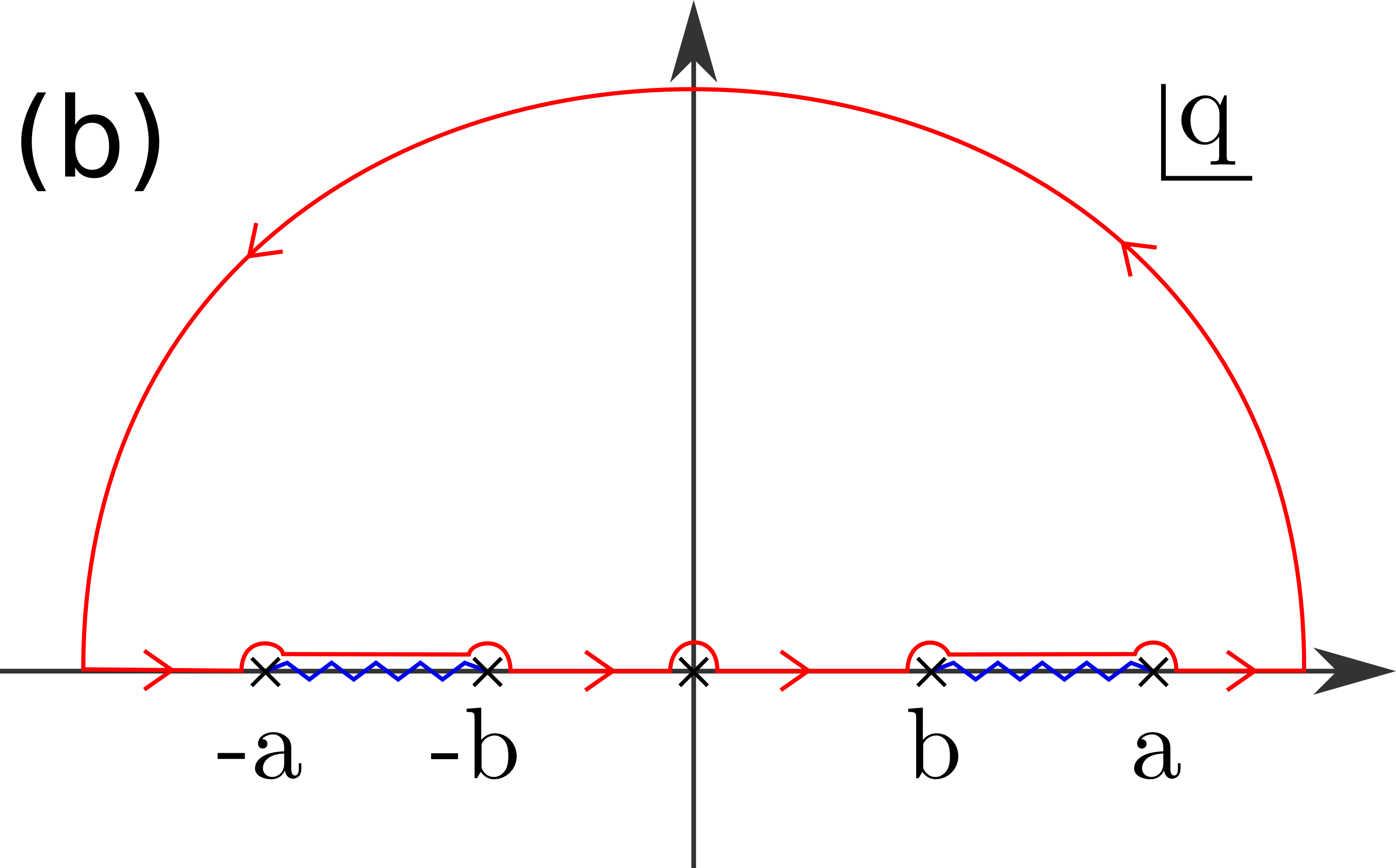
Supplementary Figure S5: (a) Scheme of the analytic structure of the integrand function of Eq. (S.A33), with two branch points $q=\pm a$ joined by a branch cut. (b) Scheme of the analytic structure of the integrand function of Eq. (LABEL:eq:Bintk2), with four branch points $q=\pm a$ and $q=\pm b$ joined by two branch cuts. The integration contour is drawn on red.

If we compute a similar integral to that of Eq. (S.A33), namely an integral where the modulus of the logarithm’s argument was dropped, let us call it $\widetilde{I}_{\sigma\sigma}(r)$, then we can show that it is equal to zero – the integral over the contour on the upper half complex plane vanishes when the contour is taken to infinity; thus the integral over the real axis is equal to zero. As we can write the logarithm of a given complex number $z$ as $\log z=log|z|+i\arg z$, then we can write

$$\log\bigg{[}\frac{2k_{F}^{\sigma}+q}{2k_{F}^{\sigma}-q}\bigg{]} = \left\{\begin{array}[]{ll}\log\bigg{[}\bigg{|}\frac{2k_{F}^{\sigma}+q}{2k_{F}^{\sigma}-q}\bigg{|}\bigg{]}&\textrm{, $|q|>a$,}\\ \\ \log\bigg{[}\bigg{|}\frac{2k_{F}^{\sigma}+q}{2k_{F}^{\sigma}-q}\bigg{|}\bigg{]}+i\pi&\textrm{, $|q|\leq a$,}\end{array}\right.\,,$$ (S.A37)

and thus Eq. (S.A33) becomes

$$I_{\sigma\sigma}(r) = \frac{m^{*}\Omega^{2}}{8r(2\pi)^{3}\hbar^{2}}\int_{-a}^{a}\textrm{d}q\,e^{iqr}\,\big{(}4{k_{F}^{\sigma}}^{2}-q^{2}\big{)}\,.$$ (S.A38)

which we can readily compute and obtain the expression in Eq. (S21).

Note that if we do not allow spin-flips of the hopping electrons, then we will only have the terms with $\zeta=\sigma$ in Eq. (LABEL:eq:H2nonfinal). In such a case, the exchange parameter expression will be given by $J(r_{\alpha\beta},k_{F}^{+},k_{F}^{-},\lambda_{\alpha},\lambda_{\beta})=J_{0}\mu_{0}^{2}\mu_{B}^{4}/(2\Omega^{2})\sum_{\sigma=\pm 1}t_{\sigma\sigma}^{(\alpha)}t_{\sigma\sigma}^{(\beta)}I_{\sigma\sigma}(r)$, which is going to result in the usual RKKY [refSupp]Ruderman_PR:1954-S,Kasuya_PTP:1956-S,Yosida_PR:1957-S expression for the indirect exchange parameter (if the amplitude for an hopping electron to have its spin unchanged when interacting with every nanoparticle equal unit, $t_{\sigma\sigma}^{(\alpha)}=t_{\sigma\sigma}^{(\beta)}=1$). The two terms for each spin direction arise from the fact that electrons with spin-up and spin-down may have different Fermi levels.

Computation of ’$I_{\sigma,-\sigma}(\mathbf{r}_{\alpha\beta})$’

Upon substituting $\mathbf{q}=\mathbf{k}-\mathbf{p}$ in Eq. (S22), we can write the sum in $\mathbf{k}$ (in the continuum limit) as

$$\widetilde{\mathcal{I}}_{\sigma}(\mathbf{q}) = -\frac{\Omega}{(2\pi)^{3}}\int\textrm{d}^{3}\mathbf{k}\frac{f_{\sigma}(\mathbf{k})-f_{-\sigma}(\mathbf{k}-\mathbf{q})}{E(\mathbf{k})-E(\mathbf{k}-\mathbf{q})-\Delta\mu_{\sigma,-\sigma}}\,,$$ (S.B39)

where, as before, $\Omega$ stands for the total volume of the crystal (with periodic boundary conditions).

Again we take the free electron gas approximation and define $\Delta_{\sigma}\equiv\Delta\mu_{\sigma,-\sigma}2m^{*}/\hbar^{2}=\big{(}k_{F}^{\sigma}\big{)}^{2}-\big{(}k_{F}^{-\sigma}\big{)}^{2}$, such that we can write the integral $\widetilde{\mathcal{I}}_{\sigma}(\mathbf{q})$ as

$$\widetilde{\mathcal{I}}_{\sigma}(\mathbf{q}) = \frac{2m^{*}\Omega}{(2\pi)^{3}\hbar^{2}}\int\textrm{d}^{3}\mathbf{k}\Bigg{(}\frac{f_{\sigma}(\mathbf{k})}{(\mathbf{k}-\mathbf{q})^{2}-\mathbf{k}^{2}+\Delta_{\sigma}}+\frac{f_{-\sigma}(\mathbf{k})}{(\mathbf{k}+\mathbf{q})^{2}-\mathbf{k}^{2}+\Delta_{-\sigma}}\Bigg{)}\equiv\widetilde{\mathcal{J}}_{\sigma}(\mathbf{q})+\widetilde{\mathcal{G}}_{\sigma}(\mathbf{q})\,,$$

where $\Delta_{-\sigma}=\big{(}k_{F}^{-\sigma}\big{)}^{2}-\big{(}k_{F}^{\sigma}\big{)}^{2}=-\Delta_{\sigma}$. And thus one can easily verify that $\widetilde{\mathcal{G}}_{\sigma}(\mathbf{q})=\widetilde{\mathcal{J}}_{-\sigma}(-\mathbf{q})$.

Let us first concentrate on $\widetilde{\mathcal{J}}_{\sigma}(\mathbf{q})$ and again assume that we are at zero temperature (see Appendix Tunable room-temperature ferromagnet using an iron-oxide and graphene oxide nanocomposite). Making the substitution $u=\cos\theta$ together with the following identification $\xi\equiv(q+\Delta/q)/(2k)$, we find that the Cauchy principal value of the integral in $\textrm{d}u$ reads $\log\big{[}\big{|}\big{(}q+\Delta_{\sigma}/q+2k\big{)}\big{(}q+\Delta_{\sigma}/q-2k\big{)}\big{|}\big{]}$. Computing the remaining integral (in d$k$) we obtain

$$\widetilde{\mathcal{J}}_{\sigma}(q) = \frac{m^{*}\Omega}{(2\pi)^{2}\hbar^{2}}\frac{k_{F}^{\sigma}}{2q}\bigg{(}q+\frac{\Delta_{\sigma}}{q}\bigg{)}\Bigg{(}1+\frac{4{k_{F}^{\sigma}}^{2}-\big{(}q+\Delta_{\sigma}/q\big{)}^{2}}{4k_{F}^{\sigma}\big{(}q+\Delta_{\sigma}/q\big{)}}\log\bigg{[}\bigg{|}\frac{2k_{F}^{\sigma}+\big{(}q+\Delta_{\sigma}/q\big{)}}{2k_{F}^{\sigma}-\big{(}q+\Delta_{\sigma}/q\big{)}}\bigg{|}\bigg{]}\Bigg{)}\,.$$

From the above equations it is simple to verify that $\widetilde{\mathcal{J}}_{\sigma}(-\mathbf{q})=\widetilde{\mathcal{J}}_{\sigma}(\mathbf{q})=\widetilde{\mathcal{J}}_{\sigma}(q)$ and $\widetilde{\mathcal{G}}_{\sigma}(\mathbf{q})=\widetilde{\mathcal{J}}_{-\sigma}(-\mathbf{q})$, and then conclude that the expression for $\widetilde{\mathcal{G}}_{\sigma}(\mathbf{q})$ is given by an analogous of Eq. (LABEL:eq:BappJ) where $\sigma\to-\sigma$ everywhere on the LHS.

We can identify $I_{\sigma,-\sigma}(r)=J_{\sigma,-\sigma}(r)+G_{\sigma,-\sigma}(r)$, where $J_{\sigma,-\sigma}(r)$ arises from the Fourier sum in $\mathbf{q}$ of $\widetilde{\mathcal{J}}_{\sigma}(q)$, while $G_{\sigma,-\sigma}(r)$ arises from the Fourier sum in $\mathbf{q}$ of $\widetilde{\mathcal{G}}_{\sigma}(q)$. Again, note that $G_{\sigma,-\sigma}(r)=J_{-\sigma,\sigma}(r)$. Taking the continuum limit of the Fourier sum in $\mathbf{q}$ of $\widetilde{\mathcal{J}}_{\sigma}(\mathbf{q})$ and doing the variable substitution $u=\cos\theta$ we obtain

$$J_{\sigma,-\sigma}(r) = \frac{m^{*}\Omega^{2}k_{F}^{\sigma}}{2ir(2\pi)^{4}\hbar^{2}}\int_{-\infty}^{\infty}\textrm{d}q\,e^{iqr}\,\bigg{(}q+\frac{\Delta_{\sigma}}{q}\bigg{)}\Bigg{(}1+\frac{4{k_{F}^{\sigma}}^{2}-\big{(}q+\Delta_{\sigma}/q\big{)}^{2}}{4k_{F}^{\sigma}\big{(}q+\Delta_{\sigma}/q\big{)}}\log\bigg{[}\bigg{|}\frac{2k_{F}^{\sigma}+\big{(}q+\Delta_{\sigma}/q\big{)}}{2k_{F}^{\sigma}-\big{(}q+\Delta_{\sigma}/q\big{)}}\bigg{|}\bigg{]}\Bigg{)}\,.$$

after using $\widetilde{\mathcal{J}}_{\sigma}(-q)=\widetilde{\mathcal{J}}_{\sigma}(q)$ and the expression in Eq. (LABEL:eq:BappJ).

The analytic structure of the integrand function in Eq. (LABEL:eq:Bintk2) is sketched in Supplementary Fig. S5(b): it has four branch points $q=\pm a$ and $q=\pm b$ which read $a=k_{F}^{\sigma}+\sqrt{{k_{F}^{\sigma}}^{2}-\Delta_{\sigma}}=k_{F}^{\sigma}+k_{F}^{-\sigma}$ and $b=k_{F}^{\sigma}-\sqrt{{k_{F}^{\sigma}}^{2}-\Delta_{\sigma}}=k_{F}^{\sigma}-k_{F}^{-\sigma}$. These four branch points are pairwise connected by a branch cut [see Supplementary Fig. S5(b)]. Additionally, there is a simple pole at $q=0$. In order to compute the integral in Eq. (LABEL:eq:Bintk2) we choose a contour as sketched in Supplementary Fig. S5(b) to do the integration.

Again we can make use of the trick used in Appendix Tunable room-temperature ferromagnet using an iron-oxide and graphene oxide nanocomposite: instead of computing the integral in Eq. (LABEL:eq:Bintk2), we start by computing a similar one, where the modulus of the logarithm’s argument was dropped; let us call it $\widetilde{J}_{\sigma,-\sigma}(r)$. Once more we can show that (the Cauchy principal value of) this integral is equal to zero, since the integral over the contour on the upper half complex plane vanishes when the contour is taken to infinity (as well as the contours around the pole and branch points). From the complex logarithm properties we can write

$$\log\bigg{[}\frac{(q+a)(q+b)}{(q-a)(q-b)}\bigg{]} = \left\{\begin{array}[]{ll}\log\bigg{[}\bigg{|}\frac{(q+a)(q+b)}{(q-a)(q-b)}\bigg{|}\bigg{]}&\textrm{, $|q|>a\land|q|<b$,}\\ \\ \log\bigg{[}\bigg{|}\frac{(q+a)(q+b)}{(q-a)(q-b)}\bigg{|}\bigg{]}+i\pi&\textrm{, $-a\leq q\leq-b\land b\leq q\leq a$,}\end{array}\right.\,,$$ (S.B46)

where we have used the expressions for $a$ and $b$ to rewrite the argument of the logarithm in Eq. (LABEL:eq:Bintk2) in the left hand side of the above equation. With this equality we can write $J_{\sigma,-\sigma}(r)$

$$J_{\sigma,-\sigma}(r) = \frac{m^{*}\Omega^{2}}{16r(2\pi)^{3}\hbar^{2}}\Bigg{\{}\int_{-a}^{-b}\textrm{d}q\,e^{iqr}\,\bigg{[}4\big{(}k_{F}^{\sigma}\big{)}^{2}-\bigg{(}q+\frac{\Delta_{\sigma}}{q}\bigg{)}^{2}\bigg{]}+\int_{b}^{a}\textrm{d}q\,e^{iqr}\,\bigg{[}4\big{(}k_{F}^{\sigma}\big{)}^{2}-\bigg{(}q+\frac{\Delta_{\sigma}}{q}\bigg{)}^{2}\bigg{]}\Bigg{\}}\,,$$

(S.B47)

while $G_{\sigma,-\sigma}(r)$ is obtained from substituting $\sigma\to-\sigma$ on the LHS of Eq. (S.B47).

Finally, we can show that computing the above integrals and summing the $J_{\sigma,-\sigma}(r)$ and the $G_{\sigma,-\sigma}(r)$ [remember that $I_{\sigma,-\sigma}(r)=J_{\sigma,-\sigma}(r)+G_{\sigma,-\sigma}(r)$] we obtain the result stated in Eq. (S23). From it is straightforward to verify that $I_{-\sigma,\sigma}(r)=I_{\sigma,-\sigma}(r)$, as it should be since $G_{\sigma,-\sigma}(r)=J_{-\sigma,\sigma}(r)$ and $I_{\sigma,-\sigma}(r)=J_{\sigma,-\sigma}(r)+G_{\sigma,-\sigma}(r)=J_{\sigma,-\sigma}(r)+J_{-\sigma,\sigma}(r)$.

References

- [1] Slonczewski, J. “Current-driven excitation of magnetic multilayers”, J. Magn. Magn. Mater. 159, L1 – L7 (1996).
- [2] Berger, L. “Emission of spin waves by a magnetic multilayer traversed by a current”, Phys. Rev. B 54, 9353–9358 (1996).
- [3] Ralph, D. & Stiles, M. “Spin transfer torques”, J. Magn. Magn. Mater. 320, 1190 – 1216 (2008).
- [4] Fiebig, M. “Revival of the magnetoelectric effect”, J. Phys. D: Appl. Phys. 38, R123 (2005).
- [5] Eerenstein, W., Mathur, N. D. & Scott, J. F. “Multiferroic and magnetoelectric materials”, Nature 442, 759 – 765 (2006).
- [6] Vaz, C. A. F. “Electric field control of magnetism in multiferroic heterostructures”, J. Phys.: Condens. Matter 24, 333201 (2012).
- [7] Weisheit, M. et al. “Electric field-induced modification of magnetism in thin-film ferromagnets”, Science 315, 349–351 (2007).
- [8] Chiba, D. et al. “Electrical control of the ferromagnetic phase transition in cobalt at room temperature”, Nat. Mater. 10, 853 – 856 (2011).
- [9] Chiba, D. & Ono, T. “Control of magnetism in co by an electric field”, J. Phys. D: Appl. Phys. 46, 213001 (2013).
- [10] Su, C. et al. “Probing the catalytic activity of porous graphene oxide and the origin of this behaviour”, Nat. Commun. 3, 1298 (2012).
- [11] Lin, A. L. et al. “Room temperature magnetic graphene oxide- iron oxide nanocomposite based magnetoresistive random access memory devices via spin-dependent trapping of electrons”, Small 10, 1945–1952 (2014).
- [12] Ruderman, M. A. & Kittel, C. “Indirect exchange coupling of nuclear magnetic moments by conduction electrons”, Phys. Rev. 96, 99–102 (1954).
- [13] Kasuya, T. “A theory of metallic ferro- and antiferromagnetism on zener’s model”, Prog. Theo. Phys. 16, 45–57 (1956).
- [14] Yosida, K. “Magnetic properties of cu-mn alloys”, Phys. Rev. 106, 893–898 (1957).
- [15] Baibich, M. N. et al. “Giant magnetoresistance of (001)fe/(001)cr magnetic superlattices”, Phys. Rev. Lett. 61, 2472–2475 (1988).
- [16] Binasch, G., Grünberg, P., Saurenbach, F. & Zinn, W. “Enhanced magnetoresistance in layered magnetic structures with antiferromagnetic interlayer exchange”, Phys. Rev. B 39, 4828–4830 (1989).
- [17] Jiang, H. W., Johnson, C. E. & Wang, K. L. “Giant negative magnetoresistance of a degenerate two-dimensional electron gas in the variable-range-hopping regime”, Phys. Rev. B 46, 12830–12833 (1992).
- [18] Ioffe, L. & Spivak, B. “Giant magnetoresistance in the variable-range hopping regime”, J. Exp. Theor. Phys. 117, 551–569 (2013).
- [19] De Gennes, P.G. “Polarisation de charge (ou de spin) au voisinage d’une impureté dans un alliage”, J. Phys. Radium 23, 630–636 (1962).
- [20] Lerner, I. V. “Dependence of the ruderman-kittel-kasuya-yosida interaction on nonmagnetic disorder”, Phys. Rev. B 48, 9462–9477 (1993).
- [21] Sobota, J. A., Tanasković, D. & Dobrosavljević, V. “Rkky interactions in the regime of strong localization”, Phys. Rev. B 76, 245106 (2007).
- [22] Metropolis, N., Rosenbluth, A. W., Rosenbluth, M. N., Teller, A. H. & Teller, E. “Equation of state calculations by fast computing machines”, J. Chem. Phys. 21, 1087–1092 (1953).
- [23] Wolff, U. “Collective monte carlo updating for spin systems”, Phys. Rev. Lett. 62, 361–364 (1989).
Supplementary Information

References

- [1] Fleetwood, D. M. et al. “Effects of oxide traps, interface traps, and ’border traps’ on metal-oxide-semiconductor devices”, J. Appl. Phys. 73, 5058–5074 (1993).
- [2] McCarthy, K. T., Hebard, A. F. & Arnason, S. B. “Magnetocapacitance: Probe of spin-dependent potentials”, Phys. Rev. Lett. 90, 117201 (2003).
- [3] Lin, A. L., Wu, T., Chen, W. & Wee, A. T. S. “Room temperature positive magnetoresistance via charge trapping in polyaniline-iron oxide nanoparticle composites”, Appl. Phys. Lett. 103 (2013).
- [4] Zhu, J. et al. “Magnetic field induced capacitance enhancement in graphene and magnetic graphene nanocomposites”, Energy Environ. Sci. 6, 194–204 (2013).
- [5] Mott, N. F. “Conduction in non-crystalline materials”, Philos. Mag. 19, 835–852 (1969).
- [6] De Gennes, P.G. “Polarisation de charge (ou de spin) au voisinage d’une impureté dans un alliage”, J. Phys. Radium 23, 630–636 (1962).
- [7] Lerner, I. V. “Dependence of the ruderman-kittel-kasuya-yosida interaction on nonmagnetic disorder”, Phys. Rev. B 48, 9462–9477 (1993).
- [8] Sobota, J. A., Tanasković, D. & Dobrosavljević, V. “Rkky interactions in the regime of strong localization”, Phys. Rev. B 76, 245106 (2007).
- [9] Ruderman, M. A. & Kittel, C. “Indirect exchange coupling of nuclear magnetic moments by conduction electrons”, Phys. Rev. 96, 99–102 (1954).
- [10] Kasuya, T. “A theory of metallic ferro- and antiferromagnetism on zener’s model”, Prog. Theo. Phys. 16, 45–57 (1956).
- [11] Yosida, K. “Magnetic properties of cu-mn alloys”, Phys. Rev. 106, 893–898 (1957).
- [12] Fullenbaum, M. S. & Falk, D. S. “Electron spin polarization due to a magnetic impurity”, Phys. Rev. 157, 452–456 (1967).
- [13] Kim, J. G., Lee, E. K. & Lee, S. “Temperature-dependent ruderman-kittel-kasuya-yosida interaction”, Phys. Rev. B 51, 670–673 (1995).
- [14] Kim, J. G., Choi, Y.-H. S., Lee, E. K. & Lee, S. “Temperature-dependent free-electron susceptibility for one, two, and three dimensions”, Phys. Rev. B 59, 3661–3670 (1999).
- [15] Wolff, U. “Collective monte carlo updating for spin systems”, Phys. Rev. Lett. 62, 361–364 (1989).
- [16] Metropolis, N., Rosenbluth, A. W., Rosenbluth, M. N., Teller, A. H. & Teller, E. “Equation of state calculations by fast computing machines”, J. Chem. Phys. 21, 1087–1092 (1953).
- [17] Lin, A. L. et al. “Room temperature magnetic graphene oxide- iron oxide nanocomposite based magnetoresistive random access memory devices via spin-dependent trapping of electrons”, Small 10, 1945–1952 (2014).