Monte Carlo Simulations of Lattice Models for Single Polymer Systems

Abstract

Single linear polymer chains in dilute solutions under good solvent conditions are studied by Monte Carlo simulations with the pruned-enriched Rosenbluth method up to the chain length $N\sim{\cal O}(10^{4})$. Based on the standard simple cubic lattice model (SCLM) with fixed bond length and the bond fluctuation model (BFM) with bond lengths in a range between $2$ and $\sqrt{10}$, we investigate the conformations of polymer chains described by self-avoiding walks (SAWs) on the simple cubic lattice, and by random walks (RWs) and non-reversible random walks (NRRWs) in the absence of excluded volume (EV) interactions. In addition to flexible chains, we also extend our study to semiflexible chains for different stiffness controlled by a bending potential. The persistence lengths of chains extracted from the orientational correlations are estimated for all cases. We show that chains based on the BFM are more flexible than those based on the SCLM for a fixed bending energy. The microscopic differences between these two lattice models are discussed and the theoretical predictions of scaling laws given in the literature are checked and verified. Our simulations clarify that a different mapping ratio between the coarse-grained models and the atomistically realistic description of polymers is required in a coarse-graining approach due to the different crossovers to the asymptotic behavior.

I Introduction

In the theoretical study of polymer physics Flory1969 ; deGennes1979 , computer simulations provide a powerful method to mimic the behavior of polymers covering the range from atomic to coarse-grained scales depending on the problems one is interested in Binder1995 ; Binder2008 . The generic scaling properties of single linear and branched polymers in the bulk or confinement under various solvent conditions have been described quite well by simple coarse-grained lattice models (i.e., random walks (RWs), non-reversible random walks (NRRWs), self-avoiding random walks (SAWs), or interacting self-avoiding random walks (ISAWs) on a regular lattice, regarding the interactions between non-bonded monomers). As an alternative one can use coarse-grained models in the continuum, such as a bead-spring model (BSM) (where all beads interact with a truncated and shifted Lennard-Jones (LJ) potential while the bonded interactions are captured by a finitely extensible nonlinear elastic (FENE) potential) using Monte Carlo and molecular dynamics simulations Binder1995 . On the one hand, however, as the size and complexity of a system increases, detailed information at the atomic scale may be lost when employing low resolution coarse-graining representations. On the other hand, the cost of computing time may be too high if the system is described at high resolution. Therefore, more scientific effort has been devoted to developing an appropriate coarse-grained model which can reproduce the global thermodynamic properties and the local mechanical and chemical properties such as the intermolecular forces between polymer chains Murat1998 ; Plathe2002 ; Harman2006 ; Harman2007 ; Gujrati2010 ; Vettorel2010 ; Zhang2013 . While these models are already known since a long time, the present work is the first study presenting precise data on conformational properties of these model, when a bond angle potential is included.

In this paper we deal with linear polymer chains in dilute solutions under good solvent conditions, and describe them by lattice models on the simple cubic lattice. Although coarse-grained lattice models neglect the chemical detail of a specific polymer chain and only keep chain connectivity (topology) and excluded volume, the universal behavior of polymers still remains the same in the thermodynamic limit (as the chain length $N\rightarrow\infty$) deGennes1979 , Two coarse-grained lattice models, the standard simple cubic lattice model (SCLM) and the bond fluctuation model (BFM) Binder1995 ; Carmesin1988 ; Deutsch1991 ; Paul1991 ; Mueller2005 , are considered for our simulations. The SCLM is often used for the test of new simulation algorithms, and the verification of theoretically predicted scaling laws due to its simplicity and computational efficiency. The BFM has the advantages that the computational efficiency of lattice models is kept and the behavior of polymers in a continuum space can be described approximately. The model thus introduces some local conformational flexibility while retaining the computational efficiency of lattice models for implementing excluded volume interactions by enforcing a single occupation of each lattice vertex.

redThe excluded volume effect plays an essential role in any real polymer chain, while in a dilute solution under a theta solvent condition, or in concentrated polymer solutions such as melts, and glasses, the real polymer chain behaves like an ideal chain. The excluded volume constraint can easily be incorporated in the lattice models by simply forbidding any two effective monomers occupying the same lattice site (cell). Tries et al. have successfully mapped linear polyethylene in the melt onto the BFM and their results are in good agreement with experimental viscosimetric results quantitatively without adjusting any extra parameters Mueller2005 ; Tries1997 . Varying the backbone length and side chain length of the bottle-brush polymer based on the BFM, a direct comparison of the structure factors between the experimental data for the synthetic bottle-brush polymer consisting of hydroxyethyl methacrylate (PMMA) as the backbone polymer and flexible poly(n-butyl acrylate) (PnBA) as side chains in a good solvent (toluene) and the Monte Carlo results is given Hsu2009 . Furthermore, the lattice models have also been used widely to investigate the conformational properties of protein-folding Lau1989 and DNA in chromosomes Vettorel2009a ; Vettorel2009b ; Halverson2014 in biopolymers. For alkane-like chains the angles between subsequent effective bonds are not continuously distributed, but only discrete angles are allowed. Therefore, the lattice model such as the SCLM where only the discrete angles $0^{o}$ and $90^{o}$ are allowed is an ideal model for studying alkane-like chains of different stiffnesses.

A direct comparison of simulation results between the lattice models and the off-lattice BSM is also possible, e.g. linear polymers Wittmer2007 and ring polymers Halverson2013 in a melt, adsorption of multi-block and random copolymers Bhattacharya2008 , semiflexible chains under a good solvent condition Huang2014c , the crossover from semiflexible polymer brushes towards semiflexible mushrooms as the grafting density decreases Egorov2014 . Results from these two coarse-grained models are qualitatively the same. Namely, they both show the same scaling behavior, but the amplitudes and the critical or the crossover points can vary depending on the underlying models. However, our main motivation was to understand the microscopic differences between the two lattice models, SCLM and BFM, for describing the conformations of polymers and to provide this information for the further development of a multi-scale approach for studying polymers of complex topology and polymer solutions at high concentration based on the lattice models. Therefore, we only focus on the two coarse-grained lattice models, SCLM and BFM, here. In the mapping between atomistic and coarse-grained models, it turns out that a bond angle potential also needs to be included in the coarse-grained models, as is done here.

The outline of the paper is as follows: Sec. II describes the models and the simulation technique. Sec. III and Sec. IV review the properties of flexible chains and semiflexible chains, respectively. Polymer chains described by SAWs, and by RWs and NRRWs in the absence of excluded volume effects are studied and compared with theoretical predictions. Finally our conclusions are summarized in Sec. V.

II Models and simulation methods

The basic characteristics of linear polymer chains depend on the solvent conditions. Under good solvent conditions the repulsive interactions (the excluded volume effect) and entropic effects dominate the conformation, and the polymer chain tends to swell to a random coil. In the thermodynamic limit, namely the chain length $N\rightarrow\infty$, the partition function scales as

$$Z_{N}\sim\mu_{\infty}^{-N}N^{\gamma_{d}-1}\sim q_{\rm eff}^{N}N^{\gamma_{d}-1}$$ (1)

where $\mu_{\infty}$ is the critical fugacity per monomer, $q_{\rm eff}$ is the effective coordination number, and $\gamma$ is the entropic exponent related to the topology. In two dimensions deGennes1979 $\gamma=43/32$, while the best estimate Hsu2004 for $d=3$ is $\gamma=1.1573(2)$. For the standard self-avoiding walks on the simple cubic lattice Grassberger2005 in $d=3$ one has $\mu_{\infty}=0.21349098(5)$ and the corresponding effective coordination number $q_{\rm eff}=1/\mu_{\infty}=4.6840386(11)$. The conformations of polymer chains characterized by the mean square end-to-end distance, $\langle R_{e}^{2}\rangle$, and the mean square gyration radius, $\langle R_{g}^{2}\rangle$, scale as Li1995 ; Nickel1991 :

$$\langle R_{e}^{2}\rangle/\ell_{b}^{2}=A_{e}N^{2\nu}[1+{\cal O}(N^{-\Delta})]\,,$$ (2)

and

$$\langle R_{g}^{2}\rangle/\ell_{b}^{2}=A_{g}N^{2\nu}[1+{\cal O}(N^{-\Delta})]$$ (3)

where $\nu$ is the Flory exponent, $\Delta$ is the leading correction to the scaling exponent, $A_{e}$ and $A_{g}$ are non-universal constants, and $\ell_{b}^{2}$ is the mean square bond length. The quantities $\nu$, $\Delta$, and the ratio $A_{e}/A_{g}$ are universal Privman1991 , while the quantities, $A_{e}$, $A_{g}$, $\ell_{b}$, and $q_{\rm eff}$, depend on the microscopic realization. In $d=2$ one has $\nu_{2}=3/4$, while in $d=3$ the most accurate estimate of the Flory exponent Clisby2010 $\nu=0.587597(7)$. We use $\nu=0.5876$ for our data analysis in this paper.

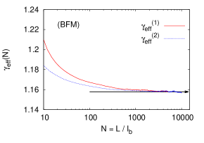
(a)      (b)

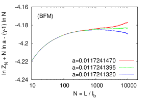
Figure 1: (a) Effective exponents $\gamma_{\rm eff}^{(1)}$ and $\gamma_{\rm eff}^{(2)}$ [computed from Eqs. (5) and (6) ] plotted versus $N$ on a semi-log scale. $\gamma=\lim_{N\rightarrow\infty}\gamma_{\rm eff}^{(1)}(N)=\lim_{N\rightarrow\infty}\gamma_{\rm eff}^{(2)}(N)=1.1578(6)$. (b) $\ln Z_{N}+N\ln a-(\gamma-1)\ln N$ with $\gamma=1.1578$ determined from (a) plotted versus $N$ on a semi-log scale. The best estimate of fugacity $\mu=a=0.0117241395(75)$ is determined by the horizontal curve.

Two models are used for simulating linear polymers in the bulk under good solvent conditions. One is the standard SAW on the simple cubic lattice, effective monomers being described by occupied lattice sites, connected by bonds of fixed length $\mid\vec{b}\mid=\ell_{b}=1$. Each site can be visited only once, and thus the excluded volume interaction is realized. The other is the standard bond fluctuation model (BFM). On the simple cubic lattice each effective monomer of a SAW chain blocks all eight corners of an elementary cube of the lattice from further occupation. Two successive monomers along a chain are connected by a bond vector $\vec{b}$ which is taken from the set {$(\pm 2,0,0)$,$(\pm 2,\pm 1,0)$, $(\pm 2,\pm 1,\pm 1)$, $(\pm 2,\pm 2,\pm 1)$, $(\pm 3,0,0)$, $(\pm 3,\pm 1,0)$} including also all permutations. The bond length $\ell_{b}$ is therefore in a range between $2$ and $\sqrt{10}$. There are in total $108$ bond vectors and $87$ different bond angles between two sequential bonds along a chain serving as candidates for building the conformational structure of polymers. The partition sum of a SAW of $N$ steps is

$$Z_{N}=\sum_{\rm config.}1$$ (4)

which is simply the total number of possible configurations consisting of $(N+1)$ monomers.

In the literature there are still no estimates of the fugacity $\mu_{\infty}(=1/q_{\rm eff})$ and the entropic exponent $\gamma$ for SAWs on the BFM. According to the scaling law of the partition sum $Z_{N}$, Eq. (1), the effective entropic exponent $\gamma_{\rm eff}^{(1)}$ obtained from triple ratios Grassberger1997b

$$\gamma_{\rm eff}^{(1)}(N)=1+\frac{7\ln Z_{N}-6\ln Z_{N/3}-\ln Z_{5N}}{\ln(3^{6}/5)}$$ (5)

is shown in Fig. 1a. It gives $\gamma=\lim_{N\rightarrow\infty}\gamma_{\rm eff}^{(1)}(N)=1.1578(6)$. The fugacity $\mu_{\infty}$ is therefore determined by adjusting the value $a$ such that the curve of ${\ln Z_{N}+N\ln a-(\gamma-1)\ln N}$ with $\gamma=1.1578$ becomes horizontal for very large $N$ (see Fig. 1b). We obtain the fugacity ${\mu_{\infty}=0.0117241395(75)}$ and the corresponding effective coordination number ${q_{\rm eff}=85.294106(55)}$ listed in Table 1. In Fig. 1a we also show the asymptotic behavior of the effective entropic exponent $\gamma_{\rm eff}^{(2)}$ defined by

$$\gamma_{\rm eff}^{(2)}(N)=1+\frac{\ln\left[\mu^{3N/2}Z(2N)/Z(N/2)\right]}{\ln 4}$$ (6)

with our estimate of $\mu_{\infty}$ for comparison.

If the excluded volume effect is ignored completely, a polymer chain behaves as an ideal chain. It is well described by a random walk (RW), a walk that can cross itself or may trace back the same path, or by a non-reversal random walk (NRRW) where immediate back tracing is not allowed. The partition sums of RW and NRRW are given by

$$Z_{N}=q^{N}\quad{\rm(RW)}\,,\quad Z_{N}=q(q-1)^{N-1}\quad{\rm(NRRW)}$$ (7)

where $q$ is the coordination number. $q=6$ for the standard RW on the simple cubic lattice, and $q=108$ for the BFM Kremer1988 . The Flory exponent is $\nu=1/2$ for an ideal chain and its mean square gyration radius $\langle R_{g}^{2}\rangle=\langle R_{e}^{2}\rangle/6$.

For the simulations of single RW, NRRW, and SAW chains we use the pruned-enriched Rosenbluth method (PERM) Grassberger1997 . It is a biased chain growth algorithm with resampling and population control. In this algorithm a polymer chain is built like a random walk by adding one monomer at each step with a bias depending on the problem at hand, and each configuration carries its own weight. The population control at each step is made such that the “bad” configurations are pruned with a certain probability, and the “good” configurations are enriched by properly reweighting, until a chain has either grown to the maximum length of steps, $N$, or has been killed due to attrition. A detailed description of the algorithm PERM and its applications is given in a review paper HsuR2011 . The algorithm has the advantage that the partition sum can be estimated very precisely and directly. It is also very efficient for simulating linear polymer chains up to very long chain lengths in dilute solution at and above the $\Theta$-point. Therefore, we apply the algorithm on the two lattice models, SCLM and BFM, in order to check for major differences between these two microscopic models. The longest chain length is $N=50000$ in our simulations here.

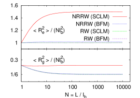
(a)      (b)

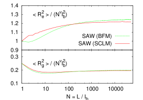
Figure 2: Mean square end-to-end distance $\langle R^{2}_{e}\rangle$ and gyration radius $\langle R^{2}_{g}\rangle$ scaled by $(N^{\nu}\ell_{b}^{2})$ with the Flory exponent $\nu=1/2$ for RWs and NRRWs (a), and $\nu=0.5876$ for SAWs Clisby2010 , plotted against $N$. Here the bond length $\ell_{b}=\langle\vec{b}^{2}\rangle^{1/2}$: $\ell_{b}=1$ (SCLM) and $\ell_{b}=2.72$ (BFM).

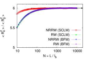
(a) (b)

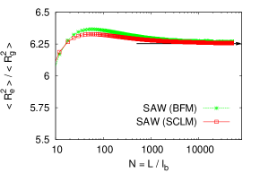
Figure 3: Ratio between the mean square end-to-end distance and the mean square gyration radius, $\langle R^{2}_{e}\rangle/\langle R^{2}_{g}\rangle$, plotted against the chain segments $N$, for RWs and NRRWs (a), and for SAWs (b). As $N\gg 0$, $\langle R_{e}^{2}\rangle/\langle R_{g}^{2}\rangle\sim 6.00$ in (a) and $\langle R_{e}^{2}\rangle/\langle R_{g}^{2}\rangle\sim 6.25$ in (b).

Table 1: The estimates of fugacity $\mu_{\infty}$, the effective coordination number $q_{\rm eff}$ in Eq. (1), the amplitudes $A_{e}$ and $A_{g}$ in Eqs. (2) and (3) determined from the simulation data of $\langle R_{e}^{2}\rangle$ and $\langle R_{g}^{2}\rangle$ for RWs, NRRWs, and SAWs based on the two lattice models, SCLM and BFM.

	SCLM			BFM
model	RW	NRRW	SAW	RW	NRRW	SAW
$\mu_{\infty}$	1/6	1/5	0.21349098(5) Grassberger2005	1/108	1/107	0.01172414395(75)
$q_{\rm eff}$	6	5	4.6840386(11)	108	107	85.294106(55)
$A_{e}$	1.0000(2)	1.4988(4)	1.220(3)	0.9986(2)	1.0714(2)	1.247(5)
$A_{g}$	0.16666(0)	0.24985(7)	0.1952(4)	0.16645(4)	0.16959(3)	0.1993(6)

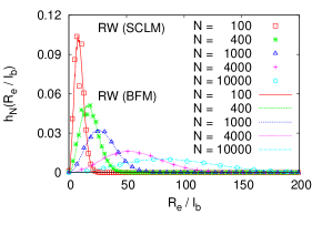
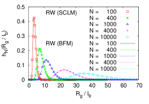
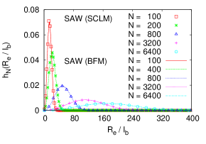
(a)      (b) (c)      (d)

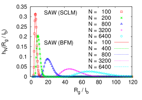
Figure 4: (a),(c) Normalized probability distributions of end-to-end distance, $h_{N}(R_{e}/\ell_{b})(={\cal P}(R_{e}/\ell_{b}))$, plotted versus $R_{e}/\ell_{b}$. (b),(d) similar as (a),(c), but for gyration radius $R_{g}$. Data are for RWs (a),(b) and SAWs (c),(d). Several values of chain lengths $N$ are chosen, as indicated.

III Conformations of single linear polymer chains: RWs, NRRWs, and SAWs

We employ the pruned-enriched Rosenbluth method (PERM) for the simulations of long single linear polymer chains of chain lengths (segments) up to $N\sim{\cal O}(10^{4})$, modeled by RWs, NRRWs, and SAWs depending on the interactions between monomers. Figure 2a with $\nu=1/2$ and Fig.2b with $\nu=0.5876$ show that the scaling laws, Eqs. (2) and (3), are verified as one should expect. The mean square end-to-end distance simply is

$$\langle R_{e}^{2}\rangle=\langle(\vec{r}_{N}-\vec{r}_{0})^{2}\rangle=\left\langle\left(\sum_{j=1}^{N}\vec{b}_{j}\right)^{2}\right\rangle\,.$$ (8)

The mean square gyration radius is given by

$$\langle R_{g}^{2}\rangle = \frac{1}{N+1}\left\langle\sum_{j=0}^{N}(\vec{r}_{j}-\vec{r}_{CM})^{2}\right\rangle$$ (9)

$$= \frac{1}{(N+1)^{2}}\left\langle\sum_{j=0}^{N}\sum_{k=0}^{N}(\vec{r}_{j}-\vec{r}_{k})^{2}\right\rangle\,,$$

where $\vec{r}_{CM}=\sum_{j=0}^{N}\vec{r}_{j}/(N+1)$ is the center of mass position of the polymer. The amplitudes $A_{e}$ and $A_{g}$ for RWs, NRRWs, SAWs based on the two lattice models, SCLM and BFM, are listed in Table 1. Results of $\langle R_{e}^{2}\rangle/(N\ell_{b}^{2})$ and $\langle R_{g}^{2}\rangle/(N\ell_{b}^{2})$ for RWs from both models follow the same curves although the bond vectors in the BFM are not all along the lattice directions and do not have the same bond length. Here $\ell_{b}$ is the root-mean square bond length, $\ell_{b}=1$ for the SCLM and $\ell_{b}=2.72$ for the BFM. In Fig. 2a, values of $\langle R_{e}^{2}\rangle/(N\ell_{b}^{2})$ and $\langle R_{g}^{2}\rangle/(N\ell_{b}^{2})$ for NRRWs, obtained from SCLM for all lengths $N$ are significant larger than that obtained from the BFM, since at each step the walker can only go straight or make a $90^{o}$ L-turn in the SCLM. In Fig. 2b, the two curves showing the results of $\langle R_{e}^{2}\rangle/(N^{\nu}\ell_{b}^{2})$ [$\langle R_{g}^{2}\rangle/(N^{\nu}\ell_{b}^{2})$] with $\nu=0.5876$ as functions of $N$ obtained from the two models intersect at $N\approx 180$, and finally the amplitude for BFM is larger in the asymptotic regime. The slight deviation from the plateau value is due to the finite size effects. The correction exponent $\Delta$ [Eqs. (2) and (3)] for these two models is determined by plotting $\langle R_{e}^{2}\rangle/N^{2\nu}$ and $\langle R_{g}^{2}\rangle/N^{2\nu}$ versus $x\equiv N^{-\delta}$ (not shown). One should expect straight lines near $x=0$ if and only if $\delta=\Delta$. We obtain $\Delta=0.48(5)$ for both models, which is in agreement with the previous simulation in Ref. Li1995 ; Grassberger1997b ; Clisby2010 within error bars. The ratio between the mean square end-to-end distance and the mean square gyration radius, is indeed $\langle R_{e}^{2}\rangle/\langle R_{g}^{2}\rangle\approx 6.000(3)$ for RWs and NRRWs (Fig. 3a). For SAWs our results give $\langle R_{e}^{2}\rangle/\langle R_{g}^{2}\rangle=6.25(2)$ (Fig. 3b). For SAWs on the simple cubic lattice the most accurate estimates of $A_{e}=1.22035(25)$, $A_{g}=0.19514(4)$, and $A_{e}/A_{g}=6.2537(26)$ are given in Ref. Clisby2010 . Our results are also in perfect agreement with them. However, much longer chain lengths will be needed for a more precise estimate of the plateau value of the ratio in the asymptotic scaling regime. Note that for $10<N<100$ the behavior is clearly model-dependent.

We include here the RW and NRRW versions of both models not just for the sake of an exercise: often the mapping from an atomistic to a coarse-grained model is to be done under melt conditions, where excluded volume interactions are screened.

The shapes of polymer chains can also be described by the probability distributions of end-to-end distance and gyration radius, $P(R_{e}/\ell_{b})$ and $P(R_{g}/\ell_{b})$, respectively. Numerically, they are obtained by accumulating the histogram $H_{N}(x)$ of $x$ over all configurations of length $N$, given by

$$H_{N}(x)=\sum_{\rm configs.}W_{N}(x^{\prime})\delta_{x,x^{\prime}}\,,$$ (10)

here each configuration carries its own weight $W_{N}(x^{\prime})$. The normalized histogram is therefore,

$$h_{N}(x)=H_{N}(x)/\sum_{x^{\prime}}H_{N}(x^{\prime})\,.$$ (11)

Results of $h_{N}(R_{e}/\ell_{b})$ and $h_{N}(R_{g}/\ell_{b})$ for RWs and SAWs obtained from the two models for various values of chain lengths $N$ are shown in Fig. 4. We see that both models give for $N>100$ the same distributions of $R_{e}/\ell_{b}$ and $R_{g}/\ell_{b}$ although the mean values of $R_{e}/\ell_{b}$ and $R_{g}/\ell_{b}$ are slightly different between these two lattice models (Fig. 2b) for SAWs. Note that an angular average over all directions has been included in the accumulating process of the histogram due to spherical symmetry. Thus, the normalized histograms of $R_{e}/\ell_{b}$,

$$h_{N}\left(R_{e}/\ell_{b}\right)={\cal P}_{N}({R_{e}}/{\ell_{b}})=4\pi C_{e,N}\left({R_{e}}/{\ell_{b}}\right)^{2}P_{N}\left({\vec{R}_{e}}/{\ell_{b}}\right)\,,$$ (12)

with

$$\int_{0}^{\infty}{\cal P}_{N}({R_{e}}/{\ell_{b}})d\left(R_{e}/\ell_{b}\right)=1\,,$$ (13)

and the normalized histograms of $R_{g}/\ell_{b}$,

$$h_{N}\left(R_{g}/\ell_{b}\right)={\cal P}_{N}({R_{g}}/{\ell_{b}})=4\pi C_{g,N}\left({R_{g}}/{\ell_{b}}\right)^{2}P_{N}\left({R_{g}}/{\ell_{b}}\right)\,,$$ (14)

with

$$\int_{0}^{\infty}{\cal P}_{N}({R_{g}}/{\ell_{b}})d\left(R_{g}/\ell_{b}\right)=1\,,$$ (15)

where $C_{e,N}$ and $C_{g,N}$ are the normalization factors.

The probability distribution of end-to-end distance for ideal chains is simply a Gaussian distribution,

$$P(\vec{R_{e}}/\ell_{b})=\frac{1}{(2\pi N/3)^{3/2}}\exp(-\frac{3(R_{e}/\ell_{b})^{2}}{2N})\,.$$ (16)

Our numerical data for RWs obtained from BFM and SCLM shown in Fig. 4 are in perfect agreement with the Gaussian distribution (see Fig. 5). From Eqs. (16), (12) and (13) we obtain the normalized factor $C_{e,N}=1$.

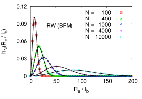
Figure 5: Same as in Fig. 4a, but data are only for BFM. The predicted distribution $4\pi(R_{e}/\ell_{b})^{2}P(R_{e}/\ell_{b})$ for various values of $N$ are shown by solid curves. Here the distribution function $P(R_{e}/\ell_{b})$ is given by Eq. (16).

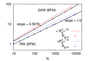
Figure 6: Root mean square radius of gyration, $\langle R_{g}^{2}\rangle^{1/2}$, and the gyration radius $R_{g,m}$ where $P(R_{g})$ has its maximum value, plotted against chain length $N$ for RWs and SAWs. Data are for BFM.

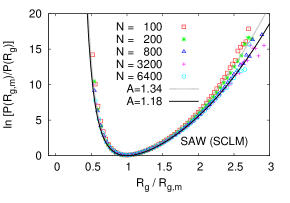
(a)      (b)

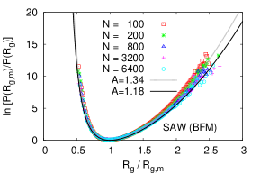
Figure 7: Logarithm of the rescaled probability distribution of gyration radius, $\ln(P(R_{g,m})/P(R_{g}))$ as a function of $R_{g}/R_{g,m}$ for SAWs obtained from the models (a) SCLM and (b) BFM. The best fit of Eq. (19) with $A=1.18$ to our data is shown by the solid curve. The dashed curve with $A=1.34$ given in Ref. Bishop1991 is also shown for the comparison. Several values of chain lengths $N$ are chosen, as indicated.

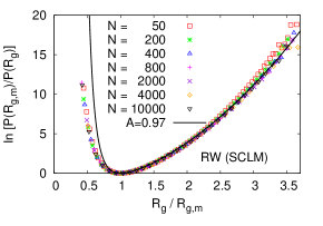
(a)      (b)

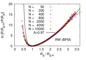
Figure 8: Similar as in Fig. 7, but for RWs. The best fitting of our data gives $A=0.97$ for both models.

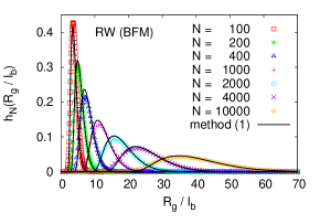
(a)      (b)

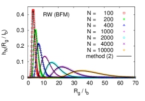
Figure 9: Normalized probability distributions of $R_{g}/\ell_{b}$, $h(R_{g}/\ell_{b})={\cal P}_{N}(R_{g}/\ell_{b})$, plotted versus $R_{g}/\ell_{b}$ for various values of $N$, and for BFM. The fitting functions $4\pi C_{g,N}(R_{g}/\ell_{b})^{2}P(R_{g}/\ell_{b})$ [Eqs. (14), (15), and (17)] with parameters $a_{1}$, $a_{2}$, and $C_{g,N}$ determined by method (1) and method (2) are shown by curves for comparison in (a) and (b), respectively.

The theoretical prediction of the gyration radius probability distribution of polymer chains under good solvent conditions in $d$-dimensions suggested by Lhuillier Lhuillier1988 is as follows:

$$P(R_{g}/\ell_{b})\sim\exp\left[-a_{1}\left(\frac{\ell_{b}N^{\nu}}{R_{g}}\right)^{\alpha d}-a_{2}\left(\frac{R_{g}}{\ell_{b}N^{\nu}}\right)^{\delta}\right]$$ (17)

where $a_{1}$ and $a_{2}$ are (non-universal) constants, and the exponents $\alpha$ and $\delta$ are linked to the space dimension $d$ and the Flory exponent $\nu$ by

$$\alpha=(\nu d-1)^{-1}\quad{\rm and}\quad\delta=(1-\nu)^{-1}\,.$$ (18)

Here $(1+\alpha)$ is the des Cloizeaux exponent Cloizeaux1975 for the osmotic pressure of a semidilute polymer solution, and $\delta$ is the Fisher exponent Fisher1966 characterizing the end-to-end distance distribution.

This scaling form has been verified in the previous Monte Carlo simulation studies of the standard self-avoiding walks on square ($d=2$) and cubic ($d=3$) lattices up to ${\cal O}(10^{2})$ steps using the slithering-snake and pivot algorithms Victor1990 ; Bishop1991 . The two fitting parameters $a_{1}$ and $a_{2}$ are actually not independent since at the position where the distribution $P(R_{g})$ has its maximum value, i.e. $P(R_{g}=R_{g,m})=\max\;P(R_{g})$, the corresponding gyration radius $R_{g,m}\propto R_{g}\propto N^{\nu}$ (see Fig. 6). Using Eq. (17), the logarithm of the rescaled probability is written as

$$f\left(\frac{R_{g,m}}{R_{g}}\right)=\ln\frac{P(R_{g,m}/\ell_{b})}{P(R_{g}/\ell_{b})}$$ (19)

$$= A\left[\frac{1}{\alpha}\left(\frac{R_{g,m}}{R_{g}}\right)^{\alpha d}+\frac{d}{\delta}\left(\frac{R_{g}}{R_{g,m}}\right)^{\delta}+1-d\right]$$

with

$$a_{1}=\frac{A}{\alpha}\left(\frac{R_{g,m}}{\ell_{b}N^{\nu}}\right)^{\alpha d}\quad{\rm and}\quad a_{2}=\frac{Ad}{\delta}\left(\frac{\ell_{b}N^{\nu}}{R_{g,m}}\right)^{\delta}\,.$$ (20)

From Eq. (15), we obtain

$$\ln\frac{P(R_{g,m}/\ell_{b})}{P(R_{g}/\ell_{b})}=\ln\frac{h_{N}(R_{g,m}/\ell_{b})}{h_{N}(R_{g}/\ell_{b})}+2\ln\frac{R_{g}}{R_{g,m}}\,.$$ (21)

Our estimate of $\ln\left(P(R_{g,m}/\ell_{b})/P(R_{g}/\ell_{b})\right)$ for SAWs based on the two lattice models, SCLM and BFM, are shown in Fig. 7. As chain lengths $N>1000$, we see the nice data collapse, and the logarithm of the scaled probability of $R_{g}$ is described by Eq. (19) with $A=1.18$ very well. Due to the finite-size effect it is clearly seen that the previous estimate $A=1.34$ is an overestimate Bishop1991 .

For an ideal chain the distribution of $R_{g}$ is no longer a simple Gaussian distribution as shown in Eq. (16), and the exact expression is quite complicated. Vettorel et al. Vettorel2010 found out the formula given by Lhuillier Lhuillier1988 is a good approximation for describing the distribution $P(R_{g})$ for an ideal chain based on the BSM. Therefore, we also use the same formula for the investigation of the distribution $P(R_{g})$ obtained from the two coarse-grained lattice models. Two methods are discussed here. Method (1): We use the formula [Eq. (19)] which contains only one fitting parameter $A$ since $R_{g,m}\sim R_{g}\sim N$ for RWs as shown in Fig. 6. From our simulations of RWs, we still see the nice data collapse for $N>200$ in the plot of the logarithm of the rescaled distribution of $R_{g}$ (Fig. 8), but the distribution can only be described by Eq. (19) well for $R_{g}>R_{g,m}$. Using the least square fit, it gives $A=0.97$. Method(2): We assume that the two parameters $a_{1}$ and $a_{2}$ in Eq. (17) are independent. Using Eqs. (14), (15), and (17), values of $a_{1}$, $a_{2}$, and the normalization factor $C_{g,N}$ are determined by the best fit of the normalized histograms $h_{N}(R_{g}/\ell_{b})$ obtained from our Monte Carlo simulations. Note that it is not possible to determine $a_{1}$ and $a_{2}$ using the second method for $N<50$ since the normalization condition, Eq. (15), is not satisfied. In Fig. 9 we compare our results of $h_{N}(R_{g}/\ell_{b})\propto{\cal P}(R_{g}/\ell_{b})\propto(R_{g}/\ell_{b})^{2}P(R_{g}/\ell_{b})$ for BFM to the fitting function $4\pi C_{g,N}(R_{g}/\ell_{b})^{2}P(R_{g}/\ell_{b})$ [Eqs. (14), (15), and (17)] with parameters determined by these two different methods. Values of $a_{1}$ and $a_{2}$ plotted versus $N$ are shown in Fig. 10 and listed in Table 2. Our results show that $a_{1}$ and $a_{2}$ are almost constants for large $N$, which are comparable with the results obtained for the BSM Vettorel2010 .

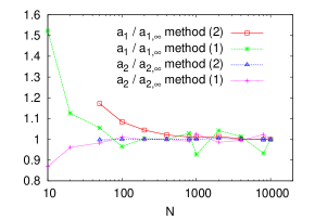
Figure 10: Parameters $a_{1}$ and $a_{2}$ in Eq. (17) plotted versus $N$. Results are obtained from two different methods mentioned in the text. Here $a_{1,\infty}$ and $a_{2,\infty}$ are taken from Table 2 for $N=10000$.

Table 2: Parameters $a_{1}$ and $a_{2}$ of the probability distribution $P(R_{g}/\ell_{b})$, Eq. (17), determined by two different methods (1) and (2) mentioned in the text for various values of chain length $N$.

$N$	10	20	50	100	200	400	800	1000	2000	4000	8000	10000
(1) $a_{1}\times 10^{4}$	7.12	5.27	4.94	4.52	4.70	4.70	4.82	4.34	4.88	4.74	4.37	4.68
(1) $a_{2}$	12.80	14.15	14.46	14.90	14.70	14.73	14.58	15.10	14.42	14.66	15.07	14.73
(2) $a_{1}\times 10^{4}$	_	_	4.14	3.83	3.69	3.60	3.57	3.56	3.58	3.54	3.53	3.53
(2) $a_{2}$	_	_	13.25	13.27	13.29	13.29	13.30	13.29	13.35	13.29	13.29	13.28

IV Semiflexible chains

We extend our simulations in this section from flexible chains to semiflexible chains. Extensive Monte Carlo simulations of semiflexible polymer chains described by standard SAWs on the simple cubic lattice, with a bending potential $U_{b}=\varepsilon_{b}(1-\cos\theta)$, have been recently carried out Hsu2010b ; Hsu2010 ; Hsu2011 . Recall that atomistic models of real chains may exhibit considerable chain stiffness due to the combined action of torsional and bond angle potentials. When a mapping to a coarse-grained model is performed, this stiffness is lumped into an effective bond angle potential of the coarse-grained model. In this standard model the angle between two subsequent bond vectors along the chain is either $0^{o}$ or $\pm 90^{o}$, and hence in the statistical weight of a SAW configuration on the lattice every $90^{o}$ bend will contribute a Boltzmann factor $q_{b}=\exp(-\varepsilon_{b}/k_{B}T)$ ($q_{b}=1$ for ordinary SAWs). $k_{B}T$ is of order unity throughout the whole paper. The partition function of such a standard SAW with $N$ bonds ($N+1$ effective monomers) and $N_{\rm bend}$ bends is therefore,

$$Z_{N}(q_{b})=\sum_{\rm config.}C_{N}(N_{\rm bend})q_{b}^{N_{\rm bend}}\,,$$ (22)

where $C_{N}(N_{\rm bend})$ is the total number of all configurations of a polymer chain of length $N$ containing $N_{\rm bend}$ bends.

We are also interested in understanding the microscopic difference between the standard SAWs and the BFM as the stiffness of chains is taken into account. Since there are $87$ bond angles possibly occurring in the chain conformations, the partition function cannot be simplified for the BFM, written as,

$$Z_{N}^{\rm(BFM)}(\varepsilon_{b})$$ (23)

$$= \sum_{\rm config.}C_{N}(\{\theta\})\exp\left[-\frac{\varepsilon_{b}}{k_{B}T}\sum_{i=1}^{N-1}(1-\cos\theta_{i,i+1})\right]\,,$$

where $\theta_{i,i+1}$ is the bond angle between the $i^{\rm th}$ bond vector and the $(i+1)^{\rm th}$ bond vector along a chain, and $C_{N}(\{\theta\})$ is the number of configurations having the same set $\{\theta\}$ but fluctuating bond lengths. In the absence of excluded volume effect, the formulas of the partition function, Eq. (22) and Eq. (23), remain the same while semiflexible chains are described by RWs and NRRWs.

IV.1 Theoretical predictions

There exist several theoretical models describing the behavior of semiflexible chains in the absence of excluded volume effects. We first consider a discrete worm-like chain model Winkler1994 that a chain consisting of $N$ bonds with fixed bond length $\ell_{b}$, but successive bonds are correlated with respect to their relative orientations,

$$\langle\vec{b}_{i}\cdot\vec{b}_{i+1}\rangle=\ell_{b}^{2}\langle\cos\theta\rangle\quad{\rm and}\quad\langle\vec{b}_{i}^{2}\rangle=\ell_{b}^{2}\,,$$ (24)

where $\theta$ is the angle between the successive bond vectors. The mean square end-to-end distance is therefore,

$$\langle R_{e}^{2}\rangle=N\ell_{b}^{2}\left[\frac{1+\langle\cos\theta\rangle}{1-\langle\cos\theta\rangle}-\frac{2\langle\cos\theta\rangle(1-(\langle\cos\theta\rangle)^{N}}{N(1-\langle\cos\theta\rangle)^{2}}\right]\,.$$ (25)

This formula agrees with the prediction for a freely rotating chain (FRC). In the limit $N\rightarrow\infty$ the bond-bond orientational correlation function decays exponentially as a function of their chemical distance $s$,

$$\langle\vec{b}_{i}\cdot\vec{b}_{i+s}\rangle=\ell_{b}^{2}\langle\cos\theta(s)\rangle=\ell_{b}^{2}\langle\cos\theta\rangle^{s}=\ell_{b}^{2}\exp(-s\ell_{b}/\ell_{p})\,,$$ (26)

where $\ell_{p}$ is the so-called persistence length which can be extracted from the initial decay of $\langle\cos\theta(s)\rangle$. Equivalently, one can calculate the persistence length from

$$\ell_{p,\theta}/\ell_{b}=-1/\ln(\langle\cos\theta\rangle)$$ (27)

here instead of $\ell_{p}$ we use $\ell_{p,\theta}$ to distinguish between these two measurements.

For rather stiff ($L\gg\ell_{p}$) and long chains ($N\rightarrow\infty$) we expect that the bond angles $\theta$ between successive bonds along chains are very small ($\langle\cos\theta\rangle\approx 1-\langle\theta^{2}\rangle/2$), then Eqs. (25) and (27) become

$$\langle R_{e}^{2}\rangle=N\ell_{b}^{2}\frac{1+\langle\cos\theta\rangle}{1-\langle\cos\theta\rangle}\approx N\ell_{b}^{2}\frac{4}{\langle\theta^{2}\rangle}\,$$ (28)

and

$$\ell_{p}/\ell_{b}=2/\langle\theta^{2}\rangle$$ (29)

Eq. (28) is equivalent to the mean square end-to-end distance of a freely jointed chain that $n_{k}$ Kuhn segments of length $\ell_{K}$ are jointed together,

$$\langle R_{e}^{2}\rangle=n_{k}\ell_{k}^{2}=2\ell_{p}L\,.$$ (30)

$L=N\ell_{b}=n_{k}\ell_{k}$ being the contour length and $\ell_{K}=2\ell_{p}$ in this limit.

In the continuum limit $\ell_{b}\rightarrow 0$, $N\rightarrow 0$, but keeping $L$ and $\ell_{p}$ finite, we obtain from Eq. (25) the prediction for a continuous worm-like chain,

$$\langle R_{e}^{2}\rangle=2\ell_{p}L\left\{1-\frac{\ell_{p}}{L}[1-\exp(-L/\ell_{p})]\right\}\,.$$ (31)

It gives the same result as that derived directly from the Kratky-Porod model Kratky1949 ; Saito1967 for worm-like chains in $d=3$,

$${\cal H}=\frac{\ell_{p}k_{B}T}{2}\int_{0}^{L}\left(\frac{\partial^{2}\vec{r}(s)}{\partial s^{2}}\right)^{2}ds\,,$$ (32)

where the polymer chain is described by the contour $\vec{r}(s)$ in continuous space. Equation (31) describes the crossover behavior from a rigid-rod for $L<\ell_{p}$, where $\langle R_{e}^{2}\rangle=L^{2}$, to a Gaussian coil for $L\gg\ell_{p}$, where $\langle R_{e}^{2}\rangle=2\ell_{p}L$ as shown in Eq. (30).

For semiflexible Gaussian chains the contour length $L=N\ell_{b}$ can also be written as $L=n_{p}\ell_{p}$ and the mean square end-to-end distance and gyration radius described in terms of $n_{p}$ and $\ell_{p}$ are Kratky1949 ; Benoit1953

$$\frac{\langle R_{e}^{2}\rangle}{2\ell_{p}L}=1-\frac{1}{n_{p}}[1-\exp(-n_{p})]\,,$$ (33)

$$\frac{6\langle R_{g}^{2}\rangle}{2\ell_{p}L}=1-\frac{3}{n_{p}}+\frac{6}{n_{p}^{2}}-\frac{6}{n_{p}^{3}}[1-\exp(-n_{p})]\,.$$ (34)

One can clearly recognize that Gaussian behavior of the radii is only seen, if the number $n_{p}$ of the persistence length that fits to a given contour length is large, $n_{p}\gg 1$, while a crossover to rigid-rod behavior occurs for $n_{p}$ of order unity.

In recent works in Ref. Wittmer2007 ; Hsu2010 ; Hsu2010b , authors have shown that the exponential decay of the bond-bond orientational correlation function, Eq. (26), and the Gaussian coil behavior, Eq. (31) for $L\gg\ell_{p}$, predicted by the worm-like chain model only hold for $s$ and $N$ up to some values $s^{*}$ and $N^{*}$, respectively when excluded volume effects are considered. The predictions of a theory based on the Flory-type free energy minimization arguments deGennes1979 ; Grosberg1994 ; Schaefer1980 ; Netz2003 proposed as an alternative to semiflexible chains with excluded volume interactions have been verified. In this treatment one considers a model where rods of length $\ell_{k}$ and diameter $D$ are jointed together, such that the contour length $L=N\ell_{b}=n_{k}\ell_{k}$. Apart from prefactors of order unity, the second virial coefficient in $d=3$ then can be estimated as

$$v_{2}=\ell_{k}^{2}D\,.$$ (35)

The free energy of a chain now contains two terms, the elastic energy taken as that of a free Gaussian, i.e., $F_{el}\approx R_{e}^{2}/(\ell_{k}L)$, and the repulsive energy due to interactions treated in mean field approximation, i.e. proportional to the square of the density $n/R^{3}$ and the volume $R^{3}$. Hence,

$$\Delta F/k_{B}T\approx R_{e}^{2}/(\ell_{K}L)+v_{2}R_{e}^{3}[(L/\ell_{K})/R_{e}^{3}]^{2}$$ (36)

Minimizing $\Delta F$ with respect to $R_{e}$, we obtain for $L\rightarrow\infty$ the standard Flory result

$$R_{e}\approx(v_{1}/\ell_{k})^{1/5}L^{3/5}=(\ell_{k}D)^{1/5}(N\ell_{b})^{3/5}\,.$$ (37)

Eq. (37) holds also for finite $L$ and $N>N^{*}=\ell_{k}^{3}/(\ell_{b}D^{2})$ since the contribution of the second term in Eq. (36) is still important. For $N<N^{*}$ the first term in Eq. (36) dominates, and the chain behaves as a Gaussian coil, $R_{e}^{2}=\ell_{k}L=\ell_{k}\ell_{b}N$, while for even smaller $N$, $N<N^{\rm rod}=\ell_{k}/\ell_{b}$, the chain behaves as a rigid-rod. Thus, the double crossover behavior of the mean square end-to-end distance is summarized as follows,

$$\langle R_{e}^{2}\rangle\approx L^{2}\,,\quad N<N^{\rm rod}=\ell_{k}/\ell_{b}\quad{\rm(rod-like\,chain)}\,,$$ (38)

$$\langle R_{e}^{2}\rangle\approx\ell_{k}L\,,\quad N^{\rm rod}<N<N^{*}\quad{\rm(Gaussian\,coil)}\,,$$ (39)

$$\langle R_{e}^{2}\rangle\approx(\ell_{k}D)^{2/5}L^{6/5}\,,\quad N>N^{*}\quad{\rm(SAW)}$$ (40)

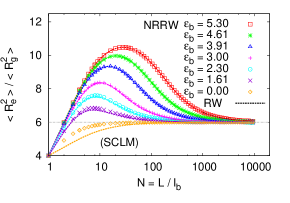
(a)      (b)

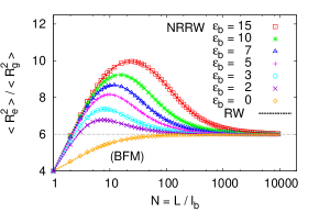
Figure 11: Ratio between mean square end-to-end distance and mean square gyration radius, $\langle R_{e}^{2}\rangle/\langle R_{g}^{2}\rangle$, plotted against chain lengths (segments) $N=L/\ell_{b}$ for SCLM (a) and for BFM (b). Data for semiflexible chains described by NRRWs and RWs are shown by symbols and lines, respectively. Here $\ell_{b}=1$ for SCLM, and $\ell_{b}=2.72$ for BFM.

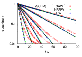
(a)      (b)

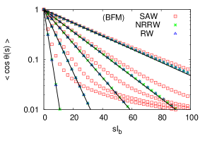
Figure 12: Semi-log plot of the bond-bond orientational correlation function $\langle\cos\theta(s)\rangle$ vs. $s\ell_{b}$ for SCLM with $\ell_{b}=1$ (a) and for BFM with $\ell_{b}=2.72$ (b). Data are for semiflexible chains described by SAWs, NRRWs and RWs and for $\varepsilon_{b}=5.30$, $4.61$, $3.91$, $3.51$, $3.00$, $2.30$ from top to bottom in (a), and for $\varepsilon_{b}=10$, $7$, $5$, $3$, and $1$ from top to bottom in (b). The straight lines indicate fits of the initial decay, $\langle\cos\theta(s)\rangle\propto\exp(-s\ell_{b}/\ell_{p})$ [Eq. (26)], for RWs.

IV.2 Simulation Results

In order to investigate the scaling behavior of the ratio $\langle R_{e}^{2}\rangle/\langle R_{g}^{2}\rangle$ for semiflexible RWs and NRRWs we plot our data $\langle R_{e}^{2}\rangle/\langle R_{g}^{2}\rangle$ versus $N=L/\ell_{b}$ for several choices of the stiffness parameter (Fig. 11). As $N$ increases, the data increase towards a maximum and then decrease towards a plateau where the prediction $\lim_{N\rightarrow\infty}\langle R_{e}^{2}\rangle/\langle R_{g}^{2}\rangle\approx 6$ for ideal chains holds. At the location of the maximum of $\langle R_{e}^{2}\rangle/\langle R_{g}^{2}\rangle$, $N=N_{h}$, the corresponding maximum values is $h={\rm max}\;\langle R_{e}^{2}\rangle/\langle R_{g}^{2}\rangle$. The maximum move monotonously to larger values as chains become stiffer. The deviation between the data for RWs and NRRWs based on the SCLM decreases as the bending energy $\varepsilon_{b}$ increases (Fig. 11a), while it is negligible for the simulation data obtained based on the BFM (Fig. 11b) in all cases.

Figure 12 shows the bond-bond orientational correlation function $\langle\cos\theta(s)\rangle$ plotted versus the chemical distance $s\ell_{b}$ covering the range from flexible chains to stiff chains characterized by $\varepsilon_{b}$ for the models SCLM and BFM. We compare the data obtained for SAWs, NRRWs, and RWs for various values of $\varepsilon_{b}$. The intrinsic stiffness remains the same for SAWs, NRRWs, and RWs as $\varepsilon_{b}$ is fixed. Results obtained from both models verify that the asymptotic exponential decay of $\langle\cos\theta(s)\rangle$ is valid only if the excluded volume effect is neglected, i.e., for RWs and NRRWs. For semiflexible SAWs $\langle\cos\theta(s)\rangle\sim\exp(-s\ell_{b}/\ell_{p})$ cannot be correct for $N\rightarrow\infty$ Wittmer2007 ; Hsu2010b , we rather have

$$\langle\vec{b}_{i}\cdot\vec{b}_{i+s}\rangle\approx s^{-\beta}\,,\enspace\beta=2-2\nu\approx 0.824\,,\enspace s^{*}\ll s\ll N\,.$$ (41)

As we have seen in Fig. 12, the exponential decay is ill-defined for rather flexible SAWs. Using Eq. (27) as a definition of the persistence length we can still give the estimate of the persistence length $\ell_{p,\theta}=-\ell_{b}/\ln\left[\langle\cos\theta(s=1)\rangle\right]$ which is approximately the same as the estimate of the decay length $\ell_{p}$ for moderately stiff chains and stiff chains. The estimates of $\ell_{p}/\ell_{b}$ and $\ell_{p,\theta}/\ell_{b}$ depending on $\varepsilon_{b}$ using Eqs. (26) and (27) are listed in Table 3 and  4. RWs are more flexible than NRRWs, and NRRWs are more flexible than SAWs from the estimates of the persistence lengths $\ell_{p}/\ell_{b}$ and $\ell_{p,\theta}/\ell_{b}$ based on the SCLM. Using the BFM the persistence lengths are almost the same in all cases of $\varepsilon_{b}$ for RWs and NRRWs, and they are smaller compared with the estimates for SAWs. Note that in Fig. 12b data deviate slightly from the fitting straight lines describing the initial exponential decay for RWs and NRRWs as the bending energy $\varepsilon_{b}$ increases, i.e., the stiffness of chains increases. For $\varepsilon_{b}>10$ the problem is more severe. Therefore, one should be careful using the BFM for studying rather stiff chains. An alternative way to the determination of the persistence length would be given by the best fit of the mean square end-to-end distance $\langle R_{e}^{2}\rangle$ of RWs or NRRWs to Eq. (31). A simple exponential decay is always found for the probability distribution of connected straight segments for semiflexible chains based on the SCLM Hsu2010 , while large fluctuations are observed for semiflexible chains based on the BFM due to bond vector fluctuations and lattice artifacts Wittmer1992 . This is the main reason why the different scenarios of the bond-bond orientational correlation functions between the SCLM and the BFM for stiff chains are seen in Fig. 12. Figure 13 shows the locations $N_{h}$ and the heights $h$ of the maximum of $\langle R_{e}^{2}\rangle/\langle R_{g}^{2}\rangle$ (Fig. 11) plotted versus the persistence length $\ell_{p}/\ell_{b}$ for semiflexible RWs based on the SCLM and BFM. Note that $N_{h}$, $h$, and $\ell_{p}/\ell_{b}$ all depend on $\varepsilon_{b}$ which controls the stiffness of chains. We see that the dependence between $h$ and $\ell_{p}/\ell_{b}$ are the same for both models, while $N_{h}$ for the BFM is slightly larger than that for the SCLM for a fixed value of $\ell_{p}/\ell_{b}$ since chains based on the BFM are more flexible.

Table 3: Two estimates for the persistence length $\ell_{p}/\ell_{b}$ from Eq. (26) and $\ell_{p,\theta}/\ell_{b}$ from Eq. (27) for semiflexible RWs, NRRWs, and SAWs with various values of $q_{b}(=\exp(-\varepsilon_{b}/k_{B}T))$ based on the SCLM ($\ell_{b}=1$). Here in our simulations values of $q_{b}$ are chosen for convenience.

	$q_{b}$	1.0	0.4	0.2	0.1	0.05	0.03	0.02	0.01	0.005
	${\varepsilon_{b}}$	0.0	0.91	1.61	2.30	3.00	3.51	3.91	4.61	5.30
$\ell_{p}/\ell_{b}$	RW	$\ldots$	0.84	1.54	2.83	5.37	8.73	12.95	25.67	51.38
	NRRW	$\ldots$	1.05	1.70	2.97	5.50	8.87	13.09	25.80	51.53
	SAW	$\ldots$	$\ldots$	2.04	3.35	5.96	9.54	13.93	26.87	52.61
$\ell_{p,\theta}/\ell_{b}$	RW	$\ldots$	0.84	1.54	2.83	5.36	8.73	12.95	25.66	51.37
	NRRW	0.62	1.05	1.70	2.98	5.50	8.87	13.08	25.79	51.53
	SAW	0.67	1.12	1.81	3.12	5.70	9.10	13.35	26.28	51.52

Table 4: Two estimates for the persistence length $\ell_{p}/\ell_{b}$ from Eq. (26) and $\ell_{p,\theta}/\ell_{b}$ from Eq. (27) for semiflexible RWs, NRRWs, and SAWs with various values of $\varepsilon_{b}$ based on the BFM ($\ell_{b}=2.72$).

	${\varepsilon_{b}}$	0.0	1.0	2.0	3.0	5.0	7.0	10.0	15
$\ell_{p}/\ell_{b}$	RW	$\ldots$	0.87	1.62	2.54	4.69	7.18	12.09	27.65
	NRRW	$\ldots$	0.87	1.62	2.54	4.69	7.18	12.09	27.65
	SAW	$\ldots$	$\ldots$	1.91	2.78	4.94	7.39	12.37	27.93
$\ell_{p,\theta}/\ell_{b}$	RW	$\ldots$	0.87	1.62	2.54	4.63	6.87	10.50	17.73
	NRRW	0.21	0.87	1.62	2.54	4.63	6.87	10.50	17.73
	SAW	0.61	1.11	1.80	2.65	4.68	6.90	10.52	17.75

The scaling plots for testing the applicability of the worm-like chain prediction, Eq. (31) and Eq. (34) to our data of $\langle R_{e}^{2}\rangle$ and $\langle R_{g}^{2}\rangle$ are shown in Fig. 14. The persistence length $\ell_{p}/\ell_{b}$ in Eq. (31) for various values of $\varepsilon_{b}$ are extracted from the exponential fit of Eq. (26) for NRRWs (see Tables 3 and 4). Since the worm-like chain model is formulated in the continuum, care has to be taken to correctly take into account the lattice structure of the present model, particularly in the rod limit. Assuming that a rigid rod consisting of $N$ monomers is located at $x_{1}=\ell_{b}$, $x_{2}=2\ell_{b}$, $\ldots$, $x_{N}=N$ along the x-axis on the simple cubic lattice, the mean square gyration radius is:

$$\langle R_{e}^{2}\rangle_{\rm rod} = \frac{1}{N}\sum_{k=1}^{N}(k\ell_{b})^{2}-\left(\frac{1}{N}\sum_{k=1}^{N}k\ell_{b}\right)^{2}$$ (42)

$$= \frac{(N+1)(2N+1)\ell_{b}^{2}}{6}-\frac{(N+1)^{2}\ell_{b}^{2}}{4}$$

$$= \frac{(N+1)(N-1)\ell_{b}^{2}}{12}=\frac{L(L+2\ell_{b})}{12}\,.$$

Therefore, due to the lattice structure, the mean square gyration radius is rescaled by $(L+2\ell_{b})$ instead of $L$ in order to compare with the theoretical predictions in Fig. 14c,d. For semiflexible RWs and NRRWs the data are indeed very well described by the worm-like chain model. As $N$ increases, we observe the crossover behavior from a rigid-rod regime to a Gaussian coil regime. The plateau value in the Gaussian regime corresponds to the persistence length $\ell_{p}/\ell_{b}$ in Fig. 14a,b and $(1/6)\ell_{p}/\ell_{b}$ in Fig. 14c,d. For SAWs the deviation from the prediction becomes more prominent as chains are more flexible since the excluded volume effects are more important.

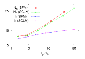
Figure 13: Location $N_{h}$ and height $h$ of the maximum of $\langle R_{e}^{2}\rangle/\langle R_{g}^{2}\rangle$ (see Fig. 11) plotted versus the persistence length $\ell_{p}/\ell_{b}$ for RWs based on the SCLM and BFM.

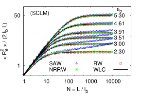
(a)     (b)

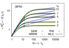
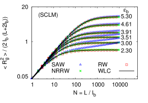
(c)     (d)

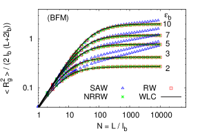
Figure 14: Log-log plots of rescaled mean square end-to-end distance $\langle R_{e}^{2}\rangle/(2\ell_{b}L)$ (a),(b) and rescaled mean square gyration radius $\langle R_{g}^{2}\rangle/(2\ell_{b}(L+2\ell_{b}))$ (c),(d) versus ${N=L/\ell_{b}}$ for semiflexible chains described by SAWs, NRRWs and RWs based on the SCLM with $\ell_{b}=1$ (a),(c) and BFM with $\ell_{b}=2.72$ (b),(d). Data for various values of $\varepsilon_{b}$ are shown, as indicated. Solid curves refer to the theoretical prediction, Eq. (31), for WLC. The values of the persistence length $\ell_{p}/\ell_{b}$ for NRRW are taken from Tables 3 and 4.

Note that one should not consider the correction factor $(L+2\ell_{b})/L$ relative to the Kratky-Porod model in Eq. (42) as a “lattice artefact”: in a real stiff polymer (e.g. an alkane-type chain) one also has a sequence of discrete individual monomers (separated by almost rigid covalent bonds along the backbone of the chain) lined up linearly (like in a rigid rod-like molecule) over about the distance of a persistence length. Furthermore, we compare simulation results of the ratio $\langle R_{e}^{2}\rangle/\langle R_{g}^{2}\rangle$ multiplied by $[(L+2\ell_{b})/L]$ as a function of ${n_{p}=L/\ell_{p}}$ to the theoretical prediction, the ratio between Eq. (33) and Eq. (34), in Fig. 15. We see the nice data collapse for RWs and NRRWs in the Gaussian regime ($n_{p}\gg 1$) and the increase of deviations from the master curve as the stiffness of chains decreases in Fig. 15a,b. The ratio $[(L+2\ell_{b})/L]\langle R_{e}^{2}\rangle/\langle R_{g}^{2}\rangle\approx 12$ as ${n_{p}\rightarrow 0}$ for a rigid-rod, while ${[(L+2\ell_{b})/L]\langle R_{e}^{2}\rangle/\langle R_{g}^{2}\rangle\approx 6}$ as $n_{p}\rightarrow\infty$ for a Gaussian coil. For SAWs we still see the nice data collapse in Fig. 15c,d, but in both rigid-rod and Gaussian coil regimes the deviations from the master curve become more prominent as chains are more flexible. For ${n_{p}>1}$ the deviation is due to the excluded volume effects, and finally $[(L+2\ell_{b})/L]\langle R_{e}^{2}\rangle/\langle R_{g}^{2}\rangle\approx 6.25$ as $n_{p}\rightarrow\infty$ for SAWs. Note that in both models the ratio of the mean square end-to-end and gyration radii exceed its asymptotic value still significantly even if $n_{p}$ is as large as ${n_{p}=10}$.

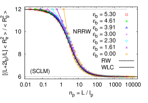
(a)     (b)

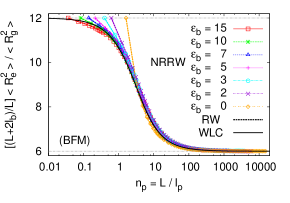
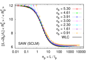
(c)     (d)

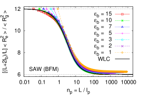
Figure 15: Semi-log plots of $[(L+2\ell_{b})/L]\langle R_{e}^{2}\rangle/\langle R_{g}^{2}\rangle$ versus $n_{p}=L/\ell_{p}$ for semiflexible chains described by RWs and NRRWs (a),(b) and SAWs (c),(d). Data for various values of $\varepsilon_{b}$ are shown, as indicated. Solid curves refer to the theoretical prediction, the ratio between Eq. (33) and Eq. (34), for WLC. The values of the persistence length $\ell_{p}/\ell_{b}$ for RWs, NRRWs, and SAWs are taken from Tables 3 and 4, respectively.

Recently, Huang et al. Huang2014a ; Huang2014b performed Brownian dynamics simulations on two-dimensional (2D) semiflexible chains described by a BSM including the excluded volume interactions. Varying the chain stiffness and chain length their results confirmed the absence of a Gaussian regime in agreement with the results from semiflexible SAWs based on the SCLM Hsu2011 , and with observations from experiments of circular single stranded DNA adsorbed on a modified graphite surface Rechendorff2099. The rescaled mean square end-to-end distance, $\langle R_{e}^{2}\rangle/(2L\ell_{p})$, in terms of $L/\ell_{p}$ for both models on the lattice and in the continuum turns out to be universal from the rigid-rod regime up to the crossover regime ($L/\ell_{p}\sim 1$) irrespective of the models chosen for the simulations. In the 2D SAW regime, different amplitude factors result from the different models Huang2014c .

In $d=3$, we indeed see the nice data collapse for semiflexible RWs, NRRWs, and SAWs in the plot of $\langle R_{e}^{2}\rangle/(2L\ell_{p})$ versus $L/2\ell_{p}$ (cf. Fig. 14a,b) from rod-like regime crossover to the Gaussian regime for $N<N^{*}$ (not shown), and the data obtained from the two lattice models are well described by the Kratky-Porod scaling function, Eq. (31). For the BSM in the continuum we should expect the same universal behavior. Although for semiflexible SAWs the second crossover from the Gaussian regime to the SAW regime for $N>N^{*}$ is rather gradual and not sharp, the relationship Hsu2012 between the crossover chain length $N^{*}$ and the persistence length $\ell_{p}/\ell_{b}$, $N^{*}\propto(\ell_{p}/\ell_{b})^{2.5}$, holds for these two models here. It would be interesting to check whether such a scaling law would also hold for the BSM.

The structure factor $S(q)$ is an experimentally accessible quantity measured by neutron scattering. We therefore also estimate $S(q)$ by

$$S(q)=\frac{1}{(N+1)^{2}}\left\langle\sum_{i=0}^{N}\sum_{j=0}^{N}\exp(i\vec{q}\cdot[\vec{r}_{i}-\vec{r}_{j}])\right\rangle$$ (43)

where $\{\vec{r}_{i}\}$ denote the positions of the $(N+1)$ monomers in a chain, and the structure factor is normalized such that $S(q\rightarrow 0)=1$. In order to compare the results of $S(q)$ obtained for fully flexible RWs, NRRWs, and SAWs based on the SCLM and BFM, we plot $S(q)$ versus $q\ell_{b}$ ($\ell_{b}=1$ for SCLM, and $\ell_{b}=2.72$ for BFM) in Fig. 16a. We see that $S(q)\approx 1-q^{2}\langle R_{g}^{2}\rangle/3$ for $q\rightarrow 0$, while for $q\gg\sqrt{\langle R_{g}^{2}\rangle}$ the power law $S(q)\sim q^{-1/\nu}$ ($\nu=0.588$ for SAWs, and $\nu=0.5$ for RWs and NRRWs) holds. The lattice artifact sets in at $q\ell_{b}\approx\pi$. Due to the local packing the first peak appears at $q\ell_{b}\approx 2\pi$ for the SCLM, while at $q\ell_{b}\approx 2.4\pi$ for the BFM as $q$ increases. In Fig. 16b we show the results for semiflexible SAWs of different stiffnesses based on the BFM. The Gaussian regime where $S(q)\sim q^{-2}$ for large values of $\varepsilon_{b}$ and then crosses gradually over to $S(q)\sim q^{-1}$ as expected for rigid rods. Neugebauer1943 .

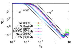
(a)     (b)

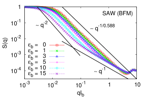
(c)

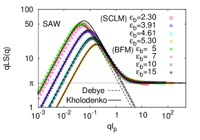
Figure 16: (a)(b) Log-log plot of structure factor $S(q)$ versus $q\ell_{b}$. Data are for fully flexible chains based on the SCLM and BFM in (a), and for semiflexible chains based on the BFM including $6$ choices of the stiffness in (b). (c) Rescaled structure factor $qLS(q)$ plotted versus $ql_{p}$. Data are for semiflexible chains based on the SCLM and BFM including $4$ choices of the stiffness each. In (a)(b), the straight lines indicate the rod-like behavior at large $q$ (slope $=-1$) the SAW behavior for flexible chains (slope $=-1/\nu$, with $\nu=0.588$), and the Gaussian behavior (slope $=-2$). In (c), the formulas proposed by Kholodenko {Eqs. (45)-(49)}, the Debye function {Eq. (44)} for Gaussian chains, and $qLS(q)\rightarrow\pi$ for a rigid-rod Neugebauer1943 are also shown for comparison.

Finally we analyze the structure factor $S(q)$ in the form of Kratky-plots, $qLS(q)$ plotted versus $q\ell_{p}$, shown in Fig. 16c for semiflexible SAWs. Data are only for $q<\pi$. The well-known theoretical predictions of the scattering from rigid-rods Neugebauer1943 , $qLS(q)\rightarrow\pi$, and Gaussian chains, the Debye function deGennes1979 ; Cloizeaux1990 ; Schaefer1999 ; Higgins1994 ,

$$S_{\rm Debye}(q)=\frac{2}{q^{2}\langle R_{g}^{2}\rangle}\left\{1-\frac{1}{q^{2}\langle R_{g}^{2}\rangle}[1-\exp(-q^{2}\langle R_{g}^{2}\rangle)]\right\}\,,$$ (44)

and the interpolation formula which describes the two limiting cases of Gaussian coils and rigid rods exactly by Kholodenko Kholodenko1993 ,

$$S(q)=\frac{2}{x}[I_{1}(x)-\frac{1}{x}I_{2}(x)],\quad x=3L/2\ell_{p}$$ (45)

where $I_{n}(x)=\int\limits_{0}^{x}dzz^{n-1}f(z)$, and the function $f(z)$ is given by

$$f(z)=\left\{\begin{array}[]{r@{\, , \quad}l}\frac{1}{E}\frac{\sinh(Ez)}{\sinh z}&q\leq\frac{3}{2\ell_{p}}\,,\\ \frac{1}{\hat{E}}\frac{\sin(\hat{E}z)}{\sinh z}&q>\frac{3}{2\ell_{p}}\,,\end{array}\right.$$ (48)

with

$$E=\left[1-\left(\frac{2q\ell_{p}}{3}\right)^{2}\right]^{1/2}\,,\quad\hat{E}=\left[\left(\frac{2q\ell_{p}}{3}\right)^{2}-1\right]^{1/2}\;,$$ (49)

are also shown for comparison Hsu2012b . Near the peak the discrepancy of our data from the theoretically predicted formulas increases as the bending energy $\varepsilon_{b}$ decreases showing that the excluded volume effect sets in. For semiflexible polymer chains of almost the same persistence length based on the two different lattice models, the structure factors are on top of each other.

V Conclusions

In this paper we have studied single polymer chains covering the range from fully flexible chains to stiff chains under very good solvent conditions by extensive Monte Carlo simulations based on two coarse-grained lattice models: the standard simple cubic lattice model and the bond fluctuation model. With the pruned-enriched Rosenbluth method the conformations of polymer chains mimicked by random walks, non-reversal random walks, and self-avoiding walks depending on the effective interactions between monomers have been analyzed in detail. We give the precise estimate of the fugacity $\mu_{\infty}$ and the entropic exponent $\gamma$ for self-avoiding walks based on the bond fluctuation model. The universal scaling predictions of mean square end-to-end distance, $\langle R_{e}^{2}\rangle$ [Eq. (2)], and mean square gyration radius, $\langle R_{g}^{2}\rangle$ [Eq. (3)], for fully flexible chains are verified as one should expect, and the corresponding amplitudes $A_{e}$ and $A_{g}$ depending on the models are determined. We have also checked the probability distributions of $R_{e}$ and $R_{g}$, $P(R_{e})$ and $P(R_{g})$, respectively. Especially we point out that the previous estimate of the parameter $A$ in Eqs. (19) for SAWs is an overestimate due to the finite-size effect. Our results also agree with the results based on the BSM Vettorel2010 , that the formula Eq. (17) predicted by Lhuillier Lhuillier1988 is a good approximate formula for RWs.

For semiflexible chains the additional regime of rod-like behavior causes slow transients in many quantities, before the asymptotic behavior of flexible chains is reached (see e.g. Fig. 11). In the absence of the excluded volume effect, a single crossover occurs, from rigid-rods to Gaussian coils as implied by the Kratky-Porod model, while a double crossover occurs from rigid-rods to Gaussian coils and then to swelling coils due to the excluded volume interaction as predicted by the Flory-like arguments. We have verified the Kratky-Porod crossover scaling behavior for semiflexible RWs, semiflexible NRRWs, and for semiflexible SAWs when the excluded volume effect is not yet important, otherwise the Flory prediction takes over for semiflexible SAWs. The flexibility of chains in our model is controlled by the bending potential ${U_{b}=\varepsilon_{b}(1-\cos\theta)}$. Our results of bond-bond orientational correlation functions ${\langle\cos\theta(s)\rangle}$ (Fig. 12) show that the persistence lengths of semiflexible RWs, NRRWs, and SAWs are the same for a given bending energy $\varepsilon_{b}$ based on the same lattice model. But, with a caveat: there is a problem of fitting the exponential decay to the data of ${\langle\cos\theta(s)\rangle}$ for not only semiflexible SAWs but also semiflexible RWs and NRRWs based on the BFM for ${\varepsilon_{b}>10}$ (rather stiff chains) due to the fluctuations of bonds and the lattice artifacts as it was mentioned in Ref. Wittmer1992 . The structure factor describing the scattering from semiflexible linear polymer chain based on the SCLM provides an almost perfect match to the result based on the BFM when we adjust the bending energy $\varepsilon_{b}$ such that the same persistence length $\ell_{p}$ results for both models.

From our simulations the different crossovers to the asymptotic behavior of single chains based on the SCLM and BFM are observed and investigated. Similar effects have to be expected for real chemical systems as well. Thus coarse graining will require different mapping ratios for different coarse-grained models. However, the equilibration time may rise dramatically for simulating large and complex realistic polymer systems. A proper mapping onto a coarse-grained model where the number of degrees of freedom is reduced should help to speed up the simulations. Based on the BFM, the bond angles and bond lengths of polymers can be treated as dynamic degrees of freedom depending on temperature. Thus, the static structure of a polymer model on the coarse grained level could be tuned, when one introduces bond length and bond angle potentials, to mimic the structure of a chemically realistic model of a polymer which contains covalent chemical bonds, whose orientation is controlled by both bond angle and torsional potentials. In this paper we did not discuss the details of this mapping procedure yet, but we hope that our work will be a useful input for this problem. However, it will also be interesting and important to understand the distributions of bond lengths and torsional angles.

We hope that the present work will contribute to a better understanding of using the lattice models for studying complex polymer systems and for the development of a multi-scale coarse-graining approach based on the lattice models.

VI Acknowledgments

I am indebted to K. Binder and K. Kremer for stimulating discussions. I thank the Max Planck Institute for Polymer Research for the hospitality while this research was carried out. I also thank the ZDV Data Center at Johannes Gutenberg University of Mainz for the use of the Mogon-Clusters and the Rechenzentrum Garching (RZG), the supercomputer center of the Max Planck Society, for the use of their computers.

References

- (1) P. J. Flory, Statistical mechanics of chain molecules, (Wiley, New York, 1969).
- (2) P. G. de Gennes, Scaling Concepts in polymer physics, (Cornell Univ. Press, Ithaca, N. Y., 1979).
- (3) K. Binder (ed.), Monte Carlo and molecular dynamics simulations in polymer science, (Oxford Univ. Press, New York, 1995).
- (4) K. Binder and W. Paul, Macromolecules 41, 4337 (2008).
- (5) M. Murat and K. Kremer, J. Chem. Phys. 108, 4340 (1998).
- (6) F. Müller-Plathe, ChemPhysChem 3, 754 (2002).
- (7) V. A. Harmandaris, N. P. Adhikari, N. F. A. van der Vegt, and K. Kremer, Macromolecules 39, 6708 (2006).
- (8) V. A. Harmandaris, D. Reith, N. F. A. van der Vegt, and K. Kremer, Macromol. Chem. Phys. 208, 2109 (2007).
- (9) P. D. Gujrati and A. L. Leonov (ed.), Modeling and simulations in polymers, (Wiley, 2010).
- (10) T. Vettorel, G. Besold, and K. Kremer, Soft Matter 6, 2282 (2010).
- (11) G. Zhang, K. Ch. Daoulas, and K. Kremer, Macromol. Chem. Phys. 214, 214 (2013).
- (12) I. Carmesin and K. Kremer, Macromolecules 21, 2819 (1988).
- (13) H. P. Deutsch and K. Binder, J. Chem. Phys. 94 2294 (1991).
- (14) W. Paul, K. Binder, D. W. Heermann, and K. Kremer, J. Phys. II 1 37 (1991).
- (15) M. Müller, in Handbook of Materials Modelingi, part B, pp2599, S. Yip (ed.), (Springer, Dordrecht, 2005).
- (16) V. Tries, W. Paul, J. Baschnagel, and K. Binder, J. Chem. Phys. 106, 738 (1997).
- (17) H.-P. Hsu, W. Paul, S. Rathgeber, and K. Binder, Macromolecules 43, 1592 (2010).
- (18) K. Lau and K. Dill, Macromolecules 11, 3986 (1989).
- (19) T. Vettorel, S. Y. Reigh, D. Y. Yoon, and K. Kremer, Macromol. Rapid Commun. 30, 345 (2009).
- (20) T. Vettorel, A. Y. Grosberg, and K. Kremer, Phys. Biol. 6, 025013 (2009).
- (21) J. D. Halverson, J. Smrek, K. Kremer, and A. Y. Grosberg, Rep. Prog. Phys. 77 022601 (2014).
- (22) J. P. Wittmer, P. Becknich, H. Mayer, A. Cavallo, A. Johner, and J. Baschnagel, J. Phys. Rev E 76, 011803 (2007).
- (23) J. D. Halverson, K. Kremer and A. Y. Grosberg, J. Phys. A: Math. Theor. 46, 065002 (2013).
- (24) S. Bhattacharya, H.-P. Hsu, A. Milchev, V. G. Rostiashvilli, and T. A. Vilgis, Macromolecules 41, 2920 (2008).
- (25) A. Huang, H.-P. Hsu, A. Bhattacharya, and K. Binder, unpublished.
- (26) S. A. Egorov, H.-P. Hsu, A. Milchev, and K. Binder, unpublished.
- (27) H.-P. Hsu and P. Grassberger, Macromolecules 37 4658 (2004).
- (28) P. Grassberger, J. Phys. A: Math. Gen. 38, 323 (2005).
- (29) B. Li, N. Madras, and A. D. Sokal, J. Stat. Phys. 80, 661 (1995).
- (30) B. G. Nickel, Macromolecules 24, 1358 (1991).
- (31) V. Privman, P. C. Hohenberg, and A. Aharony, in Phase Transitions and Critical Phenomena, VoL 14, C. Domb and J.L. Lebowitz, eds., (Academic Press, San Diego, 1991).
- (32) N. Clisby, Phys. Rev. Lett. 104, 055702 (2010).
- (33) P. Grassberger, P. Sutter, L. Schäfer, J. Phys. A 30, 7039 (1997).
- (34) K. Kremer and K. Binder, Comp. Phys. Rep. 7, 259 (1988).
- (35) P. Grassberger, Phys. Rev. E 56 3682 (1997).
- (36) H.-P. Hsu, and P. Grassberger, J. Stat. Phys. 144, 597 (2011).
- (37) D. Lhuillier, J. Phys. France 49, 705 (1988).
- (38) J. des Cloizeaux, J. Phys. France 36, 281 (1975).
- (39) M. E. Fisher, J. Chem. Phys. 44, 616 (1966).
- (40) J. M. Victor and D. Lhuillier, J. Chem. Phys. 92, 1362 (1990).
- (41) M. Bishop and C. J. Saltiel, J. Chem. Phys. 95, 606 (1991).
- (42) H.-P. Hsu, W. Paul, and K. Binder, Macromolecules 43, 3094 (2010).
- (43) H.-P. Hsu, W. Paul, and K. Binder, EPL 92 28003 (2010).
- (44) H.-P. Hsu, W. Paul, and K. Binder, EPL 95, 68004 (2011).
- (45) R. G. Winkler, P. Reineker, and L. Harnau, J. Chem. Phys 101, 8119 (1994).
- (46) O. Kratky and G. Porod, J. Colloid Sci. 4, 35 (1949)
- (47) N. Saito, K. Takahashi and Y. Yunoki, J. Phys. Soc. Jpn. 22, 219 (1967).
- (48) H. Benoit and P. Doty, J. Phys. Chem. 57, 958 (1953).
- (49) A. Yu. Grosberg and A. R. Khokhlov, Statistical Physics of Macromolecules, (AIP Press, NY, 1994).
- (50) D. W. Schaefer, J. F. Joanny, and P. Pincus, Macromolecules 13, 1280 (1980).
- (51) R. R. Netz and D. Andelman, Phys. Rep. 380, 1 (2003).
- (52) J. P. Wittmer, W. Paul, K. Binder, Macromolecules 25, 7211 (1992).
- (53) A. Huang, A. Bhattacharya, and K. Binder, J. Chem. Phys. 140, 214902 (2014).
- (54) A. Huang, R. Adhikari, A. Bhattacharya, and K. Binder, EPL 105, 18002 (2014).
- (55) K. Rechendorff, G. Witz, J. Adamcik, and G. Dietler, J. Chem. Phys. 131, 095103 (2009).
- (56) H.-P. Hsu, and K. Binder, J. Chem. Phys. 136, 024901 (2012).
- (57) T. neugebauer, Ann. Phys. 434, 509 (1943).
- (58) J. Des Cloizeaux and G. Jannink, Polymers in Solution: Their Modeling and Structure (Clarendon, Oxford, 1990).
- (59) L. Schäfer, Excluded Volume Effects in Polymer Solutions as Explained by the Renormalization Group (Springer, Berlin, 1999).
- (60) J. S. Higgins and H. C. Benoit, Polymers and Neutron Scattering (Clarendon, Oxford, 1994).
- (61) A. L. Kholodenko, Macromolecules 26, 4179 (1993).
- (62) H.-P. Hsu, and W. Paul, and K. Binder, J. Chem. Phys. 137, 174902 (2012).