On some non-linear projections of self-similar sets in $\mathbb{R}^{3}$

Abstract.

In the last years considerable attention has been paid for the orthogonal projections and non-linear images of self-similar sets. In this paper we consider homothetic self-similar sets in $\mathbb{R}^{3}$, i.e. the generating IFS has the form $\left\{\lambda_{i}\underline{x}+\underline{t}_{i}\right\}_{i=1}^{q}$. We show that if the dimension of the set is strictly bigger than $1$ then the image of the set under some non-linear functions onto the real line has dimension $1$. As an application, we show that the distance set of such self-similar sets has dimension $1$. Moreover, the third algebraic product of a self-similar set with itself on the real line has dimension $1$ if its dimension is at least $1/3$.

1. Introduction and Statements

We call a non-empty compact set $\Lambda$ self-similar in $\mathbb{R}^{d}$ if there exists an iterated function system (IFS) $\Phi$ of the form

$$\Phi=\left\{f_{i}(\underline{x})=\lambda_{i}O_{i}\underline{x}+\underline{t}_{i}\right\}_{i=1}^{q},$$ (1.1)

where $\lambda_{i}\in(0,1)$, $\underline{t}_{i}\in\mathbb{R}^{d}$ and $O_{i}$ is an orthogonal transformation of $\mathbb{R}^{d}$ for every $i=1,\dots,q$, and $\Lambda$ is the attractor of $\Phi$, i.e. the unique non-empty compact set $\Lambda=\bigcup_{i=1}^{q}f_{i}(\Lambda)$. We call a measure $\mu$ self-similar if there exists an IFS $\Phi$ in the form (1.1) and a probability vector $(p_{1},\dots,p_{q})$ such that $\mu=\sum_{i=1}^{q}p_{i}(f_{i})_{*}\mu$, where $(f)_{*}\mu=\mu\circ f^{-1}$.

Let us denote the set of orthogonal projections from $\mathbb{R}^{d}$ to $\mathbb{R}^{k}$ by $\Pi_{d,k}$. The classical results of Marstrand [15] and Kaufman [14] states that for any $A\subseteq\mathbb{R}^{d}$ Borel set $\dim_{H}\pi A=\min\left\{k,\dim_{H}A\right\}$ for almost every $\pi\in\Pi_{d,k}$, where $\dim_{H}$ denotes the Hausdorff dimension. Let us denote the packing dimension by $\dim_{P}$ and the box dimension by $\dim_{B}$. For the definition and basic properties of Hausdorff, packing and box dimension we refer to [3].

Hochman and Shmerkin [13] proved that if the IFS $\Phi$ satisfies the strong separation condition (SSC), i.e. $f_{i}(\Lambda)\cap f_{j}(\Lambda)=\emptyset$ for every $i\neq j$ and the orthogonal transformations of the IFS $\Phi$ satisfies a minimality assumption, that is there exists a $\pi\in\Pi_{d,k}$ such that

$$\bigcup_{n=1}^{\infty}\left\{\pi O_{i_{1}}\cdots O_{i_{n}}:1\leq i_{1},\dots,i_{n}\leq q\right\}$$ (1.2)

is dense in $\Pi_{d,k}$, then $\dim_{H}\pi\Lambda=\min\left\{k,\dim_{H}\Lambda\right\}$ for every $\pi\in\Pi_{d,k}$, moreover, $\dim_{H}g(\Lambda)=\min\left\{k,\dim_{H}\Lambda\right\}$ for every $g\in C^{1}(\mathbb{R}^{d}\mapsto\mathbb{R}^{k})$ without singular points. In particular, if the minimality assumption holds then (1.2) holds for all $\pi\in\Pi_{d,k}$. Recently, Farkas [7] generalized this result by omitting the strong separation condition.

Dekking [2], Rams and Simon [19, 20], Falconer and Jin [5] considered the orthogonal projections and non-linear images of random self-similar sets. For more detailed surveys on projections of fractal sets and measures, see [4] or [21].

In this paper, we focus on homothetic self-similar sets (HSS set) in $\mathbb{R}^{3}$, which is $O_{i}=I$ for every $i=1,\cdots,q$, where $I$ denotes the identity. Similarly, we consider homothetic self-similar measures (HSS measure).

It is well known fact that in this case the dimension may drop under some orthogonal projections. However, if $\Lambda$ is a HSS set with SSC on $\mathbb{R}^{2}$ then $\dim_{H}g(\Lambda)=\min\left\{1,\dim_{H}\Lambda\right\}$ for certain $g:\mathbb{R}^{2}\mapsto\mathbb{R}$ $C^{2}$ functions. This result was first published in the paper of Bond, Łaba and Zahl [1, Proposition 2.6], but they attribute the proof to Hochman.

Our goal is to generalize this result for HSS sets in $\mathbb{R}^{3}$, at least in the case when $\dim_{H}\Lambda$ is large enough.

During the paper we will have a special interest on the radial projection $P_{d}:\mathbb{R}^{d}\setminus\{\underline{0}\}\mapsto S^{d-1}$, where $S^{d-1}$ denotes the unit sphere in $\mathbb{R}^{d}$. Precisely, $P_{d}(\underline{x})=\frac{\underline{x}}{\|\underline{x}\|}$. For simplicity, denote the gradient vector of a function $g:\mathbb{R}^{d}\mapsto\mathbb{R}$ at a point $\underline{x}$ by $\nabla_{\underline{x}}g$.

Theorem 1.1.

Let $\Lambda$ be an homothetic self-similar set in $\mathbb{R}^{3}$ such that $\dim_{H}\Lambda>1$ and $\Lambda$ is not contained in any plane (but not necessarily satisfying SSC). Suppose that $g:\mathbb{R}^{3}\mapsto\mathbb{R}$ is a $C^{1}$ function on a $V\supseteq\Lambda$ open set such that

1. $\|\nabla_{\underline{x}}g\|\neq 0$ for every $\underline{x}\in\Lambda$,

2. $\|\nabla_{t\cdot\underline{x}}g\times\nabla_{\underline{x}}g\|=0$ for every $\underline{x}\in V$ and for every $t\in\mathbb{R}$ such that $t\cdot\underline{x}\in V$.

3. The function $h_{g}$ is bi-Lipschitz on $P_{3}(\Lambda)\subseteq S^{2}$, where $h_{g}(\underline{x})=P_{3}(\nabla_{t\cdot\underline{x}}g)$ for any $t\in\mathbb{R}$ such that $t\cdot\underline{x}\in V$.

Then $\dim_{H}g(\Lambda)=1$.

We apply Theorem 1.1 in two ways. First, we show a corollary for the distance set of HSS sets in $\mathbb{R}^{3}$. Let us denote the distance set of $A\subset\mathbb{R}^{d}$ by $D(A)$. That is,

$$D(A)=\left\{\|\underline{x}-\underline{y}\|:\underline{x},\underline{y}\in A\right\}.$$ (1.3)

For every $\underline{x}\in A$, we define the pinned distance set of $A\subset\mathbb{R}^{d}$ at the point $\underline{x}$ by

$$D_{\underline{x}}(A)=\left\{\|\underline{x}-\underline{y}\|:\underline{y}\in A\right\}.$$ (1.4)

Falconer’s distance set conjecture states that if $\dim_{H}A>d/2$ then $D(A)$ has positive Lebesgue measure for any measurable $A\subseteq\mathbb{R}^{d}$. Recently, Orponen [17] showed that for any self-similar set $\Lambda$ in $\mathbb{R}^{2}$ if $\mathcal{H}^{1}(\Lambda)>0$ then $\dim_{H}D(\Lambda)=1$, where $\mathcal{H}^{1}$ denotes the Hausdorff measure. We improve Orponen’s result for HSS sets in $\mathbb{R}^{3}$ in the following way.

Theorem 1.2.

Let $\Lambda$ be an HSS set in $\mathbb{R}^{3}$ such that $\dim_{H}\Lambda>1$. Then for every $\underline{x}\in\Lambda$, $\dim_{H}D_{\underline{x}}(\Lambda)=1$. In particular, $\dim_{H}D(\Lambda)=1$.

As a second application, we consider the algebraic product of a self-similar set on the real line with itself. Let $A,B\subset\mathbb{R}$ and denote $A\cdot B$ the algebraic product $A$ and $B$, that is,

$$A\cdot B=\left\{x\cdot y:x\in A\text{ and }y\in B\right\}.$$

As a consequence of the result of Bond, Łaba and Zahl [1] we show that for every $\Lambda$ self-similar set on the real line

$$\dim_{H}\Lambda\cdot\Lambda=\min\left\{2\dim_{H}\Lambda,1\right\},$$ (1.5)

see Corollary 2.9. We generalize this result for $\Lambda\cdot\Lambda\cdot\Lambda$ in the following way.

Theorem 1.3.

Let $\Lambda$ be a self-similar set in $\mathbb{R}$ such that $\dim_{H}\Lambda>1/3$. Then $\dim_{H}\Lambda\cdot\Lambda\cdot\Lambda=1$.

2. Preliminaries and non-linear projections in $\mathbb{R}^{2}$

This section is devoted to enumerate our tools to prove Theorem 1.1. The results on the projections in $\mathbb{R}^{2}$ were previously studied by several authors, e.g. Hochman [10], Hochman and Shemrkin [13], Bond, Łaba and Zahl [1] etc. For the convenience of the reader, we state here these theorems and give short proofs.

First, we introduce some notations. Let $\Phi$ be an IFS on $\mathbb{R}^{d}$ with contracting similitudes in the form (1.1). Denote the attractor of $\Phi$ by $\Lambda$. Let us denote the set of symbols by $\mathcal{S}=\left\{1,\dots,q\right\}$ and the symbolic space by $\Sigma=\mathcal{S}^{\mathbb{N}}$. Denote $\sigma$ the left-shift operator on $\Sigma$. Let us define the natural projection $\rho$ from $\Sigma$ to $\Lambda$ in the usual way, i.e. for any $\mathbf{i}=(i_{0},i_{1},\dots)\in\Sigma$

$$\rho(\mathbf{i})=\lim_{n\rightarrow\infty}f_{i_{0}}\circ f_{i_{1}}\circ\cdots\circ f_{i_{n}}(\underline{0}),$$

where $\underline{0}=(0,\dots,0)\in\mathbb{R}^{d}$. It is easy to see that $\rho(\mathbf{i})=f_{i_{0}}(\rho(\sigma\mathbf{i}))$.

Let $\underline{p}=(p_{1},\dots,p_{q})$ be a probability vector with strictly positive elements. Denote the Bernoulli measure on $\Sigma$ by $\nu=\underline{p}^{\mathbb{N}}$, then $\nu$ is left-shift invariant and ergodic. Then the measure $\mu=\rho_{*}\nu=\nu\circ\rho^{-1}$ is the unique self-similar measure with $\mathrm{spt}\mu=\Lambda$ and $\mu=\sum_{i=1}^{q}p_{i}(f_{i})_{*}\mu$.

Let us denote the finite length words of symbols $\mathcal{S}$ by $\Sigma^{*}=\bigcup_{n=0}^{\infty}\mathcal{S}^{n}$. For an $\overline{\imath}=(i_{0},\dots,i_{n-1})\in\Sigma^{*}$, denote $|\overline{\imath}|$ the length of $\overline{\imath}$ and for any $\overline{\imath},\overline{\jmath}\in\Sigma^{*}$, denote the juxtaposition $\overline{\imath}\overline{\jmath}$ the finite length word $(i_{0},\dots,i_{|\overline{\imath}|-1},j_{0},\dots,j_{|\overline{\jmath}|-1})$.

For the composition of functions $f_{i_{0}}\circ\cdots\circ f_{i_{n-1}}$, we write $f_{\overline{\imath}}$, where $\overline{\imath}=(i_{0},\dots,i_{n-1})$. We denote the fixed point of a function $f_{\overline{\imath}}$ by $\mathrm{Fix}(f_{\overline{\imath}})$. Denote $[\overline{\imath}]$ the cylinder set formed by $\overline{\imath}$,

$$[\overline{\imath}]:=\left\{\mathbf{j}=(j_{0},j_{1},\dots)\in\Sigma:i_{0}=j_{0},\dots,i_{|\overline{\imath}|-1}=j_{|\overline{\imath}|-1}\right\}.$$

We denote the projection of a cylinder set by $\Lambda_{\overline{\imath}}=\rho([\overline{\imath}])=f_{\overline{\imath}}(\Lambda)$, and we call it as a cylinder set of $\Lambda$. We note that if $\mu$ is a HSS measure (or $\Lambda$ is a HSS set) with IFS $\Phi=\left\{f_{i}(\underline{x})=\lambda_{i}\underline{x}+\underline{t}_{i}\right\}_{i=1}^{q}$ in $\mathbb{R}^{d}$ with SSC then for any $\overline{\imath}\in\Sigma^{*}$ the measure $\mu_{\overline{\imath}}:=\frac{\left.\mu\right|_{\Lambda_{\overline{\imath}}}}{\mu(\Lambda_{\overline{\imath}})}$ (or respectively $\Lambda_{\overline{\imath}}$) is also a self-similar measure (or self-similar set) with IFS $\Phi_{\overline{\imath}}:=\left\{\lambda_{i}\underline{x}+f_{\overline{\imath}}(t_{i})\right\}_{i=1}^{q}$. On the other hand, for any $\pi\in\Pi_{d,k}$ the measure $\pi\mu=\mu\circ\pi^{-1}$ is HSS measure (or respectively $\pi\Lambda$ is a HSS set), as well, with IFS $\pi\Phi:=\left\{\lambda x+\pi(\underline{t}_{i})\right\}_{i=1}^{q}$. We denote the $n$th iteration of the IFS by $\Phi^{n}=\left\{f_{\overline{\imath}}\right\}_{\overline{\imath}\in\mathcal{S}^{n}}$.

Our first approach of the study of homothetic self-similar sets is to find proper approximating subsystem.

Proposition 2.1.

Let $\Lambda$ be an HSS set in $\mathbb{R}^{d}$ with IFS $\Phi=\left\{f_{i}(\underline{x})=\lambda_{i}\underline{x}+\underline{t}_{i}\right\}_{i=1}^{q}$. For every $\varepsilon>0$, there exists an IFS $\Phi^{\prime}$ of the form $\left\{g_{j}(\underline{x})=\lambda\underline{x}+\underline{t}_{j}^{\prime}\right\}_{j=1}^{q^{\prime}}$ with $\lambda\in(0,1)$ such that the attractor $\Lambda^{\prime}$ of $\Phi^{\prime}$ satisfies the SSC, $\Lambda^{\prime}\subseteq\Lambda$ and $\dim_{H}\Lambda^{\prime}>\dim_{H}\Lambda-\varepsilon$. Moreover, the functions of $\Phi^{\prime}$ can be written as the composition of functions in $\Phi$.

We call the attractor and self-similar measures of such a system $\Phi^{\prime}$ as homogeneous homothetic self-similar set and measures (HHSS).

The proof is analogous to the proof of Peres and Shmerkin [18, Proposition 6], therefore we omit it.

Let us denote the Hausdorff dimension of a measure $\mu$ by $\dim_{H}\mu$. That is,

$$\dim_{H}\mu=\inf\left\{\dim_{H}A:\mu(A)>0\right\}.$$

Let us define the upper and lower local dimension of a measure $\mu$ at a point $\underline{x}$ in the usual way by

$$\underline{d}_{\mu}(\underline{x})=\liminf_{r\rightarrow 0+}\frac{\log\mu(B_{r}(\underline{x}))}{\log r}\text{ and }\overline{d}_{\mu}(\underline{x})=\limsup_{r\rightarrow 0+}\frac{\log\mu(B_{r}(\underline{x}))}{\log r},$$

where $B_{r}(\underline{x})$ is the ball with radius $r$ centered at $\underline{x}$. By [6, Theorem 1.2],

$$\dim_{H}\mu=\mu-\mathrm{essinf}_{\underline{x}}\underline{d}_{\mu}(\underline{x}).$$ (2.1)

We say that the measure $\mu$ is exact dimensional if $\underline{d}_{\mu}(\underline{x})=\overline{d}_{\mu}(\underline{x})$ for $\mu$-a.e. $\underline{x}$. By [6, Corollary 2.1], if $\mu$ is exact dimensional then

$$\dim_{H}\mu=\inf\left\{\dim_{H}A:\mu(A)=1\right\}.$$

Lemma 2.2.

Let $\mu$ and $\nu$ be Borel probability measures such that $\mu\ll\nu$ (that is, $\mu$ is absolutely continuous with respect to $\nu$) and $\nu$ is exact dimensional. Then $\dim_{H}\mu=\dim_{H}\nu$.

Proof.

Since $\mu\ll\nu$, for any measurable set $A$, if $\mu(A)>0$ then $\nu(A)>0$. Thus, $\dim_{H}\mu\geq\dim_{H}\nu$. On the other hand, since $\nu$ is exact dimensional

$$\dim_{H}\nu=\inf\left\{\dim_{H}A:\nu(A)=1\right\}=\inf\left\{\dim_{H}A:\nu(A^{c})=0\right\}\geq\\ \inf\left\{\dim_{H}A:\mu(A^{c})=0\right\}=\inf\left\{\dim_{H}A:\mu(A)=1\right\}\geq\dim_{H}\mu,$$

where $A^{c}$ denotes the complement of $A$. ∎

Our second approach is to approximate the non-linear projections of HSS measures with SSC by orthogonal projections. Let $g:\mathbb{R}^{d}\mapsto\mathbb{R}$ be a $C^{1}$ function. We denote the projection of a Borel measure $\mu$ on $\mathbb{R}^{d}$ by $g_{*}\mu=\mu\circ g^{-1}$. Let us denote the gradient of $g$ at a point $\underline{x}=(x_{1},\dots,x_{d})$ by $\nabla_{\underline{x}}g$, i.e.

$$\nabla_{\underline{x}}g=\left(\begin{array}[]{c}g^{\prime}_{x_{1}}(\underline{x})\\ \vdots\\ g^{\prime}_{x_{d}}(\underline{x})\end{array}\right).$$

Denote $\pi_{g,\underline{x}}\in\Pi_{d,1}$ the orthogonal projection from $\mathbb{R}^{d}$ to the subspace spanned by $\nabla_{\underline{x}}g$, that is, $\pi_{g,\underline{x}}(\underline{y})\leavevmode\nobreak\ =\leavevmode\nobreak\ \frac{<\nabla_{\underline{x}}g,\underline{y}>}{\|\nabla_{\underline{x}}g\|}$, where $<.,.>$ denotes the standard scalar product on $\mathbb{R}^{d}$ and $\|.\|$ denotes the induced norm. The next theorem is a consequence of the results of Hochman [10].

Theorem 2.3.

Let $\mu$ be an HSS measure with SSC in $\mathbb{R}^{d}$ and let $g:\mathbb{R}^{d}\mapsto\mathbb{R}$ be a $C^{1}$ function with $\|\nabla_{\underline{x}}g\|\neq 0$ for every $\underline{x}\in\mathrm{spt}\mu$. Then

$$\dim_{H}g_{*}\mu\geq\mu-\mathrm{essinf}_{\underline{x}}\dim_{H}\pi_{g,\underline{x}}\mu.$$

Proof.

Let $\mu$ be an HSS measure with SSC in $\mathbb{R}^{d}$. Then by [10, Example 4.3] the measure $\mu$ is a homogeneous uniformly scaling measure, see [10, Definition 1.5(3) and Defintion 1.35]. Let $P$ be the ergodic fractal distribution generated by $\mu$, see [10, Definition 1.2, Definition 1.5(1) and Proposition 1.36]. For a $\pi\in\Pi_{d,1}$, let

$$E_{P}(\pi)=\int\dim_{H}\pi\nu dP(\nu).$$

Applying [10, Theorem 1.23] and [10, Proposition 1.36] we have for any $g:\mathbb{R}^{d}\mapsto\mathbb{R}$ $C^{1}$ function with $\|\nabla_{\underline{x}}g\|\neq 0$

$$\dim_{H}g_{*}\mu\geq\mu-\mathrm{essinf}_{\underline{x}}E_{P}(\pi_{g,\underline{x}}).$$

By [10, Proposition 1.36] for $P$-a.e $\nu$ measure there exists a ball $B$ that $\mu\ll(T_{B})_{*}\nu$, where $T_{B_{r}(\underline{x})}(\underline{y})=\frac{\underline{y}-\underline{x}}{r}$. Hence, $\pi\mu\ll\pi(T_{B})_{*}\nu$ for every $\pi\in\Pi_{d,1}$ and $P$-a.e. $\nu$. On the other hand, by [10, Theorem 1.22] the measure $\pi\nu$ is exact dimensional for $P$-a.e. $\nu$. Since $T_{B}$ is a bi-Lipschitz map, by Lemma 2.2, $\dim_{H}\pi\mu=\dim_{H}\pi\nu$ for every $\pi\in\Pi_{d,1}$ and $P$-a.e. $\nu$, which implies that $E_{P}(\pi)=\dim_{H}\pi\mu$. ∎

As a consequence of Theorem 2.3 and [11, Theorem 1.8], we state here a modified version of the proposition of Hochman, published in Bond, Łaba and Zahl [1, Proposition 2.6].

Proposition 2.4.

Let $\mu$ be a HHSS measure with SSC in $\mathbb{R}^{2}$ such that $\mathrm{spt}\mu$ is not contained in any line. Suppose that $g:\mathbb{R}^{2}\mapsto\mathbb{R}$ $C^{2}$ map such that $\|\nabla_{\underline{x}}g\|\neq 0$ and

$$\left\|\left(\begin{array}[]{c}g_{xx}^{\prime\prime}(\underline{x})g_{y}^{\prime}(\underline{x})-g_{xy}^{\prime\prime}(\underline{x})g_{x}^{\prime}(\underline{x})\\ g_{xy}^{\prime\prime}(\underline{x})g_{y}^{\prime}(\underline{x})-g_{yy}^{\prime\prime}(\underline{x})g_{x}^{\prime}(\underline{x})\end{array}\right)\right\|\neq 0$$

for every $\underline{x}\in\mathrm{spt}\mu$. Then

$$\dim_{H}g_{*}\mu=\min\left\{1,\dim_{H}\mu\right\}.$$

Before we prove the proposition, we need a technical lemma.

Lemma 2.5.

Let $\mu$ be a HHSS measure with SSC in $\mathbb{R}^{2}$ such that $\mathrm{spt}\mu$ is not contained in any line. Then there exists a constant $c>0$ that $\dim_{H}\pi\mu\geq c>0$ for every $\pi\in\Pi_{2,1}$.

Proof.

Let $\mu$ be a HHSS measure with SSC in $\mathbb{R}^{2}$ such that $\mathrm{spt}\mu$ is not contained in any line and let $\left\{f_{i}(\underline{x})=\lambda\underline{x}+\underline{t}_{i}\right\}_{i=1}^{q}$ the corresponding IFS and $\underline{p}=(p_{1},\dots,p_{q})$ the corresponding probability vector.

Since $\mathrm{spt}\mu$ is not contained in any line, there exist three fixed points of the functions, let say $f_{1},f_{2}$ and $f_{3}$, form a triangle. Let us denote the sides of the triangle by $a$, $b$ and $c$. Let $\kappa=\inf_{\pi\in\Pi_{2,1}}\max\left\{|\pi a|,|\pi b|,|\pi c|\right\}>\leavevmode\nobreak\ 0$ and let $N=\lceil\frac{\log\kappa/(4|\mathrm{spt}\mu|)}{\log\lambda}\rceil$, where $|.|$ denotes the diameter of a set. Let $x\in\pi\mathrm{spt}\mu$ be arbitrary, and let

$$z_{n}(x):=\sum_{\begin{subarray}{c}\overline{\imath}\in\mathcal{S}^{nN}\\ B_{\frac{\kappa}{4}\lambda^{nN}}(x)\cap\pi\Lambda_{\overline{\imath}}\neq\emptyset\end{subarray}}\nu([\overline{\imath}]).$$

It is easy to see by the definition of $N$ and $\kappa$ that there exists an $\overline{\imath}\in\Sigma^{*}$ with $|\overline{\imath}|=N$ that $B_{\frac{\kappa}{4}\lambda^{N}}(x)\cap\pi\Lambda_{\overline{\imath}}=\emptyset$. Thus, $z_{1}(x)\leq(1-p_{\min}^{N})$, where $p_{\min}=\min\left\{p_{1},\dots,p_{q}\right\}$. On the other hand, for every $\overline{\imath}\in\Sigma^{*}$ with $|\overline{\imath}|=nN$ and $B_{\frac{\kappa}{4}\lambda^{nN}}(x)\cap\pi\Lambda_{\overline{\imath}}\neq\emptyset$ there exists a $\overline{\jmath}\in\Sigma$ with $|\overline{\jmath}|=N$ that $B_{\frac{\kappa}{4}\lambda^{(n+1)N}}(x)\cap\pi\Lambda_{\overline{\imath}\overline{\jmath}}=\emptyset$. Thus,

$$\sum_{\begin{subarray}{c}\overline{\jmath}\in\mathcal{S}^{N}\\ B_{\frac{\kappa}{4}\lambda^{(n+1)N}}(x)\cap\pi\Lambda_{\overline{\imath}\overline{\jmath}}\neq\emptyset\end{subarray}}\nu([\overline{\jmath}])\leq 1-p_{\min}^{N}.$$ (2.2)

Now we prove by induction that $z_{n}(x)\leq(1-p_{\min}^{N})^{n}$. For $n=1$ it has already been showed. Assume that it holds for $n$. Then by (2.2)

$$z_{n+1}(x)=\sum_{\begin{subarray}{c}\overline{\imath}\in\mathcal{S}^{(n+1)N}\\ B_{\frac{\kappa}{4}\lambda^{(n+1)N}}(x)\cap\pi\Lambda_{\overline{\imath}}\neq\emptyset\end{subarray}}\nu([\overline{\imath}])=\sum_{\begin{subarray}{c}\overline{\imath}\in\mathcal{S}^{nN}\\ B_{\frac{\kappa}{4}\lambda^{nN}}(x)\cap\pi\Lambda_{\overline{\imath}}\neq\emptyset\end{subarray}}\sum_{\begin{subarray}{c}\overline{\jmath}\in\mathcal{S}^{N}\\ B_{\frac{\kappa}{4}\lambda^{(n+1)N}}(x)\cap\pi\Lambda_{\overline{\imath}\overline{\jmath}}\neq\emptyset\end{subarray}}\nu([\overline{\imath}\overline{\jmath}])=\\ \sum_{\begin{subarray}{c}\overline{\imath}\in\mathcal{S}^{nN}\\ B_{\frac{\kappa}{4}\lambda^{nN}}(x)\cap\pi\Lambda_{\overline{\imath}}\neq\emptyset\end{subarray}}\nu([\overline{\imath}])\sum_{\begin{subarray}{c}\overline{\jmath}\in\mathcal{S}^{N}\\ B_{\frac{\kappa}{4}\lambda^{(n+1)N}}(x)\cap\pi\Lambda_{\overline{\imath}\overline{\jmath}}\neq\emptyset\end{subarray}}\nu([\overline{\jmath}])\leq(1-p_{\min}^{N})z_{n}(x)\leq(1-p_{\min}^{N})^{n+1}.$$

Hence, for any $x\in\mathrm{spt}\mu$

$$\liminf_{r\rightarrow 0+}\frac{\log\mu(B_{r}(x))}{\log r}=\liminf_{n\rightarrow\infty}\frac{\log\mu(B_{\frac{\kappa}{4}\lambda^{nN}}(x))}{nN\log\lambda}\geq\liminf_{n\rightarrow\infty}\frac{\log z_{n}(x)}{nN\log\lambda}=\frac{\log(1-p_{\min}^{N})}{N\log\lambda}>0.$$

Which implies by (2.1) that $\dim_{H}\pi\mu\geq\frac{\log(1-p_{\min}^{N})}{N\log\lambda}>0$ for every $\pi\in\Pi_{2,1}$. ∎

Proof of Proposition 2.4.

Let $\mu$ be a HHSS measure with SSC such that $\mathrm{spt}\mu$ is not contained in any line. Since $\dim_{H}g_{*}\mu\leq\min\left\{1,\dim_{H}\mu\right\}$, it is enough to show the lower bound. By Theorem 2.3 we have

$$\dim_{H}g_{*}\mu\geq\mu-\mathrm{essinf}_{\underline{x}}\dim_{H}\pi_{g,\underline{x}}\mu.$$

Thus, it is enough to show that

$$\dim_{H}\pi_{g,\underline{x}}\mu=\min\left\{1,\dim_{H}\mu\right\}\text{ for $\mu$-a.e. $\underline{x}$.}$$ (2.3)

If $\mu$ is a HHSS measure with IFS $\left\{\lambda\underline{x}+\underline{t}_{i}\right\}_{i=1}^{q}$ then for any $\pi\in\Pi_{2,1}$ the measure $\pi\mu$ is HHSS measure, as well, with IFS $\left\{\lambda x+\pi(\underline{t}_{i})\right\}_{i=1}^{q}$. By using the parametrization $\pi_{\theta}(\underline{x})=<(\cos\theta,\sin\theta),\underline{x}>$ and [11, Theorem 1.8], it follows that

$$\dim_{P}\left\{\theta\in[0,\pi):\dim_{H}\pi_{\theta}\mu<\min\left\{1,\dim_{H}\mu\right\}\right\}=0.$$

Hence, to verify (2.3) it is enough to show that

$$\dim_{H}f_{*}\mu>0,$$

where $f(\underline{x})=\arctan\left(\frac{g^{\prime}_{x_{1}}(\underline{x})}{g_{x_{2}}^{\prime}(\underline{x})}\right)$. By our assumption $\|\nabla_{\underline{x}}f\|\neq 0$ for every $\underline{x}\in\mathrm{spt}\mu$. By applying Theorem 2.3 and Lemma 2.5, we get

$$\dim_{H}f_{*}\mu\geq\mu-\mathrm{essinf}_{\underline{x}}\dim_{H}\pi_{f,\underline{x}}\mu\geq\inf_{\pi\in\Pi_{2,1}}\dim_{H}\pi\mu\geq c>0.$$

∎

As a consequence of Proposition 2.4, we state here the analogue of [1, Proposition 2.5] but for measures, which plays important role for the further studies.

Corollary 2.6.

If $\mu$ is a HHSS measure with SSC in $\mathbb{R}^{2}$ such that $\underline{0}\notin\mathrm{spt}\mu$ and $\mathrm{spt}\mu$ is not contained in any line then

$$\dim_{H}(P_{2})_{*}\mu=\min\left\{1,\dim_{H}\mu\right\}.$$ (2.4)

Proof.

Since $\mu$ can be written as a convex combination of self-similar measures restricted to cylinder sets, we have

$$\dim_{H}(P_{2})_{*}\mu=\min_{\overline{\imath}\in\mathcal{S}^{n}}\dim_{H}(P_{2})_{*}\mu_{\overline{\imath}}$$

for every $n\geq 1$. Thus it is enough to show that for sufficiently large $n\geq 1$ (2.4) holds for any $\overline{\imath}\in\mathcal{S}^{n}$. By choosing $n$ sufficiently large and by applying a rotation transformation, without loss of generality we may assume that $\mathrm{spt}\mu_{\overline{\imath}}$ is contained in the upper half plane and it is separated away from the $x$-axis.

Since the map $h:x\mapsto(x,\sqrt{1-x^{2}})$ is bi-Lipschitz for every $x\in(-1+\varepsilon,1+\varepsilon)$, it is enough to show that for the map $g:(x,y)\mapsto\frac{x}{\sqrt{x^{2}+y^{2}}}$, $\dim_{H}g_{*}\mu_{\overline{\imath}}=\min\left\{1,\dim_{H}\mu_{\overline{\imath}}\right\}.$ Indeed, $g$ satisfies the assumptions of Proposition 2.4. ∎

As another consequence of Proposition 2.4 we can state the following theorem for general self-similar sets in $\mathbb{R}^{2}$.

Theorem 2.7.

Let $\Lambda$ be an arbitrary self-similar set in $\mathbb{R}^{2}$ not contained in any line. Suppose that $g:\mathbb{R}^{2}\mapsto\mathbb{R}$ is a $C^{2}$ map such that $\|\nabla_{\underline{x}}g\|\neq 0$ and

$$\left\|\left(\begin{array}[]{c}g_{xx}^{\prime\prime}(\underline{x})g_{y}^{\prime}(\underline{x})-g_{xy}^{\prime\prime}(\underline{x})g_{x}^{\prime}(\underline{x})\\ g_{xy}^{\prime\prime}(\underline{x})g_{y}^{\prime}(\underline{x})-g_{yy}^{\prime\prime}(\underline{x})g_{x}^{\prime}(\underline{x})\end{array}\right)\right\|\neq 0$$

for every $\underline{x}\in\Lambda$. Then

$$\dim_{H}g(\Lambda)=\min\left\{1,\dim_{H}\Lambda\right\}.$$

Proof.

Let $\Lambda$ be a self-similar set in $\mathbb{R}^{2}$ not contained in any line. Applying [17, Lemma 3.4], for every $\varepsilon>0$ there exists a self-similar set $\Lambda^{\prime}\subseteq\Lambda$ not contained in any line such that $\dim_{H}\Lambda^{\prime}\geq\dim_{H}\Lambda-\varepsilon$ and its the attractor of IFS $\Phi^{\prime}$ satisfying SSC. If one of the functions of $\Phi^{\prime}$ contains an irrational rotation then by [13, Corollary 1.7]

$$\dim_{H}g(\Lambda)\geq\dim_{H}g(\Lambda^{\prime})=\min\left\{1,\dim_{H}\Lambda^{\prime}\right\}\geq\min\left\{1,\dim_{H}\Lambda\right\}-\varepsilon.$$

If none of the functions of $\Phi^{\prime}$ contains irrational rotation then by [17, Lemma 4.2] there exists a self-similar set $\Lambda^{\prime\prime}\subseteq\Lambda$ such that $\dim_{H}\Lambda^{\prime\prime}\geq\dim_{H}\Lambda-2\varepsilon$ and the similitudes of generating IFS $\Phi^{\prime\prime}$ of $\Lambda^{\prime\prime}$ do not contain any rotation or reflection, i.e. it is a HSS set with SSC. By Proposition 2.1, there exists a HHSS set $\Lambda^{\prime\prime\prime}$ with SSC that $\Lambda^{\prime\prime\prime}\subseteq\Lambda$ and $\dim_{H}\Lambda^{\prime\prime\prime}\geq\dim_{H}\Lambda-3\varepsilon$.

Let $\mu$ be the natural self-similar measure on $\Lambda^{\prime\prime\prime}$, that is, $\mu$ is the equidistributed self-similar measure on the cylinder sets. Hence, $\dim_{H}\mu=\dim_{H}\Lambda^{\prime\prime\prime}$. By Proposition 2.4,

$$\dim_{H}g(\Lambda)\geq\dim_{H}g_{*}\mu=\min\left\{1,\dim_{H}\mu\right\}=\min\left\{1,\dim_{H}\Lambda^{\prime\prime\prime}\right\}\geq\min\left\{1,\dim_{H}\Lambda\right\}-3\varepsilon.$$

Since $\varepsilon>0$ was arbitrary, the statement of the theorem is proven. ∎

As a corollary of Theorem 2.7, one can prove a weaker version of Falconer’s distance set conjecture in $\mathbb{R}^{2}$. This is just a little bit stronger than Orponen’s result [17, Theorem 1.2], since we only assume that $\dim_{H}\Lambda\geq 1$ and we do not need that $\mathcal{H}^{1}(\Lambda)>0$.

Corollary 2.8.

If $\Lambda$ is a self-similar set in $\mathbb{R}^{2}$ with $\dim_{H}\Lambda\geq 1$. Then

$$\dim_{H}D(\Lambda)=1,$$

where $D(\Lambda)$ denotes the distance set of $\Lambda$ defined in (1.3).

Proof.

If $\Lambda$ is contained in a line then $\dim_{H}D(\Lambda)=\dim_{H}\Lambda$. So, we may assume that $\Lambda$ is not contained in any line. Let $\underline{a}$ be an arbitrary element of $\Lambda$ and let $\Lambda_{\overline{\imath}}$ be a cylinder set such that $\mathrm{dist}(\underline{a},\Lambda_{\overline{\imath}})>0$. Then $D_{\underline{a}}(\underline{x})=\|\underline{x}-\underline{a}\|$ satisfies the conditions of Theorem 2.7 with self-similar set $\Lambda_{\overline{\imath}}$. Thus,

$$\dim_{H}D(\Lambda)\geq\dim_{H}D_{\underline{a}}(\Lambda)\geq\dim_{H}D_{\underline{a}}(\Lambda_{\overline{\imath}})=\min\left\{1,\dim_{H}\Lambda_{\overline{\imath}}\right\}=\min\left\{1,\dim_{H}\Lambda\right\}=1.$$

∎

Another corollary of Theorem 2.7 is (1.5).

Corollary 2.9.

If $\Lambda$ is a self-similar set in $\mathbb{R}$ then $\dim_{H}\Lambda\cdot\Lambda=\min\left\{2\dim_{H}\Lambda,1\right\}$.

Proof.

Let $\Lambda$ be an arbitrary self-similar set on $\mathbb{R}$. Without loss of generality, we may assume that $\Lambda$ is not a singleton. Then there exists a cylinder set $\Lambda_{\overline{\imath}}$ of $\Lambda$ that every element in $\Lambda_{\overline{\imath}}$ is either strictly positive or strictly negative.

By [18, Proposition 6], for every $\varepsilon>0$ there exists a self-similar set $\Lambda^{\prime}\subseteq\Lambda_{\overline{\imath}}$ such that $\dim_{H}\Lambda^{\prime}\geq\dim_{H}\Lambda-\varepsilon$ and its the attractor of IFS $\Phi$ satisfying SSC and has the form

$$\Phi=\left\{f_{i}(x)=\lambda x+t_{i}\right\}_{i=1}^{q}.$$

Then $\Lambda^{\prime}\times\Lambda^{\prime}$ is a self-similar set with SSC in $\mathbb{R}^{2}$ with IFS

$$\Phi^{\prime}=\left\{h_{i}(\underline{x})=\lambda\underline{x}+(t_{i},t_{j})\right\}_{i,j=1}^{q}.$$

Let $g(x,y)=xy$. Then

$$\|\nabla_{\underline{x}}g\|=\sqrt{y^{2}+x^{2}}\neq 0\text{ and }\left\|\left(\begin{array}[]{c}g_{xx}^{\prime\prime}(\underline{x})g_{y}^{\prime}(\underline{x})-g_{xy}^{\prime\prime}(\underline{x})g_{x}^{\prime}(\underline{x})\\ g_{xy}^{\prime\prime}(\underline{x})g_{y}^{\prime}(\underline{x})-g_{yy}^{\prime\prime}(\underline{x})g_{x}^{\prime}(\underline{x})\end{array}\right)\right\|=\sqrt{x^{2}+y^{2}}\neq 0$$

for any $(x,y)\in\mathbb{R}^{2}\backslash\left\{(0,0)\right\}$. Thus by Theorem 2.7

$$\dim_{H}\Lambda\cdot\Lambda\geq\dim_{H}\Lambda^{\prime}\cdot\Lambda^{\prime}=\dim_{H}g(\Lambda^{\prime}\times\Lambda^{\prime})=\min\left\{1,\dim_{H}\Lambda^{\prime}\times\Lambda^{\prime}\right\}\geq\min\left\{1,2\dim_{H}\Lambda\right\}-2\varepsilon,$$

where we used that $\dim_{H}\Lambda^{\prime}\times\Lambda^{\prime}=2\dim_{H}\Lambda^{\prime}$, see [3, Corollary 7.4]. Since $\varepsilon>0$ was arbitrary, the proof is complete. ∎

Similarly to the proof of Proposition 2.4, to prove our main Theorem 1.1, we need an upper bound for the exceptional directions for the orthogonal projections in $\Pi_{3,1}$. For a vector $\underline{n}\in S^{d-1}$ let $\pi_{\underline{n}}\in\Pi_{d,1}$ be the orthogonal projection to the subspace generated by $\underline{n}$, i.e. $\pi_{\underline{n}}(\underline{x})=<\underline{x},\underline{n}>$.

Proposition 2.10.

Let $\mu$ be a HHSS measure in $\mathbb{R}^{3}$ with SSC. Then

$$\dim_{P}\left\{\underline{n}\in S^{2}:\dim_{H}\pi_{\underline{n}}\mu<\min\left\{1,\dim_{H}\mu\right\}\right\}\leq 1.$$ (2.5)

Proposition 2.10 follows from Hochman [12, Theorem 1.10].

Finally, we state here the dimension conservation phenomena for HSS measures, first showed by Furstenberg [9] and generalized by Falconer and Jin [5].

Theorem 2.11.

Let $\mu$ be an HSS measure with SSC in $\mathbb{R}^{d}$ and let $\pi\in\Pi_{d,k}$ be arbitrary. Then

$$\dim_{H}\pi\mu+\dim_{H}\mu_{\pi^{-1}(\underline{x})}=\dim_{H}\mu\text{ for $\pi\mu$-a.e. $\underline{x}\in\mathbb{R}^{k}$,}$$ (2.6)

where $\mu_{\pi^{-1}(\underline{x})}$ denote the conditional measures of $\mu$ on the fibres $\pi^{-1}(\underline{x})$. Moreover,

$$\pi\mapsto\dim_{H}\pi\mu\text{ is lower semi-continuous.}$$ (2.7)

For the proof of the theorem we refer to Hochman [10, Theorem 1.37].

3. Radial projection in $\mathbb{R}^{3}$

The critical point of our study is the examination of the radial projection. Unfortunately, we cannot prove the analogue of Corollary 2.6 in general. However, we are able to show that if an HSS set has dimension strictly larger than $1$ then there exists a HHSS measure such that its support is contained in the HSS set, and its radial projection has dimension strictly larger than $1$.

Theorem 3.1.

Let $\Lambda$ be a HSS set in $\mathbb{R}^{3}$ such that $\dim_{H}\Lambda>1$ and $\Lambda$ is not contained in any plane. Then there exists a $\mu$ HHSS measure such that $\mathrm{spt}\mu\subseteq\Lambda$ and $\dim_{H}\mu\geq\dim_{H}(P_{3})_{*}\mu>1$.

Let us denote the closed double cone with vertex $\underline{x}\in\mathbb{R}^{3}$, angle $\alpha$, and axis $\underline{v}\in\mathbb{R}^{3}$ with $\|\underline{v}\|=1$ by $C_{\alpha,\underline{v}}(\underline{x})$. That is,

$$C_{\alpha,\underline{v}}(\underline{x})=\left\{\underline{y}\in\mathbb{R}^{3}:|<\underline{x}-\underline{y},\underline{v}>|\geq|\cos(\alpha)|\|\underline{x}-\underline{y}\|\right\}.$$

In other words, the angle between $\underline{x}-\underline{y}$ and $\underline{v}$ is less than or equal to $\alpha$. First, we show the following lemma.

Lemma 3.2.

Let $\Lambda$ be a HHSS set in $\mathbb{R}^{3}$ such that it is not contained in any plane. Then for every vector $\underline{v}\in\mathbb{R}^{3}$ with $\|\underline{v}\|=1$ and $\underline{x}\in\Lambda$ there exists an $\pi/2>\alpha>0$ such that for every $r>0$

$$\mathrm{int}(B_{r}(\underline{x})\cap C_{\alpha,\underline{v}}(\underline{x}))\cap\Lambda\neq\emptyset,$$

where $\mathrm{int}(A)$ denotes the interior of a set $A$.

Proof.

We argue by contradiction. Assume that there exist vector $\underline{v}\in\mathbb{R}^{3}$ with $\|\underline{v}\|=1$ and $\underline{x}\in\Lambda$ such that for every $\pi/2>\alpha>0$ there exists an $r=r(\alpha)>0$ that

$$\mathrm{int}(B_{r}(\underline{x})\cap C_{\alpha,\underline{v}}(\underline{x}))\cap\Lambda=\emptyset.$$

Let $\Phi=\left\{f_{i}(\underline{x})=\lambda\underline{x}+\underline{t}_{i}\right\}_{i=1}^{q}$ be the corresponding IFS and let $n(r)=\min\left\{n:\lambda^{n}<r\right\}$.

For a $\pi/2>\alpha>0$ if $\underline{x}\in\Lambda_{\overline{\imath}}$ with $|\overline{\imath}|\geq n(r(\alpha))$ then $\Lambda_{\overline{\imath}}\subseteq\mathrm{int}(B_{r(\alpha)}(\underline{x}))\cap\Lambda$. Thus by our assumption $\Lambda_{\overline{\imath}}\cap\mathrm{int}(C_{\alpha,\underline{v}}(\underline{x}))=\emptyset.$ Since $\Phi$ does not contain any orthogonal transformation.

$$\Lambda\cap\mathrm{int}(C_{\alpha,\underline{v}}(f_{\overline{\imath}}^{-1}(\underline{x})))=f_{\overline{\imath}}^{-1}(\Lambda_{\overline{\imath}}\cap\mathrm{int}(C_{\alpha,\underline{v}}(\underline{x})))=\emptyset.$$

Thus, for every $\pi/2>\alpha>0$ there exists a $N\geq 1$ such that for every $\overline{\imath}$ with $\underline{x}=\rho(\mathbf{i})=f_{\overline{\imath}}(\rho(\sigma^{|\overline{\imath}|}\mathbf{i}))$ and $|\overline{\imath}|\geq N$

$$\Lambda\cap\mathrm{int}(C_{\alpha,\underline{v}}(f_{\overline{\imath}}^{-1}(\underline{x})))=\emptyset.$$

Let $\underline{y}$ be a density point of the sequence $\left\{f_{\overline{\imath}}^{-1}(\underline{x})\right\}$. Since $\Lambda$ is compact, $\underline{y}\in\Lambda$ and $\Lambda\cap\mathrm{int}C_{\alpha,\underline{v}}(\underline{y})=\emptyset.$ But $\alpha$ was arbitrary, thus $\Lambda$ must be contained in a plane with normal vector $\underline{v}$ and containing $\underline{y}$ which is a contradiction. ∎

Denote by $V_{\pi}$ the subspace to which $\pi\in\Pi_{3,2}$ projects and denote the normal vector of $V_{\pi}$ by $\underline{n}_{\pi}\in\mathbb{R}^{3}$ with $\|\underline{n}_{\pi}\|=1$. For a projection $\pi\in\Pi_{3,2}$, let

$$\sin(\varepsilon_{\pi})=\inf_{\underline{x}\neq\underline{y}\in\Lambda}\frac{\|\underline{n}_{\pi}\times(\underline{x}-\underline{y})\|}{\|\underline{x}-\underline{y}\|}.$$ (3.1)

Since $\Lambda$ is compact, if $\pi\Lambda$ satisfies the SSC then $\sin(\varepsilon_{\pi})>0$ . Let $\Gamma_{\pi}$ be as follows

$$\Gamma_{\pi}=\left\{(\underline{x},\underline{y})\in\Lambda\times\Lambda:\underline{x}\neq\underline{y}\ \&\ \sin(\varepsilon_{\pi})=\frac{\|\underline{n}_{\pi}\times(\underline{x}-\underline{y})\|}{\|\underline{x}-\underline{y}\|}\right\}.$$

Since $\Phi=\{f_{i}\}_{i=1}^{q}$ is orthogonal transformation free,

$$\sin(\varepsilon_{\pi})=\min_{i\neq j}\inf_{\underline{x}\in f_{i}(\Lambda),\underline{y}\in f_{j}(\Lambda)}\frac{\|\underline{n}_{\pi}\times(\underline{x}-\underline{y})\|}{\|\underline{x}-\underline{y}\|}.$$

Moreover, by compactness, there are $i\neq j$, $\underline{x}_{i}\in f_{i}(\Lambda)$, $\underline{y}_{j}\in f_{j}(\Lambda)$ such that $(\underline{x}_{i},\underline{y}_{j})\in\Gamma_{\pi}\neq\emptyset$. By definition

$$\mathrm{int}\left(C_{\varepsilon_{\pi},\underline{n}_{\pi}}(\underline{x})\right)\cap\Lambda=\emptyset\text{ for every $\underline{x}\in\Lambda$.}$$ (3.2)

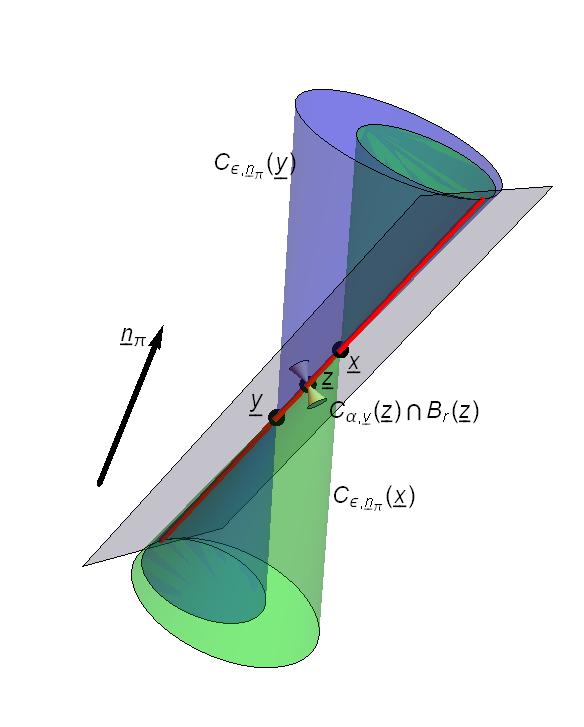
Figure 1. Cones and points for $(\underline{x},\underline{y}),(\underline{x},\underline{z}),(\underline{y},\underline{z})\in\Gamma_{\pi}$.

Lemma 3.3.

Let $\Lambda$ be a HHSS set not contained in any plane and suppose that $\pi\Lambda$ satisfies the SSC. If $(\underline{x},\underline{y}),(\underline{x},\underline{z})\in\Gamma_{\pi}$ then $(\underline{y},\underline{z})\notin\Gamma_{\pi}$. Thus, if $(\underline{x},\underline{y})\in\Gamma_{\pi}$ then $l_{\underline{x},\underline{y}}\cap\Lambda\backslash\{\underline{x},\underline{y}\}=\emptyset$, where $l_{\underline{x},\underline{y}}$ is the line containing $\underline{x}$ and $\underline{y}$.

Proof.

Let us suppose that $(\underline{x},\underline{y}),(\underline{x},\underline{z}),(\underline{y},\underline{z})\in\Gamma_{\pi}$. It is easy to see that $\underline{x},\underline{y},\underline{z}$ must be contained in one line. Indeed, $\underline{z}$ must be a common element of the boundary of the cones $C_{\varepsilon_{\pi},\underline{n}_{\pi}}(\underline{x})$ and $C_{\varepsilon_{\pi},\underline{n}_{\pi}}(\underline{y})$, see Figure 1. Without loss of generality, assume that $\underline{z}$ is between $\underline{x}$ and $\underline{y}$. Let $V$ be the common tangent plane of the cones $C_{\varepsilon_{\pi},\underline{n}_{\pi}}(\underline{x})$ and $C_{\varepsilon_{\pi},\underline{n}_{\pi}}(\underline{y})$, and let $\underline{v}$ be its normal vector. Applying Lemma 3.2, there exists an $\pi/2>\alpha>0$ that $\mathrm{int}(B_{r}(\underline{z})\cap C_{\alpha,\underline{v}}(\underline{z}))\cap\Lambda\neq\emptyset,$ for every $r>0$. Let $r>0$ be sufficiently small that $\mathrm{int}(B_{r}(\underline{z})\cap C_{\alpha,\underline{v}}(\underline{z}))\subseteq\mathrm{int}(C_{\varepsilon_{\pi},\underline{n}_{\pi}}(\underline{x})\cap C_{\varepsilon_{\pi},\underline{n}_{\pi}}(\underline{y}))$. Then

$$\emptyset\neq\mathrm{int}(B_{r}(\underline{z})\cap C_{\alpha,\underline{v}}(\underline{z}))\cap\Lambda\subseteq\mathrm{int}(C_{\varepsilon_{\pi},\underline{n}_{\pi}}(\underline{x}))\cap\Lambda.$$

But by (3.2), $\mathrm{int}(C_{\varepsilon_{\pi},\underline{n}_{\pi}}(\underline{x}))\cap\Lambda=\emptyset$, which is a contradiction. ∎

Proposition 3.4.

Let $\Lambda$ be a HSS set in $\mathbb{R}^{3}$ such that $\dim_{H}\Lambda>1$ and it is not contained in any plane. Then there exists an orthogonal projection $\pi\in\Pi_{3,2}$ and a self-similar measure $\mu$ such that $\mathrm{spt}\mu\subseteq\Lambda$, $\mathrm{spt}\mu$ is not contained in any plane, $\pi\mu$ satisfies the SSC (but not w.r.t the IFS generating $\mu$), and $\dim_{H}\mu>\dim_{H}\pi\mu>1$.

Proof.

Let $\Lambda$ be a HSS set satisfying the assumptions. By Marstrand’s projection theorem [16, Corollary 9.4, Corollary 9.8] there exists a $\pi_{1}\in\Pi_{3,2}$ such that $\dim_{H}\pi_{1}\Lambda=\min\left\{2,\dim_{H}\Lambda\right\}$. The set $\pi_{1}\Lambda$ is a HSS set in $\mathbb{R}^{2}$. Applying Proposition 2.1, there exists a HHSS set $\Lambda^{1}$ and an IFS $\Phi_{1}=\left\{f_{i}(\underline{x})=\lambda\underline{x}+\underline{t}_{i}\right\}_{i=1}^{q}$ with SSC such that $\Lambda^{1}\subseteq\Lambda$, $\pi_{1}\Lambda^{1}$ satisfies the SSC and $2>\dim_{H}\Lambda^{1}=\dim_{H}\pi_{1}\Lambda^{1}>1$.

Let $\varepsilon_{\pi_{1}}$ be defined in (3.1). By compactness, there are $\underline{x}_{i}\in f_{i}(\Lambda^{1})$, $\underline{y}_{j}\in f_{j}(\Lambda^{1})$ such that $i\neq j$ and $(\underline{x}_{i},\underline{y}_{j})\in\Gamma_{\pi_{1}}$. Let us fix such $i\neq j$ and $\underline{x}_{i},\underline{y}_{j}$. Denote the projection onto the subspace with normal vector $\frac{\underline{x}_{i}-\underline{y}_{j}}{\|\underline{x}_{i}-\underline{y}_{j}\|}$ by $\pi_{2}$. Then by Lemma 3.3, the projection $\pi_{2}$ is 2 to 1 on $\Lambda^{1}$. Thus, by [8, Corollary 4.16], $\dim_{H}\Lambda^{1}=\dim_{H}\pi_{2}\Lambda^{1}$, but clearly, the SSC does not hold.

Let $\delta>0$ be sufficiently small such that $\dim_{H}\Lambda^{1}-3\delta>1$. Let us fix $\overline{\imath},\overline{\jmath}\in\Sigma^{*}$ such that $|\overline{\imath}|=|\overline{\jmath}|$, $\underline{x}_{i}\in f_{\overline{\imath}}(\Lambda^{1})$, $\underline{y}_{j}\in f_{\overline{\jmath}}(\Lambda^{1})$ and choose $m:=|\overline{\imath}|=|\overline{\jmath}|$ sufficiently large that the attractor $\widetilde{\Lambda}$ of the IFS $\widetilde{\Phi}:=\left\{f_{i_{0}}\circ\cdots\circ f_{i_{m-1}}\right\}_{i_{0},\dots,i_{m-1}=1}^{q}\backslash\left\{f_{\overline{\imath}},f_{\overline{\jmath}}\right\}$ satisfies $\dim_{H}\widetilde{\Lambda}\geq\dim_{H}\Lambda^{1}-\delta$. Since $\pi_{2}$ is still at most 2 to 1 on the smaller set $\widetilde{\Lambda}$, we have $\dim_{H}\widetilde{\Lambda}=\dim_{H}\pi_{2}\widetilde{\Lambda}$. Let us observe that $\pi_{2}\underline{x}_{i}=\pi_{2}\underline{y}_{j}\notin\pi_{2}\widetilde{\Lambda}$.

Let $\widetilde{\mu}$ be the natural HSS measure on $\widetilde{\Lambda}$. By Theorem 2.11(2.7) the function $\pi\mapsto\dim_{H}\pi\widetilde{\mu}$ is lower semi-continuous at $\pi_{2}$. Hence, $\pi\mapsto\dim_{H}\pi\widetilde{\Lambda}$ is lower semi-continuous at $\pi_{2}$. Let $\beta>0$ sufficiently small such that for every projection $\pi\in\Pi_{3,2}$, with $\|\underline{n}_{\pi}\times\underline{n}_{\pi_{2}}\|<|\sin(\beta)|$, $\pi\underline{x}_{i},\pi\underline{y}_{j}\notin\pi\widetilde{\Lambda}$ and

$$\dim_{H}\pi\widetilde{\Lambda}\geq\dim_{H}\pi_{2}\widetilde{\Lambda}-\delta=\dim_{H}\widetilde{\Lambda}-\delta.$$

Since the fixed points of the iterates of the functions are dense in $\widetilde{\Lambda}$, by compactness, we may find $\hbar_{1},\hbar_{2}\in\Sigma^{*}$ that $\pi(\mathrm{Fix}(f_{\overline{\imath}\hbar_{1}})),\pi(\mathrm{Fix}(f_{\overline{\jmath}\hbar_{2}}))\notin\pi\widetilde{\Lambda}$ for every projection $\pi\in\Pi_{3,2}$, with $\|\underline{n}_{\pi}\times\underline{n}_{\pi_{2}}\|<|\sin(\beta)|$ and

$$\frac{\|(\mathrm{Fix}(f_{\overline{\imath}\hbar_{1}})-\mathrm{Fix}(f_{\overline{\jmath}\hbar_{2}}))\times(\underline{x}_{i}-\underline{y}_{j})\|}{\|\mathrm{Fix}(f_{\overline{\imath}\hbar_{1}})-\mathrm{Fix}(f_{\overline{\jmath}\hbar_{2}})\|\|\underline{x}_{i}-\underline{y}_{j}\|}<|\sin(\beta)|.$$

Denote the projection onto the subspace with normal vector $\frac{\mathrm{Fix}(f_{\overline{\imath}\hbar_{1}})-\mathrm{Fix}(f_{\overline{\jmath}\hbar_{2}})}{\|\mathrm{Fix}(f_{\overline{\imath}\hbar_{1}})-\mathrm{Fix}(f_{\overline{\jmath}\hbar_{2}})\|}$ by $\pi^{\prime}$. Applying Proposition 2.1 for $\pi^{\prime}\widetilde{\Phi}$, there exist a HHSS set $\widetilde{\Lambda}^{1}$ and an IFS $\widetilde{\Phi}_{1}$ with SSC such that $\widetilde{\Lambda}^{1}\subseteq\widetilde{\Lambda}$, $\pi^{\prime}\widetilde{\Lambda}^{1}$ satisfies the SSC and $\dim_{H}\widetilde{\Lambda}^{1}=\dim_{H}\pi^{\prime}\widetilde{\Lambda}^{1}>\dim_{H}\pi^{\prime}\widetilde{\Lambda}-\delta$.

We claim that there exist $m,k\geq 1$ that the IFS $\left(\pi^{\prime}\widetilde{\Phi}_{1}\right)^{m}\cup\left\{\overbrace{\pi^{\prime}f_{\overline{\imath}\hbar_{1}}\circ\cdots\circ\pi^{\prime}f_{\overline{\imath}\hbar_{1}}}^{k}=:\pi^{\prime}f_{\overline{\imath}\hbar_{1}}^{k}\right\}$ satisfies the SSC and it is homogeneous.

Indeed, since the system $\pi^{\prime}\widetilde{\Phi}_{1}$ satisfies SSC and is homogeneous, then for every $m\geq 1$ $\left(\pi^{\prime}\widetilde{\Phi}_{1}\right)^{m}$ still satisfies SSC and is homogeneous. By Proposition 2.1, the contraction ratio of $\widetilde{\Phi}_{1}$ is $\lambda^{l}$ for an $l\geq 1$. On the other hand, the contraction ratio of $f_{\overline{\imath}\hbar_{1}}$ is $\lambda^{|\overline{\imath}\hbar_{1}|}$. Now, let us fix the ratio $k/m=l/|\overline{\imath}\hbar_{1}|$. Since $\pi^{\prime}(\mathrm{Fix}(f_{\overline{\imath}\hbar_{1}})),\pi^{\prime}(\mathrm{Fix}(f_{\overline{\jmath}\hbar_{2}}))\notin\pi^{\prime}\widetilde{\Lambda}$, by choosing $k$ sufficiently large, the SSC holds.

Let $\Phi^{\prime}:=(\widetilde{\Phi}_{1})^{m}\cup\left\{f_{\overline{\imath}\hbar_{1}}^{k},f_{\overline{\imath}\hbar_{2}}^{k}\right\}$ and its attractor $\Lambda^{\prime}$. Observe that $\pi^{\prime}(\mathrm{Fix}(f_{\overline{\imath}\hbar_{1}}))=\pi^{\prime}(\mathrm{Fix}(f_{\overline{\jmath}\hbar_{2}}))$. Thus, $\pi^{\prime}f_{\overline{\imath}\hbar_{1}}\equiv\pi^{\prime}f_{\overline{\imath}\hbar_{2}}$, i.e. there are exact overlaps. Hence, $\pi^{\prime}\Phi^{\prime}=\left(\pi^{\prime}\widetilde{\Phi}_{1}\right)^{m}\cup\left\{\pi^{\prime}f_{\overline{\imath}\hbar_{1}}^{k}\right\}$ and therefore, satisfies SSC.

Let $\Lambda^{\prime}$ be the attractor of $\Phi^{\prime}$. Then

$$\dim_{H}\pi^{\prime}\Lambda^{\prime}\geq\dim_{H}\pi^{\prime}\widetilde{\Lambda}^{1}\geq\dim_{H}\pi^{\prime}\widetilde{\Lambda}-\delta\geq\dim_{H}\pi_{2}\widetilde{\Lambda}-2\delta=\dim_{H}\widetilde{\Lambda}-2\delta\geq\dim_{H}\Lambda^{1}-3\delta>1.$$

Let $\mu^{\prime}$ be the HHSS measure on $\Lambda^{\prime}$ with weights $\frac{1}{\sharp\left(\widetilde{\Phi}_{1}\right)^{m}+1}$ for the functions in $\left(\widetilde{\Phi}_{1}\right)^{m}$ and weights $\frac{1}{2(\sharp\left(\widetilde{\Phi}_{1}\right)^{m}+1)}$ for the functions $f_{\overline{\imath}\hbar_{1}}^{k},f_{\overline{\imath}\hbar_{2}}^{k}$. Thus, $\pi^{\prime}\mu^{\prime}$ is the natural self-similar measure on $\pi^{\prime}\Lambda^{\prime}$ and therefore, $1<\dim_{H}\pi^{\prime}\Lambda^{\prime}=\dim_{H}\pi^{\prime}\mu^{\prime}$. Because of the exact overlap and the fact that $\mathrm{spt}\pi^{\prime}\mu^{\prime}=\pi^{\prime}\Lambda^{\prime}$ cannot be contained in a line, $\mathrm{spt}\mu^{\prime}$ cannot be contained in a plane. The exact overlap and $\dim_{H}\mu^{\prime}\leq\dim_{H}\Lambda^{1}<2$ imply $\dim_{H}\mu^{\prime}>\dim_{H}\pi^{\prime}\mu^{\prime}$, which had to be proven. ∎

By changing the coordinates, without loss of generality we may assume that the projection in Proposition 3.4 is a coordinate projection $\pi:(x,y,z)\mapsto(x,y)$. Moreover, since the measure $\mu$ in Proposition 3.4 cannot be contained in any plane, we may assume that $\mathrm{spt}\mu$ is supported on an octant, separated away from the $z$ axis by restricting $\mu$ to a cylinder set.

Let us denote the projection along geodesics on $S^{2}$ to $S^{1}$ by $\gamma$. We note that $\gamma$ is well defined except on the poles. On the other hand, $\gamma\circ P_{3}=P_{2}\circ\pi$.

Let $\nu:=(P_{3})_{*}\mu$. Thus, $\gamma_{*}\nu=(P_{2})_{*}\pi\mu$. By convenience, we use the cylindrical coordinates in $\mathbb{R}^{3}$ and the radial coordinates on $\mathbb{R}^{2}$. That is, for $\mathbb{R}^{3}\ni\underline{x}=(r,\varphi,z)$, $\pi(\underline{x})=(r,\varphi)$, $P_{2}(\pi(\underline{x}))=\varphi=\gamma(P_{3}(\underline{x}))$. Let us denote the conditional measures of $\mu$ on $\pi^{-1}(r,\varphi)$ by $\mu_{\pi^{-1}(r,\varphi)}$, the conditional measures of $\pi\mu$ on $P_{2}^{-1}(\varphi)$ by $\pi\mu_{P_{2}^{-1}(\varphi)}$, and the conditional measures of $\nu$ on $\gamma^{-1}(\varphi)$ by $\nu_{\gamma^{-1}(\varphi)}$, see Figure 2.

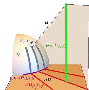
Figure 2. The conditional and projected measures along $P_{2},P_{3}$ and $\gamma$.

Lemma 3.5.

For $\gamma_{*}\nu$-almost every $\varphi\in S^{1}$, $\dim_{H}\nu_{\gamma^{-1}(\varphi)}\geq\dim_{H}\mu-\dim_{H}\pi\mu>0$.

Proof.

By definition of conditional measures $\nu=\int\nu_{\gamma^{-1}(\varphi)}d\gamma_{*}\nu(\varphi)$. On the other hand, $\pi\mu=\int\pi\mu_{P_{2}^{-1}(\varphi)}d\gamma_{*}\nu(\varphi)$ and thus, $\mu=\int\mu_{\pi^{-1}(r,\varphi)}d\pi\mu(r,\varphi)=\iint\mu_{\pi^{-1}(r,\varphi)}d\pi\mu_{P_{2}^{-1}(\varphi)}(r)d\gamma_{*}\nu(\varphi)$. Hence,

$$\nu=(P_{3})_{*}\mu=\iint(P_{3})_{*}\mu_{\pi^{-1}(r,\varphi)}d\pi\mu_{P_{2}^{-1}(\varphi)}(r)d\gamma_{*}\nu(\varphi).$$

Since the conditional measures are uniquely defined up to a zero measure set

$$\nu_{\gamma^{-1}(\varphi)}=\int(P_{3})_{*}\mu_{\pi^{-1}(r,\varphi)}d\pi\mu_{P_{2}^{-1}(\varphi)}(r)\text{ for $\gamma_{*}\nu$-almost every $\varphi$.}$$ (3.3)

Let us observe that for any compact line segment $I\subset\mathbb{R}^{3}$ which is not contained in any $1$ dimensional subspace of $\mathbb{R}^{3}$ the map $P_{3}:I\mapsto S^{2}$ is bi-Lipschitz. Hence, by Theorem 2.11(2.6) and Proposition 3.4

$$\dim_{H}(P_{3})_{*}\mu_{\pi^{-1}(r,\varphi)}=\dim_{H}\mu_{\pi^{-1}(r,\varphi)}=\dim_{H}\mu-\dim_{H}\pi\mu>0\text{ for $\pi\mu$-a.e. $(r,\varphi)$.}$$

By using the definition of Hausdorff dimension, let $A_{\varphi,n}$ be the set such that $\nu_{\gamma^{-1}(\varphi)}(A_{\varphi,n})>0$ and$\dim_{H}\nu_{\gamma^{-1}(\varphi)}\geq\dim_{H}A_{\varphi,n}-\frac{1}{n}$. Thus, by (3.3) for $\gamma_{*}\nu$-a.e. $\varphi$ there exists a set $B_{\varphi,n}$ that $\pi\mu_{P_{2}^{-1}(\varphi)}(B_{\varphi,n})>0$ and for $\pi\mu_{P_{2}^{-1}(\varphi)}$-a.e. $r\in B_{\varphi,n}$

$$(P_{3})_{*}\mu_{\pi^{-1}(r,\varphi)}(A_{\varphi,n})>0.$$

Hence,

$$\dim_{H}\nu_{\gamma^{-1}(\varphi)}+\frac{1}{n}\geq\dim_{H}A_{\varphi,n}\geq\dim_{H}(P_{3})_{*}\mu_{\pi^{-1}(r,\varphi)}=\dim_{H}\mu-\dim_{H}\pi\mu>0\text{ for $\gamma_{*}\nu$-a.e. $\varphi$.}$$

Since $n$ was arbitrary, the proof is complete. ∎

Proof of Theorem 3.1.

Let $\mu$ and $\pi$ be as in Proposition 3.4. Since $\pi\mu$ is a HHSS measure satisfying SSC, we can apply Corollary 2.6 and therefore,

$$\dim_{H}\gamma_{*}\nu=\dim_{H}(P_{2})_{*}\pi\mu=\min\left\{1,\dim_{H}\pi\mu\right\}=1.$$

By Lemma 3.5

$$\dim_{H}\nu_{\gamma^{-1}(\varphi)}\geq\dim_{H}\mu-\dim_{H}\pi\mu>0.$$

Thus, by [10, Lemma 6.13]

$$\dim_{H}(P_{3})_{*}\mu=\dim_{H}\nu\geq\dim_{H}\gamma_{*}\nu+\dim_{H}\nu_{\gamma^{-1}(\varphi)}>1.$$

∎

4. Proof of the main theorems

In this section we show the remaining proofs.

Proof of Theorem 1.1.

Let $\Lambda$ be an HSS set in $\mathbb{R}^{3}$ such that it is not contained in any plane and $\dim_{H}\Lambda>1$. Moreover, let $g:\mathbb{R}^{3}\mapsto\mathbb{R}$ be a $C^{1}$ function satisfying the assumptions (1)-(3). Since $\Lambda$ is compact, there exists an open neighbourhood of $\Lambda$ that $\|\nabla_{\underline{x}}g\|>0$ on the neighbourhood. By considering a sufficiently small cylinder of $\Lambda$ we may assume that there exists a ball $B$ that $\Lambda\subseteq B$ and $\|\nabla_{\underline{x}}g\|>0$ for every $\underline{x}\in B$. Let $f:\underline{x}\in B\mapsto\frac{\nabla_{\underline{x}}g}{\|\nabla_{\underline{x}}g\|}$. By assumption (2), for every $t\in\mathbb{R}$ such that $t\cdot\underline{x}\in B$, $f(\underline{x})=f(t\cdot\underline{x})$. Thus, by assumption (3), for any $\mu$ HSS measure with $\mathrm{spt}\mu\subseteq\Lambda$

$$\dim_{H}f_{*}\mu=\dim_{H}(P_{3})_{*}\mu.$$

It is enough to show the lower bound. Let $\mu$ be the HHSS measure as in Theorem 3.1. Then by Theorem 2.3

$$\dim_{H}g(\Lambda)\geq\dim_{H}g_{*}\mu\geq\mu-\mathrm{essinf}_{\underline{x}}\dim_{H}\pi_{g,\underline{x}}\mu,$$

where we recall that $\pi_{g,\underline{x}}(\underline{y})=\frac{<\nabla_{\underline{x}}g,\underline{y}>}{\|\nabla_{\underline{x}}g\|}$. By Proposition 2.10

$$\dim_{H}\left\{\underline{n}\in S^{2}:\dim_{H}\pi_{\underline{n}}\mu<1\right\}\leq 1.$$

But by Theorem 3.1 $\dim_{H}f_{*}\mu=\dim_{H}(P_{3})_{*}\mu>1$, thus,

$$f_{*}\mu(\left\{\underline{n}\in S^{2}:\dim_{H}\pi_{\underline{n}}\mu<1\right\})=0.$$

And therefore $\mu-\mathrm{essinf}_{\underline{x}}\dim_{H}\pi_{g,\underline{x}}\mu=1$. ∎

Proof of Theorem 1.2.

If $\Lambda$ is contained in a plane then we refer to Corollary 2.8 or [17, Theorem 1.2]. So we may assume that $\Lambda$ is not contained in any plane.

By shifting $\Lambda$ we may assume that $\underline{0}\in\Lambda$. Let $\Lambda_{\overline{\imath}}$ be a cylinder set such that $\mathrm{dist}(\underline{0},\Lambda_{\overline{\imath}})>0$. Then $g(\underline{x}):=\|\underline{x}\|$ satisfies the conditions of Theorem 1.1 with self-similar set $\Lambda_{\overline{\imath}}$. Thus,

$$\dim_{H}D_{\underline{0}}(\Lambda)\geq\dim_{H}g(\Lambda)\geq\dim_{H}g(\Lambda_{\overline{\imath}})=\min\left\{1,\dim_{H}\Lambda_{\overline{\imath}}\right\}=\min\left\{1,\dim_{H}\Lambda\right\}=1.$$

∎

Proof of Theorem 1.3.

Let $\Lambda$ be an arbitrary self-similar set on $\mathbb{R}$ that $\dim_{H}\Lambda>1/3$ with IFS $\left\{\lambda_{i}x+t_{i}\right\}_{i=1}^{q}$, where $\lambda_{i}\in(-1,1)$. By applying [18, Proposition 6] there exists a self-similar set $\Lambda^{\prime}\subseteq\Lambda$ in $\mathbb{R}$ that $\dim_{H}\Lambda^{\prime}>1/3$ with IFS $\left\{\lambda x+t_{i}^{\prime}\right\}_{i=1}^{q^{\prime}}$, where $\lambda\in(0,1)$. Since $\Lambda^{\prime}$ is not a singleton, there exists a cylinder set $\Lambda^{\prime}_{\overline{\imath}}$ such that every element of $\Lambda^{\prime}_{\overline{\imath}}$ is either strictly positive or strictly negative.

It is easy to see that $\Lambda^{\prime}_{\overline{\imath}}\times\Lambda^{\prime}_{\overline{\imath}}\times\Lambda^{\prime}_{\overline{\imath}}$ is an HSS set in $\mathbb{R}^{3}$ separated away from planes determined by the axes. Thus it is contained in one of the octants. Moreover, $\dim_{H}\Lambda^{\prime}_{\overline{\imath}}\times\Lambda^{\prime}_{\overline{\imath}}\times\Lambda^{\prime}_{\overline{\imath}}>1$.

Let $g(x,y,z)=xyz$. Then

$$\nabla_{\underline{x}}g=\left(\begin{array}[]{c}yz\\ xz\\ xy\end{array}\right).$$

It is easy to see that $\nabla_{\underline{x}}g$ satisfies the assumptions (1) and (2) of Theorem 1.1 on $\Lambda^{\prime}_{\overline{\imath}}\times\Lambda^{\prime}_{\overline{\imath}}\times\Lambda^{\prime}_{\overline{\imath}}$.

To show that $g$ satisfies (3) of Theorem 1.1, observe that there exists an open, simply connected set $V$ in $S^{2}$ such that $P_{3}(\Lambda^{\prime}_{\overline{\imath}})\subset V$ and $V$ is uniformly separated away from the planes $x=0,y=0,z=0$. Since $\underline{x}\mapsto\nabla_{\underline{x}}g$ is one-to-one on every open octant and $\det(H_{\underline{x}}g)=2xyz\neq 0$ for any $(x,y,z)\in V$, where $H_{\underline{x}}g$ denotes the Hesse matrix of $g$, we get that $\underline{x}\mapsto\nabla_{\underline{x}}g$ is a diffeomorphism between $V$ and its image $\nabla_{V}g$. Now, let $(\varphi,\theta)\mapsto\underline{x}(\varphi,\theta)$ be the natural parametrization of $V$. Thus,

$$\langle\frac{\partial}{\partial\varphi}\nabla_{\underline{x}}g\times\frac{\partial}{\partial\theta}\nabla_{\underline{x}}g,\nabla_{\underline{x}}g\rangle=\langle\det(H_{\underline{x}}g)\left((H_{\underline{x}}g)^{T}\right)^{-1}\frac{\partial\underline{x}}{\partial\varphi}\times\frac{\partial\underline{x}}{\partial\theta},\nabla_{\underline{x}}g\rangle=\\ \langle\frac{\partial\underline{x}}{\partial\varphi}\times\frac{\partial\underline{x}}{\partial\theta},\det(H_{\underline{x}}g)\left((H_{\underline{x}}g)\right)^{-1}\nabla_{\underline{x}}g\rangle=\frac{1}{2}\det(H_{\underline{x}}g)\langle\frac{\partial\underline{x}}{\partial\varphi}\times\frac{\partial\underline{x}}{\partial\theta},\underline{x}\rangle\neq 0$$

for every point $\underline{x}\in V$ Hence, the normal vector of $S^{2}$ at $\nabla_{\underline{x}}g/\|\nabla_{\underline{x}}g\|$ is uniformly transversal to the normal vector of $\nabla_{V}g$ at the point $\nabla_{\underline{x}}g$. Thus, $P_{3}$ is a diffeomorphism between $\nabla_{V}g$ and $P_{3}(\nabla_{V}g)$, and therefore $h_{g}$ is bi-Lipsitz.

Thus, by Theorem 1.1

$$\dim_{H}\Lambda\cdot\Lambda\cdot\Lambda\geq\dim_{H}\Lambda^{\prime}_{\overline{\imath}}\cdot\Lambda^{\prime}_{\overline{\imath}}\cdot\Lambda^{\prime}_{\overline{\imath}}=\dim_{H}g(\Lambda^{\prime}_{\overline{\imath}}\times\Lambda^{\prime}_{\overline{\imath}}\times\Lambda^{\prime}_{\overline{\imath}})=1.$$

∎

Remark 1.

Unfortunately, our method does not allows us to prove similar statements if $\dim_{H}\Lambda\leq 1$. The method depends on dimension of the exceptional directions of orthogonal projections from $\mathbb{R}^{3}$ to $\mathbb{R}$. By using Hochman’s result Theorem 2.3

$$\dim_{H}g_{*}\mu\geq\mu-\mathrm{essinf}_{\underline{x}}\dim_{H}\pi_{g,\underline{x}}\mu.$$

On the other hand, in the case self-similar sets

$$\dim_{H}\left\{\pi\in\Pi_{3,1}:\dim_{H}\pi\Lambda<\min\left\{1,\dim_{H}\Lambda\right\}\right\}\leq 1,$$

see Theorem 2.10. Hence, to prove that the dimension does not drop, it is enough to show that $\dim_{H}f_{*}\mu>1$, where $f:\underline{x}\mapsto P_{3}(\nabla_{\underline{x}}g)$. However, it is not possible if $\dim_{H}\Lambda\leq 1$ and in particular if $\dim_{H}\mu\leq 1$.

Remark 2.

Conditions (2) and (3) in Theorem 1.1 imply that we have to check only that $\dim_{H}(P_{3})_{*}\mu>1$. These conditions seems rather technical, and we conjecture that they can be replaced by some more natural condition.

Acknowledgment 1.

The author would like to express his gratitude to the referee for the helpful comments.

References

[1] M. Bond, I. Łaba, J. Zahl: Quantitative visibility estimates for unrectifiable sets in the plane, Trans. Amer. Math. Soc.368 (2016), 5475-5513.
[2] M. Dekking: Random Cantor sets and their projections, In Fractal geometry and stochastics IV, 269-284, Progr. Probab., 61, Birkhäuser Verlag, Basel, 2009.
[3] K. Falconer: Fractal geometry. Mathematical foundations and applications. Third edition. John Wiley & Sons, Ltd., Chichester, 2014.
[4] K. Falconer, J. Fraser and X. Jin: Sixty Years of Fractal Projections, In Fractal Geometry and Stochastics V, 3-25, Progr. Probab., 70, Birkhäuser Basel, 2015.
[5] K. Falconer and X. Jin: Exact dimensionality and projections of random self-similar measures and sets, J. London Math. Soc.90 (2014), 388-412.
[6] A.-H. Fan, K.-S. Lau, and H. Rao: Relationships between different dimensions of a measure., Monatsh. Math.135 (2002), no. 3, 191-201.
[7] Á. Farkas: Projections and other images of self-similar sets with no separation condition, to appear in Israel J. Math., 2014, available at arXiv:1307.2841.
[8] D.-J. Feng and H. Hu: Dimension Theory of Iterated Function Systems, Comm. Pure Appl. Math.62 (2009), no. 11, 1435-1500.
[9] H. Furstenberg: Ergodic fractal measures and dimension conservation, Ergod. Th. & Dynam. Sys.28 (2008), no. 2, 405-422.
[10] M. Hochman: Dynamics on fractals and fractal distributions, preprint, 2013, available at arXiv:1008.3731.
[11] M. Hochman: On self-similar sets with overlaps and inverse theorems for entropy, Annals of Math.180 (2014), no. 2, 773-822.
[12] M. Hochman: On self-similar sets with overlaps and inverse theorems for entropy in , preprint, 2015, available at arXiv:1503.09043.
[13] M. Hochman and P. Shmerkin: Local entropy averages and projections of fractal measures, Annals of Math.175 (2012), no. 3, 1001-1059.
[14] R. Kaufman: An exceptional set for Hausdorff dimension, Mathematika16 (1969), no. 1, 57-58.
[15] J. M. Marstrand: Some fundamental geometrical properties of plane sets of fractional dimensions, Proc. London Math. Soc.4 (1954), no. 3, 257-302.
[16] P. Mattila: Geometry of sets and measures in Euclidean spaces. Fractals and rectifiability. Cambridge Studies in Advanced Mathematics, 44. Cambridge University Press, Cambridge, 1995.
[17] T. Orponen: On the Distance Sets of Self-Similar Sets, Nonlinearity25 (2012), 1919-1929.
[18] Y. Peres and P. Shmerkin: Resonance between Cantor sets, Ergod. Th. & Dynam. Sys.29 (2009), 201-221.
[19] M. Rams and K. Simon: The dimension of projections of fractal percolations, J. Stat. Phys.154 (2014), 633-655.
[20] M. Rams and K. Simon: Projections of fractal percolation, Ergod. Th. & Dynam. Sys.35 (2015), no. 2, 530-545.
[21] P. Shmerkin: Projections of Self-Similar and Related Fractals: A Survey of Recent Developments. In Fractal Geometry and Stochastics V, 53-74, Progr. Probab., 70, Birkhäuser Basel, 2015.