Estimation of Extended Mixed Models Using Latent Classes and Latent Processes: The R Package lcmm

Cécile Proust-Lima, Viviane Philipps, Benoit Liquet Estimation of extended mixed models using latent classes and latent processes: the R package lcmm lcmm: Estimation of extended mixed models using latent classes and latent processes The R package lcmm provides a series of functions to estimate statistical models based on linear mixed model theory. It includes the estimation of mixed models and latent class mixed models for Gaussian longitudinal outcomes (hlme), curvilinear and ordinal univariate longitudinal outcomes (lcmm) and curvilinear multivariate outcomes (multlcmm), as well as joint latent class mixed models (Jointlcmm) for a (Gaussian or curvilinear) longitudinal outcome and a time-to-event that can be possibly left-truncated right-censored and defined in a competing setting. Maximum likelihood esimators are obtained using a modified Marquardt algorithm with strict convergence criteria based on the parameters and likelihood stability, and on the negativity of the second derivatives. The package also provides various post-fit functions including goodness-of-fit analyses, classification, plots, predicted trajectories, individual dynamic prediction of the event and predictive accuracy assessment. This paper constitutes a companion paper to the package by introducing each family of models, the estimation technique, some implementation details and giving examples through a dataset on cognitive aging. curvilinearity, dynamic prediction, Fortran 90, growth mixture model, joint model, psychometric tests, R curvilinearity, dynamic prediction, Fortran 90, growth mixture model, joint model, psychometric tests, R Cécile Proust-Lima
Inserm U1219
Université de Bordeaux
146 rue Léo Saignat
33076 Bordeaux Cedex
E-mail:
Viviane Philipps
Inserm U1219
Université de Bordeaux
146 rue Léo Saignat
33076 Bordeaux Cedex
E-mail:
Benoit Liquet
Laboratoire de Mathématiques et de leurs Applications,
Université de Pau et des Pays de l’Adour,
UMR CNRS 5142, Pau, France
ARC Centre of Excellence for Mathematical and Statistical Frontiers
Queensland University of Technology (QUT)
Brisbane, Australia
E-mail:

1 Introduction

The linear mixed model (laird1982; verbeke2000; hedeker2006; fitzmaurice2009) has become a standard statistical method to analyze change over time of a longitudinal Gaussian outcome and assess the effect of covariates on it. Yet longitudinal data collected in cohort studies may be too complex to enter the framework of the linear mixed model:

• the longitudinal outcomes are not necessarily Gaussian but possibly binary, ordinal or continuous but asymmetric (e.g., absence/presence of symptoms, psychological scale);

• not only one but several longitudinal outcomes may be collected, especially when the interest is in a biological or psychological process that cannot be measured directly (e.g., quality of life, cognition, immune response);

• the longitudinal process may be altered by the occurrence of one or multiple times-to-event (e.g., death, onset of disease, disease progression);

• non-observed heterogeneity may exist in the population (e.g., responders/non-responders, patterns of subjects linked to an unknown behaviour/disease risk/set of genes).

The study of cognitive decline in the elderly combines all these complexities. Indeed, cognition which is the central longitudinal process in aging is not directly observed. It is measured by one or multiple psychometric tests collected repeatedly at cohort visits. These tests are not necessarily Gaussian variables; they can be sumscores, items or ratios. They are usually bounded with asymmetric distributions, or even ordinal (proust-lima_misuse_2011). In addition, cognitive decline is strongly associated with onset of dementia and death so it may be necessary to jointly model these processes (proust-lima2009). Finally, a population of elderly subjects usually combines groups of subjects with different types of cognitive trajectory (e.g., normal and pathological aging toward dementia) (proust2005).

The aim of the lcmm package developed for R (R) is to provide estimation functions that address these different extensions of the linear mixed model. The package is named lcmm in reference to the Latent Class Mixed Models as all the estimation functions can handle heterogeneity through latent classes of trajectory. However, beyond latent class mixed models, the package provides estimation functions for mixed models involving latent processes, and joint models.

The estimation relies on the Maximum Likelihood Theory with a powerful modified Marquardt iterative algorithm (marquardt1963), a Newton-Raphson like algorithm (fletcher1987), and involves strict convergence criteria. Post-fit functions are also provided in order to assess the goodness-of-fit of the models, their predictive accuracy, as well as to compute outputs and average or individual predictions from the models. In its current version (V1.7.4), lcmm includes four main estimation functions: hlme, lcmm, multlcmm and Jointlcmm.

The paper is organized as follows.Section 2 defines the statistical models implemented in the package and Section 3 details the common estimation process. Section 4 describes the implementation of the four estimation functions and gives details on the management of initial values. Section 5 details post-fit analyses and computations. Sections 2, 3 and 5 can be skipped if the reader is already familiar with the statistical methodology. Finally, Section 6 provides a series of examples based on the paquid dataset available in the package and Section 7 concludes.

2 Extended mixed models

This section describes each family of statistical models implemented in the package.The first three subsections detail the standard linear mixed model, its extension to other types of longitudinal outcomes and its extension to the multivariate setting. The fourth subsection is dedicated to their extension to heterogeneous populations with the latent class mixed model theory that applies to all the models estimated within lcmm. Finally, the joint latent class mixed model for jointly analyzing a longitudinal marker and a time-to-event is introduced.

2.1 The linear mixed model

For each subject $i$ in a sample of $N$ subjects, let consider a vector of $n_{i}$ repeated measures $Y_{i}=(Y_{i1},...,Y_{ij},...,Y_{in_{i}})^{\top}$ where $Y_{ij}$ is the outcome value at occasion $j$ that is measured at time $t_{ij}$. We distinguish the time of measurement $t_{ij}$ from occasion $j$ because an asset of the linear mixed model is that the times and the number of measurements can vary from one subject to another. This makes it possible for example to include subjects with intermittent missing data and/or dropout, or to consider the actual individual time of measurement rather than the planned visit, which in some applications can greatly differ.

Following laird1982, we define the linear mixed model as follows:

$$Y_{ij}=X_{Li}(t_{ij})^{\top}\beta+Z_{i}(t_{ij})^{\top}u_{i}+w_{i}(t_{ij})+\epsilon_{ij}$$ (1)

where $X_{Li}(t_{ij})$ and $Z_{i}(t_{ij})$ are two vectors of covariates at time $t_{ij}$ of respective length $p$ and $q$. The vector $X_{Li}(t_{ij})$ is associated with the vector of fixed effects $\beta$. The vector $Z_{i}(t_{ij})$, which typically includes functions of time $t_{ij}$, is associated with the vector of random effects $u_{i}$. Shapes of trajectories considered in $X_{Li}$ and $Z_{i}$ can be of any type (polynomial (proust2005), specifically designed to fit the trajectory (proust-lima2009biostat), or approximated using a basis of splines).

The vector $u_{i}$ of $q$ random effects has a zero-mean multivariate normal distribution with variance-covariance matrix $B$, where $B$ is an unspecified matrix. The measurement errors $\epsilon_{ij}$ are independent Gaussian errors with variance $\sigma_{\epsilon}^{2}$. Finally, the process $(w_{i}(t))_{t\in\mathbb{R}}$ is a zero-mean Gaussian stochastic process (e.g., Brownian motion with covariance $\text{cov}(w_{i}(t),w_{i}(s))=\sigma_{w}^{2}\min(t,s)$ or a stationary process with covariance $\text{cov}(w_{i}(t),w_{i}(s))=\sigma_{w}^{2}\exp(-\rho|t-s|$).

The vector of parameters to be estimated is $(\beta^{\top},\text{vec}(B)^{\top},\sigma_{w},\rho,\sigma_{\epsilon})^{\top}$ where $\text{vec}(B)$ is the vector of parameters involved for modelling the symmetric positive definite matrix $B$. In the package, $\text{vec}(B)$ is the $q$ standard errors of the random effects in the event of a diagonal matrix $B$ or the $\frac{q(q+1)}{2}$-vector of parameters in the Cholesky transformation of $B$.

2.2 The latent process mixed model

The linear mixed model applies to longitudinal markers that are continuous and have Gaussian random deviations (random effects, correlated errors and measurement errors). It also assumes that the covariate effects are constant ($\beta$) across the entire range of marker values. In practice, these assumptions do not hold for many longitudinal outcomes, especially psychological scales. The generalized linear mixed model extends the theory to binary, ordinal or Poisson longitudinal outcomes (hedeker2006; fitzmaurice2009). In order to study non-Gaussian longitudinal markers, we chose another direction by defining a family of mixed models called the latent process mixed models (proust2006; proust-lima2012). Coming from the latent variable framework, this approach consists in separating the structural model that describes the quantity of interest (a latent process) according to time and covariates from the measurement model that links the quantity of interest to the observations.

The latent process $\Lambda_{i}(t)$ is defined in continuous time according to a standard linear mixed model without error of measurement:

$$\Lambda_{i}(t)=X_{Li}(t)^{\top}\beta+Z_{i}(t)^{\top}u_{i}+w_{i}(t)~{}~{},~{}~{}~{}\forall t\in\mathbb{R}$$ (2)

where $X_{Li}(t)$, $Z_{i}(t)$, $\beta$, $u_{i}$ and $w_{i}(t)$ are defined in Section 2.1.

In order to take into account different types of longitudinal markers, a flexible nonlinear measurement model is defined between the latent process $\Lambda_{i}(t_{ij})$ and the observed value $Y_{ij}$ at the measurement time $t_{ij}$:

$$Y_{ij}=H(\tilde{Y}_{ij};\eta)=H(\Lambda_{i}(t_{ij})+\epsilon_{ij};\eta)$$ (3)

where $\epsilon_{ij}$ are independent Gaussian measurement errors with variance $\sigma_{\epsilon}^{2}$, $H$ is a parameterized link function and $\tilde{Y}_{ij}$ denotes the noisy latent process at time $t_{ij}$.

For a quantitative marker, $H^{-1}$ is a monotonic increasing continuous function. The following are currently implemented:

• the linear transformation that reduces to the Gaussian framework of the linear mixed model: $H^{-1}(Y_{ij})=\frac{Y_{ij}-\eta_{1}}{\eta_{2}}$;

• the rescaled cumulative distribution function (CDF) of a Beta distribution: $H^{-1}(Y_{ij};\eta)=\frac{h(Y^{*}_{ij};\eta_{1};\eta_{2})-\eta_{3}}{\eta_{4}}$ with $h(Y^{*}_{ij};\eta_{1};\eta_{2})=\displaystyle\int_{0}^{Y^{*}_{ij}}\dfrac{x^{\eta_{1}^{*}-1}(1-x)^{\eta_{2}^{*}-1}}{B(\eta_{1}^{*},\eta_{2}^{*})}dx$, $B(\eta_{1}^{*},\eta_{2}^{*})$ is the complete Beta function. For positiveness properties of canonical parameters $\eta_{1}^{*}$ and $\eta_{2}^{*}$ and computation reasons, the Beta distribution is parameterized as follows: $\eta_{1}^{*}=\dfrac{e^{\eta_{1}}}{e^{\eta_{2}}(1+e^{\eta_{1}})}$ and $\eta_{2}^{*}=\dfrac{1}{e^{\eta_{1}}(1+e^{\eta_{2}})}$. In addition, $Y_{ij}$ is rescaled in $(0,1)$ using $Y^{*}_{ij}=\frac{Y_{ij}-\text{min}(Y)+\epsilon_{Y}}{\text{max}(Y)-\text{min}(Y)+2\epsilon_{Y}}$ with the constant $\epsilon_{Y}>0$ and min(Y) and max(Y) the (theoretical or observed) minimum and maximum values of Y.

• a basis of quadratic I-splines with $m$ knots: $H^{-1}(Y_{ij};\eta)=\eta_{0}+\sum_{l=1}^{m+1}\eta_{l}^{2}B^{I}_{l}(Y_{ij})$ with $(B^{I}_{1},...,B^{I}_{m+1})$ the basis of I-splines (ramsay1988).

For an ordinal or binary marker (with $M$ levels), Equation 3 reduces to a probit (cumulative) model with $Y_{ij}=H(\Lambda_{i}(t_{ij})+\epsilon_{ij};\eta)=M_{0}+l$ if $\Lambda_{i}(t_{ij})+\epsilon_{ij}\in[\eta_{l}^{*},\eta_{l+1}^{*}]$ for $l=0,...,M-1$, $M_{0}$ the minimum value of the marker, $\eta_{0}=\eta_{0}^{*}=-\infty$, $\eta_{M}=\eta_{M}^{*}=+\infty$ and $\eta_{1}^{*}=\eta_{1}$, $\eta_{l}^{*}=\eta_{1}+\sum_{j=2}^{l}\eta_{j}^{2}$ for $l>1$ to ensure increasing thresholds $\eta_{0}^{*}\leq\eta_{1}^{*}\leq...\leq\eta_{M-1}^{*}\leq\eta_{M}^{*}$ for the noisy latent process.

Latent process mixed models need two constraints to be identified: one on the location of the latent process managed by the mean intercept $\beta_{0}=0$ and the other for the scale of the latent process managed by $\sigma_{\epsilon}^{2}=1$. So the vector of parameters to be estimated is $(\beta^{\top},\text{vec}(B)^{\top},\sigma_{w},\rho,\eta^{\top})^{\top}$ where $\text{vec}(B)$ is defined in Section 2.1.

2.3 The latent process mixed model for multivariate longitudinal markers

The concept of separation between the structural model for the underlying quantity of interest and the measurement model for its observations applies naturally to the case where multiple longitudinal markers of the quantity of interest are observed. It assumes that the underlying latent process $(\Lambda_{i}(t))$ defined in Section 2.2 generated $K$ longitudinal markers instead of a unique one. In this case, the latent process can be seen as the common factor underlying the markers (proust2006; proust-lima2012).

In this multivariate mixed model, the structural model for $(\Lambda_{i}(t))$ according to time and covariates is exactly the same as defined in (2) but the measurement model defined in (3) is extended to the multivariate setting in order to take into account the specific relationship between the underlying latent process and each longitudinal marker.

Let $Y_{kij}$ be the measure of marker $k$ ($k=1,...,K$) for subject $i$ ($i=1,...,N$) at occasion $j$ ($j=1,...,n_{ki}$). The corresponding time of measurement is denoted $t_{kij}$. Note that the number of repeated measurements $n_{ki}$ and the times of measurement can differ according to the subject and the marker for more flexibility.

The measurement model now takes into account two aspects of the measure:

• the measurement error is accounted for through the definition of the intermediate variable $\tilde{Y}_{kij}$:

  $$\tilde{Y}_{kij}=\Lambda_{i}(t_{kij})+X_{Yi}(t_{kij})^{\top}\gamma_{k}+b_{ki}+\epsilon_{kij}$$ (4)

  where $X_{Yi}(t_{kij})$ are covariates with a marker-specific effect $\gamma_{k}$ called contrast since $\sum_{k=1}^{K}\gamma_{k}=0$. As in Item Response Theory with Differential Items Functioning (clauser1998), they capture a differential marker functioning that could have induced a measurement bias if not taken into account. The random intercept $b_{ki}$ also captures a systematic deviation for each subject that would not be captured by covariates; $b_{ki}\sim\mathcal{N}(0,\sigma_{\alpha_{k}}^{2})$. The independent random measurement error $\epsilon_{kij}\sim\mathcal{N}(0,\sigma_{\epsilon_{k}}^{2})$.

• the marker-specific nonlinear relationship with the underlying quantity of interest is modelled through the marker-specific link function $H_{k}$:

  $$Y_{kij}=H_{k}(\tilde{Y}_{kij};\eta_{k})$$ (5)

  where each $H_{k}$ is defined using a rescaled Beta CDF, I-splines or a linear transformation as detailed in Section 2.2.

As in the univariate version of the latent process mixed model, two constraints are required to obtain an identified model. In the multivariate setting, the dimension of the latent process is constrained by the intercept $\beta_{0}=0$ (for the location) and the variance of the random intercept $\text{Var}(u_{i0})=1$ (for the scale) rather than the standard error of one marker-specific residual error. As a consequence, a random intercept is required and no mean intercept is allowed in the structural model defined in (2).

The vector of parameters to be estimated is now $(\beta^{\top},\text{vec}(B)^{\top},\sigma_{w},\rho,(\gamma_{k}^{\top})_{k=1,K-1},(\sigma_{\alpha_{k}})_{k=1,K},$ $(\eta_{k}^{\top})_{k=1,K},(\sigma_{\epsilon_{k}})_{k=1,K})^{\top}$ where $\text{vec}(B)$ is defined in Section 2.1.

2.4 The latent class linear mixed model

The linear mixed model assumes that the population of $N$ subjects is homogeneous and described at the population level by a unique profile $X_{Li}(t)^{\top}\beta$. In contrast, the latent class mixed model consists in assuming that the population is heterogeneous and composed of $G$ latent classes of subjects characterized by $G$ mean profiles of trajectories.

Each subject belongs to one and only one latent class so latent class membership is defined by a discrete random variable $c_{i}$ that equals $g$ if subject $i$ belongs to latent class $g$ ($g=1,...,G$). The variable $c_{i}$ is latent; its probability is described using a multinomial logistic model according to covariates $X_{ci}$:

$$\pi_{ig}=P(c_{i}=g|X_{ci})=\dfrac{e^{\xi_{0g}+X_{ci}^{\top}\xi_{1g}}}{\sum_{l=1}^{G}e^{\xi_{0l}+X_{ci}^{\top}\xi_{1l}}}$$ (6)

where $\xi_{0g}$ is the intercept for class $g$ and $\xi_{1g}$ is the $q_{1}$-vector of class-specific parameters associated with the $q_{1}$-vector of time-independent covariates $X_{ci}$. For identifiability, the scalar $\xi_{0G}=0$ and the vector $\xi_{1G}=0$. When no covariate predicts the latent class membership, this model reduces to a class-specific probability.

The $G$ mean profiles are defined according to time and covariates through latent class-specific mixed models. The difference with a standard linear mixed model is that both fixed effects and the distribution of the random effects can be class-specific. For a Gaussian outcome, the linear mixed model defined in (1) becomes for class $g$:

$$Y_{ij}|_{c_{i}=g}=X_{L1i}(t_{ij})^{\top}\beta+X_{L2i}(t_{ij})^{\top}\upsilon_{g}+Z_{i}(t_{ij})^{\top}u_{ig}+w_{i}(t_{ij})+\epsilon_{ij}$$ (7)

where $X_{Li}(t_{ij})$ previously defined is split in $X_{L1i}(t_{ij})$ with common fixed effects $\beta$ over classes and $X_{L2i}(t_{ij})$ with class-specific fixed effects $\upsilon_{g}$. The vector $Z_{i}(t_{ij})$ is still associated with the individual random effects $u_{i}|_{c_{i}=g}$ called $u_{ig}$ in Equation 7 whose distributions are now class-specific. In class $g$, they have a zero-mean multivariate normal distribution with variance-covariance matrix $\omega_{g}^{2}B$, where $B$ is an unspecified variance covariance matrix and $\omega_{g}$ is a proportional coefficient ($\omega_{G}$=1 for identifiability) allowing for a class-specific intensity of individual variability. The autocorrelated process $w_{i}(t)$ and the errors of measurement $\epsilon_{ij}$ are the same as in Section 2.1.

This extension of the linear mixed model also applies to the latent process mixed model described in Section 2.2 and Section 2.3 by replacing the structural model in (2) by:

$$\Lambda_{i}(t)|_{c_{i}=g}=X_{L1i}(t)^{\top}\beta+X_{L2i}(t)^{\top}\upsilon_{g}+Z_{i}(t)^{\top}u_{ig}+w_{i}(t_{ij}).$$ (8)

The location constraint for this model becomes $\beta_{01}=0$, that is, the mean intercept in the first class is constrained to 0. The scale constraint remains unchanged. The measurement models remain the same by assuming that the heterogeneity in the population only affects the underlying latent process of interest. The vector of parameters to be estimated defined in Section 2.1, Section 2.2 and Section 2.3 now also includes $((\xi_{0g},\xi_{1g}^{\top})_{g=1,G-1},(\upsilon_{g}^{\top})_{g=1,G},(\omega_{g})_{g=1,G-1})$.

2.5 The joint latent class mixed model

The linear mixed model assumes that the missing data are missing at random (little1995), that is, the probability that a value of $Y$ is missing is explained by the observations (dependent markers $Y$ and covariates $X$). When this assumption does not hold, the longitudinal process and the missing data process can be simultaneously modelled in a so-called joint model. More generally, it is usual that the longitudinal process is associated with a survival process (e.g., disease onset, death, disease progression), and the joint model captures this correlation to provide valid inference.

Among joint models, one can distinguish two families: the shared random effect models (see Rizopoulos2012) in which functions of the random effects from the linear mixed model are included in the survival model, and the joint latent class model (lin2002; proust-lima2014). The latter is a direct extension of the latent class mixed model described in Section 2.4.

It assumes that each of the $G$ latent classes of subjects is characterized by a class-specific linear mixed model for the longitudinal process and a class-specific survival model for the survival process. As such, it is composed of three submodels: the multinomial logistic model defined in (6), the class-specific linear mixed model defined in (7) or the class-specific latent process mixed model defined in (8) and (3), and finally the class-specific survival model defined below.

Let $T^{*}_{i}$ denote the time-to-event of interest, $\tilde{T}_{i}$ the censoring time, $T_{i}=min(T^{*}_{i},\tilde{T}_{i})$ and $E_{i}=\mathbbm{1}_{T_{i}^{*}\leq\tilde{T}_{i}}$. In latent class $g$, the risk of event is described using a proportional hazard model:

$$\lambda_{i}(t)|_{c_{i}=g}=\lambda_{0g}(t)e^{X_{Si1}^{\top}\nu+X_{Si2}^{\top}\delta_{g}}$$ (9)

where $X_{Si1}$ and $X_{Si2}$ are vectors of covariates respectively associated with the vector of parameters common over classes $\nu$ and of class-specific parameters $\delta_{g}$. The class-specific baseline hazard is defined according to a vector of parameters $\zeta_{g}$. It can be stratified on the latent class structure ($\lambda_{0g}(t)=\lambda_{0}(t;\zeta_{g})$) or be proportional in each latent class ($\lambda_{0g}(t)=\lambda_{0}(t;\zeta^{*})e^{\zeta_{g}}$ with $e^{\zeta_{g}}$ the proportional factor and $\zeta_{G}=0$). A series of parametric baseline risk functions parameterized by a vector $\zeta$ are considered:

• Weibull specified either by $\lambda_{0}(t;\zeta)=\zeta_{1}\zeta_{2}t^{\zeta_{2}-1}$ or $\lambda_{0}(t;\zeta)=\zeta_{1}\zeta_{2}(\zeta_{1}t)^{\zeta_{2}-1}$ depending on the transformation used to ensure positivity of parameters;

• piecewise constant specified by $\lambda_{0}(t;\zeta)=\sum_{l=1}^{n_{z}-1}\zeta_{l}\mathbbm{1}_{t\in[t_{l},t_{l+1}]}$ with $n_{z}$ the number of knots;

• cubic M-splines specified by $\lambda_{0}(t;\zeta)=\sum_{l=1}^{n_{z}+2}\zeta_{l}M_{l}(t)$ with $n_{z}$ the number of knots and $(M_{l}(t))_{l={1,...n_{z}+2}}$ the basis of cubic M-splines (proust-lima2009).

In these three families of baseline risk functions, parameters are restricted to be positive. This was ensured in practice by a square transformation or an exponential transformation (see paragraph 4.4).

Instead of a unique cause of event, multiple causes of event can be considered in a competing setting (proust-lima2015). This is achieved by denoting $T^{*}_{ip}$ the time to the event of cause $p$ ($p=1,...,P$), and $\tilde{T}_{i}$ the time to censoring so that $T_{i}=\min(\tilde{T}_{i},T^{*}_{i1},...,T^{*}_{iP})$ is observed with indicator $E_{i}=p$ if the event of nature $p$ occurred first or $E_{i}=0$ if the subject was censored before any occurrence. In this case, the cause-specific and class-specific proportional hazard model is:

$$\lambda_{ip}(t)|_{c_{i}=g}=\lambda_{0gp}(t)e^{{X_{Si1}^{(p)}}^{\top}\nu_{p}+{X_{Si2}^{(p)}}^{\top}\delta_{gp}}$$ (10)

where covariates $X_{Si1}^{(p)}$ and $X_{Si2}^{(p)}$ and effects $\nu_{p}$ and $\delta_{gp}$ can be cause-specific, as well as baseline risk functions $\lambda_{0gp}$. The cause-specific baseline risk functions can be stratified on the latent classes or proportional across latent classes like when one cause is modelled. The covariate effects can be cause-specific or the same over causes.

In the joint latent class model, the vector of parameters to be estimated is $((\xi_{0g},\xi_{1g}^{\top})_{g=1,G-1},$
$(\zeta_{p}^{totT})_{p=1,P},(\nu_{p}^{\top})_{p=1,P},(\delta_{gp}^{\top})_{p=1,P,g=1,G},\beta^{\top},(\upsilon_{g}^{\top})_{g=1,G},\text{vec}(B)^{\top},(\omega_{g})_{g=1,G-1}),\sigma_{w},\rho,\sigma_{\epsilon})^{\top}$
where $\text{vec}(B)$ is defined in Section 2.1 and $\zeta_{p}^{tot}$ includes the vector of class-specific parameters involved in the $G$ $\lambda_{0gp}$.

3 Estimation

All these extended mixed models can be estimated within the maximum likelihood framework. For each model, we note $\theta_{G}$ the entire vector of parameters involved in the model as estimation is performed at a fixed number $G$ of latent classes ($G=1$ for the homogeneous case). The log-likelihood $l(\theta_{G})=\sum_{i=1}^{N}\text{log}(L_{i}(\theta_{G}))$ with $L_{i}$ the individual contribution to the likelihood of the model considered.

3.1 Individual contributions to the likelihoods

3.1.1 Linear mixed model

The individual contribution to the likelihood of a linear mixed model as defined in Section 2.1 is:

$$L_{i}(\theta_{1})=\phi_{i}(Y_{i};\theta_{1})$$ (11)

with $\phi_{i}$ the density function of a multivariate normal distribution with mean $\mu_{i}=X_{Li}\beta$ and variance $V_{i}=Z_{i}BZ_{i}^{\top}+R_{i}+\Sigma_{i}$ with $X_{Li}$ and $Z_{i}$ the design matrices with row $j$ vectors $X_{Li}(t_{ij})^{\top}$ and $Z_{i}(t_{ij})^{\top}$, $\Sigma_{i}=\sigma_{\epsilon}^{2}\text{I}_{n_{i}}$ with $\text{I}_{n}$ the identity matrix of size $n$ and $R_{i}$ the variance-covariance matrix for the stochastic process $(w_{i}(t))$. For example, for element $j,j^{\prime}$ and a Brownian motion, $R_{i}[j,j^{\prime}]=\sigma_{w}^{2}\min(t_{ij},t_{ij^{\prime}})$.

3.1.2 Latent process mixed model

For continuous link functions, the individual contribution to the likelihood of a latent process mixed model as defined in Section 2.2 is:

$$L_{i}(\theta_{1})=\phi_{i}(\tilde{Y}_{i};\theta_{1})\prod_{j=1}^{n_{i}}J(H^{-1}(Y_{ij};\theta_{1}))$$ (12)

where $\phi_{i}$ is the same density function of a multivariate normal variable as defined in Equation 11, and $J$ is the Jacobian determinant of the inverse of the link function, that is, the derivative of the linear transformation, the rescaled Beta CDF or the quadratic I-splines.

For discrete link functions (ordinal data with $M$ levels), the individual contribution to the likelihood of a latent process mixed model as defined in Section 2.2 is written conditionally to the random effects and as such, no stochastic process is considered for the moment ($\forall t,~{}w_{i}(t)=0$):

$$L_{i}(\theta_{1})=\displaystyle\int\prod_{j=1}^{n_{i}}P(Y_{ij}|u_{i};\theta_{1})\phi_{u}(u_{i})du_{i}$$ (13)

where $P(Y_{ij}|u_{i};\theta_{1})=\prod_{l=0}^{M-1}\left(\Phi(\eta_{l+1}-\Lambda_{i}(t_{ij});\theta_{1})-\Phi(\eta_{l}-\Lambda_{i}(t_{ij});\theta_{1})\right)^{\mathbbm{1}_{Y_{ij}=l}}$ with $\Phi$ the CDF of a standard Gaussian variable, and $\phi_{u}$ is the density function of a zero-mean multivariate normal variable with variance-covariance matrix $B$.

In the presence of random effects, the integral over the random effects distribution in (13) needs to be evaluated numerically. This is done using either the univariate Gauss-Hermite quadrature with 30 points in the presence of a unique random effect or using the multivariate Gauss-Hermite quadrature implemented by genz1996 otherwise.

3.1.3 Latent process mixed model for multivariate longitudinal markers

Currently, only continuous link functions are considered in the multivariate version of the latent process mixed model defined in Section 2.3. In this case, the individual contribution to the likelihood is:

$$L_{i}(\theta_{1})=\phi_{i}(\tilde{Y}_{i};\theta_{1})\prod_{k=1}^{K}\prod_{j=1}^{n_{ik}}J_{k}(H_{k}^{-1}(Y_{kij}))$$ (14)

where $J_{k}$ is the Jacobian determinant of the link function $H_{k}^{-1}$ and $\phi_{i}$ is the density function of a multivariate normal variable with mean $\mu^{*}_{i}=(\mu_{1i}^{\top},...,\mu_{Ki}^{\top})^{\top}$, $\mu_{ki}=X_{Lik}\beta+X_{Yik}\gamma_{k}$ and variance-covariance matrix $V^{*}_{i}=Z^{*}_{i}B{Z^{*}_{i}}^{\top}+R^{*}_{i}+\Sigma^{*}_{i}$. In these definitions, the matrices $Z_{ik}$, $X_{Lik}$ and $X_{Yik}$ have row vectors $Z_{i}(t_{kij})$, $X_{Li}(t_{kij})$ and $X_{Yi}(t_{kij})$ for $j=1,...,n_{ik}$, $Z^{*}_{i}=(Z_{i1}^{\top},...,Z_{iK}^{\top})^{\top}$, $R^{*}_{i}$ defines the covariance matrix of the stochastic process $(w_{i}(t))_{t\in\mathbb{R}^{+}}$ at times $t^{*}_{i}=\{t_{kij},k=1,...,K,j=1,...n_{ik}\}$, and $\Sigma^{*}_{i}$ is the $K$-block diagonal matrix with $k^{\text{th}}$ block $\Sigma_{ik}=\sigma_{\alpha_{k}}^{2}J_{n_{ik}}+\sigma_{\epsilon_{k}}^{2}I_{n_{ik}}$, $J_{n}$ the $n\times n$- matrix of elements 1, and $I_{n}$ the $n\times n$- identity matrix.

3.1.4 Latent class linear mixed model

The individual contribution to the likelihood of a latent class linear mixed model as defined in Section 2.4 is:

$$L_{i}(\theta_{G})=\sum_{g=1}^{G}\pi_{ig}\phi_{ig}(Y_{i}|c_{i}=g;\theta_{G})$$ (15)

where $\pi_{ig}$ is given in (6) and $\phi_{ig}$ is the density function of a multivariate normal distribution with mean $\mu_{ig}=X_{L1i}\beta+X_{L2i}\upsilon_{g}$ and variance $V_{ig}=Z_{i}B_{g}Z_{i}^{\top}+R_{i}+\Sigma_{i}$ and $X_{L.i}$ is the matrix with row $j$ vector $X_{L.i}(t_{ij})$.

Individual contributions to latent process mixed models with latent classes for one or multiple longitudinal markers are obtained by replacing $\phi_{ig}$ in (15) by the individual contribution given in (12), (13) or (14) with appropriate class-specific parameters.

3.1.5 Joint latent class mixed model

The individual contribution to the likelihood of a joint latent class mixed model as defined in Section 2.5 for a $P$-cause right-censored time to event is:

$$L_{i}(\theta_{G})=\sum_{g=1}^{G}\pi_{ig}\phi_{ig}(Y_{i}|c_{i}=g;\theta_{G})e^{-\sum_{p=1}^{P}A_{p}(T_{i}\mid c_{i}=g;\theta_{G})}\prod_{p=1}^{P}\lambda_{p}(T_{i}\mid c_{i}=g;\theta_{G})^{\mathbbm{1}_{E_{i}=p}}$$ (16)

where $\pi_{ig}$ and $\phi_{ig}$ are defined in (15), $\lambda_{p}(t\mid c_{i}=g;\theta_{G})$ is the cause-$p$-specific instantaneous hazard defined in (10) and $A_{p}(t\mid c_{i}=g;\theta_{G})$ is the corresponding cumulative hazard.

With curvilinear longitudinal outcomes, $\phi_{ig}$ is replaced by the individual contribution given in (12) with appropriate class-specific parameters.

In the case of a left-truncated time-to-event with delayed entry at time $T_{0i}$, the contribution for the truncated data becomes $L_{i}^{T_{0}}(\theta_{G})=\dfrac{L_{i}(\theta_{G})}{S_{i}(T_{i0};\theta_{G})}$ with the marginal survival function in $T_{i0}$: $S_{i}(T_{i0};\theta_{G})=\sum_{g=1}^{G}\pi_{ig}e^{-\sum_{p=1}^{P}A_{p}(T_{i0}\mid c_{i}=g;\theta_{G})}$.

3.2 Iterative Marquardt algorithm

The log-likelihoods of models based on the mixed model theory can be maximized using algorithms in the EM family (e.g., verbeke1996; muthen1999; xu2001 for latent class mixed models) or the Newton-Raphson family (e.g., proust2005 for latent class mixed models). In our work, whatever the type of model, we chose the latter using an extended Marquardt algorithm because of the better convergence rate and speed found in previous analyses.

In the extended Marquardt algorithm, the vector of parameters $\theta_{G}$ is updated until convergence using the following equation for iteration $l+1$ :

$$\theta_{G}^{(l+1)}=\theta_{G}^{(l)}-\delta(\tilde{\mathcal{H}}^{(l)})^{-1}\nabla(L(\theta_{G}^{(l)}))$$ (17)

Step $\delta$ equals 1 by default but is internally modified to ensure that the log-likelihood is improved at each iteration. The matrix $\tilde{\mathcal{H}}$ is a diagonal-inflated Hessian to ensure positive-definiteness: if necessary, diagonal terms $\tilde{\mathcal{H}}_{ii}$ are inflated so that $\tilde{\mathcal{H}}_{ii}=\mathcal{H}_{ii}+\lambda[(1-\eta)|\mathcal{H}_{ii}|+\eta\text{tr}(\mathcal{H})]$ where $\mathcal{H}$ is the Hessian matrix with diagonal terms $\mathcal{H}_{ii}$, and $\lambda$ and $\eta$ are initially fixed at $0.01$ and are reduced if $\tilde{\mathcal{H}}$ is positive-definite and increased if not. $\nabla(L(\theta_{G}^{(l)}))$ is the gradient of the log-likelihood at iteration $l$. First derivatives are computed by central finite differences with steps $2\times\max(10^{-7},10^{-4}|\theta_{Gv}|)$ for parameter $v$. Second derivatives are computed by forward finite differences with steps $\max(10^{-7},10^{-4}|\theta_{Gu}|)$ and $\max(10^{-7},10^{-4}|\theta_{Gv}|)$ for parameters $u$ and $v$.

Three convergence criteria are used:

• one based on parameter stability $\sum_{j=1}^{n_{\theta}}(\theta_{G}(j)^{(l)}-\theta_{G}(j)^{(l-1)})^{2}\leq\epsilon_{a}$;

• one based on log-likelihood stability $|L^{(l)}-L^{(l-1)}|\leq\epsilon_{b}$;

• one based on the size of the derivatives $\frac{\nabla(L(\theta_{G}^{(l)}))^{\top}\mathcal{H}^{(l)-1}\nabla(L(\theta_{G}^{(l)}))^{\top}}{n_{\theta}}\leq\epsilon_{d}$ with $n_{\theta}$ the length of $\theta_{G}$.

The default values are $\epsilon_{a}=\epsilon_{b}=\epsilon_{d}=10^{-4}$. The thresholds might seem relatively large but the three convergence criteria must be simultaneously satisfied for convergence and the criterion based on derivatives is very stringent so that it ensures a good convergence even at $\epsilon_{d}=10^{-4}$. A drawback of other algorithms may be that they only converge according to likelihood or parameter stability, and that in complex settings such as latent class mixed models or joint latent class mixed models, the log-likelihood can be relatively flat in some areas of the parameters space so that likelihood or parameter stability does not systematically ensure convergence to an actual maximum.

An estimate of the variance-covariance matrix of the maximum likelihood estimates (MLE) $\widehat{V(\hat{\theta}_{G})}$ is provided by the inverse of the Hessian matrix.

4 Implementation

The package currently includes 4 estimation functions:

• Linear mixed models and latent class linear mixed models are estimated with hlme;

• Univariate latent process mixed models possibly including latent classes are estimated with lcmm;

• Multivariate latent process mixed models possibly including latent classes are estimated with multlcmm or mlcmm;

• Joint latent class mixed models are estimated with Jointlcmm or jlcmm.

The four estimation functions rely on estimation programs (log-likelihood computation, optimization algorithm) written in Fortran 90. This section describes the calls of these functions and details the initialization of the iterative algorithm.

The package also includes other functions (generic, post-fit, etc). Table 1 gives the list of the main functions. The exhaustive list can be obtained with code ls("package:lcmm"). The post-fit functions are detailed in section 5.

Function	Description
Estimation functions:
hlme	Estimation of latent class linear mixed models
lcmm	Estimation of univariate latent process (and latent class) mixed models
multlcmm or mlcmm	Estimation of multivariate latent process (and latent class) mixed models
Jointlcmm or jlcmm	Estimation of joint latent class models for longitudinal and time to event data
Generic functions:
print	Brief summary of the estimation
summary	Summary of the estimation and tables of maximum likelihood estimates with standard errors and Wald tests.
plot	Different types of plots (residuals, fit, link functions, hazard, etc)
coef or estimates	Vector of maximum likelihood estimates (MLE)
vcov or VarCov	Variance-covariance matrix of the MLE
ranef	Matrix of best linear unbiased predictors for the random effects
residuals or resid	Subject-specific residuals
fitted	Subject-specific longitudinal predictions
fixef	Vectors of fixed effects by submodel
Post-fit functions:
WaldMult	Univariate and multivariate Wald tests for combinations of parameters
VarCovRE	Estimates, standard errors and Wald tests of the parameters constituting the variance-covariance matrix of the random effects.
postprob	Posterior classification stemming from latent class models
predictY	Marginal predictions (possibly class-specific) in the natural scale of the markers for a profile of covariates
predictL	Marginal predictions (possibly class-specific) in the latent process scale for a profile of covariates
fitY	Marginal predictions of the longitudinal observations in their natural scale
predictlink	Confidence intervals for estimated link functions
cuminc	Predictive cumulative incidence of event according to a profile of covariates
dynpred	Individual dynamic prediction from a joint latent class model
epoce	Estimators of the expected prognostic cross-entropy
Diffepoce	Difference of expected prognostic cross-entropy estimators
VarExpl	Percentage of variance explained by the (latent class) linear mixed model regression
Other functions:
gridsearch	Automatic grid search for latent class models

Table 1: Brief description of main functions available in lcmm package.

4.1 hlme call

The call of hlme is

hlme(fixed, mixture, random, subject, classmb, ng = 1, idiag = FALSE,
    nwg = FALSE, cor = NULL, data, B, convB = 0.0001, convL = 0.0001,
    convG = 0.0001, prior, maxiter = 500, subset = NULL, na.action = 1,
    posfix = NULL)
 

Argument fixed defines the two-sided formula for the linear regression at the population level with the dependent variable ($Y$) on the left-hand side and the combination of covariates ($X_{L1}$ and $X_{L2}$) with fixed effects on the right-hand side. Argument random defines the one-sided formula with the covariates having a random effect ($Z$). Argument subject provides the name of the identification variable for the random effects. Argument ng indicates the number of latent classes $G$. When $G>1$, mixture indicates a one-sided formula with the subset of covariates having a class-specific effect ($X_{L2}$) and classmb provides the optional covariates explaining the latent class membership ($X_{c}$). An optional argument prior provides a vector of a priori known class-memberships when relevant (very rare).

Argument idiag indicates whether the variance-covariance matrix for the random effects ($B$) is diagonal (TRUE) or unstructured (FALSE by default), the boolean nwg indicates whether the matrix $B$ is proportional over classes ($\omega_{g}\neq 1~{},~{}g=1,G-1$), and cor indicates the nature of the optional zero-mean Gaussian stochastic process, either a Brownian motion with cor=BM(time) or a stationary process with cor=AR(time) with time the time variable (by default, none is included). Argument data provides the name of the dataframe containing the data in the longitudinal format, that is, with $n_{i}$ rows by subject (or $\max_{k}(n_{ik})$ for multlcmm). Optional subset provides the vector of rows to be selected in the dataframe and na.action is an indicator for the management of missing data which are omitted by default.

Argument B specifies the vector of initial values. This argument is described in detail in section 4.5. When a vector is specified in B, argument posfix can be used to fix some parameters to the value indicated in B. These parameters are not estimated. Arguments convB, convL, convG indicate the thresholds for convergence criteria on the parameters, the log-likelihood and the derivatives, respectively. Argument maxiter indicates the maximum number of iterations in the optimization algorithm.

4.1.1 Example of call

The functionalites of hlme are detailed in section 6.2 using the paquid dataset. We give here two simple examples of calls with data$\_$hlme, a simulated dataset available in the package:

R> hlme1 <- hlme(Y   Time * X1, random =  Time, subject = ’ID’, ng = 1, + data = data_hlme) R> hlme2 <- hlme(Y   Time * X1, random =  Time, subject = ’ID’, ng = 2, + data = data_hlme, mixture =  Time, classmb =  X2 + X3, B = hlme1)

From dataset data$\_$hlme, the first call (hlme1) fits a standard linear mixed model in which the dependent variable Y is explained according to Time, X1 and the interaction betwen Time and X1. Two correlated random effects are assumed for the intercept and Time. These random effects are grouped by ID, the identification variable for the subjects.

The second call fits a 2-class linear mixed model (hlme2) in which the dependent variable Y is explained again according to Time, X1 and the interaction betwen Time and X1 but the intercept and the effect of Time are different in class 1 and 2. The same two correlated random effects are assumed for the intercept and Time grouped by ID. The latent-class membership is explained according to two time-independent covariates X2 and X3. Finally, the iterative algorithm starts from automatic initial values generated from the estimates of model m1 (see section 4.5.)

4.2 lcmm call

The call of lcmm has the same structure as the one of hlme. It is

lcmm(fixed, mixture, random, subject, classmb, ng = 1, idiag = FALSE,
    nwg = FALSE,  link = "linear", intnodes = NULL, epsY = 0.5, cor = NULL,
    data, B, convB = 1e-04, convL = 1e-04,  convG = 1e-04, maxiter = 100,
    nsim = 100, prior, range = NULL, subset = NULL, na.action = 1,
    posfix = NULL, partialH = FALSE)

Most of the arguments are detailed in Section 4.1. Arguments are added to specify the link function ($H$ or $H^{-1}$) in Equation 3. Argument link indicates the nature of the link function, either link="linear" for a linear transformation, link="beta" for a rescaled Beta CDF, link="thresholds" for the cumulative probit model or link="splines" for a I-splines transformation. In the case of a splines transformation, the number and location of the knots (5 knots placed at quantiles of Y by default) can be specified by link="X-type-splines" where X is the total number of knots (X$>2$) and type is equi, quant or manual for knots placed at regular intervals, at the percentiles of Y distribution or knots entered manually. In the latter case, argument intnodes provides the vector of internal knots. Optional argument epsY provides the constant used to rescale $Y$ with the rescaled Beta CDF. Optional range indicates the range of $Y$ that should be considered when different from the observed one in the data and when using Splines or Beta CDF transformations only. Finally, nsim indicates the number of equidistant values within the range of $Y$ at which the estimated link function should be computed in output. When link functions are Beta CDF or Splines, option partialH=TRUE indicates that the corresponding parameters should not be considered in the final Hessian matrix computation. This might solve problems of convergence due to parameters at the hedge of the parameter space. However, in such situations, fixing the problematic parameters using posfix usually works better.

4.2.1 Example of call

The functionalites of lcmm are detailed in section 6.3 using the paquid dataset. We give here two simple examples of calls with data$\_$lcmm, a simulated dataset available in the package:

R> lcmm1 <- lcmm(Ydep2   poly(Time, degree = 2, raw = TRUE), random =  Time, + subject = ’ID’, data = data_lcmm) R> lcmm2 <- lcmm(Ydep2   poly(Time, degree = 2, raw = TRUE), random =  Time, + subject = ’ID’, data = data_lcmm, link = "5-quant-splines")

From dataset data$\_$lcmm, the first call (lcmm1) fits a standard linear mixed model in which the dependent variable Ydep2 is explained according to a quadratic function of Time at the population level (fixed effects), and a linear function of Time at the individual level with 2 correlated random effects on the intercept and Time (the random effect on the quadratic function of Time is not relevant on these data). The random effects are grouped by ID, the identification variable for the subjects. This model could also have been fitted with hlme function.

The second call (lcmm2) fits exactly the same model except that a nonlinear link function is considered to normalize Ydep2. The nonlinear function is a basis of quadratic I-splines with 5 knots placed at the quantiles of Ydep2 distribution.

4.3 multlcmm call

The call of multlcmm (or of its shortcut mlcmm) uses the same structures as those of hlme and lcmm. It is

multlcmm(fixed, mixture, random, subject, classmb, ng = 1, idiag = FALSE,
    nwg = FALSE, randomY = FALSE, link = "linear", intnodes = NULL,
    epsY = 0.5, cor = NULL, data, B, convB = 1e-04, convL = 1e-04,
    convG = 1e-04, maxiter = 100, nsim = 100, prior, range = NULL,
    subset = NULL, na.action = 1, posfix = NULL, partialH = FALSE)

To account for the multivariate nature of the model estimated by multlcmm, the left-hand side of fixed formula includes the sum of all the dependent variables’ names, and the right-hand side can now include covariates with a mean effect on the common factor or marker-specific effects in addition to the mean effect (with contrast(X) instead of X). When the family of link functions is not the same for all dependent variables, a vector of link function names is provided in link. Argument intnodes now provides the vector of internal knots for all the Splines link functions involving knots entered manually. Argument range possibly indicates the range of the dependent variables with transformations Splines or Beta CDF when it differs from the one observed in the data.

The boolean argument randomY is the only specific argument of multlcmm. It indicates whether marker-specific random intercepts ($b_{ki}$) should be considered in the measurement model defined in (4).

4.3.1 Example of call

The functionalites of multlcmm are detailed in section 6.4 using the paquid dataset. We give here an example of call with data$\_$lcmm, a simulated dataset available in the package:

R> mlcmm1 <- multlcmm(Ydep1 + Ydep2 + Ydep3   X1 * poly(Time, degree = 2, + raw = TRUE), random =  Time, subject = ’ID’, data = data_lcmm, + link=c("linear","3-quant-splines","3-quant-splines"))

From dataset data$\_$lcmm, the call fits a latent process mixed model for three dependent variables Ydep1, Ydep2, Ydep3 in which the latent process underlying the three dependent variables is explained at the population level (fixed effects) according to a quadratic function of Time for each level of the binary covariate X1, and at the individual level according to a linear function of Time with 2 correlated random effects on the intercept and Time. The random effects are grouped by ID, the identification variable for the subjects. The three tests are transformed using a linear transformation for Ydep1 and bases of quadratic I-splines with one internal knot placed at the median for Ydep2 and Ydep3. No marker-specific random intercept or marker-specific effects of covariates are considered here.

4.4 Jointlcmm call

The call of Jointlcmm (or of its shortcut jlcmm) is

Jointlcmm(fixed, mixture, random, subject, classmb, ng = 1, idiag = FALSE,
    nwg = FALSE, survival, hazard = "Weibull", hazardtype = "Specific",
    hazardnodes = NULL, TimeDepVar = NULL, link = NULL, intnodes = NULL,
    epsY = 0.5, range = NULL, cor = NULL, data, B, convB = 1e-4, convL =
    1e-4, convG = 1e-4, maxiter = 100, nsim = 100, prior, logscale = FALSE,
    subset = NULL, na.action = 1, posfix = NULL, partialH = FALSE)

Most arguments of Jointlcmm call are the same as those of hlme or lcmm calls. Arguments defining the class-specific survival model are added. Argument survival is a two-sided formula that defines the structure of the survival model. The left-hand side includes a Surv object as defined in survival package (survival-package). The right-hand side indicates the covariates involved in the survival model with mixture(X) when covariate X has a class-specific effect, cause(X) when X has a different effect on all the causes of event or cause1(X) when X has an effect on type 1 cause (similar functions for causes 2 to $P$).

Argument hazard indicates the family of the baseline risk functions or the vector of families of the cause-specific baseline risk functions in the presence of competing events. The program includes "Weibull" for 2-parameter Weibull hazards, "piecewise" for piecewise constant hazards or "splines" for hazard approximated using M-splines. By default, "piecewise" and "splines" consider 5 regular knots within the range of event times. The first knot is at the minimum time of entry and the last knot is at the maximum observed time. The number and locations of the knots can be specified by indicating "X-type-piecewise" or "X-type-splines" where X is the total number of knots (X$>2$) and type is equi, quant or manual for knots placed at regular intervals, at the percentiles of the event times distribution or knots entered manually. In the latter case, argument hazardnodes provides the corresponding vector of internal knots. Argument hazardtype indicates whether the baseline risk functions are stratified on the latent classes (hazardtype="Specific") or proportional across latent classes (hazardtype="PH") or common over latent classes (hazardtype="Common").

Two parameterizations are implemented to ensure the positivity of the parameters of the baseline risk functions: logscale=TRUE uses the exponential transformation and logscale=FALSE uses the square transformation. For Weibull, these parameterizations also imply two different specifications of the baseline hazard $\lambda_{0}(t;\zeta)=\zeta_{1}\zeta_{2}t^{\zeta_{2}-1}$ with logscale=TRUE (by noting $\zeta^{*}$ the vector of unconstrained parameters to be estimated, $\zeta=\exp(\zeta^{*})$) and $\lambda_{0}(t;\zeta)=\zeta_{1}\zeta_{2}(\zeta_{1}t)^{\zeta_{2}-1}$ with logscale=FALSE (by noting $\zeta^{*}$ the vector of unconstrained parameters to be estimated, $\zeta=(\zeta^{*})^{2}$). Indeed, depending on the range of times to events, one specification or the other may be better suited to ensure convergence of the program. The optional argument nsim indicates the number of points within the range of event times at which the estimated baseline risk functions and cumulative risk functions should be computed in output.

4.4.1 Example of call

The functionalites of Jointlcmm are detailed in section LABEL:ex_Jointlcmm using the paquid dataset. We give here an example of calls with data$\_$lcmm, a simulated dataset available in the package:

R> jlcmm1 <- Jointlcmm(Ydep1   X1 * Time, random =  Time, subject = ’ID’, + survival = Surv(Tevent, Event)   X1 + X2, hazard = "3-quant-splines", + data = data_lcmm) R> jlcmm2 <- Jointlcmm(Ydep1   Time * X1, random =  Time, subject = ’ID’, + mixture =  Time, survival = Surv(Tevent, Event)   X1 + mixture(X2), + hazard = "3-quant-splines", hazardtype = "PH", ng = 2, data = data_lcmm, + B = jlcmm1)

From dataset data$\_$lcmm, the first call (jlcmm1) fits a linear mixed model and a survival model independently (since there is a unique latent class by default). The linear mixed model explains the dependent variable Ydep1 according to a linear trajectory of Time specific to each level of X1 at the population level and accounts for two random effects on the intercept and Time at the individual level. The grouping variable is ID. The survival model for the censored observed time Tevent (with Event the indicator of event) involves a baseline risk function approximated by a basis of cubic M-splines with one internal knot placed at the quantiles of the times of event and an effect of X1 and X2.

The second call (jlcmm2) fits the model in the case of two latent classes. The linear mixed model has the same definition as above except that the linear trajectory according to Time is now specific to each latent class while the effects of X1 and X1:Time remain the same in the two classes. No covariate explains the latent class membership. In the survival model, the baseline risk function is still approximated by cubic M-splines but the risk of event is now proportional in each latent class and the effect of X2 is class-specific. The effect of X1 remains common over classes. Initial values for the iterative algorithm are automatically specified from jlcmm1 estimates (see below).

4.5 Initial values

Iterative estimation algorithms need to be initialized using a set of initial values for the vector of parameters $\theta$. In each estimation function, argument B specifies the initialization of the algorithm. Depending on the number of latent classes, several techniques are available.

4.5.1 In the presence of a unique latent class

The default initial values are defined in Table 2. Alternatively, the user can enter any vector of specific initial values in argument B.

Parameters	Initial value
Linear mixed model in hlme, lcmm, multlcmm, Jointlcmm
$\beta$ & $\upsilon$ (intercepts in hlme)	$\bar{Y}$
$\beta$ & $\upsilon$ (coefficients)	0
$B$	$I_{q}$
$\sigma_{w}$	1
$\rho$	0
$\sigma_{\epsilon}$ (except for multcmm)	1
Outcome-specific regression in multlcmm
$\sigma_{\alpha_{k}}$, $k=1,...,K$	1
$\gamma_{k}$, $k=1,...,K$	0
$\sigma_{\epsilon_{k}}$, $k=1,...,K$	1
Link functions in lcmm, multlcmm, Jointlcmm (for $k=1,...,K$)
$\eta_{k}$ for link="linear"	($\bar{Y}$,1)
$\eta_{k}$ for link="Splines"	(-2,0.1,…,0.1)
$\eta_{k}$ for link="Beta"	$(0,-\log(2),0.7,0.1)$
$\eta_{k}$ for link="thresholds" & $M=2$	0
$\eta_{k}$ for link="thresholds" & $M>2$	$\left(\frac{2\mathcal{U}_{0.98}(-\text{med}(Y)+\min{(Y)}+1)}{M-2},\sqrt{\frac{2\mathcal{U}_{0.98}}{M-2}},...,\sqrt{\frac{2\mathcal{U}_{0.98}}{M-2}}\right)$
Survival or cause-specific model in Jointlcmm (for $p=1,...,P$)
$\nu_{p}$ & $\delta_{p}$	0
$\zeta_{p}$ for hazard="Weibull" & logscale=T	$\left(\log\left(\frac{\sum\mathbbm{1}_{E_{i}=p}}{\sum T_{i}\mathbbm{1}_{E_{i}=p}}\right),0\right)$
$\zeta_{p}$ for hazard="Weibull" & logscale=F	$\left(\sqrt{\frac{\sum\mathbbm{1}_{E_{i}=p}}{\sum T_{i}\mathbbm{1}_{E_{i}=p}}},1\right)$
$\zeta_{p}$ for hazard="piecewise" & logscale=T	$\left(-\log(n_{z}-1)\right)_{\{1,n_{z}-1\}}$
$\zeta_{p}$ for hazard="piecewise" & logscale=F	$\left(\sqrt{\frac{1}{n_{z}-1}}\right)_{\{1,n_{z}-1\}}$
$\zeta_{p}$ for hazard="splines" & logscale=T	$\left(-\log(n_{z}+2)\right)_{\{1,n_{z}+2\}}$
$\zeta_{p}$ for hazard="splines" & logscale=F	$\left(\sqrt{\frac{1}{n_{z}+2}}\right)_{\{1,n_{z}+2\}}$

Table 2: Automatic choice of initial values for the iterative estimation process when $G=1$. $\bar{Y}$, med($Y$) and $\min(Y)$ respectively indicates the mean, median and minimum of the dependent variable, $(T_{i},E_{i})$ the couple of survival data, and $n_{z}$ the number of knots for the baseline risk functions.

4.5.2 In the presence of at least two latent classes

In the presence of mixture, initial values are crucial for the correct convergence of the program so specific attention should be paid to this section. Indeed, in mixture modelling, the log-likelihood may have multiple maxima and algorithms based on maximisation of the likelihood might converge to local maxima (redner1984). This means that convergence towards the global maximum of the log-likelihood is not ensured when running the algorithm once. To ensure the convergence to the global maximum, we thus strongly recommend running each model several times from different sets of initial values (typically from a grid of initial values).

There are currently four different ways of initializing the algorithm when $G>1$:

1. automatic specification from $G=1$ model estimates (B=m1 with m1 the model with 1 class): all common parameters over classes are those obtained with $G=1$. For each class-specific parameter generically called $\theta_{g}$, initial value $\theta_{g}^{(0)}$ is automatically set at $\theta_{g}^{(0)}=\hat{\theta}_{G=1}+\left(g-\dfrac{G+1}{2}\right)\times\widehat{SE(\hat{\theta}_{G=1})}$ where $\hat{\theta}_{G=1}$ and $\widehat{SE(\hat{\theta}_{G=1})}$ are the corresponding estimated parameter and standard error under $G=1$ assumption. There are exceptions for $\xi_{0g}$ and $\xi_{1g}$ (for $g=1,...,G-1$) set to 0, $\omega_{g}$ (for $g=1,...,G-1$) set to 1 and the proportional coefficients over classes for hazardtype="PH" in Jointlcmm set to $\frac{g}{2}$ for $g=1,...,G-1$. Note that this automatic specification does not ensure convergence towards the global maximum, may be inapropriate for a specific analysis, and thus should only be used for first attempts.

2. no specification (B=NULL, by default): for an easier discovery of the program, the program can run without specifying any initial values. The same strategy as above is used except that the model with $G=1$ is first estimated internally. This should be avoided whenever possible as it substantially increases the estimation time.

3. random draws from $G=1$ model estimates (B=random(m1) with m1 the model with 1 class): instead of using an automatic specification of the initial values from $G=1$ model, the initial values can be drawn from the asymptotic distribution of the MLE of $G=1$ model ($\mathcal{N}(\hat{\theta}_{G=1},\widehat{V(\hat{\theta}_{G=1})})$). This permits the use of an automatic grid search as implemented in the gridsearch function (see below).

4. specification of the initial values (B=Binit with Binit a vector of initial values): the user can provide any set of initial values. This is particularly useful to manually change initial values or constraining parameters to zero. The most difficult part is to enter the correct number of parameters.

An automatic grid search is also implemented in the generic function gridsearch. It consists in running the estimation function for a maximum of $m$ iterations from $B$ random sets of initial values. The parameters corresponding to the best log-likelihood after $m$ iterations are used as initial values for the final estimation of the parameters. This procedure is derived from the emEM technique (biernacki2003).

The different specifications of initial values described in this section are illustrated in Sections 6.2 and LABEL:ex_Jointlcmm, including the grid search.

5 Post-fit computations

A series of post-fit analyses and computations is available in the package, most of which are common to the four estimation functions (hlme, lcmm, multlcmm, Jointlcmm). The next subsections describe the post-fit computations. In the following, the hat symbol ($\hat{~{}}$) denotes the value of a parameter/vector/matrix/function computed at the maximum likelihood estimates $\hat{\theta}_{G}$.

5.1 Maximum likelihood estimates

This subsection applies to the four estimation functions. The table of the maximum likelihood estimates along with their estimated standard errors are given in function summary. The vector is directly given by function estimates or in output value best.

The estimated variance-covariance matrix of the maximum likelihood estimates is given in function VarCov and in output value V. In the latter, the upper triangular matrix is given as a vector.

The parameters of the variance-covariance matrix of the random effects are not directly estimated although they are provided in the summaries. The Cholesky parameters used for the estimation are available in output vector cholesky or in function estimates. Estimated standard errors of the parameters of the variance-covariance matrix are computed in function VarCovRE.

Function WaldMult provides univariate and multivariate Wald tests for combinations of parameters from hlme, lcmm, multlcmm or Jointlcmm objets.

5.2 Posterior classification

In models involving latent classes, a posterior classification of the subjects in each latent class can be made. It is based on the posterior calculation of the class-membership probabilities and is used to characterize the classification of the subjects as well as to evaluate the goodness-of-fit of the model (proust-lima2014).

5.2.1 Class-membership posterior probabilities and classification

The posterior class-membership probabilities are computed using the Bayes theorem as the probability of belonging to a latent class given the information collected. In a longitudinal model, they are defined for subject $i$ and latent class $g$ as

$$\hat{\pi}_{ig}^{(Y)}=P(c_{i}=g|X_{Li},X_{ci},Y_{i},\hat{\theta}_{G})=\dfrac{\pi_{ig}\phi_{ig}(Y_{i}|c_{i}=g;\theta_{G})}{\sum_{l=1}^{G}\pi_{il}\phi_{il}(Y_{i}|c_{i}=l;\theta_{G})}.$$ (18)

In a joint latent class model, the complete information also includes the time-to-event so that for subject $i$ and latent class $g$, the posterior class-membership probability can also be defined for subject $i$ and latent class $g$ as

$$\begin{split}\hat{\pi}_{ig}^{(Y,T)}&=P(c_{i}=g|X_{Li},X_{ci},X_{Si},Y_{i},T_{i},\E_{i},\hat{\theta}_{G})\\ &=\dfrac{\hat{\pi}_{ig}\phi_{ig}(Y_{i}|c_{i}=g;\hat{\theta}_{G})e^{-\sum_{p=1}^{P}A_{p}(T_{i}\mid c_{i}=g;\hat{\theta}_{G})}\prod_{p=1}^{P}\lambda_{p}(T_{i}\mid c_{i}=g;\hat{\theta}_{G})^{\mathbbm{1}_{E_{i}=p}}}{\sum_{l=1}^{G}\pi_{il}\phi_{il}(Y_{i}|c_{i}=l;\hat{\theta}_{G})e^{-\sum_{p=1}^{P}A_{p}(T_{i}\mid c_{i}=l;\hat{\theta}_{G})}\prod_{p=1}^{P}\lambda_{p}(T_{i}\mid c_{i}=l;\hat{\theta}_{G})^{\mathbbm{1}_{E_{i}=p}}}.\end{split}$$ (19)

A posterior classification can be obtained from these posterior probabilities by assigning for each subject the latent class in which he has the highest posterior class-membership probability ($\hat{c}_{i}=\text{argmax}_{g}(\hat{\pi}_{ig}^{(Y)})$ or $\hat{c}_{i}=\text{argmax}_{g}(\hat{\pi}_{ig}^{(Y,T)})$).

In hlme, lcmm and multlcmm objects, the output table pprob provides the posterior probabilities $\hat{\pi}_{ig}^{(Y)}$ and the corresponding posterior classification. In Jointlcmm, the output table pprob provides the posterior probabilities $\hat{\pi}_{ig}^{(Y,T)}$ and the corresponding posterior classification while pprobY provides the posterior probabilities based only on the longitudinal model $\hat{\pi}_{ig}^{(Y)}$.

5.2.2 Posterior classification

The posterior classification can be used to assess the goodness-of-fit of the model (for the selection of the number of latent classes for instance) and the discrimination of the latent classes. Many indicators can be derived from it (proust-lima2014). The package lcmm provides two indicators in the function postprob:

• the proportion of subjects classified in each latent class with a posterior probability above 0.7, 0.8 and 0.9. This indicates the proportion of subjects not ambiguously classified in each latent class.

• the posterior classification table as defined in Table 3 which computes the mean of the posterior probabilities of belonging to the latent class among the subjects classified a posteriori in each latent class. A perfect classification would provide ones in the diagonal and zeros elsewhere. In practice, high diagonal terms indicate a good discrimination of the population.

  Final	$\sharp$	Mean of the probabilities of belonging to each class
  class $\hat{c}_{i}$		1	$\ldots$	$g$	$\ldots$	$G$
  1	$N_{1}$	$\dfrac{1}{N_{1}}\sum_{i=1}^{N_{1}}\hat{\pi}_{i1}^{(.)}$	$\ldots$	$\dfrac{1}{N_{1}}\sum_{i=1}^{N_{1}}\hat{\pi}_{ig}^{(.)}$	$\ldots$	$\dfrac{1}{N_{1}}\sum_{i=1}^{N_{1}}\hat{\pi}_{iG}^{(.)}$
  $\vdots$		$\vdots$	$\ddots$			$\vdots$
  $g$	$N_{g}$	$\dfrac{1}{N_{g}}\sum_{i=1}^{N_{g}}\hat{\pi}_{i1}^{(.)}$	$\ldots$	$\dfrac{1}{N_{g}}\sum_{i=1}^{N_{g}}\hat{\pi}_{ig}^{(.)}$	$\ldots$	$\dfrac{1}{N_{g}}\sum_{i=1}^{N_{g}}\hat{\pi}_{iG}^{(.)}$
  $\vdots$		$\vdots$			$\ddots$	$\vdots$
  $G$	$N_{G}$	$\dfrac{1}{N_{G}}\sum_{i=1}^{N_{G}}\hat{\pi}_{i1}^{(.)}$	$\ldots$	$\dfrac{1}{N_{G}}\sum_{i=1}^{N_{G}}\hat{\pi_{ig}}^{(.)}$	$\ldots$	$\dfrac{1}{N_{G}}\sum_{i=1}^{N_{G}}\hat{\pi}_{iG}^{(.)}$

  Table 3: Posterior classification table provided in function postprob. $\hat{\pi}_{ig}^{(.)}$ refers to $\hat{\pi}_{ig}^{(Y)}$ except for a Jointlcmm object in which case it refers to $\hat{\pi}_{ig}^{(Y,T)}$.

5.3 Longitudinal predictions and residuals

The four estimation functions rely on the linear mixed model theory, and as such empirical bayes estimates and longitudinal predictions are naturally derived.

5.3.1 Empirical Bayes Estimates of the random effects

Empirical bayes estimates of the random effects $u_{i}$ are provided in output of the four estimation functions with the output table predRE and generic function ranef.

For a standard linear mixed model defined in Equation 1, these empirical Bayes estimates are $\hat{u}_{i}=\hat{B}Z_{i}^{\top}\hat{V}_{i}^{-1}(Y_{i}-X_{Li}\hat{\beta})$.

In the latent process mixed models defined by Equation 2 and Equation 3 (for the univariate case) or (4) (for the multivariate case), the empirical bayes estimates are computed when only continuous link functions are assumed. In these cases, the random effects are predicted in the latent process scale by $\hat{u}_{i}=\hat{B}Z_{i}^{\top}\hat{V}_{i}^{-1}(\hat{\tilde{Y}}_{i}-X_{Li}\hat{\beta})$ where $\hat{\tilde{Y}}_{i}$ is the vector of transformed marker values $\hat{\tilde{Y}}_{ij}=H^{-1}(Y_{ij};\hat{\eta})$ for $j=1,...,n_{i}$ in the univariate case, or of transformed markers values $\hat{\tilde{Y}}_{kij}=H_{k}^{-1}(Y_{kij};\hat{\eta}_{k})$ with $k=1,...,K$ and $j=1,...,n_{ki}$ in the multivariate case.

In models involving latent classes, class-specific empirical bayes estimates are defined as $\hat{u}_{ig}=\hat{\omega}_{g}^{2}\hat{B}Z_{i}^{\top}\hat{V}_{ig}^{-1}(Y_{i}-X_{L1i}\hat{\beta}-X_{L2i}\hat{\upsilon}_{g})$ for linear mixed models (defined in (7)) or $\hat{u}_{ig}=\hat{\omega}_{g}^{2}\hat{B}Z_{i}^{\top}\hat{V}_{ig}^{-1}(\hat{\tilde{Y}}_{i}-X_{L1i}\hat{\beta}-X_{L2i}\hat{\upsilon}_{g})$ for latent process mixed models with continuous link functions (defined in (8)). Marginal empirical bayes estimates are obtained as $\hat{u}_{i}=\sum_{g=1}^{G}\hat{\pi}_{ig}^{(Y)}\hat{u}_{ig}$.

5.3.2 Longitudinal predictions and residuals

Predictions and residuals of the linear mixed model are computed in the four estimation functions and provided in output table pred. Both subject-specific and marginal predictions/residuals are computed.

For hlme and Jointlcmm (with link=NULL), marginal and subject-specific predictions are respectively $\hat{Y}_{ij}^{(M)}=X_{Li}(t_{ij})^{\top}\hat{\beta}$ and $\hat{Y}_{ij}^{(SS)}=X_{Li}(t_{ij})^{\top}\hat{\beta}+Z_{i}(t_{ij})^{\top}\hat{u}_{i}$ when $G=1$. Marginal and subject-specific residuals are $R_{ij}^{(M)}=Y_{ij}-\hat{Y}_{ij}^{(M)}$ and $R_{ij}^{(SS)}=Y_{ij}-\hat{Y}_{ij}^{(SS)}$.

For $G>1$, class-specific marginal and subject-specific predictions are respectively $\hat{Y}_{ijg}^{(M)}=X_{L1i}(t_{ij})^{\top}\hat{\beta}+X_{L2i}(t_{ij})^{\top}\hat{\upsilon}_{g}$ and $\hat{Y}_{ijg}^{(SS)}=X_{L1i}(t_{ij})^{\top}\hat{\beta}+X_{L2i}(t_{ij})^{\top}\hat{\upsilon}_{g}+Z_{ij}^{\top}\hat{u}_{ig}$. To compute residuals, class-specific marginal and subject-specific predictions are averaged over latent classes as $\hat{Y}_{ij}^{(M)}=\sum_{g=1}^{G}\hat{\pi}_{ig}\hat{Y}_{ijg}^{(M)}$ and $\hat{Y}_{ij}^{(SS)}=\sum_{g=1}^{G}\hat{\pi}_{ig}^{(Y)}\hat{Y}_{ijg}^{(SS)}$, and corresponding residuals are $R_{ij}^{(M)}=Y_{ij}-\hat{Y}_{ij}^{(M)}$ and $R_{ij}^{(SS)}=Y_{ij}-\hat{Y}_{ij}^{(SS)}$.

For lcmm, multlcmm and Jointlcmm (with link!=NULL), the exact same predictions are computed and provide marginal and subject-specific predictions ($\hat{\tilde{Y}}_{ijg}^{(M)}$ and $\hat{\tilde{Y}}_{ijg}^{(SS)}$ for lcmm or Jointlcmm, $\hat{\tilde{Y}}_{kijg}^{(M)}$ and $\hat{\tilde{Y}}_{kijg}^{(SS)}$ for multlcmm) in the latent process scale. Residuals in the latent process scale are: $R_{ij}^{(M)}=\hat{\tilde{Y}}_{ij}-\hat{\tilde{Y}}_{ij}^{(M)}$ and $R_{ij}^{(SS)}=\hat{\tilde{Y}}_{ij}-\hat{\tilde{Y}}_{ij}^{(SS)}$ for lcmm or Jointlcmm; $R_{kij}^{(M)}=\hat{\tilde{Y}}_{kij}-\hat{\tilde{Y}}_{kij}^{(M)}$ and $R_{kij}^{(SS)}=\hat{\tilde{Y}}_{kij}-\hat{\tilde{Y}}_{kij}^{(SS)}$ for multlcmm. Note that in these two functions, variable obs in table pred contains the transformed data $\hat{\tilde{Y}}$.

By default (option which="residuals"), function plot provides graphs of the marginal and subject-specific residuals. With option which="fit", function plot provides graphs of the class-specific marginal and subject-specific mean evolutions with time and the observed class-specific mean evolution and its 95% confidence bounds. In these graphs, time is split in time intervals provided in input. When $G>1$, the class-specific mean evolutions are weighted by the class-membership probabilities.

5.3.3 Special case of longitudinal predictions in the marker scale for latent process mixed models

For Jointlcmm, multlcmm objects and lcmm objects with continuous link functions, fitY computes the marginal longitudinal predictions in the marker scale ($\hat{Y}_{ij}^{(M)}$ or $\hat{Y}_{kij}^{(M)}$). When G=1, they are computed using a numerical integration of $H(\tilde{y}_{ij};\hat{\eta})$ for a lcmm or Jointlcmm object or of $H_{k}(\tilde{y}_{kij};\hat{\eta_{k}})$ for a multlcmm object over the multivariate Gaussian distribution of $\tilde{y}_{i}$ at the maximum likelihood. In these formula, a Newton algorithm is used to compute $H$ or $H_{k}$ values. When $G>1$, the same method is used but conditional to each latent class $g$. Numerical integrations are managed by a MonteCarlo method.

For lcmm and thresholds link functions, fitY computes the marginal longitudinal predictions in the marker scale ($\hat{Y}_{ij}$) as: $\hat{Y}_{ij}=M_{0}+M-1-\sum_{l=1}^{M-1}\Phi\left(\frac{\hat{\eta}_{l}^{*}-\hat{\tilde{Y}}_{ij}}{\sqrt{\hat{V}(\tilde{Y}_{ij})}}\right)$ where $\Phi$ is the standard Gaussian cumulative distribution function.

5.3.4 Predicted mean trajectory according to a profile of covariates

The predicted mean trajectory of the markers $Y$ according to an hypothetical profile of covariates can be computed (and represented). This is provided by the functions predictY and the plot function applied on predictY objects.

The computations are exactly the same as described previously, except that the longitudinal predictions are computed for an hypothetical (new) subject from a table containing the hypothetical covariate information required in $X_{Li}$, $Z_{i}$, $X_{ci}$, $X_{Si}$ and referred to as $X$. The predicted mean vector of the marker $E(Y|X=x,\hat{\theta}_{G})$ is computed as the (class-specific) marginal vector of predictions for hlme and Jointlcmm. For lcmm, Jointlcmm and multlcmm objects, the predicted mean vector of values for the latent process are computed in function predictL and the predicted mean vector of values for the markers are computed in function predictY. In the latter case, two numerical integrations can be specified: either a MonteCarlo method or a Gauss-Hermite technique. The latter neglects the correlation between the repeated measurements.

Instead of the mean trajectory at the point estimate $\hat{\theta}_{G}$, the posterior prediction distribution can be approximated by a Monte Carlo method by computing the quantity for a large number of draws from the asymptotic distribution of the parameters $\mathcal{N}(\hat{\theta}_{G},\widehat{V(\hat{\theta}_{G})}))$. Then the 2.5%, 50% and 97.5% provide the mean prediction and its 95% confidence interval.

5.4 Link functions

This section is specific to lcmm, multlcmm and Jointlcmm (with link!=NULL).

5.4.1 Predicted link functions

Table estimlink provides the (inverse of the) link functions computed for a vector of marker values at the maximum likelihood estimates $\hat{\eta}$ in outputs of lcmm and multlcmm. These estimated link functions can be plotted using function plot with option which="link" or which="linkfunction". Function predictlink further computes the 50%, 2.5% and 97.5% percentiles of the posterior distribution of the estimated (inverse) link functions using a Monte Carlo method (large set of draws from the asymptotic distribution of the parameters). This function can also be used to compute the estimated link function at specific marker values.

5.4.2 Discrete log-likelihood and derived criteria

In the case of ordinal outcomes with a large number of levels, the latent process mixed model estimated in function lcmm with continuous nonlinear link functions constitutes an approximation of the cumulative probit mixed model (much easier to estimate as it does not involve any numerical integration over the random effects). However, it is important to assess whether the approximation is acceptable. This can be done by using the discrete log-likelihood and the derived information criteria: discrete AIC (proust-lima2012) and UACV (commenges2012) that are computed with respect to the counting measure instead of the Lebesgue measure. These measures are computed in the summary and in output of lcmm.

5.5 Prediction of the event

This section is specific to Jointlcmm function.

5.5.1 Profile of survival functions according to covariates

Class-specific baseline risks are plotted in plot function with option which="baselinerisk" or which="hazard". Class-specific survival functions in the category of reference can also be plotted with plot and option which="survival" when there is a unique cause of event. Otherwise, predicted cumulative incidences of a specific cause of event can be computed with cuminc and plotted with the associated plot.cuminc function for any profile of covariates given in input. Again, a Monte Carlo method is implemented to provide the 2.5%, 50% and 97.5% of the posterior distribution of the predicted cumulative incidences.

5.5.2 Individual dynamic predictions

Individual dynamic predictions as developed in proust-lima2009; proust-lima2014 can be computed with dynpred and plotted with plot.dynpred. They consist of the predicted probability of event (of a cause $p$ if multiple causes) in a window of time $(s,s+t)$ computed for any subject according to his/her own longitudinal information collected up to time $s$ that is $Y_{i}^{(s)}=\{Y_{ij},\,j=1,...,n_{i},\text{such as}\;t_{ij}\leq s\}$, $X_{i}^{(s)}=\{X_{L1i}(t_{ij}),X_{L2i}(t_{ij}),Z_{i}(t_{ij}),\,j=1,...,n_{i},\text{such as}\;t_{ij}\leq s\}$, $X_{Si}=\{X_{Si1},X_{Si2}\}$ and $X_{ci}$. For cause $p$ ($p=1,...,P$), it is:

$$\begin{split}P(T_{i}&\leq s+t,\delta_{i}=p|T_{i}\geq s,Y_{i}^{(s)},X_{i}^{(s)},X_{Si},X_{ci};\theta_{G})=\\ &=\frac{\sum_{g=1}^{G}P(c_{i}=g|X_{ci};\theta_{G})P(T_{i}\in(s,s+t],\delta_{i}=p|X_{Si},c_{i}=g;\theta_{G})f(Y_{i}^{(s)}|X_{i}^{(s)},c_{i}=g;\theta_{G})}{\sum_{g=1}^{G}P(c_{i}=g|X_{ci};\theta_{G})S_{i}(s|X_{Si},c_{i}=g;\theta_{G})f(Y_{i}^{(s)}|X_{i}^{(s)},c_{i}=g;\theta_{G})}\end{split}$$ (20)

where the density of the longitudinal outcomes $f(Y_{i}^{(s)}|X_{i}^{(s)},c_{i}=g;\theta_{G})$ in class $g$, the class-specific membership probability $P(c_{i}=g|X_{ci};\theta_{G})$ and the class-specific survival function $S_{i}(s|X_{Si},c_{i}=g;\theta_{G})$ are defined similarly as in Section 3.1.5. Finally, with a unique cause of event, the class-specific cumulative incidence is:

$$\begin{split}P(T_{i}\in(s,s+t],\delta_{i}=1|X_{Si},c_{i}=g;\theta_{G})&=P(T_{i}\in(s,s+t]|X_{Si},c_{i}=g;\theta_{G})\\ &=S_{i}(s|X_{Si},c_{i}=g;\theta_{G})-S_{i}(s+t|X_{Si},c_{i}=g;\theta_{G}).\end{split}$$ (21)

With multiple causes of event ($P>1$), the class-specific cause-specific cumulative incidence is:

$$\begin{split}P(T_{i}\in(s,s+t]&,\delta_{i}=p|X_{Si},c_{i}=g;\theta_{G})=\\ &\int_{s}^{s+t}\lambda_{p}(u\mid c_{i}=g;\theta_{G})\exp\left(-\sum_{l=1}^{P}A_{l}(u\mid c_{i}=g;\theta_{G})\right)du\end{split}$$ (22)

with $\lambda_{p}(t\mid c_{i}=g;\theta_{G})$ the cause-$p$-specific instantaneous hazard defined in (10) and $A_{p}(t\mid c_{i}=g;\theta_{G})$ the corresponding cumulative hazard. When $P>1$, the cause-specific cumulative incidence requires the numerical computation of the integral. This is achieved by a 50-point Gauss-Legendre quadrature.

Individual dynamic predictions can be computed for any subject (included or not in the dataset used for estimating the model). Times $s$ and $t$ are respectively called the landmark time and the horizon of prediction. Computation in dynpred is performed for any vectors of landmark times and of horizons.

Individual predictions are computed either in $\hat{\theta}$ or the posterior distribution is approximated using a Monte Carlo method with a large number of draws, in which case the 2.5%, 50% and 97.5% provide the median prediction and its 95% confidence interval.

5.5.3 Assessment of predictive accuracy

Predictive accuracy of dynamic predictions based on Jointlcmm objects can be assessed using the prognostic information criterion EPOCE (commenges_choice_2012) implemented in the function epoce. Predictive accuracy is computed from a vector of landmark times on the subjects still at risk at the landmark time and the biomarker history up to the landmark time.

On external data, epoce provides the Mean Prognostic Observed Log-likelihood (MPOL) for each landmark time. When applied to the same dataset as used for the estimation, the function provides for each landmark time both the MPOL and the Cross-Validated Observed Log-Likelihood (CVPOL). The latter corrects the MPOL estimate for possible over-optimism by approximated cross-validation. Further details on these estimators can be found in commenges_choice_2012 and proust-lima2014.

Predictive accuracy of two models can also be compared using Diffepoce which computes the difference in EPOCE estimators along with a 95% tracking interval. Functions epoce and Diffepoce include a plot functionality.

Further predictive accuracy measures can be computed by using timeROC (blanche2014) on individual dynamic predictions computed by dynpred from a Jointlcmm object.

6 Examples

This section details a series of examples of models estimated with hlme, lcmm, multlcmm and Jointlcmm functions described in section 4. All the examples are based on the paquid dataset provided with lcmm R package. Examples also illustrate the initial values specification described in section 4.5 and the post-fit computations and generic functions described in sections 5.1 to 5.5.3 and listed in table 1.

The first step consists in loading lcmm. This automatically loads the datasets.

R> library("lcmm")

6.1 Paquid data

paquid dataset consists of a random subsample of 500 subjects (identified by ID) from the Paquid prospective cohort study (letenneur1994) that aimed at investigating cerebral and functional aging in southwestern France. Repeated measures of three cognitive tests (MMSE, IST, BVRT), physical dependency (HIER, a 4-level factor) and depression symptomatology (CESD) were collected over a maximum period of 20 years along with age at the visit (age), age at dementia diagnosis or last visit (agedem) and dementia diagnosis (dem). Three time-independent socio-demographic variables are provided: education (CEP), gender (male), age at entry in the cohort (age_init). In some cases, owing to the very asymmetric distribution of MMSE, a normalized version of MMSE (normMMSE) obtained with package NormPsy (philipps2014) will be analyzed instead of crude MMSE scores. For computation and interpretation purposes, age will usually be replaced by age65, which is the age minus 65 and divided by 10. Centering around 65 makes the interpretation of the intercepts easier and division by 10 reduces numerical problems due to too large ages in quadratic models (and so too small effects or variances of random effects).

The following lines create normMMSE and age65 variables, and display the first lines of paquid dataset:

R> library("NormPsy") R> paquid$normMMSE<-normMMSE(paquid$MMSE) R> paquid$age65<-(paquid$age-65)/10 R> head(paquid) ID MMSE BVRT IST HIER CESD age agedem dem age_init CEP male normMMSE 1 1 26 10 37 2 11 68.50630 68.5063 0 67.4167 1 1 61.18 2 2 26 13 25 1 10 66.99540 85.6167 1 65.9167 1 0 61.18 3 2 28 13 28 1 15 69.09530 85.6167 1 65.9167 1 0 74.61 4 2 25 12 23 1 18 73.80720 85.6167 1 65.9167 1 0 55.98 5 2 24 13 16 3 22 84.14237 85.6167 1 65.9167 1 0 51.44 6 2 22 9 15 3 NA 87.09103 85.6167 1 65.9167 1 0 43.74 age65 1 0.350630 2 0.199540 3 0.409530 4 0.880720 5 1.914237 6 2.209103

6.2 hlme

The latent class linear mixed models implemented in hlme are illustrated by the study of the quadratic trajectories of normMMSE with age65 adjusted for CEP and assuming correlated random effects for the functions of age65. The next line estimates the corresponding standard linear mixed model (1 latent class) in which CEP is in interaction with age functions:

R> m1a <- hlme(normMMSE   poly(age65, degree = 2, raw = TRUE)*CEP, + random =  poly(age65, degree = 2, raw = TRUE), subject = ’ID’, + data = paquid, ng = 1) R> summary(m1a) Heterogenous linear mixed model fitted by maximum likelihood method

hlme(fixed = normMMSE   poly(age65, degree = 2, raw = TRUE) * CEP, random =  poly(age65, degree = 2, raw = TRUE), subject = "ID", ng = 1, data = paquid)

Statistical Model: Dataset: paquid Number of subjects: 500 Number of observations: 2214 Number of observations deleted: 36 Number of latent classes: 1 Number of parameters: 13

Iteration process: Convergence criteria satisfied Number of iterations: 27 Convergence criteria: parameters= 2.2e-06 : likelihood= 5.7e-08 : second derivatives= 3.9e-14

Goodness-of-fit statistics: maximum log-likelihood: -8919.93 AIC: 17865.87 BIC: 17920.66

Maximum Likelihood Estimates:

Fixed effects in the longitudinal model:

coef Se Wald p-value intercept 66.42132 3.53110 18.810 0.00000 poly(age65, degree = 2, raw = TRUE)1 2.13956 4.69993 0.455 0.64894 poly(age65, degree = 2, raw = TRUE)2 -4.72910 1.51977 -3.112 0.00186 CEP 11.28973 3.94099 2.865 0.00417 poly(age65, degree = 2, raw = TRUE)1:CEP 4.75517 5.33204 0.892 0.37249 poly(age65, degree = 2, raw = TRUE)2:CEP -1.90682 1.75031 -1.089 0.27597

Variance-covariance matrix of the random-effects: intercept poly(age65, degree = 2, raw = TRUE)1 intercept 211.7965 poly(age65, degree = 2, raw = TRUE)1 -214.0782 451.5095 poly(age65, degree = 2, raw = TRUE)2 54.7010 -143.7151 poly(age65, degree = 2, raw = TRUE)2 intercept poly(age65, degree = 2, raw = TRUE)1 poly(age65, degree = 2, raw = TRUE)2 58.48017

coef Se Residual standard error: 10.07493 0.20284

The first part of the summary provides information about the dataset, the number of subjects, observations, observations deleted (since by default, missing observations are deleted), number of latent classes and number of parameters. Then, it details the convergence process with the number of iterations, the convergence criteria and the most important information which is whether the model converged correctly: "convergence criteria satisfied". The next block provides the maximum log-likelihood, Akaike criterion and Bayesian Information criterion. Finally, tables of estimates are given with the estimated parameter, the estimated standard error, the Wald Test statistics (with Normal approximation) and the corresponding p-value. For the random-effect distribution, the estimated matrix of covariance of the random effects is displayed (see Section 5.1 for details). Finally, the standard error of the residuals is given along with its estimated standard error.

The effect of CEP does not seem to be associated with change over age of normMMSE. This is formally assessed using a multivariate Wald test:

R> WaldMult(m1a, pos = c(5, 6),name = "CEP interaction with age65 & age65^2") Wald Test p_value CEP interaction with age65 & age65^2 1.38243 0.50097

Based on this, we now consider the model with an adjustment for CEP only on the intercept:

R> m1 <- hlme(normMMSE   poly(age65, degree = 2, raw = TRUE) + CEP, + random =  poly(age65, degree = 2, raw = TRUE), subject = ’ID’, ng = 1, + data = paquid)

The next lines provide the estimation of corresponding models for 2 and 3 latent classes using the automatic specification for the initial values when $G>1$:

R> m2 <- hlme(normMMSE   poly(age65, degree = 2, raw = TRUE) + CEP, + random =  poly(age65, degree = 2, raw = TRUE), mixture =  poly(age65, + degree = 2, raw = TRUE), subject = ’ID’, ng = 2, data = paquid, B = m1) R> m3 <- hlme(normMMSE   poly(age65, degree = 2, raw = TRUE) + CEP, + random =  poly(age65, degree = 2, raw = TRUE), mixture =  poly(age65, + degree = 2, raw = TRUE), subject = ’ID’, ng = 3, data = paquid, B = m1)

Option B=m1 automatically generates initial values from the maximum likelihood estimates of a 1-class model (here, m1). An alternative option is not to specify option B or specify B=NULL but this is not recommended since it induces the internal pre-estimation of the model with $G=1$ (i.e., m1). As the model with $G=1$ is generally estimated first to define the structure of the model, this option uselessly slows the estimation procedure.

With mixture models, convergence toward global maximum is never guaranteed because of the existence of local maxima. It is thus recommended to run the model several times from different sets of initial values. This can be done by pre-specifying different vectors of initial values or by randomly and repeatedly generating initial values. In the following example, the initial values are pre-specified by the user: parameters of the variance covariance were taken at the estimated values of the linear mixed model and arbitrary initial values were tried for the class-specific trajectories:

R> m2b <- hlme(normMMSE   poly(age65, degree = 2, raw = TRUE) + CEP, + random =  poly(age65, degree = 2, raw = TRUE), mixture =  poly(age65, + degree = 2, raw = TRUE), subject = ’ID’, ng = 2, data = paquid, + B = c(0, 60, 40, 0, -4, 0, -10, 10, 212.869397, -216.421323, + 456.229910, 55.713775, -145.715516, 59.351000, 10.072221))

An alternative is to randomly generate the initial values from the asymptotic distribution of the estimates of the 1-class model (here, m1). Note that the seed was defined here for replication purposes only.

R> set.seed(1) R> m2c <- hlme(normMMSE   poly(age65, degree = 2, raw = TRUE) + CEP, + random =  poly(age65, degree = 2, raw = TRUE), mixture =  poly(age65, + degree = 2, raw = TRUE), subject = ’ID’, data = paquid, ng = 2, + B = random(m1))

Finally, gridsearch function can be used to run an automatic grid search. In the next examples with $G=2$ and $G=3$ classes (m2d and m3b, respectively), hlme is run for a maximum of 15 iterations from 30 random vectors of initial values. The estimation procedure is then finalized only for the departure that provided the best log-likelihood after 15 iterations.

R> m2d <- gridsearch(normMMSE   poly(age65, degree = 2, raw = TRUE) + CEP, + random =  poly(age65, degree = 2, raw = TRUE), mixture =  poly(age65, + degree = 2, raw = TRUE), subject = ’ID’, data = paquid, ng = 2), + rep = 30, maxiter = 15, minit = m1) R> m3b <- gridsearch(normMMSE   poly(age65, degree = 2, raw = TRUE) + CEP, + random =  poly(age65, degree = 2, raw = TRUE), mixture =  poly(age65, + degree = 2, raw = TRUE), subject = ’ID’, data = paquid, ng = 3), + rep = 30, maxiter = 15, minit = m1)

The estimation process of a set of models (usually with a varying number of latent classes) can be summarized with summarytable. The function gives the log-likelihood, the number of parameters, the Bayesian Information Criterion, and the posterior proportion of each class: R> summarytable(m1, m2, m2b, m2c, m2d, m3, m3b) G loglik npm BIC m1 1 -8920.623 11 17909.61 100.0 m2 2 -8899.228 15 17891.67 12.4 87.6 m2b 2 -8899.228 15 17891.67 87.6 12.4 m2c 2 -8899.228 15 17891.67 12.4 87.6 m2d 2 -8899.228 15 17891.67 87.6 12.4 m3 3 -8891.351 19 17900.78 4.0 85.8 10.2 m3b 3 -8891.351 19 17900.78 85.8 4.0 10.2

In this example, the optimal number of latent classes is two according to the BIC. The posterior classification, defined in Section 5.2, is obtained with:

R> postprob(m2) Posterior classification: class1 class2 N 62.0 438.0

Posterior classification table: –> mean of posterior probabilities in each class prob1 prob2 class1 0.8054 0.1946 class2 0.1270 0.8730

Posterior probabilities above a threshold (class1 class2 prob>0.7 61.29 90.18 prob>0.8 58.06 69.18 prob>0.9 43.55 47.95

The first class includes a posteriori 62 subjects (12.4%) while class 2 includes 438 (87.6%) subjects. Subjects were classified in class 1 with a mean posterior probability of 80.5%, and in class 2 with a mean posterior probability of 87.3%. In class 1, 61.3% were classified with a posterior probability above 0.7 while 90.2% of the subjects were classified in class 2 with a posterior probability above 0.7.

The goodness-of-fit of the model can be assessed by displaying the residuals as in Figure 1 and the mean predictions of the model as in Figure 2 according to the time variable given in var.time (see Section 5.3 for computation details):

R> plot(m2) R> plot(m2, which = "fit", var.time = "age65", bty = "l", ylab = "normMMSE", + xlab = "(age-65)/10", lwd = 2) R> plot(m2, which = "fit", var.time = "age65", bty = "l", ylab= "normMMSE", + xlab = "(age-65)/10", lwd = 2, marg = FALSE)

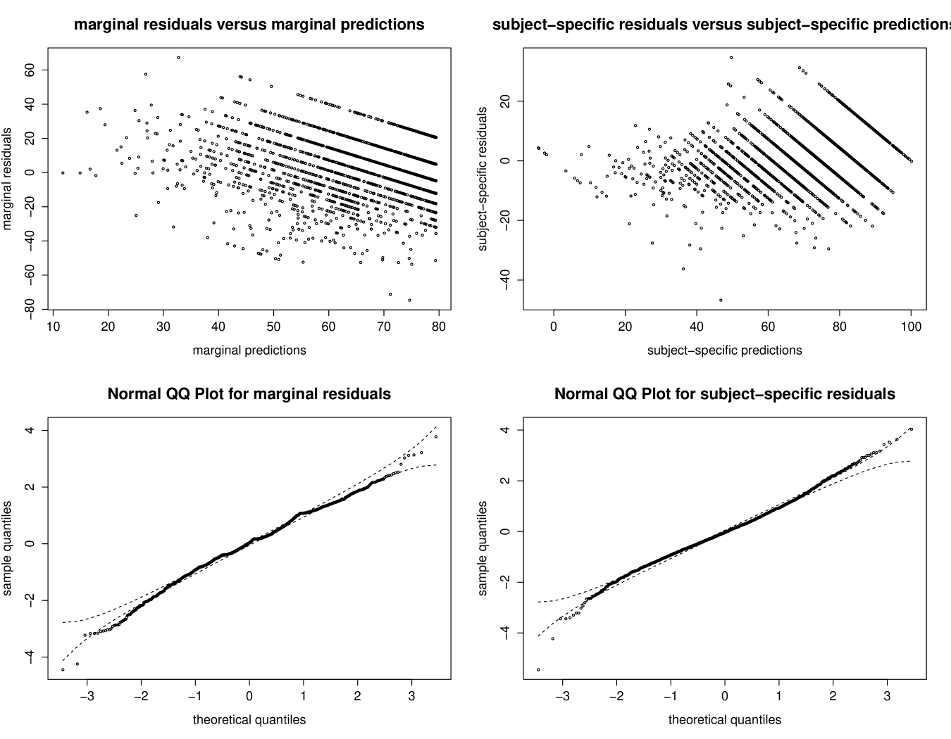
Figure 1: Subject-specific and marginal residuals in the two-class linear mixed model using plot.

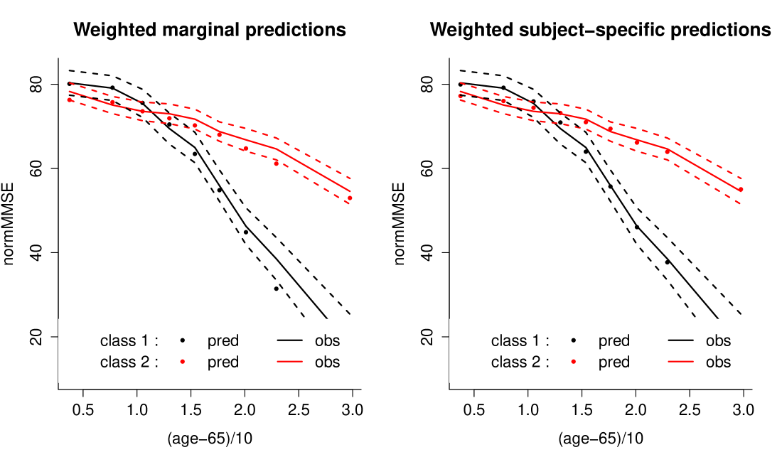
Figure 2: Weighted mean (marginal on the left, subject-specific on the right) predictions and weighted mean observations according to intervals of age in the two-class linear mixed model using plot and option which="fit".

Class-specific predictions, defined in Section 5.3, can be computed for any data contained in a dataframe as soon as all the covariates specified in the model are included in the dataframe. In the next lines, such a dataframe is created by generating a vector of age values between 65 and 95 and defining CEP at 1 or 0. The predictions are computed with predictY and plotted with the associated plot functionality or by using standard R tools as illustrated below and in Figure 3.

R> datnew <- data.frame(age = seq(65, 95, length = 100)) R> datnew$age65<-(datnew$age - 65) / 10 R> datnew$CEP<-0R>CEP0<-predictY(m2,datnew,var.time="age")R>datnew$CEP <- 1 R> CEP1 <- predictY(m2, datnew, var.time = "age") R> plot(CEP1, lty = 1,lwd = 2, type = "l", col = 1:2 , ylim = c(20, 100), + bty = "l", xlab = "age in year", ylab = "normalized MMSE", + legend = NULL) R> plot(CEP0, lty = 2, lwd = 2, type = "l", col = 1 : 2, ylim = c(20, 100), + add = TRUE) R> legend(x = "topright", bty = "n", ncol = 3, lty = c(NA, NA, 1, 1, 2, 2), + col = c(NA, NA, 1, 2, 1, 2), legend = c("G=1 (12.4+ "EL+", "EL+", "EL-", "EL-"), lwd = 2)

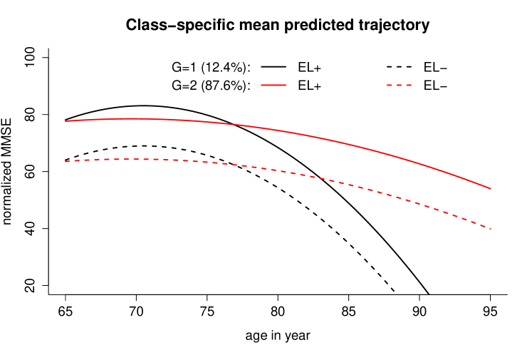
Figure 3: Predicted trajectories with age according to CEP in the two-class linear mixed model.

6.3 lcmm

The latent process mixed models implemented in lcmm are illustrated by the study of the linear trajectory of depressive symptoms (as measured by CES-D scale) with age65 adjusted for male and assuming correlated random effects for the intercept and age65. The next lines estimate the corresponding latent process mixed model with different link functions:

R> mlin <- lcmm(CESD   age65 * male, random =  age65, subject = ’ID’, + data = paquid) R> mbeta <- lcmm(CESD   age65 * male, random =  age65, subject = ’ID’, + data = paquid, link = ’beta’) R> mspl <- lcmm(CESD   age65 * male, random =  age65, subject = ’ID’, + data = paquid, link = ’splines’) R> mspl5q <- lcmm(CESD   age65 * male, random =  age65, subject = ’ID’, + data=paquid, link = ’5-quant-splines’)

Objects mlin, mbeta, mspl and mspl5q are latent process mixed models that assume the exact same trajectory for the underlying latent process but different link functions: linear, BetaCDF, I-splines with 5 equidistant knots (default with link=’splines’) and I-splines with 5 knots at percentiles, respectively. Note that mlin reduces to a standard linear mixed model (link=’linear’ by default). The only difference with a hlme object is the parameterization for the intercept and the residual standard error that are considered as rescaling parameters.

CES-D is an ordinal scale with more than 50 levels so it might be estimated with a cumulative probit mixed model, even if it is rarely done in practice because of the very high number of parameters induced as well as the substantial additional numerical complexity.

Owing to the numerical integration at each evaluation of the log-likelihood when assuming a threshold link function, estimation of the cumulative probit mixed model can be very long. We thus recommend estimating the model first without random effects to obtain satisfactory inital values for the thresholds before any inclusion of random effects, as shown in the next lines:

R> mord0 <- lcmm(CESD   age65 * male, random =  -1, subject = ’ID’, + data = paquid, link = ’thresholds’) R> binit <- NULL R> binit[1:6] <- mspl$best[1:6]R>binit[7:56]<-mord0$best[4:53] R> mord <- lcmm(CESD   age65 * male, random =  age65, subject = ’ID’, + data = paquid, link = ’thresholds’, B = binit)

Note here than mord takes a lot of time to be estimated (can be more than 1 hour depending on the computer).

The output of a lcmm object is very similar to that of a hlme object, as shown for mspl5q for example:

R> summary(mspl5q) General latent class mixed model fitted by maximum likelihood method

lcmm(fixed = CESD   age65 * male, random =  age65, subject = "ID", link = "5-quant-splines", data = paquid)

Statistical Model: Dataset: paquid Number of subjects: 500 Number of observations: 2104 Number of observations deleted: 146 Number of latent classes: 1 Number of parameters: 13 Link function: Quadratic I-splines with nodes 0 2 6 12 52

Iteration process: Convergence criteria satisfied Number of iterations: 19 Convergence criteria: parameters= 7.6e-09 : likelihood= 9.2e-08 : second derivatives= 1.8e-14

Goodness-of-fit statistics: maximum log-likelihood: -6320.08 AIC: 12666.17 BIC: 12720.96

Discrete posterior log-likelihood: -6309.09 Discrete AIC: 12644.18

Mean discrete AIC per subject: 12.6442 Mean UACV per subject: 12.6439 Mean discrete LL per subject: -12.6182

Maximum Likelihood Estimates:

Fixed effects in the longitudinal model:

coef Se Wald p-value intercept (not estimated) 0 age65 0.42421 0.06279 6.756 0.00000 male -0.83140 0.19742 -4.211 0.00003 age65:male 0.23371 0.10301 2.269 0.02327

Variance-covariance matrix of the random-effects: intercept age65 intercept 1.89911 age65 -0.39567 0.1711

Residual standard error (not estimated) = 1

Parameters of the link function:

coef Se Wald p-value I-splines1 -2.03816 0.13469 -15.132 0.00000 I-splines2 1.04627 0.02461 42.510 0.00000 I-splines3 0.74190 0.03773 19.665 0.00000 I-splines4 0.98399 0.03237 30.400 0.00000 I-splines5 1.55606 0.04480 34.735 0.00000 I-splines6 0.93273 0.16614 5.614 0.00000 I-splines7 1.38790 0.17687 7.847 0.00000

As mentionned earlier, the intercept of the latent process and the standard error of the measurement errors are respectively constrained to 0 and 1, and the parameters involved in the link functions are given at the end. Models involving discrete and continuous link functions can be compared using the discrete AIC provided in the summary. In this case, the model with a link function approximated by I-splines with 5 knots placed at the quantiles provides the best fit (12644.18 versus 12652.52 for the cumulative probit model, for example). To choose the optimal link function and further evaluate the nonlinearity of the relationship between the longitudinal marker and its underlying normal latent process, the estimated link functions are provided in output value estimlink and can be plotted as follows (plot in Figure 4). In this graph, confidence bands are obtained and plotted with function predictlink :

R> col <- rainbow(5) R> plot(mlin, which = "linkfunction", bty = ’l’, ylab = "CES-D", lwd = 2, + col = col[1], xlab = "underlying latent process") R> plot(mbeta, which = "linkfunction", add = T, col = col[2], lwd = 2) R> plot(mspl, which = "linkfunction", add = T, col = col[3], lwd = 2) R> plot(mspl5q, which = "linkfunction", add = T, col = col[4], lwd = 2) R> plot(mord, which = "linkfunction", add = T, col = col[5], lwd = 2) R> legend(x = "topleft", legend = c("linear", "beta", + "splines (5equidistant)", "splines (5 at quantiles)", "thresholds"), + lty = 1, col = col, bty = "n", lwd = 2) R> linkspl5q <- predictlink(mspl5q, ndraws = 2000) R> plot(linkspl5q, add = TRUE, col = col[4], lty = 2) R> legend(legend = c("95+ x = "left", lty = c(2, NA), col = c(col[4], NA), bty = "n", lwd = 1)

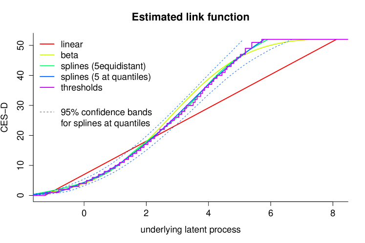
Figure 4: Estimated link functions for CES-D in a latent process mixed model using function plot with option which="linkfunction", and function predictlink: linear, Beta CDF, I-splines with 5 knots at quantiles or equidistant, and thresholds. 95% confidence bands are only given for the I-splines with 5 knots at quantiles.

As for hlme, plots for the residuals and the predictions versus observations can be provided but they are now in the latent process scale (only the code is provided here): R> plot(mspl5q) R> plot(mspl5q, which = "fit", var.time = "age65", xlab = "(age - 65) / 10", + bty = "l", break.times = 8, ylab = "latent process", lwd = 2, marg = F, + ylim = c(-1, 2))

Predictions in the latent process scale and in the outcome scale are computed according to a profile of covariates using respectively functions predictL and predictY at the maximum likelihood estimates or using a MonteCarlo method with argument draws=T (by default 2000 draws). The following lines give the code for computing the predictions in the original scale (CES-D):

R> datnew <- data.frame(age = seq(65, 95, length = 100)) R> datnew$age65<-(datnew$age - 65) / 10 R> datnew$male<-0R>women<-predictY(mspl5q,newdata=datnew,var.time="age",draws=T)R>datnew$male <- 1 R> men <- predictY(mspl5q, newdata = datnew, var.time = "age", draws = T)

The predicted trajectories can be plotted from these predictions as described below; the corresponding plot is displayed in Figure 5.

R> plot(women, lwd = c(2, 1), type = "l", col = 6, ylim = c(0, 20), + xlab = "age in year", ylab = "CES-D", bty = "l", legend = NULL) R> plot(men, add = TRUE, col = 4, lwd = c(2, 1)) R> legend(x = "topleft", bty = "n", ncol = 2, lty = c(1, 1, 2, 2), + col = c(6, 4, 6, 4), lwd = c(2, 2, 1, 1), + legend = c("women", "men", " 95

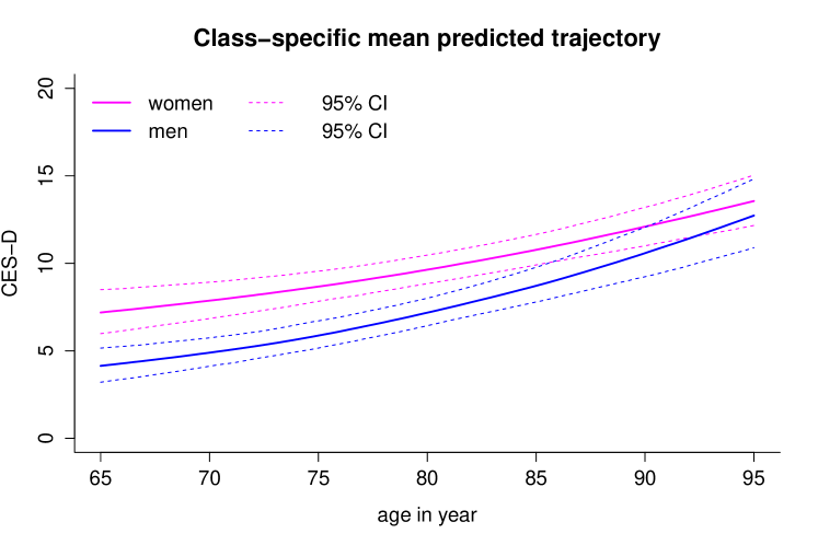
Figure 5: Predicted CES-D trajectories versus age according to gender with 95% confidence bands computed with function predictY.

In this example, only one latent class was assumed but a higher number of latent classes could be envisaged using the exact same syntax as shown in Section 6.2. The corresponding post-fit functions also apply with the same syntax.

6.4 multlcmm

The latent process mixed models for multivariate longitudinal data implemented in multlcmm are illustrated by the study of the quadratic trajectory with time of the global cognitive level defined as the common factor underlying three psychometric tests: MMSE, BVRT and IST. Here the timescale is years since entry into the cohort and the model is adjusted for age at entry. To further investigate the effect of gender, both an effect on the common factor and differential effects (contrasts) on each marker are included. Correlated random effects on the time functions are considered, as well as a Brownian motion with cor=BM(time) and a marker-specific random intercept with randomY=T. The next lines estimate the corresponding latent process mixed model with Beta CDF link functions and provide the summary output:

R> paquid$time<-(paquid$age - paquid$age_{i}nit)R>paquid$age0_centered <- paquid$age{}_{i}nit-75R>mult<-multlcmm(MMSE+IST+BVRTage0{}_{c}entered+male+contrast(male)++time+I(time{}^2/10),random=time+I(time{}^2/10),subject={}^{\prime }ID{}^{\prime }+,data=paquid,randomY=T,cor=BM(time),link=c({}^{\prime }beta{}^{\prime },{}^{\prime }beta{}^{\prime },+{}^{\prime }beta{}^{\prime }))R>summary(mult)Generallatentclassmixedmodelfittedbymaximumlikelihoodmethodmultlcmm(fixed=MMSE+IST+BVRTage0{}_{c}entered+male+contrast(male)+time+I(time{}^2/10),random=time+I(time{}^2/10),subject=\mathrm{"}ID\mathrm{"},randomY=T,link=c(\mathrm{"}beta\mathrm{"},\mathrm{"}beta\mathrm{"},\mathrm{"}beta\mathrm{"}),cor=BM(time),data=paquid)StatisticalModel:Dataset:paquidNumberofsubjects:500Numberofobservations:6216Numberoflatentclasses:1Numberofparameters:30Linkfunctions:StandardisedBetaCdFforMMSEStandardisedBetaCdFforISTStandardisedBetaCdFforBVRTIterationprocess:ConvergencecriteriasatisfiedNumberofiterations:16Convergencecriteria:parameters=1.2e-10:likelihood=1.1e-08:secondderivatives=3.6e-13Goodness-of-fitstatistics:maximumlog-likelihood:-14374.6AIC:28809.21BIC:28935.65MaximumLikelihoodEstimates:Fixedeffectsinthelongitudinalmodel:coefSeWaldp-valueintercept(notestimated)0.00000age0{}_{c}entered-\mathrm{0.109410.01133}-\mathrm{9.6570.00000}male\mathrm{0.147550.118821.2420.21431}time-\mathrm{0.122260.01878}-\mathrm{6.5110.00000}I(time{}^2/10)-\mathrm{0.023960.00975}-\mathrm{2.4590.01394}Contrastsonmale(p=0.00027)MMSE-\mathrm{0.074820.06917}-\mathrm{1.0820.27940}IST-\mathrm{0.268140.07853}-\mathrm{3.4150.00064}BVRT\ast \ast \mathrm{0.342960.088073.8940.00010}Variance-covariancematrixoftherandom-effects:(thevarianceofthefirstrandomeffectisnotestimated)intercepttimeI(time{}^2/10)intercept1.00000time\mathrm{0.003850.01399}I(time{}^2/10)-0.00729-\mathrm{0.004670.00298}coefSeBMstandarderror:\mathrm{0.308560.04186}MMSEISTBVRTResidualstandarderror:\mathrm{1.013690.928301.42295}Standarderroroftherandomeffect:\mathrm{0.574990.853640.88877}Parametersofthelinkfunctions:coefSeWaldp-valueMMSE-Beta\mathrm{11.420400.0711419.9660.00000}MMSE-Beta2-\mathrm{0.246910.08368}-\mathrm{2.9510.00317}MMSE-Beta\mathrm{30.456130.0260317.5210.00000}MMSE-Beta\mathrm{40.064580.0058011.1250.00000}IST-Beta1-\mathrm{0.036940.05647}-\mathrm{0.6540.51295}IST-Beta2-\mathrm{0.421830.07554}-\mathrm{5.5840.00000}IST-Beta\mathrm{30.651920.0156141.7760.00000}IST-Beta\mathrm{40.082940.0067612.2620.00000}BVRT-Beta\mathrm{10.401650.080634.9820.00000}BVRT-Beta2-\mathrm{0.263900.12251}-\mathrm{2.1540.03124}BVRT-Beta\mathrm{30.557310.0197728.1850.00000}BVRT-Beta\mathrm{40.062900.006329.9520.00000}\ast \ast coefficientnotestimatedbutobtainedfromtheothersasminusthesumofthemInthisexample,squaredtimewasdividedby10inordertoavoidverysmallnumbersforthecorrespondingfixedeffectandvarianceoftherandomeffect.Thesummaryhasthesameappearanceasthesummariesofhlmeorlcmmobjects.Inadditiontothefixedeffectsonthelatentprocess(commonfactor),themarker-specificcontrastsaregivenandtheirglobalsignificanceistestedwithamultivariateWaldtest.Thentheestimatedvariance-covarianceoftherandomeffectsandthestandarderrorofthemarker-specificintercept(\mathrm{"}\text{Standard error of the random effect}\mathrm{"})aregivenalongwiththestandarderroroftheindependentGaussianerror(\mathrm{"}\text{Residual standard error}\mathrm{"}).Finally,themarker-specificlinkfunctionparametersareprovided.Notethatinmultlcmm,theinterceptofthelatentprocessandthevarianceoftherandominterceptarerespectivelyconstrainedto0and1.Asforlcmmobject,theestimatedlinkfunctioncanbeplottedwithfunctionplotandoption\mathrm{"}linkfunction\mathrm{"}orwiththe95\%confidencebandsusingpredictlinkasshownbelowandinFigure\text{<a href="\#S6.F6" title="Figure 6 ‣ 6.4 codemultlcmm ‣ 6 Examples ‣ Estimation of Extended Mixed Models Using Latent Classes and Latent Processes: The proglangR Package pkglcmm" class="ltx\_ref ltx\_font\_italic"><span class="ltx\_text ltx\_ref\_tag">6</span></a>}:R>plot(mult,which=\mathrm{"}linkfunction\mathrm{"},col=c(1,4,6),lwd=2)R>CI<-predictlink(mult)R>plot(CI,col=c(1,4,6),lwd=2)R>head(CIpred)YnameYvaluestransfY{}_{5}0transfY{}_2.5transfY{}_{9}7.51MMSE0.0000000-7.039481-8.272866-6.0885532MMSE0.3030303-7.005178-8.214649-6.0620413MMSE0.6060606-6.969232-8.158112-6.0405324MMSE0.9090909-6.931033-8.103282-6.0063055MMSE1.2121212-6.895605-8.055205-5.9753746MMSE1.5151515-6.856988-8.010372-5.949715Noteherethatthepredictedvaluesofthelinkfunctionsshownabovearethemedian(50\%),and2.5\%,97.5\%of2000drawsgeneratedfromtheasymptoticdistribution.Assuch,theymayvarydependingontheseed.\text{Figure 6Figure 66Figure 66Estimatedlinkfunctio}$