Detecting communities using asymptotical surprise

Abstract

Nodes in real-world networks are repeatedly observed to form dense clusters, often referred to as communities. Methods to detect these groups of nodes usually maximize an objective function, which implicitly contains the definition of a community. We here analyze a recently proposed measure called surprise, which assesses the quality of the partition of a network into communities. In its current form, the formulation of surprise is rather difficult to analyze. We here therefore develop an accurate asymptotic approximation. This allows for the development of an efficient algorithm for optimizing surprise. Incidentally, this leads to a straightforward extension of surprise to weighted graphs. Additionally, the approximation makes it possible to analyze surprise more closely and compare it to other methods, especially modularity. We show that surprise is (nearly) unaffected by the well known resolution limit, a particular problem for modularity. However, surprise may tend to overestimate the number of communities, whereas they may be underestimated by modularity. In short, surprise works well in the limit of many small communities, whereas modularity works better in the limit of few large communities. In this sense, surprise is more discriminative than modularity, and may find communities where modularity fails to discern any structure.

I Introduction

Networks are often used as a model to describe interactions among components of a system Albert and Barabási (2002); Dorogovtsev (2010). In its simplest form, a network is composed of a set of vertices (also called nodes) and a set of edges connecting them. Many real-world systems can be reduced to this scheme, such as social networks establishing relations among individuals, proteins interacting within the cell or roads connecting different cities Newman (2010). What caught the interest of the scientific community was that most of these real networks share high-order structural patterns and dynamics, such as a wide heterogeneity in the number of neighbors of a node, the presence of many triangles or a very low network diameter Barabási and Albert (1999); Watts and Strogatz (1998). Another feature observed in real networks is the presence of densely connected groups of nodes, known as communities Fortunato (2010). Nodes in the same group usually share similar characteristics or functions and, therefore, methods to detect communities in networks are of much interest across different fields Girvan and Newman (2002); Gleiser and Danon (2003); Palla and Dere (2005); Guimerà et al. (2005); Olesen et al. (2007); Lupu and Traag (2013)

Researchers have proposed numerous strategies to detect the community structure of a network Danon, D, and Duch (2005); Lancichinetti et al. (2011); Fortunato (2010); Aldecoa and Marín (2013a). Ultimately, most methods optimize a given objective function to find a partition into communities. This function contains, either explicitly or implicitly, its own definition of a community. Modularity Newman and Girvan (2004) has been, since its inception, the most extensively used measure for community detection. It belongs to a wider class of functions in which communities are defined by Potts model spin states and the quality of the partition is given by the energy of the system Reichardt and Bornholdt (2006); Ronhovde and Nussinov (2010). Although this approach based on statistical mechanics may be appealing, empirical evidence shows that in many cases these methods are unable to capture the expected communities of the network Lancichinetti and Fortunato (2009); Good, de Montjoye, and Clauset (2010); Aldecoa and Marín (2013b, a); Traag, Krings, and Van Dooren (2013). In fact, numerous studies have pointed out strong theoretical limitations of modularity approaches for community detection Fortunato and Barthélemy (2007); Kumpula et al. (2007); Lancichinetti and Fortunato (2011); Bagrow (2012); Xiang and Hu (2012); Kehagias (2012); Traag, Van Dooren, and Nesterov (2011).

A proposed measure based on classical probability, called surprise Aldecoa and Marín (2011), has been shown to systematically outperform modularity-based methods on different benchmarks Aldecoa and Marín (2013b, a). Here we demonstrate how surprise can be expressed under an information-theoretic framework, by examining its asymptotic formulation. In particular, we describe surprise in terms of the Kullback-Leibler (KL) divergence Kullback and Leibler (1951). This asymptotic formulation allows us to develop, for the first time, an efficient surprise maximization algorithm. Incidentally, this also points to a straightforward extension of surprise to weighted graphs. Additionally, this enables a better analysis of its performance, and allows an analytic comparison to other methods.

In particular, we compare surprise to a modularity model and the recently introduced measure of significance, which also detects communities based on the KL-divergence Traag, Krings, and Van Dooren (2013). We show that surprise is more discriminative than modularity using an Erdös-Rényi (ER) null model, and that significance and surprise behave relatively similar. Additionally, we analyze the limitations of community detection, most notably the resolution limit Fortunato and Barthélemy (2007) and the detectability threshold Decelle et al. (2011). We show that surprise is (nearly) unaffected by the resolution limit, and works well in the limit of large number of communities with fixed community sizes. However, in the limit of large community sizes with a fixed number of communities, surprise works worse than ER modularity, as it tends to find smaller subgraphs within those larger communities.

Apart from the choice of the null model, a key component in community detection is how the difference between the actual community structure and the null model is quantified. Relying on the KL-divergence to measure such difference results in more discriminative methods. We believe that this fact can improve current and future community detection strategies.

II Surprise

In general, we denote a graph by $G=(V,E)$ consisting of nodes $V=\{1,\ldots,n\}$ and edges $E\subseteq V\times V$, which has $n=|V|$ nodes and $m=|E|$ links. The total number of possible links is denoted by $M=\binom{n}{2}$, and the ratio of present links $p=\frac{m}{M}$ is known as the density of the graph.

The general aim is to find a good partition $\mathcal{V}=\{V_{1},V_{2},\ldots,V_{r}\}$ of the graph, where each $V_{c}\subseteq V$ is a set of nodes, which we call a community. Such communities are non-overlapping (i.e. $V_{c}\cap V_{d}=\emptyset$ for all $c\neq d$) and cover all the nodes (i.e. $\bigcup V_{c}=V$). Each community consists of $n_{c}=|V_{c}|$ nodes and contains $m_{c}=|E_{c}|$edges. Obviously then $\sum_{c}n_{c}=n$, but the total number of internal edges $m_{\text{int}}=\sum_{c}m_{c}$ is smaller than the total number of edges so that $m_{\text{int}}\leq m$. An overview of the relevant variables is provided in Table 1.

Graph variables
$n$	Number of nodes
$m$	Number of edges
$M=\binom{n}{2}$	Number of possible edges
$p=\frac{m}{M}$	Density
Community variables
$n_{c}$	Number of nodes in community $c$
$m_{c}$	Number of edges in community $c$
$\langle m_{c}\rangle$	Expected number of edges in community $c$
$p_{c}=\frac{m_{c}}{\binom{n_{c}}{2}}$	Density of community $c$
Partition variables
$m_{\text{int}}=\sum_{c}m_{c}$	Total internal edges
$M_{\text{int}}=\sum_{c}\binom{n_{c}}{2}$	Total possible internal edges
$q=\frac{m_{\text{int}}}{m}$	Fraction of internal edges
$\langle q\rangle=\frac{M_{\text{int}}}{M}$	Expected fraction of internal edges

Table 1: Variables.

Surprise is a statistical approach to assess the quality of a partition into communities. Given a graph with $n$ nodes, there are $M=\binom{n}{2}$ possible ways of drawing $m$ edges. Out of those, there are $M_{\text{int}}=\sum_{c}\binom{n_{c}}{2}$ possible ways of drawing an internal edge. Surprise is then defined as the (minus logarithm of the) probability of observing at least $m_{\text{int}}$ successes (internal edges) in $m$ draws without replacement from a finite population of size $M$ containing exactly $M_{\text{int}}$ possible successes Arnau, Mars, and Marín (2005); Aldecoa and Marín (2011):

$$\mathcal{S}(\mathcal{V})=-\log\sum_{i=m_{\text{int}}}^{\min(m,M_{\text{int}})}\frac{\displaystyle\binom{M_{\text{int}}}{i}\binom{M-M_{\text{int}}}{m-i}}{\displaystyle{\binom{M}{m}}},$$ (1)

which derives from the hypergeometric distribution.

II.0.1 Asymptotic formulation

However, this formulation presents some difficulties. It is not straightforward to work with, nor is it simple to implement in an optimization procedure, mainly due to numerical computational problems. Since we are usually interested in relatively large graphs, an asymptotic approximation may provide a good alternative. The asymptotic expansion we consider here assumes that the graph grows, but that the relative number of internal edges $q=\frac{m_{\text{int}}}{m}$ and the relative number of expected internal edges $\langle q\rangle=\frac{M_{\text{int}}}{M}$ remains fixed. By only considering the dominant term, we obtain a simple and elegant approximation (see Appendix A)

$$\mathcal{S}(\mathcal{V})\approx mD(q\parallel\langle q\rangle),$$ (2)

where $D(x\parallel y)$ is the KL divergence

$$D(x\parallel y)=x\log\frac{x}{y}+(1-x)\log\frac{1-x}{1-y}.$$ (3)

The KL divergence measures the distance between two probability distributions (although it is not a proper metric), with in this case the Bernoulli probability distributions $x$, $1-x$ and $y$, $1-y$. Notice that, in general, $D(x\parallel y)\neq D(y\parallel x)$. In this case, $q$ and $\langle q\rangle$ denote the probability that a link lies (or is expected to lie) within a community. Whenever $q=\langle q\rangle$, we have that $D(q\parallel\langle q\rangle)=0$ and, otherwise, $D(q\parallel\langle q\rangle)>0$. Since we are looking for relatively dense communities, we generally have $q>\langle q\rangle$.

The original formulation of surprise in Eq. (1), based on a hypergeometric distribution, can be accurately approximated by a binomial distribution. The only difference between both approaches is that in the former links are drawn without replacement. Consider again $q=\frac{m_{\text{int}}}{m}$, the fraction of internal edges in the partition, and $\langle q\rangle=\frac{M_{\text{int}}}{M}$, the expected fraction of internal edges. The binomial formulation of surprise would then be

$$\mathcal{S}(\mathcal{V})=-\log\sum_{i=m_{\text{int}}}^{\min(m,M_{\text{int}})}\binom{m}{i}\,\langle q\rangle^{i}\,(1-\langle q\rangle)^{m-i}$$ (4)

The asymptotic development for the dominant term of binomial surprise is simpler. We use Stirling’s approximation,

$$\log{\binom{n}{k}}\approx n\,H\left(\frac{k}{n}\right)$$ (5)

where $H(x)=-x\log x-(1-x)\log(1-x)$ is the (binary) entropy and we use that $m_{\text{int}}=qm$. Binomial surprise then becomes

$$\mathcal{S}(\mathcal{V}) \approx-m\Bigl{[}H(q)+q\log\langle q\rangle+(1-q)\log(1-\langle q\rangle)\Bigr{]}$$

$$=mD(q\parallel\langle q\rangle)$$

Thus, as expected, for large sparse networks the difference between drawing with or without replacement is negligible.

II.0.2 Algorithm

Evaluating the quality of a partition using surprise shows excellent results in standard benchmarks. In fact, it has been shown that a meta-algorithm of selecting the partition with the highest surprise, from a set of candidate solutions provided by the best community detection algorithm solutions, outperforms any single algorithm by itself Aldecoa and Marín (2013b, a, 2014). However, no algorithm for directly optimizing surprise has been developed yet.

The asymptotic formulation allows a straightforward algorithmic implementation, in a similar fashion as the Louvain algorithm Blondel et al. (2008), which was initially designed to optimize modularity. The basic idea of the Louvain algorithm consists of two steps. We move around nodes from one community to another so as to greedily improve surprise. When surprise can no longer be improved by moving around individual nodes, we aggregate the graph, and repeat the procedure on the aggregated graph.

The aggregation of the graph is simply the contraction of all nodes within a community to a single “community node”. The multiplicities of the edges are kept as weighted edges, so that $w_{cd}=\sum_{i\in V_{c},j\in V_{d}}w_{ij}$ denotes the weight between the new nodes $c$ and $d$ in the aggregate graph, where initially $w_{ij}=A_{ij}$. Here, $A_{ij}=1$ if there is an edge between $i$ and $j$, and $0$ otherwise. We additionally need a node size to keep track of the total size of the communities, similar to Traag, Van Dooren, and Nesterov (2011). Initially we set this node size to $n_{i}=1$, and upon aggregation the node size $n_{c}=\sum_{i\in V_{c}}n_{i}$ is set to the total number of nodes within the community.

One of the essential elements of the Louvain algorithm is that the surprise of the partition on the aggregated graph is the same as the surprise of the original partition on the original graph. This ensures that moving a node in the aggregated graph corresponds to moving a whole community in the original graph. In other words, if $\mathcal{V}$ denotes the partition of $G$ and $\mathcal{V}^{\prime}=\{1,2,\ldots,r\}$ denotes the default partition of the aggregated graph $G^{\prime}$, then $\mathcal{S}(\mathcal{V},G)=\mathcal{S}(\mathcal{V}^{\prime},G^{\prime})$. For calculating surprise in the aggregated graph, we then use $m_{c}=\sum_{i,j\in V^{\prime}_{c}}w^{\prime}_{ij}$ as the internal weight and $n_{c}=\sum_{i\in V^{\prime}_{c}}n_{i}$ as the community size and $n=\sum_{c}n_{c}$. With the other definitions remaining the same, it is straightforward to see that $\mathcal{S}(\mathcal{V},G)=\mathcal{S}(\mathcal{V}^{\prime},G^{\prime})$. Notice that the same formulations can also be applied to the original graph, when using $w_{ij}=A_{ij}$ and $n_{i}=1$.

Using this formulation of the aggregate graph, it is quite straightforward to calculate the improvement in surprise when moving a node. Before we move node $i$ from community $c$ to community $d$, assume we have $m_{\text{int}}$ internal edges, and $M_{\text{int}}$ possible internal edges. The total weight between node $i$ and community $c$ is $w_{ic}=\sum_{j\neq i\in V_{c}}w_{ij}$ and similarly between node $i$ and community $d$, with a possible self-loop of $w_{ii}$. The new internal weight after moving node $i$ from community $c$ to community $d$ is then $m^{\prime}_{\text{int}}=m_{\text{int}}-w_{ic}+w_{id}$. The change in $M_{\text{int}}=\sum_{c}\binom{n_{c}}{2}$ is slightly more complicated. After the move, we obtain $n^{\prime}_{c}=n_{c}-n_{i}$ and $n^{\prime}_{d}=n_{d}+n_{i}$, so that $M^{\prime}_{\text{int}}=M_{\text{int}}+n_{i}(n_{i}+n_{d}-n_{c})$. Finally, we use $q^{\prime}=\frac{m^{\prime}_{\text{int}}}{m}$ and $\langle q^{\prime}\rangle=\frac{M^{\prime}_{\text{int}}}{M}$. The difference in surprise for moving node $i$ from community $c$ to community $d$ is then simply

$$\Delta\mathcal{S}(\sigma_{i}=c\mapsto d)=m\left(D(q\parallel\langle q\rangle)-D(q^{\prime}\parallel\langle q^{\prime}\rangle)\right),$$ (6)

where we denote the community of node $i$ by $\sigma_{i}$ (i.e. $\sigma_{i}=c$ if $i\in V_{c}$). The algorithm can then be simply summarized as follows:

function Optimizesurprise(Graph $G$)

     while improvement do

         $\sigma_{i}\leftarrow i$ for $i=1,\ldots,|V(G)|$. $\triangleright$ Initial partition

         while improvement do

              for random $v\in V(G)$ do

                  $\sigma_{v}\leftarrow\operatorname*{arg\,max}_{d}\Delta\mathcal{S}(\sigma_{v}=c\mapsto d)$

              end for

         end while

         $\sigma^{\prime}_{i}=\sigma_{\sigma^{\prime}_{i}}$ $\triangleright$ Community in original graph.

         $G\leftarrow$ AggregateGraph($G$)

     end while

     return $\sigma^{\prime}$

end function

Incidentally, our formulation for surprise for the aggregated graph yields a weighted version of surprise. While keeping the same formulation of surprise as in Eq. (2), we only need to change the definitions of $q$ and $\langle q\rangle$. Then $q=\sum_{c}w_{c}/w$ where $w_{c}=\sum_{i,j\in V_{c}}w_{ij}$ is the internal weight and $w=\sum_{ij}w_{ij}$ is the total weight. Assuming then a uniform distribution of weights across the graph in the random graph, the expected weights of an edge would be $\langle w\rangle$, which would not show too much deviation. The total possible internal weight is then $\langle w\rangle M_{\text{int}}$, while the total possible weight would be $\langle w\rangle M$. Hence, $\langle q\rangle=M_{\text{int}}/M$ remains unchanged.

We provide an open-source, fast and flexible C++ implementation of the optimization of surprise using the Louvain algorithm. It is suitable for use in python using the igraph package. This implementation is available from GitHub as louvain-igraph and from PyPi simply as louvain and implements various other methods as well.

III Comparison

We now review how surprise compares to some closely related methods. There are many other methods still, and we cannot do all of them justice here. For a more comprehensive review, please refer to Fortunato (2010); Porter, Onnela, and Mucha (2009).

III.1 Modularity

Although relatively recent, modularity has rapidly become an extremely popular method for community detection. The general idea is that we want to find a partition, such that the communities have more internal links than expected. In its original formulation, modularity assumes a null model in which the degree $k_{i}$ of a node is fixed Newman and Girvan (2004), the so called configuration model Molloy and Reed (1995). This implies that the expected number of internal edges is

$$\langle m_{c}\rangle=\frac{K_{c}^{2}}{4m},$$ (7)

where $K_{c}=\sum_{i\in V_{c}}k_{i}$ is the total degree of nodes in community $c$. Modularity compares this value to the observed number of edges $m_{c}$ within the community, and simply sums the difference. The measure is usually normalized by the total number of edges, obtaining

$$\mathcal{Q}_{\text{CM}}(\mathcal{V})=\frac{1}{m}\sum_{c}\left(m_{c}-\frac{K_{c}^{2}}{4m}\right).$$ (8)

This random graph null model represents the configuration model, where the degree dependency of the nodes is taken into account. We therefore refer to it as the CM modularity.

Alternative derivations of modularity have been proposed, some of them with different null models Reichardt and Bornholdt (2006). Surprise implicitly assumes a null model in which every edge appears with the same probability $p$, as in an ER random graph. The number of expected edges in a community of size $c$ is thus

$$\langle m_{c}\rangle=p\binom{n_{c}}{2}.$$ (9)

Plugging this null model into modularity, we obtain its ER version Reichardt and Bornholdt (2006)

$$\mathcal{Q}_{\text{ER}}(\mathcal{V})=\frac{1}{m}\sum_{c}\left(m_{c}-p\binom{n_{c}}{2}\right),$$ (10)

There is an interesting relationship between this ER modularity and surprise. Given that $p=m/M$, we can write

$$\mathcal{Q}_{\text{ER}}(\mathcal{V}) =\sum_{c}\frac{m_{c}}{m}-\sum_{c}\frac{\binom{n_{c}}{2}}{M}$$ (11)

$$=q-\langle q\rangle.$$ (12)

By Pinsker’s inequality this is related to the KL divergence as

$$q-\langle q\rangle\leq\sqrt{\frac{1}{2}D(q\parallel\langle q\rangle)},$$ (13)

and, therefore,

$$\mathcal{S}(\mathcal{V})=mD(q\parallel\langle q\rangle)\geq 2m\mathcal{Q}_{\text{ER}}(\mathcal{V})^{2}.$$ (14)

This implies that whenever surprise is low, modularity is also low. Whenever a good partition (in the sense of being different from random) cannot be found by surprise, it is unlikely that modularity will be able to find one. While Eq. (14) is sometimes tight, on some partitions surprise can be much larger than modularity, making it more likely to be selected as optimal while escaping the scrutiny of modularity optimization. In this sense, surprise is more discriminative than modularity

To illustrate this, consider a one dimensional circular lattice with neighbors within distance $3$. In other words, node $i$ is connected to nodes $i-3\mod n$ to $i+3\mod n$ (excluding the self-loop). We create partitions consisting of $r$ communities by grouping consecutive nodes such that $n/r$ nodes are in the same community. The ER modularity reaches its maximum with just a few communities (Fig. 1). Modularity indeed often detects only few communities, part of the problem of its resolution limit Fortunato and Barthélemy (2007); Kumpula et al. (2007); Traag, Van Dooren, and Nesterov (2011). Both surprise and significance (see next section), still increase whereas ER modularity is already decreasing again. ER modularity may not be able to discern partitions with many communities, whereas surprise and significance can. On the other hand, when surprise goes to $0$ we see that ER modularity indeed also goes to $0$, showing the upper bound provided by surprise.

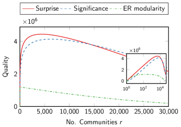
Figure 1: (Color online) Comparison of bounds. We show the quality of partitions of a lattice in $r$ communities. ER modularity quickly reaches a maximum for few communities (we show $2mQ_{\text{ER}}^{2}$ rather than $Q_{\text{ER}}$ for comparison). Both significance and surprise reach a maximum for much more communities. This illustrates that ER modularity is simply unable to discern partitions with such a high number of communities. The inset shows the same data, but on a logarithmic x-axis.

III.2 Significance

Significance Traag, Krings, and Van Dooren (2013), a recently introduced objective function to evaluate community structure quality, presents an approach similar to surprise. Surprise describes how likely it is to observe $m_{\text{int}}$ internal links in communities. Significance, on the other hand, looks at how likely such dense communities appear in a random graph. Comparing the two measures is not immediately straightforward. On the one hand, if dense communities are unlikely to be present in a random graph (high significance), then a community is also unlikely to contain many links at random (high surprise). On the other hand, if a community is unlikely to contain many links at random (high surprise), perhaps there are still communities elsewhere in the random graph that contain so many links. Therefore we should compare the two more formally to make more exact statements.

Asymptotically, significance is defined as

$$\mathcal{Z}(\mathcal{V})=\sum_{c}\binom{n_{c}}{2}D(p_{c}\parallel p),$$ (15)

where $p_{c}=m_{c}/\binom{n_{c}}{2}$ is the density of community $c$, $p$ is the density of the graph and $D(x\parallel y)$ is again the KL divergence. Significance also showed a great performance in standard benchmarks, and helped to determine the proper scale of resolution in multi-resolution methods Traag, Krings, and Van Dooren (2013).

Both surprise and significance are based on the KL divergence to compare the actual number of internal edges to the expected one. However, they do so in different ways. Whereas surprise compares such difference using global quantities, $q$ and $\langle q\rangle$, significance compares each community density $p_{c}$ to the average graph density $p$.

This implies, among other things, that only significance is affected by the actual distribution of edges between communities. In particular, moving edges from a denser community (with a high $p_{c}$) to a sparse community (with a low $p_{c}$), generally decreases the value of significance. This means that if all communities have the same density, ceteris paribus, significance is minimal. This intuition is confirmed by convexity of the KL divergence (see Appendix B), so that significance is lower-bounded by

$$\mathcal{Z}(\mathcal{V})\geq M_{\text{int}}D(\langle p_{c}\rangle\parallel p)$$ (16)

with the weighted average density

$$\langle p_{c}\rangle=\sum_{c}\frac{\binom{n_{c}}{2}}{M_{\text{int}}}p_{c}=\frac{m_{\text{int}}}{M_{\text{int}}}=p\frac{q}{\langle q\rangle}.$$ (17)

Convexity of the KL divergence, also shows that

$$\mathcal{Z}(\mathcal{V}) \geq\mathcal{S}(\mathcal{V})$$ (18)

whenever $\langle q\rangle<p$ (see Appendix B). To gain more insight, we can slightly rewrite $\langle q\rangle$ to obtain

$$\langle q\rangle=\frac{\sum_{c}\binom{n_{c}}{2}}{\binom{n}{2}}\approx\frac{\sum_{c}n_{c}^{2}}{n^{2}}=\frac{1}{r}\frac{\langle n_{c}^{2}\rangle}{\langle n_{c}\rangle^{2}}.$$ (19)

Then, in general, $\langle q\rangle$ will be inversely proportional to the number of communities, and increases with the variance of the community sizes $n_{c}$. Hence, if the number of communities is relatively large (small $\langle q\rangle$), or the network is relatively dense (large $p$), significance is more discriminative than surprise. However, in the case that $\langle q\rangle>p$, surprise can be more discriminative than significance (see appendix B). Notice that if $\langle q\rangle=p$, then $p_{c}=q$, so that $D(\langle p_{c}\rangle\parallel p)=D(q\parallel\langle q\rangle)$ and significance and surprise values are close to each other. Therefore, the two measures are expected to behave relatively similar, especially for $\langle q\rangle\approx p$. Nonetheless, in dense networks with many communities significance would be more discriminative, whereas for fewer communities or sparse graphs, surprise would show a better performance.

IV Limitations

Although modularity was lauded by the possibility to detect communities without specifying the number of communities, this came at a certain price. One of the best known problems in community detection is the resolution limit Fortunato and Barthélemy (2007), which prevents modularity from detecting small communities. It thus tends to underestimate the number of communities in a graph, and lumps together several smaller communities in larger communities. Moreover, this depends on the scale of the graph, so that modularity has a problem of scale. It was shown that this is the case for both ER and CM modularity, and that other null models also suffer from the same drawbacks Kumpula et al. (2007). In fact, most methods are expected to suffer from this problem, and only few methods are able to avoid it completely Traag, Van Dooren, and Nesterov (2011). Additionally, there is also a lower counterpart to the resolution limit, leading to unnecessary splitting of cliques Krings and Blondel (2011); Traag (2014). Finally, modularity is also myopic, cutting across long dendrites Schaub et al. (2012). Another fundamental limit in community detection is called the detectability threshold Decelle et al. (2011), which also has some counter-intuitive effects Radicchi (2014). This prevents any method from correctly detecting communities beyond this threshold. The asymptotic formulation of surprise enables us to understand better how it performs with respect to these limitations.

IV.1 Resolution limit

The resolution limit is traditionally studied through the ring of cliques Fortunato and Barthélemy (2007). This is a graph consisting of $r$ cliques (i.e. completely connected subgraphs) connected only by one link between two cliques to form a ring. This is one of the most modular structure possible: we cannot delete more than one link between communities and still keep it connected, while we cannot add any more links within the cliques. When a method starts to join the cliques, it can no longer detect the smaller cliques, and so a fortiori, cannot detect less well defined subgraphs either. We denote by $q_{1}$ (and $\langle q_{1}\rangle$) the (expected) proportion of edges within communities for the partition where each community contains a single clique and use $q_{2}$ (and $\langle q_{2}\rangle$) for the partition where each community contains two cliques. To facilitate the derivation, we work with self-loops (and directed edges), so that the total number of edges is $n_{c}^{2}$ within communities respectively. Let $r$ denote the number of cliques. Then obviously $n=rn_{c}$ and $m=rn_{c}^{2}+2r$. For the partition of each clique in its own community we then obtain

$$q_{1} =\frac{n_{c}^{2}}{n_{c}^{2}+2}, \langle q_{1}\rangle =\frac{1}{r},$$ (20)

while for the partition with $2$ cliques merged we obtain

$$q_{2} =\frac{n_{c}^{2}+1}{n_{c}^{2}+2}, \langle q_{2}\rangle =\frac{2}{r}.$$ (21)

Hence, $q_{2}=q_{1}+\epsilon$ with $\epsilon=\frac{1}{n_{c}^{2}+2}$ and $\langle q_{2}\rangle=2\langle q_{1}\rangle$. The difference of surprise is

$$\Delta\mathcal{S}=\frac{\mathcal{S}_{2}-\mathcal{S}_{1}}{m}=D(q_{2}\parallel\langle q_{2}\rangle)-D(q_{1}\parallel\langle q_{1}\rangle)$$ (22)

which works out to

$$\Delta\mathcal{S}=q_{1}\log\frac{q_{2}}{\langle q_{2}\rangle}\frac{\langle q_{1}\rangle}{q_{1}}+(1-q_{1})\log\frac{1-q_{2}}{1-\langle q_{2}\rangle}\frac{1-\langle q_{1}\rangle}{1-q_{1}}+\\ \epsilon\log\frac{q_{2}}{\langle q_{2}\rangle}\frac{1-\langle q_{2}\rangle}{1-q_{2}}.$$ (23)

Approximating $r-2\approx r-1\approx r$ we obtain

$$\Delta\mathcal{S}\approx-D(q_{1}\parallel q_{2})-q_{1}\log 2+\epsilon\log\frac{r}{2}\frac{q_{2}}{1-q_{2}}.$$ (24)

Solving for $r$ at the point at which $\Delta\mathcal{S}=0$ yields

$$r=2\frac{1-q_{2}}{q_{2}}\exp\left(\frac{1}{\epsilon}D(q_{1}\parallel q_{2})\right)2^{\frac{q_{1}}{\epsilon}}$$ (25)

which scales as $r\sim\frac{2^{n_{c}^{2}}}{n_{c}^{2}}$ so that for larger $r$ surprise starts to merge cliques.

Working out the inequality for both CM and ER modularity we obtain that $r\sim n_{c}^{2}$. Hence, the number of cliques $r$ at which modularity starts to merge cliques lies considerably lower than for surprise and grows linearly with the square of community sizes rather than exponentially. So, although surprise shows a similar problem as modularity, it only starts to show at really large graphs, so is unlikely to be a problem in any empirical graph. Indeed, this demonstrates exactly the key difference between modularity and surprise: The first is unable to detect relatively small communities in large graphs, whereas the latter has (nearly) no such difficulties.

IV.2 Detectability threshold

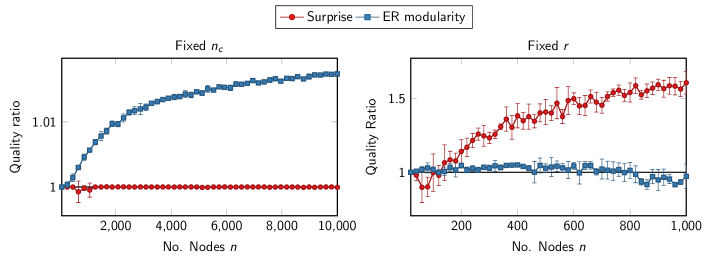
Figure 2: (Color online) Limitations on community detection. We construct graphs with a planted partition, with a probability of an edge between communities of $\mu=0.1$. We show the quality ratio $\frac{\mathcal{S}}{\mathcal{S}_{\text{plt}}}$ between the quality of the partition found by optimization $\mathcal{S}$ and the quality of the planted partition $\mathcal{S}_{\text{plt}}$ (and similarly for ER modularity). Hence, if the quality ratio $\frac{\mathcal{S}}{\mathcal{S}_{\text{plt}}}>1$, the planted partition is no longer optimal. In the figure on the left we consider the case for fixed community size $n_{c}=10$, but increase the number of communities $r$. The results show that in this case surprise finds the planted partitions, whereas ER modularity has more difficulties, in line with our analysis. This is mostly due to the resolution limit in modularity, which underestimates the number of communities. In the figure on the right we consider the case of a fixed number of communities $r=2$ but an increasing community size $n_{c}$. In this case, surprise quickly finds other partitions than the planted partition, whereas modularity remains closer to the planted partition, consistent with our analysis. This is mostly because surprise tends to find substructure in the rather large communities arising from random fluctuations, which thus overestimates the number of communities. However, modularity also has some difficulty in finding the planted partition. This figure shows the average over $5$ replications for each setting, and the error bars show the standard deviation.

In order to study the detectability threshold, we first introduce the planted partition model. This means, that we build a graph such that it will contain a specified partition: We plant it in the graph. We create $n$ nodes and assign each node to a certain community. An edge within a community is created with probability $p_{\text{in}}$, whereas an edge in between two communities is created with probability $p_{\text{out}}$. We define the probability of an internal edge $p_{\text{in}}$ and the probability of an external edge to be respectively

$$p_{\text{in}} =\frac{(1-\mu)k}{n_{c}-1}, p_{\text{out}} =\frac{\mu k}{n-n_{c}},$$ (26)

so that the average degree is $k$ and $\mu$ is the probability that an edge is between communities. When $\mu=0$ all links are thus placed within the planted communities, whereas for $\mu=1$ all links are placed between the planted communities. Uncovering the planted communities correctly is trivial for $\mu=0$ but becomes increasingly more difficult for higher $\mu$. The average degree within a cluster is $k_{\text{in}}=(1-\mu)k$ while the average degree between clusters is $k_{\text{out}}=\mu k$. We denote community sizes by $n_{c}$ for the $r$ different communities.

Notice that, most conveniently, $q=1-\mu$, while $\langle q\rangle=\frac{1}{r}\frac{\langle n_{c}^{2}\rangle}{\langle n_{c}\rangle^{2}}$. We can thus easily calculate $\mathcal{S}_{\text{plt}}$ the surprise for the planted partition. Since $\mathcal{S}>0$ by definition, communities can thus only be detected when $1-\mu>\frac{1}{r}\frac{\langle n_{c}^{2}\rangle}{\langle n_{c}\rangle^{2}}$. This yields the rather trivial detectability threshold of

$$\mu<\frac{r-\frac{\langle n_{c}^{2}\rangle}{\langle n_{c}\rangle^{2}}}{r}.$$ (27)

In the case of equi-sized communities, this reduces to the familiar trivial threshold $\mu<\frac{r-1}{r}$ Lancichinetti and Fortunato (2009).

However, due to stochastic fluctuation, the communities become already ill-defined prior to the threshold. Indeed $\mathcal{S}=0$ provides a rather naive bound, since $\mathcal{S}>0$ also in random graphs. In general, $\mathcal{S}=0$ for both trivial partitions of one large community and $n$ small communities (since then $q=\langle q\rangle$), so that optimizing surprise in a random graph will yield some partition with strictly positive surprise. This implies that at some (lower) critical $\mu^{*}$ the community structure is essentially no longer discernible from the community structure in a random graph. Hence, we should not consider when $\mathcal{S}_{\text{plt}}>0$ but when $\mathcal{S}_{\text{plt}}>\mathcal{S}_{\text{rnd}}$ where $\mathcal{S}_{\text{rnd}}$ is the surprise attainable in a random graph. We first examine the case with $r=2$ and $n_{c}=n/2$. Previous literature found a detectability threshold for $k_{\text{in}}-k_{\text{out}}\leq\sqrt{k_{\text{in}}+k_{\text{out}}}$ Decelle et al. (2011); Nadakuditi and Newman (2012); Radicchi (2013). Beyond this threshold, the optimal bisection becomes indiscernible from an optimal bisection in a random graph. This threshold thus coincides with the expected number of internal edges for an optimal bisection in a random graph. We can use this to calculate $\mathcal{S}_{\text{rnd}}(2)$ the maximum surprise for a bisection in a random graph. Let us denote by $q_{\text{rnd}}(2)$ the probability an edge is within a community in the best bisection for a random graph. Substituting $k_{\text{in}}=q_{\text{rnd}}(2)k$ and $k_{\text{out}}=(1-q_{\text{rnd}}(2))k$ and solving for $q_{\text{rnd}}(2)$ yields

$$q_{\text{rnd}}(2)=\frac{1}{2}\left(1+\sqrt{\frac{1}{k}}\right).$$ (28)

We thus obtain $\mathcal{S}_{\text{rnd}}(2)=mD(q_{\text{rnd}}(2)\parallel\frac{1}{2})$ for the maximum surprise for a bisection in a random graph. If $\mathcal{S}_{\text{plt}}(2)<\mathcal{S}_{\text{rnd}}(2)$ the planted partition is no longer optimal, and we will likely find an alternative partition with surprise equal to $\mathcal{S}_{\text{rnd}}(2)$. The threshold is then $\mu^{*}=1-q_{\text{rnd}}(2)$, congruent with previous results. So, in general, surprise is expected to show similar behavior concerning the detectability threshold as other methods.

However, this analysis restricts itself to finding the same number of communities (i.e. two in this case), while it is possible that an optimal partition would split the graph in more communities. In other words, we need to compare the surprise of the planted partition to the maximum surprise in a random graph, while allowing more than two communities. Although the expected value of the maximum surprise in a random graph is not easy to find, a random graph is likely to contain a near perfect matching. Using that, we can derive a lower bound on the expected surprise in a random graph. In such a perfect matching there are $r=\frac{n}{2}$ communities which contain $1$ link each. For a graph that contains $m=nk$ edges, then $q=\frac{1}{2k}$ while $\langle q\rangle=\frac{2}{n}$. This leads to a surprise of approximately $\mathcal{S}_{\text{rnd}}(\frac{n}{2})\sim\frac{n}{2}\log\frac{n}{4k}$. Hence, whenever we obtain that $\mathcal{S}_{\text{plt}}\leq\mathcal{S}_{\text{rnd}}(\frac{n}{2})$ optimization should find another partition than the planted one. In the case of two planted communities, we require that $D(1-\mu\parallel\frac{1}{2})\geq\frac{\log\frac{n}{4k}}{2k}$ to make sure that we still detect the two clusters. Although we cannot solve explicitly for $\mu$, this inequality shows that $n$ is bounded above by

$$n\leq 4ke^{2kD\left(1-\mu\parallel\frac{1}{2}\right)}.$$ (29)

If $n$ grows large, there is likely some structure arising from random fluctuations within the planted communities. Notice that there are likely better partitions than a perfect matching. We can therefore expect the actual critical $n$ for which the planted partition is no longer optimal to be lower.

We can similarly derive such thresholds for ER modularity. For a perfect matching the ER modularity is $\mathcal{Q}_{\text{rnd}}(\frac{n}{2})=\frac{1}{2k}-\frac{2}{n}$. Then solving $\mathcal{Q}_{\text{plt}}\leq\mathcal{Q}_{\text{rnd}}(\frac{n}{2})$ gives us an estimate of when ER modularity is likely to find an alternative partition (i.e. a perfect matching in this case). The critical $\mu^{*}$ can in this case be explicitly derived and yields $\mu^{*}=\frac{1}{2}\left(1-\frac{1}{k}+\frac{4}{n}\right)$. However, the detectability threshold is already reached before that point at $\mu^{*}=\frac{1}{2}\left(1-\sqrt{\frac{1}{k}}\right)$, leaving $n$ essentially unbounded. Again, there will be better partitions than a perfect matching, so that $n$ may still be bounded to some extent. Nonetheless, this shows that ER modularity is less affected by the size of the communities than surprise, and is less likely to find substructure within the planted communities.

In summary then, surprise does not tend to suffer from the resolution limit, but does quickly find substructure due to random fluctuations. ER modularity on the other hand suffers from a resolution limit, but tends to ignore substructure in communities. Stated differently, for a planted partition model with $r$ communities and $n=rn_{c}$ nodes, surprise and ER modularity work well in different limits. Whenever $r\to\infty$ with $n_{c}$ fixed, surprise works well but ER modularity works poorly. Whenever $r$ is fixed but $n_{c}\to\infty$, ER modularity works well, but surprise works poorly. An interesting question would concern which method would work well for both limits.

V Experimental Results

We here confirm our theoretical results experimentally. We first show numerically that the asymptotic formulation of surprise provides an excellent approximation. Secondly, we validate the inequalities between surprise, significance and ER modularity. Thirdly, we show the different limitations on surprise and modularity. Finally, we demonstrate that the asymptotic formulation of surprise performs very well in LFR benchmarks Lancichinetti, Fortunato, and Radicchi (2008).

For comparing the asymptotic formulation with the exact hypergeometrical and binomial formulation, we used regular rooted trees with three children. To create such trees, we first create the root node, and add three children to this root node. We then keep on adding children to the leaves of the tree until we obtain the desired number of nodes. We use trees to minimize the number of edges to prevent numerical problems with the hypergeometrical and binomial formulation. Using relatively large numbers results in numerical issues, preventing a comparison to the asymptotic formulation. We optimize asymptotic surprise using the Louvain algorithm to find a partition on this graph. As can be seen in Fig. 3, the approximation is quite good, and the approximation ratio tends to $1$. Notice that the number of nodes in these graphs is limited to $200$, whereas complex networks are usually much larger. Hence, we expect the approximation to be accurate for any real network.

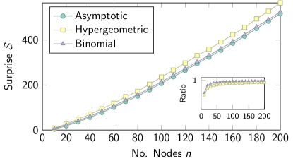
Figure 3: (Color online) Approximation of surprise. The asymptotic formulation of surprise, using the KL divergence, approximates well both the binomial and the hypergeometric surprise. The inset shows the approximation ratio $\mathcal{S}_{\text{asym}}/\mathcal{S}_{\text{hyper}}$ and $\mathcal{S}_{\text{asym}}/\mathcal{S}_{\text{binom}}$, both going to $1$ for large graphs.

To demonstrate the limitations on surprise and (ER) modularity we create some test networks with a planted partition. We generate networks with average degree $\langle k\rangle=10$ and set $\mu=0.1$. In the first test, we create networks with fixed community sizes $n_{c}=10$ and vary the number of communities $r$. In the second test, we have fixed the number of communities to $2$ but vary the community size $n_{c}$ from $10$ to $500$. We consider whether the planted partition remains optimal by analyzing the quality of the planted partition $\mathcal{S}_{\text{plt}}$ (or $\mathcal{Q}_{\text{plt}}$ for modularity) and the partition found through optimization $\mathcal{S}$ (or $\mathcal{Q}$ for modularity). Whenever $\mathcal{S}_{\text{plt}}<\mathcal{S}$ we thus know that the planted partition remains no longer optimal. The results shown in Fig. 2 clearly confirm our theoretical analysis. In the case where $r\to\infty$ with fixed $n_{c}$, surprise does well, whereas (ER) modularity suffers from the resolution limit. In the case that $r$ is fixed to $r=2$, but $n_{c}\to\infty$, surprise does less well, as it tends to find subgraphs within the two large communities. Modularity also has problems identifying the optimal bisection. Indeed, the uncovered partitions do not coincide exactly with the planted partition, even though the modularity value remains rather similar. Such partitions are likely to occur because of the degeneracy of modularity Good, de Montjoye, and Clauset (2010). Nonetheless, our results show that the modularity of the planted partition remains (nearly) optimal, whereas surprise for the planted partition clearly diminishes compared to surprise of the uncovered partitions.

We also tested the various methods more extensively using benchmark graphs with a more realistic community size and degree distribution Lancichinetti, Fortunato, and Radicchi (2008). We set the average degree $\langle k\rangle=20$ while the maximum degree is $50$ and follows a powerlaw degree distribution with exponent $2$. Planted community sizes range from $10$ to $50$ for the “small” communities, and from $20$ to $100$ for “large” communities. The planted community sizes are also distributed according to a powerlaw, but with an exponent of $1$. The parameter $\mu$ again controls the probability of internal links.

In Fig. 4 we show the function values for surprise, significance and ER modularity. This clearly shows that the inequalities hold over the whole range of mixing parameters. At the same time, they show very similar behavior to each other. Although this could indicate a relatively similar performance, we next show this is not the case.

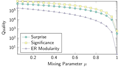
Figure 4: (Color online) Inequalities. In most cases significance is more discriminative than surprise, which is more discriminative than the ER modularity, so that $\mathcal{Z}>\mathcal{S}>\mathcal{Q}_{\text{ER}}$. These inequalities clearly hold over the whole range of the mixing parameter $\mu$ for LFR benchmarks ($n=10^{4}$). For ER modularity we display $2m\mathcal{Q}_{\text{ER}}^{2}$ as used in Eq. (14).

In Fig. 5 we show the benchmark results for the four different methods. Surprise and significance performances are very good, and clearly much better than both modularity models. Notice that, surprise and ER modularity use the same global quantities. However, the use of the KL divergence gives the former a much greater advantage, as expected from Eq. (14).

LFR benchmark graphs have a clearer community structure for larger graphs. The critical mixing parameter at which the inner community density equals the outer community density is roughly $\mu\approx 1-\frac{n_{c}}{n}$, so that with growing $n$ this threshold goes to $1$. Both surprise and significance start to work better for somewhat larger graphs, consistent with the clearer community structure. This is in a sense the opposite of both ER and CM modularity. Their performance is worse for larger graphs, consistent with our earlier analysis of the limitations of community detection.

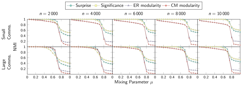
Figure 5: (Color online) Benchmark results. The first row shows results for “small” communities, which range from $10$–$50$, while the second row contains results for “large” communities, ranging from $20$–$100$. The community sizes are powerlaw distributed with exponent $1$. We set the average degree $\langle k\rangle=20$ and the maximum degree is $50$, which follows a powerlaw degree distribution with exponent $2$. Both surprise and significance perform very well, especially for relatively large graphs, where ER and CM modularity fail. This difference is more notable for smaller communities, for which both ER and CM modularity have difficulties. This is in part due to the well-known resolution limit and in line with our earlier analysis.

VI Conclusion

Community detection is an important topic in the field of complex networks, as it can give us a better understanding of real-world networks. Here we analyzed a recent measure known as surprise. We developed an accurate asymptotic approximation, based on the KL divergence which we use to develop a competitive new algorithm. Applying this algorithm to standard benchmarks, we show its great potential. Significance, another quality measure also based on the KL divergence performs similar to surprise.

We showed analytically that surprise is more discriminative than modularity with an ER null model. This is mainly due to the use of the KL divergence to quantify the difference between the empirical partition and the null model. The larger the network and the smaller the communities, the better KL methods perform with respect to modularity. Indeed, whereas modularity suffers from the resolution limit, this problems (nearly) doesn’t affect surprise. On the other hand, surprise tends to find substructure in larger communities, arising from random fluctuations, whereas this problems appears less prominent for modularity. In short, modularity tends to work well in the limit of community sizes $n_{c}\to\infty$ keeping the number of communities $r$ fixed. Surprise on the other hand works well when $r\to\infty$ keeping the community sizes $n_{c}$ fixed. Stated differently, modularity tends to underestimate the number of communities, whereas surprise tends to overestimate the number of communities. The question of which method works well in both limits deserves further study.

The slight differences between surprise and significance stem from two things either the one or the other measure ignores. Significance relies on the fraction of edges that are present within a community. It thus implicitly considers missing edges within communities, because this fraction is relative to the total number of possible edges within that community, which surprise does not. Surprise on the other hand, considers the fraction of total edges that fall within communities. It thus implicitly considers edges that fall between communities, whereas significance does not. Indeed, it should be possible to address these shortcomings by also explicitly examining missing links (for surprise) or links between communities (for significance).

Another shortcoming is that surprise does not depend on the actual distribution of the internal edges among communities. One way to address this issue is to consider edges for all communities separately, by using a multivariate hypergeometric distribution. In that case, we would be interested in the probability to observe $m_{cd}$ edges between communities $c$ and $d$ as

$$\Pr(X_{cd}=m_{cd})=\frac{\displaystyle\prod_{cd}\binom{n_{c}n_{d}}{m_{cd}}}{\displaystyle\binom{M}{m}}.$$ (30)

Again deriving an asymptotic expression, we arrive at

$$\mathcal{S}(\mathcal{V})=m\sum_{cd}q_{cd}\log\frac{q_{cd}}{\langle q_{cd}\rangle}=mD(\mathbf{q}\parallel\langle\mathbf{q}\rangle)$$ (31)

where $q_{cd}=\frac{m_{cd}}{m}$ is the fraction of edges between communities $c$ and $d$ and $\langle q_{cd}\rangle$ the expected value.

Interestingly, the extension of surprise in Eq. (30) is identical to a stochastic blockmodel (using an ER null model) Karrer and Newman (2011); Bickel and Chen (2009). However, Karrer and Newman found that this method did not work satisfyingly Karrer and Newman (2011). This might be because the measure does not focus on communities specifically, but rather on all types of block structures. Hence, there is no reason why a community structure should maximize this likelihood, rather than any other type of block structure. One possible way to address this is to compare our partition to the ideal type we are looking for, rather than maximizing the difference to a random null model. This would be an interesting avenue to consider in future research.

Appendix A Asymptotic surprise

As stated in the main text, $q$ denotes the fraction of internal edges, so that we can write $m_{\text{int}}=qm$. Since $m=p\binom{n}{2}=pM$, we thus have $m_{\text{int}}=qpM$. Similarly, we can write $M_{\text{int}}=\langle q\rangle M$. Hence, we obtain

$$m =pM,$$ (32)

$$m_{\text{int}} =qpM,$$ (33)

$$M_{\text{int}} =\langle q\rangle M.$$ (34)

Notice that all quantities now depend on $M$. We only take into account the dominant term, so to obtain

$$\mathcal{S}(\mathcal{V})\approx-\log\frac{\displaystyle\binom{\langle q\rangle M}{pqM}\binom{(1-\langle q\rangle)M}{p(1-q)M}}{\displaystyle\binom{M}{pM}}$$ (35)

which corresponds to the probability of observing exactly $m_{\text{int}}$ internal links. The binomial coefficient $\binom{M}{pM}$ is independent of the partition, so we ignore it. We use Stirling’s approximation of the binomial coefficient which reads

$${\binom{n}{k}}\approx\left(\frac{n}{k}\right)^{k}.$$ (36)

Hence, for the dominant term, we obtain

$$\mathcal{S}(\mathcal{V}) =-\log\left(\frac{\langle q\rangle M}{pqM}\right)^{pqM}\left(\frac{(1-\langle q\rangle)M}{p(1-q)M}\right)^{p(1-q)M}$$ (37)

$$=-\log p^{-pN}\left(\left(\frac{\langle q\rangle}{q}\right)^{q}\left(\frac{1-\langle q\rangle}{1-q}\right)^{1-q}\right)^{pM}.$$ (38)

The term $p^{-pM}$ is independent of the partition and we ignore it, which yields

$$\mathcal{S}(\mathcal{V})=-pM\left(q\log\frac{\langle q\rangle}{q}+(1-q)\log\frac{1-\langle q\rangle}{1-q}\right).$$ (39)

Using $pM=m$, we can rewrite this to

$$\mathcal{S}(\mathcal{V})=mD(q\parallel\langle q\rangle)$$ (40)

where $D(x\parallel y)$ is the KL divergence Kullback and Leibler (1951)

$$D(x\parallel y)=x\log\frac{x}{y}+(1-x)\log\frac{1-x}{1-y},$$ (41)

which can be interpreted as the distance between the two probability distributions $q$ and $\langle q\rangle$.

Appendix B Significance

We can calculate the approximate difference of moving an edge from one community to another. Assume we move an edge from community $r$ to community $s$. The change in the density will be approximately $p_{r}-\frac{1}{n_{r}^{2}}$ and $p_{s}+\frac{1}{n_{s}^{2}}$ respectively. The corresponding difference in significance will be approximately

$$\mathcal{Z}(\mathcal{V}^{\prime})-\mathcal{Z}(\mathcal{V})= n_{s}^{2}\left(D(p_{s}+\frac{1}{n_{s}^{2}}\parallel p)-D(p_{s}\parallel p)\right)$$

$$+n_{r}^{2}\left(D(p_{r}-\frac{1}{n_{r}^{2}}\parallel p)-D(p_{r}\parallel p)\right)$$ (42)

$$\approx \frac{\partial}{\partial p_{s}}D(p_{s}\parallel p)-\frac{\partial}{\partial p_{r}}D(p_{r}\parallel p)$$ (43)

$$= \log\frac{p_{s}}{1-p_{s}}\frac{1-p_{r}}{p_{r}}=\Delta\mathcal{Z}.$$ (44)

This quantity is particularly straightforward (the logarithmic odds ratio), and if $p_{r}>p_{s}$ the difference will be negative, and if $p_{r}<p_{s}$ this quantity will be positive. Moving edges from a denser community to a less dense community decreases the significance. In other words, making two densities more equal decreases the significance. Repeating these steps, we should expect to find the lowest significance when the communities are of equal density.

Alternatively, by convexity of the Kullback-Leibler divergence, we obtain for significance that

$$\mathcal{Z}(\mathcal{V})\geq\left(\sum_{c}\binom{n_{c}}{2}\right)D\left(\sum_{c}\frac{\binom{n_{c}}{2}}{\sum_{c}\binom{n_{c}}{2}}p_{c}\parallel p\right).$$ (45)

Realizing that $m_{c}=p_{c}\binom{n_{c}}{2}$, we see that

$$\sum_{c}\frac{\binom{n_{c}}{2}}{\sum_{c}\binom{n_{c}}{2}}p_{c}=\frac{m_{\text{int}}}{M_{\text{int}}}=p\frac{q}{\langle q\rangle}.$$ (46)

Notice that this can be interpreted as an average internal density $\langle p_{c}\rangle$ as stated in the main text. Using this we arrive at

$$\mathcal{Z}(\mathcal{V})\geq M_{\text{int}}D\left(p\frac{q}{\langle q\rangle}\parallel p\right).$$ (47)

Hence, the significance of a partition with different community densities $p_{c}$ is generally larger than a partition where all communities have the same average density $p_{c}=\frac{m_{\text{int}}}{M_{\text{int}}}$. Notice that $p\frac{q}{\langle q\rangle}$ should be bounded by $1$ so that $q>\langle q\rangle>p\langle q\rangle$ in general.

This points to a bound such that $\mathcal{Z}(\mathcal{V})\geq\mathcal{S}(\mathcal{V})$ when $\langle q\rangle<p$ in the following way. Define $\lambda=\frac{\langle q\rangle}{p}$ so that $\lambda<1$ if $\langle q\rangle<p$. Again applying convexity, we obtain

$$\mathcal{Z}(\mathcal{V}) \geq M_{\text{int}}D(\frac{pq}{\langle q\rangle}\parallel p)$$ (48)

$$=\frac{M_{\text{int}}}{\lambda}\left(\lambda D(\frac{pq}{\langle q\rangle}\parallel p)+(1-\lambda)D(0\parallel 0)\right)$$ (49)

$$\geq\frac{M_{\text{int}}}{\lambda}D(\lambda\frac{pq}{\langle q\rangle}\parallel\lambda p)$$ (50)

$$=m_{\text{int}}D(q\parallel\langle q\rangle)=\mathcal{S}(\mathcal{V}).$$ (51)

If there are fewer communities (i.e. if $p>\langle q\rangle$) the relationship is not entirely clear, but there are cases for which surprise may be larger than significance. For example, if we assume an equi-sized equi-dense partition with $r$ communities, then $q=\frac{p_{c}\langle q\rangle}{p}$ and $\langle q\rangle=\frac{1}{r}$, and the difference can be written as

$$\mathcal{S}(\mathcal{V})-\mathcal{Z}(\mathcal{V})=m(1-q)\log\frac{1-q}{1-\langle q\rangle}\\ -M_{\text{int}}(1-p_{c})\log\frac{1-p_{c}}{1-p}.$$ (52)

Indeed if $\langle q\rangle>p$ then $\mathcal{S}(\mathcal{V})>\mathcal{Z}(\mathcal{V})$ for equi-sized equi-dense partitions. Keep in mind though that an equi-sized equally dense partition will have a lower significance in general, so that this does not hold for $\langle q\rangle>p$ in general.

References

- Albert and Barabási (2002) R. Albert and A.-L. Barabási, Rev. Mod. Phys. 74, 47 (2002).
- Dorogovtsev (2010) S. Dorogovtsev, Lectures on complex networks (Oxford University Press, 2010).
- Newman (2010) M. Newman, Networks: An Introduction (Oxford University Press, USA, 2010).
- Barabási and Albert (1999) A.-L. Barabási and R. Albert, Science 286, 509 (1999).
- Watts and Strogatz (1998) D. J. Watts and S. H. Strogatz, Nature 393, 440 (1998).
- Fortunato (2010) S. Fortunato, Physics Reports 486, 75 (2010).
- Girvan and Newman (2002) M. Girvan and M. E. J. Newman, Proceedings of the National Academy of Sciences of the United States of America 99, 7821 (2002).
- Gleiser and Danon (2003) P. M. Gleiser and L. Danon, Adv. Complex Syst. 06, 565 (2003).
- Palla and Dere (2005) G. Palla and I. Dere, Nature 435 (2005), 10.1038/nature03607.
- Guimerà et al. (2005) R. Guimerà, S. Mossa, A. Turtschi, and L. A. N. Amaral, Proceedings of the National Academy of Sciences of the United States of America 102, 7794 (2005).
- Olesen et al. (2007) J. M. Olesen, J. Bascompte, Y. L. Dupont, and P. Jordano, Proc. Natl. Acad. Sci. U. S. A. 104, 19891 (2007).
- Lupu and Traag (2013) Y. Lupu and V. Traag, Journal of Conflict Resolution 57, 1011 (2013).
- Danon, D, and Duch (2005) L. Danon, A. D, and J. Duch, Journal of Statistical Mechanics: Theory and Experiment P09008 (2005).
- Lancichinetti et al. (2011) A. Lancichinetti, F. Radicchi, J. J. Ramasco, and S. Fortunato, PLoS ONE 6, e18961 (2011).
- Aldecoa and Marín (2013a) R. Aldecoa and I. Marín, Scientific reports 3, 1060 (2013a).
- Newman and Girvan (2004) M. E. J. Newman and M. Girvan, Physical Review E 69, 026113 (2004).
- Reichardt and Bornholdt (2006) J. Reichardt and S. Bornholdt, Physical Review E 74, 016110+ (2006).
- Ronhovde and Nussinov (2010) P. Ronhovde and Z. Nussinov, Physical Review E 81, 046114 (2010).
- Lancichinetti and Fortunato (2009) A. Lancichinetti and S. Fortunato, Physical Review E 80, 056117 (2009).
- Good, de Montjoye, and Clauset (2010) B. H. Good, Y.-A. de Montjoye, and A. Clauset, Physical Review E 81, 046106 (2010).
- Aldecoa and Marín (2013b) R. Aldecoa and I. Marín, Sci. Rep. 3, 2216 (2013b).
- Traag, Krings, and Van Dooren (2013) V. A. Traag, G. Krings, and P. Van Dooren, Scientific Reports 3, 2930 (2013).
- Fortunato and Barthélemy (2007) S. Fortunato and M. Barthélemy, Proceedings of the National Academy of Sciences 104, 36 (2007).
- Kumpula et al. (2007) J. M. Kumpula, J. Saramäki, K. Kaski, and J. Kertész, The European Physical Journal B 56, 41 (2007).
- Lancichinetti and Fortunato (2011) A. Lancichinetti and S. Fortunato, Physical Review E 84, 066122 (2011).
- Bagrow (2012) J. P. Bagrow, Physical Review E 85, 066118 (2012).
- Xiang and Hu (2012) J. Xiang and K. Hu, Physica A: Statistical Mechanics and its Applications 391, 4995 (2012).
- Kehagias (2012) A. Kehagias, (2012).
- Traag, Van Dooren, and Nesterov (2011) V. A. Traag, P. Van Dooren, and Y. Nesterov, Physical Review E Phys. Rev. E, Stat. Nonlinear Soft Matter Phys. (USA), 84, 016114 (2011).
- Aldecoa and Marín (2011) R. Aldecoa and I. Marín, PLoS ONE 6, e24195 (2011).
- Kullback and Leibler (1951) S. Kullback and R. A. Leibler, Ann. Math. Stat. 22, 79 (1951).
- Decelle et al. (2011) A. Decelle, F. Krzakala, C. Moore, and Z. Lenka, Physical Review Letters 107, 065701 (2011).
- Arnau, Mars, and Marín (2005) V. Arnau, S. Mars, and I. Marín, Bioinformatics 21, 364 (2005).
- Aldecoa and Marín (2014) R. Aldecoa and I. Marín, Bioinformatics 30, 1041 (2014).
- Blondel et al. (2008) V. D. Blondel, J.-L. Guillaume, R. Lambiotte, and E. Lefebvre, Journal of Statistical Mechanics: Theory and Experiment P10008 (2008).
- Porter, Onnela, and Mucha (2009) M. A. Porter, J.-p. Onnela, and P. J. Mucha, Notices of the AMS 56, 1082 (2009).
- Molloy and Reed (1995) M. Molloy and B. Reed, Random structures & algorithms 6, 161 (1995).
- Krings and Blondel (2011) G. Krings and V. D. Blondel, (2011).
- Traag (2014) V. A. Traag, Algorithms and Dynamical Models for Communities and Reputation in Social Networks, Springer Theses (Springer, Heidelberg, 2014).
- Schaub et al. (2012) M. T. Schaub, J.-C. Delvenne, S. N. Yaliraki, and M. Barahona, PloS one 7, e32210 (2012).
- Radicchi (2014) F. Radicchi, EPL (Europhysics Letters) 106, 38001 (2014).
- Nadakuditi and Newman (2012) R. R. Nadakuditi and M. E. J. Newman, Physical Review Letters 108, 188701 (2012).
- Radicchi (2013) F. Radicchi, Physical Review E 88, 010801 (2013), arXiv:1306.1102 [cond-mat, physics:physics].
- Lancichinetti, Fortunato, and Radicchi (2008) A. Lancichinetti, S. Fortunato, and F. Radicchi, Phys. Rev. E - Stat. Nonlinear, Soft Matter Phys. 78 (2008).
- Karrer and Newman (2011) B. Karrer and M. E. J. Newman, Physical Review E 83, 016107 (2011).
- Bickel and Chen (2009) P. J. Bickel and A. Chen, Proceedings of the National Academy of Sciences 106, 21068 (2009).