Optimal configurations of lines and a statistical application

Abstract.

Motivated by the construction of confidence intervals in statistics, we study optimal configurations of $2^{d}-1$ lines in real projective space $\mathbb{R}\mathbb{P}^{d-1}$. For small $d$, we determine line sets that numerically minimize a wide variety of potential functions among all configurations of $2^{d}-1$ lines through the origin. Numerical experiments verify that our findings enable to assess efficiently the tightness of a bound arising from the statistical literature.

1. Introduction

Motivated by a question arising from statistics related to the construction of uniformly valid post-selection confidence intervals [3, 5], whose details we present below, we aim at computing $2^{d}-1$ evenly-spaced lines through the origin in $\mathbb{R}^{d}$. The terminology “evenly-spaced” is loose and, indeed, there are several mathematical formulations that make sense but often lead to different types of line sets. Usually, one considers a potential energy with a “repulsive” pairwise interaction kernel, and a line set may be called evenly-spaced if it is optimal with respect to this energy. However, note that optimal line sets may differ among different potential energies. For very particular choices of the number of lines with respect to the ambient dimension $d$, see [8], optimal lines coincide for a large class of monotonic pairwise interaction kernels considered in [7] and are therefore called universally optimal. However, universal optimality is a rare event in the sense that only very few configurations can exist and even fewer are actually proven to be universally optimal. Indeed, in general it is extremely difficult to prove that a certain configuration is universally optimal, cf. [7, 8, 9].

In the present paper, we consider configurations of $2^{d}-1$ lines in $\mathbb{R}^{d}$ for $d=2,\ldots,6$ that minimize (not necessarily simultaneously) three types of potential energies associated to the distance-, the Riesz-$1$-, and the log-kernels. Additionally, we compare these minimizers to the corresponding best packings of lines found in [10], which can be seen as limiting cases of potential energy minimizers. In dimension $d=2,3$, all the three minimizing configurations of $3$ and $7$ lines, respectively, are known to coincide with the corresponding best packings of lines, by virtue of their universal optimality [8]. Unfortunately, for $d=4,5$ our numerical experiments suggest that there are no universally optimal line sets. Surprisingly, for $d=6$ there seems to exist a universally optimal configuration of $63$ lines, which we identified as the best packing configuration provided in [10]. However, this particular configuration, which can be composed by the $36$ lines going through the vertices and the $27$ lines going through the centers of the $5$-faces of the $1_{22}$ polytope (also called the $E_{6}$ polytope), cannot be proven to be universally optimal with the so-call sharpness condition introduced in [7], so that we state its universal optimality as a conjecture.

Let us now present the statistical application. In the context of the construction of valid post-model-selection confidence intervals, [3, 5] have proposed new confidence intervals that are derived from evaluating a special statistical potential function of at most $2^{d}-1$ many lines in $\mathbb{R}^{d}$. It is desirable to find the maximum of this function, when the lines are subject to certain restrictions [3, 5]. Due to the inherent complexity of these restrictions and of the statistical potential itself, direct optimization approaches seem hopeless. However, a standard upper bound is available for this maximum [5], derived by two consecutive inequalities, cf. (3) and (4) in Section 2. It is known that the second inequality is an equality for $d=2$ [3, Lemma A.4] and that it is tight as $d\to\infty$ [5]. In the present paper, we shall complete this picture for other small values of $d$ by simply evaluating the statistical potential at sets of $2^{d}-1$ evenly-spaced lines. These evaluations are very close to the upper bound, which demonstrate the tightness of the second inequality. Moreover, for universally optimal line sets, the gap is significantly smaller, which underlines that special property.

The outline is as follows. In Section 2, we fix notation and present the statistical potential that motivates us to search for $2^{d}-1$ evenly-spaced lines in $\mathbb{R}^{d}$. The potential energies in projective space are introduced in Section 3, where we also provide the definitions of the distance-, the Riesz-$s$-, and the log-energy [17] as well as the notion of universal optimal configurations of lines [7]. For each dimension $d=2,\dots,6$ we provide in Section 4 one of the numerically found minimizers of the distance-, the Riesz-$1$-, or the log-energy. Section 5 is dedicated to the statistical application, in which we compare the performance of the evenly-spaced lines with a naive Monte Carlo optimization of the statistical potential.

2. Notation and motivation

Let $\mathbb{S}^{d-1}$ denote the unit sphere and $\mathbb{R}\mathbb{P}^{d-1}$ the projective space (the set of lines through the origin) of $\mathbb{R}^{d}$. Any $u\in\mathbb{S}^{d-1}$ defines a line $\ell\in\mathbb{R}\mathbb{P}^{d-1}$ by $\ell=u\mathbb{R}$, and its antipodal counterpart $-u$ yields the same line. Throughout the entire manuscript, we shall fix $N:=N(d):=2^{d}-1$. The set of all sets of at most $N$ lines is denoted by $\mathcal{D}_{\leq N}:=\mathcal{D}_{\leq N}(d):=\{L\subset\mathbb{R}\mathbb{P}^{d-1},\,\#L\leq N\}$ and the set of all sets of exactly $N$ lines is denoted by $\mathcal{D}_{N}:=\{L\subset\mathbb{R}\mathbb{P}^{d-1},\,\#L=N\}$.

In order to construct valid confidence intervals in statistical model selection, the authors in [3, 5] consider a function

$$f_{d,r,\alpha}:\mathcal{D}_{\leq N}\rightarrow\mathbb{R}_{+},$$

where $\alpha\in(0,1)$ and $r\in\mathbb{N}^{*}$ are fixed parameters. The value of $f_{d,r,\alpha}(L)$, for $L\in D_{\leq N}$, is defined as the unique $K>0$ such that

(1) $$\mathbb{E}_{V}\Big{(}F_{d,r}\big{(}\frac{K^{2}}{d\cdot\!\!\max\limits_{u\mathbb{R}=\ell\in L}\langle u,V\rangle^{2}}\big{)}\Big{)}=1-\alpha,$$

where $F_{d,r}$ is the cumulative distribution function of the F-distribution with parameters $d$ and $r$, and $V$ is a uniformly distributed random vector on $\mathbb{S}^{d-1}$. In the statistical context, for fixed values of $\alpha$ and $r$, it is desirable to find the maximum of $f_{d,r,\alpha}$ on a certain subset $\tilde{\mathcal{D}}\subset\mathcal{D}_{\leq N}$, cf. [3, 5], i.e., one aims to determine

(2) $$\sup_{L\in\widetilde{\mathcal{D}}}f_{d,r,\alpha}(L),$$

where each set of lines in $\tilde{\mathcal{D}}$ is derived from some statistical data set but where $\tilde{D}$ depends only on $d$, cf. [5, Equations (5.2) and (5.3) and Section 4.10] and [3, Equation (6)]. Note that [3] and [5] yield two different subsets $\tilde{\mathcal{D}}$, but this difference is of no consequence in the sequel. Considering the supremum (2) is beneficial because this supremum is data-independent and can be tabulated, for fixed $r$ and $\alpha$, once and for all.

Exactly determining (2) is difficult if not computationally infeasible since the set $\tilde{\mathcal{D}}$ is defined in [3] or [5] in an intricate manner, that has so far made it impossible to determine (2) theoretically. Moreover, the values $f_{d,r,\alpha}(L)$ can usually only be approximated by Monte Carlo methods, as in Algorithm 1, which we write only for the case of sets of $N$ lines, for concision. Note, that Algorithm 1 is also used in [3].

In [3, 5], an upper bound $\bar{K}(d,r,\alpha)$ has been proposed for (2) that can easily be determined numerically, and we refer to Proposition 2.3 and Algorithm 4.3 in [3] for its definition and computation. This bound satisfies the following sequential inequalities:

(3) $$\sup_{L\in\widetilde{\mathcal{D}}}f_{d,r,\alpha}(L) \leq\sup_{L\in\mathcal{D}_{N}}f_{d,r,\alpha}(L)$$

(4) $$\leq\bar{K}(d,r,\alpha),$$

where (3) is due to $\tilde{\mathcal{D}}\subset\mathcal{D}_{\leq N}$ and to the fact that $K$ in (1) is increased if additional lines are added, so that $\sup_{L\in\mathcal{D}_{\leq N}}f_{d,r,\alpha}(L)=\sup_{L\in\mathcal{D}_{N}}f_{d,r,\alpha}(L)$. The inequality (4) is derived from a union bound, cf. Equation (A.17) in [5].

As noted in [5] and [3, Remark 2.10], the inequality (4) is tight for large values of $d$, i.e.,

(5) $$\frac{\sup_{L\in\mathcal{D}_{N}}f_{d,r,\alpha}(L)}{\bar{K}(d,r,\alpha)}\rightarrow 1,$$

when $d$ tends to infinity, cf. [5, proof of Theorem 6.3]. For $d=2$, we even have $\sup_{L\in\mathcal{D}_{N}}f_{d,r,\alpha}(L)=\bar{K}(d,r,\alpha)$, see [3, Lemma A.4].

In the present paper, we shall assess whether the upper bound $\bar{K}(d,r,\alpha)$ in (4) for $\sup_{L\in\mathcal{D}_{N}}f_{d,r,\alpha}(L)$ is also tight for small values of $d$.

To evaluate the quality of the inequality (4), we must approximate

(6) $$\sup_{L\in\mathcal{D}_{N}}f_{d,r,\alpha}(L)$$

to determine its difference to $\bar{K}(d,r,\alpha)$. However, exactly computing (6) is also difficult, if not numerically infeasible, and we shall rather aim to derive good lower bounds. In fact, we shall verify that evaluating $f_{d,r,\alpha}$ on one or few candidates of evenly-spaced lines $L=\{\ell_{1},\ldots,\ell_{N}\}\subset\mathbb{R}\mathbb{P}^{d-1}$ yields better lower bounds on (6) than several Monte Carlo attempts. Our numerical results on this issue are presented in Section 5.

Remark 2.1.

The quantity $K_{2}$ in [3] corresponds to (2) where the supremum holds over a certain subset $\bar{\mathcal{D}}$ that depends on other quantities beside $d$ (it is data dependent). In the case of $K_{2}$, there exists another upper-bound $K_{3}$ in [3], which is smaller than $\bar{K}(d,r,\alpha)$, incomparable with $\sup_{L\in\mathcal{D}_{N}}f_{d,r,\alpha}(L)$ and convenient to compute. Nevertheless, the context of this paper, where the subset $\tilde{\mathcal{D}}$ is data independent, is unrelated to $K_{3}$, so that $\bar{K}(d,r,\alpha)$ is the only available upper-bound for (2).

3. Potential functions in real projective space

We shall now consider families of potential energies whose minimization can provide us with rather evenly-spaced lines. We recall that the chordal distance $d_{c}$ between two lines $\ell_{i},\ell_{j}\in\mathbb{R}\mathbb{P}^{d-1}$ is given by

(7) $$d^{2}_{c}(\ell_{i},\ell_{j})=\frac{1}{2}\|u_{i}u_{i}^{\top}-u_{j}u_{j}^{\top}\|^{2},$$

where $\ell_{i}=u_{i}\mathbb{R}$ and $\ell_{j}=u_{j}\mathbb{R}$ with $u_{i},u_{j}\in\mathbb{S}^{d-1}$. Let $f:(0,1]\rightarrow\mathbb{R}$ be a decreasing continuous function. For fixed $N$ and $d$, we aim to minimize the potential energy

(8) $$\begin{split}\mathcal{P}_{f}:\mathcal{D}_{N}&\rightarrow\mathbb{R}\\ \{\ell_{1},\ldots,\ell_{N}\}&\mapsto\sum_{i\neq j}f(d^{2}_{c}(\ell_{i},\ell_{j})),\end{split}$$

i.e., we aim to find $\hat{L}\in\mathcal{D}_{N}$ such that

$$\mathcal{P}_{f}(\hat{L})\leq\mathcal{P}_{f}(L),\quad\text{ for all }L\in\mathcal{D}_{N}.$$

We shall explicitly consider three types of pairwise interaction kernels,

1. the distance-energy,

   $$f_{1}(t)=-\sqrt{t},$$

2. the Riesz-$s$-energy,

   $$f_{2}(t)=t^{-s/2},\quad\text{for $s>0$},$$

3. the log-energy,

   $$f_{3}(t)=-\log(t),$$

and we refer to [8, 9, 14, 15, 16, 17, 18] and references therein, for investigations on their minimizers and asymptotic results when $N$ tends to infinity.

We call a function $f:(0,1]\rightarrow\mathbb{R}$ completely monotonic if it is infinitely often differentiable and $(-1)^{k}f^{(k)}\geq 0$, for $k=1,2,\ldots$. Note that the above $f_{1},f_{2},f_{3}$ satisfy this property. The following definition is borrowed from [7].

Definition 3.1.

We call $\hat{L}\in\mathcal{D}_{N}$ universally optimal if it minimizes $\mathcal{P}_{f}$ among $\mathcal{D}_{N}$, for all completely monotonic functions $f$.

Additionally, it seems natural to consider configurations solving the packing problem of $N$ lines in $\mathbb{R}\mathbb{P}^{d-1}$, i.e., sets of lines which maximize the minimal chordal distance, i.e., find $\{\hat{\ell}_{1},\ldots,\hat{\ell}_{N}\}\in\mathcal{D}_{N}$ such that

$$\min_{i\neq j}d_{c}(\hat{\ell}_{i},\hat{\ell}_{j})\geq\min_{i\neq j}d_{c}(\ell_{i},\ell_{j}),\quad\text{ for all }\{\ell_{1},\ldots,\ell_{N}\}\in\mathcal{D}_{N},$$

cf. [10]. Note that the packing problem corresponds to the limit case of the Riesz-$s$-potential when $s$ tends to infinity. In particular, if the set $\{\hat{\ell}_{1},\ldots,\hat{\ell}_{N}\}\in\mathcal{D}_{N}$ is universally optimal, it also solves the packing problem.

For packings in Grassmannians beyond the projective space, we refer to [10, 6], see also [2].

4. $2^{d}-1$ evenly-spaced lines in small dimensions

Recall that we are interested in minimizers of the distance-, Riesz-$1$-, and the log-energy for $N=2^{d}-1$ with $d=2,\ldots,6$. Note, that for each potential energy there exist lots of local minimizers and, unless all such minimizers have been determined, there is no general statement that one has already found a global minimizer.

Here, we repeatedly apply a local optimization procedure initialized by randomly chosen starting points (in our case the nonlinear CG method described in [12, 13]), and we are convinced that the line configurations we present are actually minimizers of the corresponding energies.

In general the minimizers of each of the three potential energies are different. However, since the different configurations perform rather equally well for the statistical potential we will provide for each dimension only one selected minimizer explicitly.

4.1. Universally optimal lines in $\mathbb{R}^{2}$

It is known that three equiangular lines in $\mathbb{R}^{2}$ are universally optimal, cf. [7], hence all minimizers coincide with that best packing configuration. For instance, such lines $\{\ell_{k}\}_{k=1}^{3}$ are given by the vectors $u_{k}=(\cos(\tfrac{2}{3}k\pi),\sin(\tfrac{2}{3}k\pi))^{\top}$, with $\ell_{k}=u_{k}\mathbb{R}$, for $k=1,2,3$. Note that this configuration is highly symmetric and generated by a single orbit of its symmetry group $D_{3}$, which is the dihedral group of order $|D_{3}|=6$.

Remark 4.1.

It is known that those $\{\ell_{1},\ell_{2},\ell_{3}\}$ maximize $f_{2,r,\alpha}$ and, as mentioned before, the maximum indeed coincides with $\bar{K}(d,r,\alpha)$, cf. [3, Lemma A.4].

4.2. Universally optimal lines in $\mathbb{R}^{3}$

It has been proven recently that there exist $7$ lines that are universally optimal in $\mathbb{R}\mathbb{P}^{2}$, see [9], hence all minimizers coincide with that best packing configuration. In such a configuration, $4$ lines are going through the vertices and 3 through the centers of the faces of a cube centered at the origin, see Figure 1. If the cube’s edges are aligned with the coordinate axis, then the lines $\{\ell_{k}=u_{k}\mathbb{R}\}_{k=1}^{7}$ are given by the vectors

$$u_{1} =(1,1,1)^{\top},\quad u_{2}=(1,-1,1)^{\top},\quad u_{3}=(-1,1,1)^{\top},\quad u_{4}=(-1,-1,1)^{\top}$$

$$u_{5} =(1,0,0)^{\top},\quad u_{6}=(0,1,0)^{\top},\quad u_{7}=(0,0,1)^{\top}.$$

Note that this configuration is also highly symmetric and is generated by only $2$ orbits of its symmetry group $O_{h}$, which is the full octahedral group of order $|O_{h}|=48$.

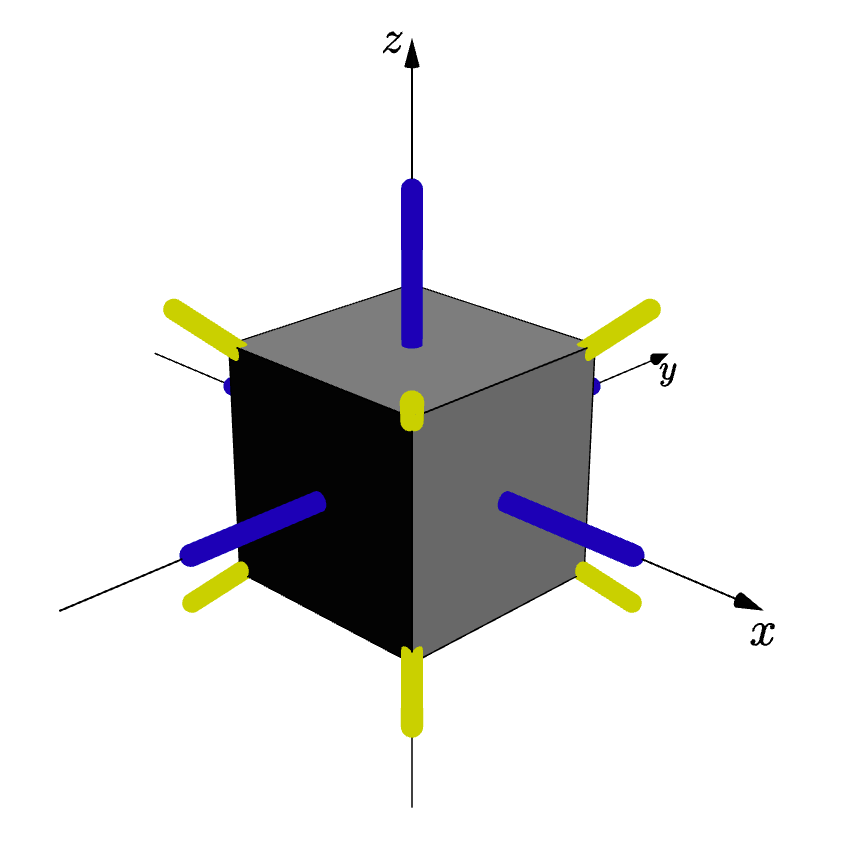
Figure 1. $7$ universally optimal lines in $\mathbb{R}^{3}$.

4.3. Optimal lines in $\mathbb{R}^{4}$

Our numerical computations provide us with strong evidence that there are no universally optimal configurations of $15$ lines in $\mathbb{R}\mathbb{P}^{4}$. We found a very symmetric configuration $L=\{\ell_{k}\}_{k=1}^{15}$, which seems to minimize the log-energy and the Riesz-$1$-energy simultaneously. It is more symmetric than our numerical minimizer of the distance-energy in the sense that it is composed by fewer group orbits. Moreover one can simply check that it is a stationary point of any Riesz-$s$-energy, $s>0$. However, it does not solve the best packing problem (the limiting case $s\to\infty$), as it has a slightly smaller minimal distance than the configuration found in [10].

The symmetry group $\mathcal{G}$ of $L$ as a subgroup of the orthogonal matrices $O(4)\subset\mathbb{R}^{4\times 4}$ acts naturally by left multiplication on $\mathbb{R}\mathbb{P}^{3}$. The group has order $|\mathcal{G}|=144$ and is generated by the following matrices

$$G_{1} =-\begin{pmatrix}1&0&0&0\\ 0&1&0&0\\ 0&0&1&0\\ 0&0&0&1\end{pmatrix},\quad G_{2}=\begin{pmatrix}0&0&0&1\\ 0&0&1&0\\ 0&1&0&0\\ 1&0&0&0\end{pmatrix},\quad G_{3}=\begin{pmatrix}-1&0&0&0\\ 0&1&0&0\\ 0&0&1&0\\ 0&0&0&1\end{pmatrix},$$

$$G_{4} =\frac{1}{2}\begin{pmatrix}-1&-\sqrt{3}&0&0\\ \sqrt{3}&-1&0&0\\ 0&0&1&0\\ 0&0&0&1\end{pmatrix},\quad G_{5}=\frac{1}{2}\begin{pmatrix}-1&-\sqrt{3}&0&0\\ \sqrt{3}&-1&0&0\\ 0&0&-1&-\sqrt{3}\\ 0&0&\sqrt{3}&-1\end{pmatrix}.$$

The $15$ lines $L=L_{1}\cup L_{2}$ are composed by the two orbits

$$L_{1} =\{u\mathbb{R}\;|\;u=G\cdot(1,0,0,0)^{\top},G\in\mathcal{G}\},$$

$$L_{2} =\{u\mathbb{R}\;|\;u=G\cdot(0,1,1,0)^{\top},G\in\mathcal{G}\}$$

of cardinality $6$ and $9$, respectively. See Figure 2, for a visualization.

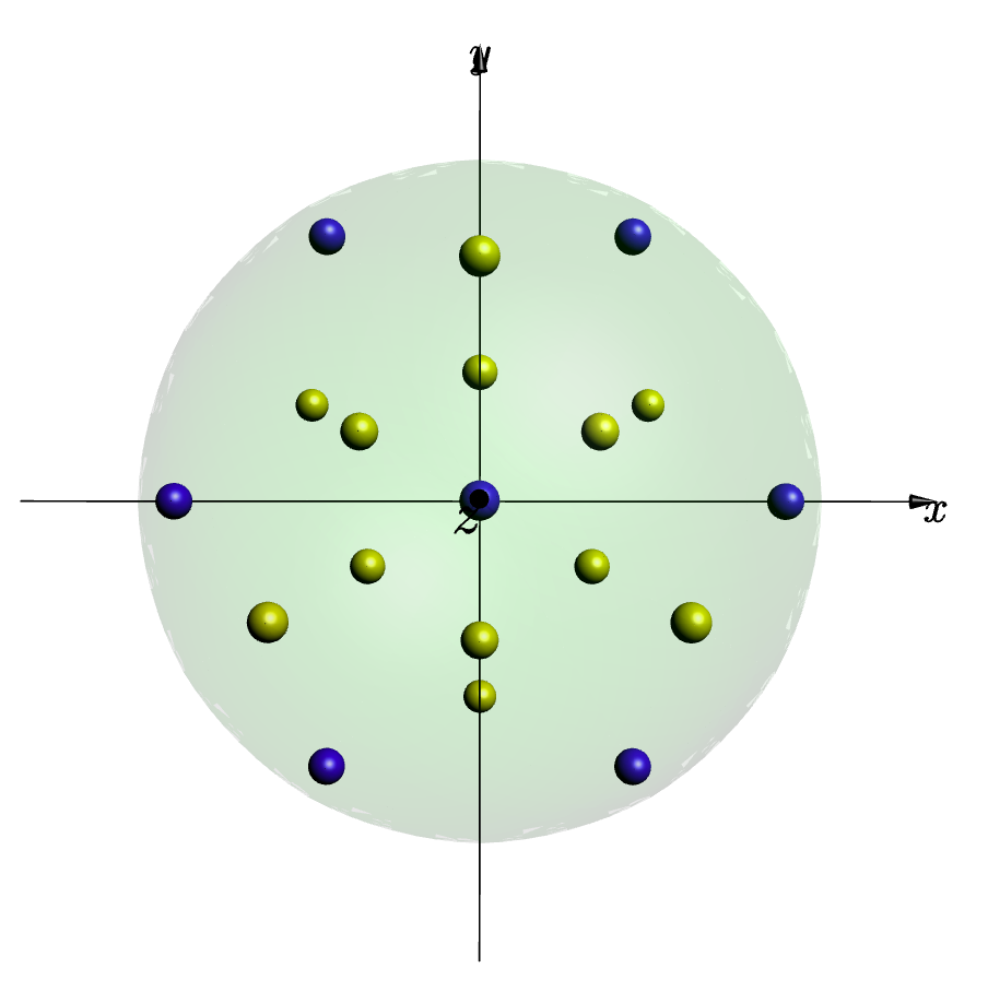
Figure 2. $15$ lines in $\mathbb{R}^{4}$ visualized in the unit ball in $\mathbb{R}^{3}$. Blue points correspond to orbit $L_{1}$, yellow correspond to $L_{2}$. For visualization, we consider the intersection of lines in $\mathbb{R}^{4}$ with the upper hemisphere of the unit sphere. Hence, lines become points. Now, we apply the stereographic projection to map the upper hemisphere in $\mathbb{R}^{4}$ into the full ball in $\mathbb{R}^{3}$, which we can plot. In general, a line in $\mathbb{R}^{4}$ reduces to a single point in the ball but lines that intersect the equator have two intersection points and we plot both.

4.4. Optimal lines in $\mathbb{R}^{5}$

We numerically derived different minimizers for each of the three potential energies. They all have a nontrivial symmetry group, and we want to provide the most symmetric configuration of lines, which is found for the Riesz-$1$-energy. In that case the $31$ lines $L=\{\ell_{k}\}_{k=1}^{31}$ are composed by $8$ orbits of its symmetry group. More precisely, the symmetry group $\mathcal{G}$ has order $|\mathcal{G}|=12$ and is generated by the following three matrices

$$G_{1} =-\begin{pmatrix}1&0&0&0&0\\ 0&1&0&0&0\\ 0&0&1&0&0\\ 0&0&0&1&0\\ 0&0&0&0&1\end{pmatrix},\quad G_{2}=\begin{pmatrix}1&0&0&0&0\\ 0&-1&0&0&0\\ 0&0&1&0&0\\ 0&0&0&-1&0\\ 0&0&0&0&1\end{pmatrix},$$

$$G_{3} =\frac{1}{2}\begin{pmatrix}2&0&0&0&0\\ 0&-1&-\sqrt{3}&0&0\\ 0&\sqrt{3}&-1&0&0\\ 0&0&0&-1&-\sqrt{3}\\ 0&0&0&\sqrt{3}&-1\end{pmatrix}.$$

The 31 lines $L=\bigcup_{i=1}^{8}L_{i}$ are then given by the eight orbits

$$L_{1} =\{u\mathbb{R}\;|\;u=G\cdot(1,0,0,0,0)^{\top},G\in\mathcal{G}\},$$

$$L_{2} =\{u\mathbb{R}\;|\;u=G\cdot(0,1,0,0,0)^{\top},G\in\mathcal{G}\},$$

$$L_{3} =\{u\mathbb{R}\;|\;u=G\cdot(0,a_{1},0,-\sqrt{1-a_{1}^{2}},0)^{\top},G\in\mathcal{G}\},$$

$$L_{4} =\{u\mathbb{R}\;|\;u=G\cdot(b_{1},0,b_{2},0,\sqrt{1-b_{1}^{2}-b_{2}^{2}})^{\top},G\in\mathcal{G}\},$$

$$L_{5} =\{u\mathbb{R}\;|\;u=G\cdot(c_{1},0,-c_{2},0,-\sqrt{1-c_{1}^{2}-c_{2}^{2}})^{\top},G\in\mathcal{G}\},$$

$$L_{6} =\{u\mathbb{R}\;|\;u=G\cdot(d_{1},d_{2},-d_{3},d_{4},\sqrt{1-d_{1}^{2}-d_{2}^{2}-d_{3}^{2}-d_{4}^{2}})^{\top},G\in\mathcal{G}\},$$

$$L_{7} =\{u\mathbb{R}\;|\;u=G\cdot(e_{1},e_{2},e_{3},-e_{4},-\sqrt{1-e_{1}^{2}-e_{2}^{2}-e_{3}^{2}-e_{4}^{2}})^{\top},G\in\mathcal{G}\},$$

$$L_{8} =\{u\mathbb{R}\;|\;u=G\cdot(f_{1},-f_{2},f_{3},f_{4},\sqrt{1-f_{1}^{2}-f_{2}^{2}-f_{3}^{2}-f_{4}^{2}})^{\top},G\in\mathcal{G}\},$$

of size $1$, $3$, $3$, $3$, $3$, $6$, $6$ and $6$, respectively, where the constants can be computed to arbitrary precision by numerical minimization

$$a_{1} =0.1386569...,$$

$$b_{1} =0.6107676...,\quad b_{2}=0.2652528...,$$

$$c_{1} =0.6319241...,\quad c_{2}=0.6489064...,$$

$$d_{1} =0.0959289...,\quad d_{2}=0.6048195...,\quad d_{3}=0.3121361...,\quad d_{4}=0.6715440...,$$

$$e_{1} =0.3556342...,\quad e_{2}=0.0311526...,\quad e_{3}=0.7210732...,\quad e_{4}=0.4584122...,$$

$$f_{1} =0.5842996...,\quad f_{2}=0.4841533...,\quad f_{3}=0.3040229...,\quad f_{4}=0.5287425...\quad.$$

4.5. Optimal lines in $\mathbb{R}^{6}$

Our numerical investigations provide us with evidence that there exists an arrangement of $63$ lines which is universally optimal in $\mathbb{R}\mathbb{P}^{5}$ and thus coincides with the best packing solution presented in [10]. This configuration $L=\{\ell_{k}\}_{k=1}^{63}$ is given by the $36$ lines going through the vertices and the $27$ lines going through the centers of the $5$-faces of the $1_{22}$ polytope, cf. [11], also known as the $E_{6}$ polytope. The symmetry group $\mathcal{G}$ of that polytope has order $|\mathcal{G}|=103680$, which contains the Coxeter group $E_{6}$ as an index $2$ subgroup. The high order of the symmetry group $\mathcal{G}$ shows the remarkably high symmetry of this configuration of lines. Note that the group $\mathcal{G}$ can be generated by $2$ matrices

$$G_{1}=\left(\begin{smallmatrix}-\frac{1}{2}&-\frac{1}{2}&\frac{1}{2}&\frac{1}{2}&0&0\\ -\frac{1}{2}&\frac{1}{2}&0&0&\frac{1}{\sqrt{8}}&\sqrt{\frac{3}{8}}\\ \frac{1}{2}&0&\frac{1}{2}&0&\frac{1}{\sqrt{2}}&0\\ \frac{1}{2}&0&0&\frac{1}{2}&-\frac{1}{\sqrt{8}}&\sqrt{\frac{3}{8}}\\ 0&\frac{1}{\sqrt{8}}&\frac{1}{\sqrt{2}}&-\frac{1}{\sqrt{8}}&-\frac{1}{2}&0\\ 0&\sqrt{\frac{3}{8}}&0&\sqrt{\frac{3}{8}}&0&-\frac{1}{2}\\ \end{smallmatrix}\right),\qquad G_{2}=\begin{pmatrix}1&0&0&0&0&0\\ 0&0&1&0&0\ &0\\ 0&0&0&1&0&0\\ 0&1&0&0&0&0\\ 0&0&0&\ 0&\frac{1}{2}&-\frac{\sqrt{3}}{2}\\ 0&0&0&0&\frac{\sqrt{3}}{2}&\frac{1}{2}\end{pmatrix},$$

so that the $63$ lines $L=L_{1}\cup L_{2}$ are explicitly constructed by the two orbits

$$L_{1} =\{u\mathbb{R}\;|\;u=G\cdot(1,0,0,0,0,0)^{\top},G\in E_{6}\},$$

$$L_{2} =\{u\mathbb{R}\;|\;u=G\cdot(0,0,0,0,\sqrt{3},1)^{\top},G\in E_{6}\}$$

of cardinality $36$ and $27$, respectively. Alternatively, the $63$ lines can be derived from the minimal vectors of the $E_{6}$ lattice and its dual lattice $E_{6}^{*}$, see, for instance, G. Nebe’s and N. Sloane’s website [1].

Note that $L_{1}$ itself satisfies the sharpness condition in the sense of [7] and hence is universally optimal in $\mathbb{R}\mathbb{P}^{5}$. The $63$ lines are not sharp, but we conjecture that they are universally optimal in $\mathbb{R}\mathbb{P}^{5}$. Moreover, the corresponding configurations of $126$ points on the sphere is stationary for any completely monotonic potential function of the squared distance of $126$ points on $\mathbb{S}^{5}$, cf. [4].

5. Applications to the statistical potential

5.1. Two approaches

Now that we have some configurations of $N=2^{d}-1$ evenly-spaced lines in projective space in hand, we can apply them to derive lower bounds on

(9) $$\sup_{\{\ell_{1},\ldots,\ell_{N}\}\in\mathcal{D}_{N}}f_{d,r,\alpha}(\{\ell_{1},\ldots,\ell_{N}\})$$

as was our aim stated in Section 2. We shall compare evaluating $f_{d,r,\alpha}$ at our evenly-spaced lines with a standard Monte Carlo optimization method. Note that $f_{d,r,\alpha}$ cannot be evaluated directly, and we apply Algorithm 1 to do so, which is the same algorithm as [3, Algorithm 4.1], and which is also used by the authors of [5]. To summarize, we shall compare the following two methods:

1. evenly-spaced lines:

   This method simply consists in applying Algorithm 1 with $\{\hat{\ell}_{1},...,\hat{\ell}_{N}\}$ being one of the optimal line sets derived in Section 4.

2. naive Monte Carlo:

   One aims to maximize $f_{d,r,\alpha}$ by Monte Carlo optimization, given in Algorithm 4, which first calls the random line generator in Algorithm 2 and then applies Algorithm 3, which itself repeatedly calls Algorithm 1. This type of Monte Carlo optimization has already been used in [3, Section 5] (in a context unrelated to this paper and the evenly-spaced line method (i)).

Our intention is to check that (i) indeed outperforms (ii). From a computational point of view, (i) has a clear advantage: the set of evenly-spaced lines is obtained numerically once and for all, and can be used for any value of $r$ and $\alpha$. In contrast, one needs to repeat the naive Monte Carlo optimization for each values of $r$ and $\alpha$ under consideration.

Algorithm 1 Evaluation of $f_{d,r,\alpha}$ at $\{\ell_{1},\ldots,\ell_{N}\}$

0:  lines $\{\ell_{1},...,\ell_{N}\}\in\mathcal{D}_{N}$ and some parameter $I\in\mathbb{N}$

0:  $K$ approximating $f_{d,r,\alpha}(\{\ell_{1},...,\ell_{N}\})$.

1:  generate independent uniformly distributed random vectors $\{V_{i}\}_{i=1}^{I}\subset\mathbb{S}^{d-1}$.

2:  for each $i=1,\ldots,I$, calculate $c_{i}=\max_{j=1,\ldots,N}\langle u_{j},V_{i}\rangle^{2}$, where $\ell_{j}=u_{j}\mathbb{R}$.

3:  determine $K$ that solves

(10) $$\frac{1}{I}\sum_{i=1}^{I}F_{d,r}\big{(}\frac{K^{2}}{dc_{i}^{2}}\big{)}=1-\alpha.$$

4:  return  $K$

Algorithm 2 random line generator

0:  $N_{1}$ and a set of probability distributions $\{\nu_{j}\}_{j=1}^{N}$ on $\mathbb{S}^{d-1}$.

0:  $D_{1}\subset\mathcal{D}_{N}$ with $\#D_{1}=N_{1}$.

1:  initialize $D_{1}=\emptyset$

2:  for $i=1,\ldots,N_{1}$ do

3:     for $j=1,\ldots,N$, generate a $\nu_{j}$-distributed random vector $u_{j}\in\mathbb{S}^{d-1}$.

4:     insert the corresponding line set $\{u_{1}\mathbb{R},\ldots,u_{N}\mathbb{R}\}$ into $D_{1}$.

5:  end for

6:  return  $D_{1}$

Algorithm 3 find max

0:  ${D}_{1}$, parameters $N_{2},I_{1},I_{2},I_{3}\in\mathbb{N}$ with $N_{2}\leq\#{D}_{1}$.

0:  approximation of $\max_{{D}_{1}}f_{d,r,\alpha}(\ell_{1},\ldots,\ell_{N})$.

1:  evaluate $f_{d,r,\alpha}$ at all $\{\ell_{1},...,\ell_{N}\}\in{D}_{1}$ with $I=I_{1}$ in Algorithm 1.

2:  keep the $N_{2}$ sets ${D}_{2}\subset{D}_{1}$ that yield the largest evaluations in step 1.

3:  reevaluate $f_{d,r,\alpha}$ at all $\{\ell_{1},...,\ell_{N}\}\in{D}_{2}$ with $I=I_{2}$ in Algorithm 1.

4:  keep the sets $\{\ell^{*}_{1},...,\ell^{*}_{N}\}\in{D}_{2}$ that yields the largest evaluation in step 3.

5:  return  $K$ derived from the reevaluation of $f_{d,r,\alpha}(\{\ell^{*}_{1},...,\ell^{*}_{N}\})$ by Algorithm 1 with $I=I_{3}$.

Algorithm 4 naive Monte Carlo

0:  parameters $N_{1},N_{2},I_{1},I_{2},I_{3}\in\mathbb{N}$ with $N_{2}\leq N_{1}$.

0:  naive approximation of $\sup_{\mathcal{D}_{N}}f_{d,r,\alpha}(\{\ell_{1},\ldots,\ell_{N}\})$.

1:  generate ${D}_{1}\subset\mathcal{D}_{N}$ by calling Algorithm 2 with $N_{1}$ and the uniform distribution on $\mathbb{S}^{d-1}$.

2:  return  $K$ derived from calling Algorithm 3 with ${D}_{1}$, $N_{2},I_{1},I_{2},I_{3}$.

5.2. Numerical experiments

We compare the two methods presented in Section 5.1, for $d=3,4,5,6$. Two values of $r=20,60$ are chosen as representative of practical statistical situations, and $\alpha=0.05$ is chosen since this yields the classical $95\%$ confidence.

In order to further investigate on the approach (i), we shall also consider local searches in proximity to the evenly-spaced lines:

• local evenly-spaced lines:

  We search for the maximum of $f_{d,r,\alpha}$ locally around $\{\hat{\ell}_{1},\ldots,\hat{\ell}_{N}\}$ given as in (i). Indeed, we call Algorithm 2 using $N$ projected Gaussian distributions with isotropic variance $\sigma^{2}=0.1^{2}$ and mean vectors $\{u^{*}_{j}\}_{j=1}^{N}$, respectively. With the resulting set $\mathcal{D}_{1}$, we apply Algorithm 3.

• very local evenly-spaced lines:

  As in (a) but we search even more locally by choosing $\sigma^{2}=0.01^{2}$.

In the numerical experiments, the parameters for (i), (ii), (a), and (b) are chosen by $I=20\,000\,000$, $N_{1}=200\,000$, $N_{2}=20\,000$, $I_{1}=10\,000$, $I_{2}=200\,000$, and $I_{3}=20\,000\,000$. In Figure 3, we report, for each of the configurations of $d$, $r$ ($8$ configurations in total), the ratios $K/\bar{K}(d,r,\alpha)$, where $K$ takes four values obtained by the methods (i), (ii), (a), and (b), and where $\bar{K}(d,r,\alpha)$ is the upper bound in (4). For the methods (i), (a), and (b), for $d=3,6$, a unique set of $2^{d}-1$ lines is under consideration, which minimizes all the potential functions of Section 3. For $d=4,5$ different sets minimize different potentials, but give approximately the same values for $f_{d,r,\alpha}$ (the lines corresponding to the packing problem slightly lag behind the others). Hence, in Figure 3 below, we only report the results for the minimizer of the Riesz-$1$-potential, for concision. The ratios $K/\bar{K}(d,r,\alpha)$ enable us to compare the two methods, (i) and (ii), while those obtained from (a) and (b) address the local optimality of approach (i).

In Figure 3, for the configurations of $d$ and $r$ under consideration, the method (i) using evenly-spaced lines provides a better maximization of $f_{d,r,\alpha}$ over $\mathcal{D}_{N}$ than (ii). Hence, it is beneficial both from a computational and performance point of view.

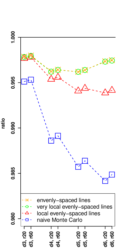
Figure 3. Plot of the ratios $K/\bar{K}(d,r,\alpha)$, where $K$ is obtained from the methods (i), (ii), (a), and (b). We investigate $d=3,4,5,6$, $r=20,60$ and use the minimizers of the Riesz-$1$-potential presented in Section 4 as sets of evenly-spaced lines in methods (i), (a), and (b). The sets of evenly-spaced lines appear to be local maximizers of the statistical potential function, possibly global maximizers for $d=3,6$. They clearly perform better than the naive Monte Carlo maximization (ii).

We also observe in Figure 3 that the values of $K$ obtained from (a) are below those obtained from (b). Furthermore, although not perceptible in the figure, we always have that either $K$ is smaller in (b) than in (i), or the two values cannot be distinguished, because of the very small but positive variance of Algorithm 1. This is numerical indication that the sets of evenly-spaced lines are local maximizers for $f_{d,r,\alpha}$ over $\mathcal{D}_{N}$. At least in the cases $d=3,6$, since we are then dealing with universally optimal lines, it seems plausible that we even obtained the global maximizers.

Note that, in light of Figure 3, $\bar{K}(d,r,\alpha)$ is a tight upper bound in (4) for $d=3,...,6$, with a difference of less than $0.5\%$. This result is of complementary nature with the tightness for large $d$, see (5), derived in [5, proof of Theorem 6.3].

We can conclude that it would not be very beneficial to aim at improving the union bound (4). Instead, one may want to study the inequality (3) more closely. Given the complexity of the sets $\tilde{\mathcal{D}}$ considered in [3] or [5], however, this may require other tools and may turn out to be an extremely challenging task going beyond the scope of the present paper.

We have a smaller window of possible values for (9) in dimensions in which universally optimal lines exist, or are conjectured to exist, with the predefined cardinality $N=2^{d}-1$, see Figure 3 where $d=3,6$ yield higher ratios for (i) than $d=4,5$. In this sense, our statistical application indicates that the concept or property of universal optimality is indeed beneficial.

References

• [1] http://www.math.rwth-aachen.de/$\sim$gabriele.nebe/lattices/.
• [2] C. Bachoc and M. Ehler, Tight $p$-fusion frames, Appl.  Comput.  Harmon.  Anal. 35 (2013), no. 1, 1–15.
• [3] F. Bachoc, H. Leeb, and B. M. Pötscher, Valid confidence intervals for post-model-selection predictors, submitted (2014).
• [4] B. Ballinger, G. Blekherman, H. Cohn, N. Giansiracusa, E. Kelly, and A. Schürmann, Experimental study of energy-minimizing point configurations on spheres, Experiment. Math. 18 (2009), no. 3, 257–283.
• [5] R. Berk, L. Brown, A. Buja, K. Zhang, and L. Zhao, Valid post-selection inference, Ann. Statist. 41 (2013), 802–837.
• [6] A. R. Calderbank, R. H. Hardin, E. M. Rains, P. W. Shor, and N. J. A. Sloane, A group-theoretic framework for the construction of packings in Grassmannian spaces, J. Algebraic Combin. 9 (1997), 129–140.
• [7] H. Cohn and A. Kumar, Universally optimal distribution of points on spheres, J.  Amer.  Math.  Soc. 20 (2007), 99–148.
• [8] H. Cohn, A. Kumar, and G. Minton, Optimal simplices and codes in projective spaces, arXiv:1308.3188 (2013).
• [9] H. Cohn and J. Woo, Three-point bounds for energy minimization, J.  Amer.  Math.  Soc. 25 (2012), no. 4, 929–958.
• [10] J. H. Conway, R. H. Hardin, and N. J. A. Sloane, Packing lines, planes, etc.: packings in Grassmannian space, Experimental Math. 5 (1996), 139–159.
• [11] E. L. Elte, The semiregular polytopes of the hyperspaces, Hoitsema, Groningen, 1912.
• [12] M. Gräf, Efficient algorithms for the computation of optimal quadrature points on riemannian manifolds, Universitätsverlag Chemnitz, 2013.
• [13] M. Gräf, M. Potts, and G. Steidl, Quadrature errors, discrepancies and their relations to halftoning on the torus and the sphere, SIAM J.  Sci.  Comput. (2013).
• [14] D. P. Hardin and E. B. Saff, Minimal Riesz energy point configurations for rectifiable d-dimensional manifolds, Adv.  Math. 193 (2005), no. 1, 174–204.
• [15] S. G. Hoggar, $t$-designs in projective spaces, Europ.  J.  Combinatorics 3 (1982), 233–254.
• [16] A. B. J. Kuijlaars and E. B. Saff, Asymptotics for minimal discrete energy on the sphere, Trans.  Amer.  Math.  Soc. 350 (1998), no. 2, 523–538.
• [17] E. B. Saff and A. B. J. Kuijlaars, Distributing many points on a sphere, Math.  Intelligencer 19 (1997), no. 1, 5–11.
• [18] E. B. Saff and V. Totik, Logarithmic potentials with external fields, Grundlehren Series, Springer-Verlag, Heidelberg, 1997.